Rare transition event with self-consistent theory of large-amplitude collective motion

Abstract

A numerical simulation method, based on Dang et al.’s self-consistent theory of large-amplitude collective motion, for rare transition events is presented. The method provides a one-dimensional pathway without knowledge of the final configuration, which includes a dynamical effect caused by not only a potential but also kinetic term. Although it is difficult to apply the molecular dynamics simulation to a narrow-gate potential, the method presented is applicable to the case. A toy model with a high-energy barrier and/or the narrow gate shows that while the Dang et al. treatment is unstable for a changing of model parameters, our method stable for it.

1 Introduction

Transition events with long timescales are of great importance in many fields of molecular science. In particular, examples in biology range from conformational changes in proteins associated with ligand binding [1] to allosteric transitions that occur throughout the global protein domain [2, 3]. Their typical timescales are the order of $10^{-5}$-$1$ sec [4]. Such rare transition events are due to the separation between the initial and final configurations in phase space. The separation is caused by the existence of a high energy barrier or a narrow gate in a potential energy surface; schematic examples of such separations are shown in Fig. 1.

Figure 1: Schematic examples of the separations in the potential energy surface. (a) A high energy barrier or (b) a narrow gate separate the initial and final configurations represented by the circle and cross, respectively. The thin lines denote the contours of the potential energy surfaces.

Numerical simulation is an essential tool to elucidate the rare transition event and obtain the final configuration. There exist two kinds of approaches to the problem. The first one is to find a pathway determined only by the geometrical feature of the potential energy together with some criteria. The second one is to obtain a trajectory which respects both the potential energy and the kinetic energy. In this work, we employ the latter one because the rare transition events are generated by the potential and kinetic effects.

A standard method for the latter one is molecular dynamics (MD). However, the computational time requirement of conventional MD makes this method insufficient for simulation of these rare transition events. A number of efficient methods that use artificial forces to overcome high energy barriers have been proposed [5, 6, 7, 8]. Most of the previous methods, however, are not efficient for rare transition events caused by a narrow gate. This is because the transition rate through the narrow gate is determined by a frequency factor and has a weak (at most power-law) dependence on the magnitude of the artificial forces as shown in chemical kinetics. Both the high energy barrier and the narrow gate are of significance for rare transition events especially in biology [4].

In this paper, we describe the development of a method to simulate rare transition events caused by not only the high energy barrier but also the narrow gate; we are interested in transitions between local minima in a potential energy surface. Typical thermally fluctuating motions are confined in space near the initial configuration; the motions have complex multi-dimensional structures. On the other hand, the motion in the rare transition event moves along a simple sharp curve for the following reasons. For the narrow gate, coordinates of the system are limited to specific values as a result of the narrowness of the potential energy surface. For the high energy barrier, the coordinates must obtain large momenta to overcome the barrier, and the momenta restrict the direction of motion to a specific one. From this discussion, the method to be developed is one that can separate one relevant coordinate, which parametrizes the curve, from other coordinates orthogonal to the relevant one. We call the coordinate a collective coordinate and the curve a collective path. Many construction methods for the collective path have been proposed over the past five or more decades [9, 10, 11, 12, 13, 14, 15, 16, 17, 18, 19]. This approach includes both the potential energy and the kinetic energy as we shall see in A.

The self-consistent theory of large-amplitude collective motion developed by Dang et al. [15, 16, 17, 18] is one of the powerful methods, which is a pioneering work in applications to molecular systems. Central to their theory are decoupling conditions given by four equations whose solution gives the collective path. Because exact decoupling is not anticipated for realistic systems, that is, the four equations cannot have a simultaneous solution in general, the problem becomes that of defining a constructive procedure for the approximate collective path. In Refs. [15, 16, 17, 18], two approximations based on a subset of the four equations have been proposed.

However, which approximations in the theory of Dang et al. give a transition event between local minima in a potential energy surface depends highly on the details of the potential parameters, as will be demonstrated in Sec. 2.3. Owing to the lack of the robustness in the previous works, defining a unique approximation to the decoupling conditions and a method for evaluating the quality of it is a central issue for development of the collective path theory.

A natural improvement of the approximations proposed by Dang et al. is a construction of the collective path as an optimal solution to all the four decoupling condition equations rather than a subset of them. To manipulate this approximation and evaluate the quality of the resultant collective path, we introduce a unique scalar quantity that measures the deviations from the equalities in the four decoupling condition equations. We then minimize this quantity to formulate the proper construction method of the collective path. The resultant method is based on a first-order differential equation whose solubility algorithm requires calculation of the first and second derivatives of the potential energy at each step for a stepwise construction of the collective path. We show this method can robustly construct the collective path even if the initial and final configurations are separated by a high energy barrier or narrow gate as shown in Fig. 1.

This paper is organized as follows: In Sec. 2, we introduce the decoupling conditions in the theory of Dang et al. [15, 16, 17, 18] and demonstrate that the two approximations cannot work as a robust construction method of the collective path. A detailed derivation of the decoupling conditions is presented in A. In Sec. 3, we define the scalar quantity and then formulate the proper method for the construction of the collective path by minimizing this quantity. In Sec. 4, we use two simple Hamiltonians to demonstrate the ability of our method to construct the collective path. We devote Sec. 5 to a summary and concluding remarks.

2 Preliminary

In this section, we present a brief account of the self-consistent theory of large-amplitude collective motion developed by Dang et al. [15, 16, 17, 18]. First, we present an explicit form of the decoupling conditions, and prove that there exists no simultaneous solution to them in the generic case. Then, we introduce the two approximations to the decoupling conditions that Dang et al. [15, 16, 17, 18] have proposed. Furthermore, we demonstrate that whether the two approximations can detect the collective path connecting local minima depends highly on the shape of a potential energy surface. We note that the proof of the absence of the solution and the demonstration of the lack of the robustness property are original arguments of this work.

2.1 Decoupling conditions

Because we are interested in the applications to molecular systems, we start with a Hamiltonian defined by

$$H=\sum_{i=1}^{N}\,\frac{1}{2\,m_{i}}\,p^{2}_{i}+V(x_{1},\,\cdots,\,x_{N}),$$ (1)

where $N$ is the total number of degrees of freedom, $x_{i}$, $p_{i}$, and $m_{i}$ denote the coordinate, conjugate momentum, and mass of the $i$-th degree of freedom, respectively, and $V(x_{1},\,\cdots,\,x_{N})$ is the potential energy.

We introduce the decoupling conditions that define the collective path in the Hamiltonian (1). A detailed derivation of the decoupling conditions is presented in A. When we write the collective path as

$$x_{i}=x_{i}(q),$$ (2)

where $q$ denotes the collective coordinate, the decoupling conditions to determine the explicit $q$-dependence of $x_{i}$ [15, 16, 17, 18] are

$$\frac{\mathrm{d}x_{i}}{\mathrm{d}q}=\varphi_{i}/\sqrt{m_{i}},$$ (3)

where $\varphi_{i}$ are given as a solution to the following equations:

$$\sum_{j=1}^{N}\,(V_{,ij}-\lambda\,\delta_{ij})\,\varphi_{j} = 0,$$ (4)

$$V_{,i} = \gamma\,\varphi_{i},$$ (5)

$$\sum_{i=1}^{N}\,\varphi_{i}\,\varphi_{i} = 1.$$ (6)

where

$$V_{,i} \equiv \frac{1}{\sqrt{m_{i}}}\,\frac{\partial V(\mbox{\boldmath$x$})}{\partial x_{i}},$$ (7)

$$V_{,ij} \equiv \frac{1}{\sqrt{m_{i}}\,\sqrt{m_{j}}}\frac{\partial^{2}V(\mbox{\boldmath$x$})}{\partial x_{i}\,\partial x_{j}},$$ (8)

with $\mbox{\boldmath$x$}=(x_{1},\,\cdots,\,x_{N})$. We note that Eqs. (3)-(6) show that $\varphi_{i}/\sqrt{m_{i}}$ is a tangent vector to the collective path $\mbox{\boldmath$x$}=\mbox{\boldmath$x$}(q)$ at the collective coordinate $q$, $\varphi_{i}$ should be an eigenvector of the matrix $V_{,ij}$, be proportional to the vector $V_{,i}$, and be normalized and that $\lambda$ and $\gamma$ denote an eigenvalue of the eigenvector $\varphi_{i}$ and a proportionality factor, respectively. By solving the decoupling conditions given by Eq. (3) together with Eqs. (4)-(6), we can construct the collective path $\mbox{\boldmath$x$}=\mbox{\boldmath$x$}(q)$. We use the obtained $\mbox{\boldmath$x$}(q)$ to reduce the Hamiltonian (1) into a Hamiltonian that governs the dynamics of the collective coordinate $q$ [15, 16, 17, 18].

2.2 Proof for absence of solution to decoupling conditions

We emphasize that for a generic potential energy function $V(\mbox{\boldmath$x$})$, there exists no $\varphi_{i}$ that satisfies Eqs. (3)-(6), except for the local minima or saddle points defined by $V_{,i}=0$. To explain this fact in an explicit manner, first we identify $(x_{i},\,\varphi_{i},\,\lambda,\,\gamma)$ with would-be independent variables and consider an infinitesimal expansion of these variables around $(x_{i},\,\varphi_{i},\,\lambda,\,\gamma)$, which satisfies Eqs. (4)-(6). Substituting $x^{\prime}_{i}=x_{i}+\mathrm{d}x_{i}$, $\varphi^{\prime}_{i}=\varphi_{i}+\mathrm{d}\varphi_{i}$, $\lambda^{\prime}=\lambda+\mathrm{d}\lambda$, and $\gamma^{\prime}=\gamma+\mathrm{d}\gamma$ into Eqs. (4)-(6), we have equations governing $(\mathrm{d}x_{i},\,\mathrm{d}\varphi_{i},\,\mathrm{d}\lambda,\,\mathrm{d}\gamma)$, which are necessary for $(x^{\prime}_{i},\,\varphi^{\prime}_{i},\,\lambda^{\prime},\,\gamma^{\prime})$ to remain the solution to Eqs. (4)-(6). Then, by dividing the equations by $\mathrm{d}q$ and incorporating Eq. (3) with them, we reduce the decoupling conditions (3)-(6) into a compact set of equations given by

$$\frac{\mathrm{d}}{\mathrm{d}q}(x_{i},\,\varphi_{i},\,\lambda,\,\gamma)=(X_{i}/\sqrt{m_{i}},\,\sum_{a=1}^{N-1}\,\varphi_{\perp i}^{a}\,\Phi_{a},\,\Lambda,\,\Gamma),$$ (9)

where $\varphi_{\perp i}^{a}$ with $a=1,\,\cdots,\,N-1$ denote a complete set of the vectors orthogonal to $\varphi_{i}$ with the normalizations

$$\sum_{i=1}^{N}\,\varphi_{\perp i}^{a}\,\varphi_{\perp i}^{b} = \delta^{ab},$$ (10)

and $Y\equiv{}^{t}(X_{i},\,\Phi_{a},\,\Lambda,\,\Gamma)$ are defined as the solution to

$$A\,Y-b=0,$$ (11)

with

$$A \equiv {\scriptstyle\left(\begin{array}[]{cccc}V_{,ijk}\,\varphi_{k}&(V_{,ij}-\lambda\,\delta_{ij})\,\varphi_{\perp j}^{a}&-\varphi_{i}&0\\ V_{,ij}&-\gamma\,\varphi_{\perp i}^{a}&0&-\varphi_{i}\\ \delta_{ij}&0&0&0\end{array}\right)},$$ (15)

$$b \equiv {}^{t}(0,\,0,\,\varphi_{i}),$$ (16)

where

$$V_{,ijk}\equiv\frac{1}{\sqrt{m_{i}}\,\sqrt{m_{j}}\,\sqrt{m_{k}}}\frac{\partial^{3}V(\mbox{\boldmath$x$})}{\partial x_{i}\,\partial x_{j}\,\partial x_{k}}.$$ (17)

Here, we have used the Einstein summation convention for the dummy indices. We note that the matrix $A$ is a $(3\,N)\times(2\,N+1)$ matrix. Because the number of the equations is obviously larger than that of the variables, Eq. (11) has no solution with respect to $Y={}^{t}(X_{i},\,\Phi_{a},\,\Lambda,\,\Gamma)$ in general, and hence the collective path $\mbox{\boldmath$x$}(q)$ also cannot be constructed as a solution to Eq. (9).

We prove that Eq. (11) has a definite solution of $Y={}^{t}(X_{i},\,\Phi_{a},\,\Lambda,\,\Gamma)$ when $x_{i}$ agrees with $x^{\mathrm{eq}}_{i}$, satisfying $V_{,i}(\mbox{\boldmath$x$}^{\mathrm{eq}})=0$. We write $Y$ obtained at $x^{\mathrm{eq}}_{i}$ as $Y^{\mathrm{eq}}={}^{t}(X^{\mathrm{eq}}_{i},\,\Phi^{\mathrm{eq}}_{a},\,\Lambda^{\mathrm{eq}},\,\Gamma^{\mathrm{eq}})$. To obtain an explicit form of $Y^{\mathrm{eq}}$, first we construct $\varphi_{i}$, $\lambda$, $\gamma$, and $\varphi_{\perp i}^{a}$ which are necessary to build the matrix elements of $A$ and $b$ in Eq. (11). Substituting $V_{,i}(\mbox{\boldmath$x$}^{\mathrm{eq}})=0$ into Eq. (5), we have $\gamma=0$. Furthermore, because Eq. (4) requires $\varphi_{i}$ and $\lambda$ to be eigenvectors and eigenvalues of $V_{,ij}(\mbox{\boldmath$x$}^{\mathrm{eq}})$, respectively, we have $\varphi_{i}=\phi^{0}_{i}$ and $\lambda=\lambda^{0}$. Here, we have introduced $\phi^{\mu}_{i}$ and $\lambda^{\mu}$ with $\mu=0,\,\cdots,\,N-1$ as the eigenvectors and eigenvalues of $V_{,ij}(\mbox{\boldmath$x$}^{\mathrm{eq}})$, respectively. We suppose that $\lambda^{0}\neq\lambda^{a}$ for any $a=1,\,\cdots,\,N-1$. Using the eigenvectors $\phi^{a}_{i}$ orthogonal to $\phi^{0}_{i}$, we have $\varphi_{\perp i}^{a}=\phi^{a}_{i}$. Then, we use $(x_{i},\,\varphi_{i},\,\lambda,\,\gamma,\,\varphi_{\perp i}^{a})=(x^{\mathrm{eq}}_{i},\,\phi^{0}_{i},\,\lambda^{0},\,0,\,\phi_{i}^{a})$ to construct $A$ and $b$. After substituting these into Eq. (11), we come to the solution that

$$X^{\mathrm{eq}}_{i} = \phi^{0}_{i},$$ (18)

$$\Phi^{\mathrm{eq}}_{a} = \frac{1}{\lambda^{0}-\lambda^{a}}\,V_{,ijk}(\mbox{\boldmath$x$}^{\mathrm{eq}})\,\phi^{0}_{i}\,\phi^{0}_{j}\,\phi_{k}^{a},$$ (19)

$$\Lambda^{\mathrm{eq}} = V_{,ijk}(\mbox{\boldmath$x$}^{\mathrm{eq}})\,\phi^{0}_{i}\,\phi^{0}_{j}\,\phi^{0}_{k},$$ (20)

$$\Gamma^{\mathrm{eq}} = \lambda^{0}.$$ (21)

Indeed, $Y={}^{t}(X_{i},\,\Phi_{a},\,\Lambda,\,\Gamma)$ has been constructed as a definite solution to Eq. (11) at a stationary point.

2.3 Approximations to decoupling conditions

It is a significant task to obtain an approximate solution to Eqs. (3)-(6). In Refs. [17, 18], Dang et al. proposed two methods. One respects Eqs. (4)-(6), but not (3), which is an approximation 1 (Approx1) method. The other takes into account Eqs. (3), (4), and (6), but not (5), which we call an approximation 2 (Approx2) method.

We examine whether the Approx1 method or the Approx2 method can construct the collective path connecting local minima, by using the following two-dimensional Hamiltonian ($N=2$):

$$H=\frac{1}{2}\,(p_{1}^{2}+p_{2}^{2})+V_{\mathrm{MB}}(x_{1},\,x_{2}).$$ (22)

Here, $V_{\mathrm{MB}}(x_{1},\,x_{2})$ is the Müller-Brown potential [20],

$$V_{\mathrm{MB}}(x_{1},\,x_{2})=\sum_{\alpha=1}^{4}\,C^{\alpha}\,\exp\Bigg{[}\frac{1}{2}\,\sum_{i,j=1}^{2}\,(x_{i}-\bar{x}^{\alpha}_{i})\,M^{\alpha}_{ij}\,(x_{j}-\bar{x}^{\alpha}_{j})\Bigg{]},$$ (23)

where $(C^{\alpha},\,\bar{x}^{\alpha}_{i},\,M^{\alpha}_{ij})$ with $\alpha=1,\,\cdots,\,4$ and $i,\,j=1,\,2$ denote parameters. The parameters are set equal to [20]

$$C^{\alpha} = (-200,\,-100,\,-170,\,15),$$ (24)

$$\bar{x}^{\alpha}_{1} = (1,\,0,\,-0.5,\,-1),$$ (25)

$$\bar{x}^{\alpha}_{2} = (0,\,0.5,\,1.5,\,1),$$ (26)

$$M^{\alpha}_{11} = (-2,\,-2,\,-13,\,1.4),$$ (27)

$$M^{\alpha}_{12} = M^{\alpha}_{21}=(0,\,0,\,11,\,0.6),$$ (28)

$$M^{\alpha}_{22} = (-20,\,-20,\,-13,\,1.4).$$ (29)

The potential energy produced by this parameter set is denoted as $V_{\mathrm{MB}}^{(b)}$ and the set modified by altering $C^{3}$ from $-170$ to $-120$ is denoted $V_{\mathrm{MB}}^{(a)}$.

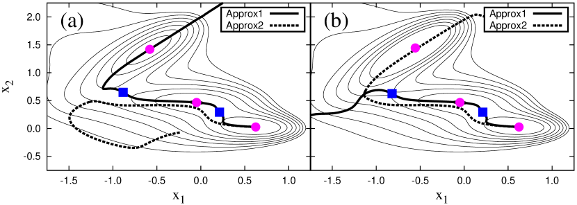
Figure 2: The potential energy surfaces made by the Müller-Brown potential [20], i.e., (a) the modified one $V_{\mathrm{MB}}^{(a)}$ and (b) the original one $V_{\mathrm{MB}}^{(b)}$, together with the collective paths extracted by the Approx1 and Approx2 methods. The circles denote the local minima and the squares the saddle points. The solid (dashed) line represents the collective path calculated by the Approx1 (Approx2) method, which starts from one of the local minima. The thin lines denote the contours of the potential energy surfaces.

In Fig. 2, we summarize four collective paths that are extracted from the Hamiltonians with $V_{\mathrm{MB}}^{(a)}$ and $V_{\mathrm{MB}}^{(b)}$ by the Approx1 and Approx2 methods. In Refs. [17, 18], the Approx1 method was thought to be a better method than the Approx2 method. For $V_{\mathrm{MB}}^{(a)}$, indeed, the Approx1 method can produce the collective path between local minima, while the Approx2 method is not the case. For $V_{\mathrm{MB}}^{(b)}$, however, the approximation that extracts the transition event is not the Approx1 method but the Approx2 method. Figure 3 depicts all paths based on the Approx1 method. We note that, in contrast to $V_{\mathrm{MB}}^{(a)}$, $V_{\mathrm{MB}}^{(b)}$ has no single path connecting the local minima. It turns out that whether the Approx1 method or the Approx2 method can extract the transition event sensitively depends on the shape of the potential energy surface, and hence both the Approx1 and Approx2 methods have not been a robust construction method of the collective path.

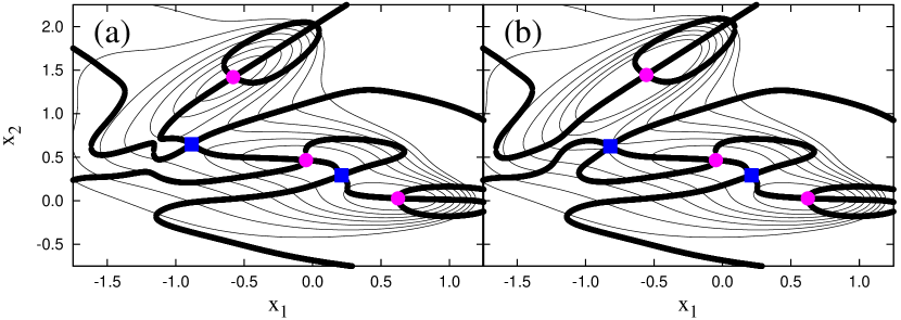
Figure 3: All the paths derived by the Approx1 method for (a) $V_{\mathrm{MB}}^{(a)}$ and (b) $V_{\mathrm{MB}}^{(b)}$.

3 Improvement of approximations to decoupling conditions in self-consistent theory of large-amplitude collective motion

In this section, we develop the numerical simulation method that can robustly construct the collective path connecting local minima, which is an improvement of the Approx1 and Approx2 methods. A key point for the development of the method is the construction of $Y={}^{t}(X_{i},\,\Phi_{a},\,\Lambda,\,\Gamma)$ as an optimal solution to Eq. (11).

By constructing the optimal solution $Y$ and substituting $Y$ into Eq. (9), we can obtain a first-order differential equation to determine $(x_{i},\,\varphi_{i},\,\lambda,\,\gamma)$ as a solution to an initial-value problem.

We shall construct a procedure to obtain the optimal solution to Eq. (11). To this end, first we define a vector $\Delta$, which represents a deviation from the equality in Eq. (11), that is,

$$\Delta\equiv A\,Y-b.$$ (30)

Here, we treat the problem to minimize the magnitude of $\Delta$ to derive an equation for the construction of the optimal $Y$.

3.1 Measure of deviation from exact decoupling

We introduce three new vectors $d_{i}$, $e_{i}$, and $f_{i}$ to represent $\Delta$ as a form of the modification into $\varphi_{i}$ in the elements of $A$ and $b$. Indeed, by parameterizing $\Delta$ as

$$\Delta={\scriptstyle\left(\begin{array}[]{c}G_{ij}\,(d_{j}-\varphi_{j})\\ \Gamma\,(e_{i}-\varphi_{i})\\ f_{i}-\varphi_{i}\end{array}\right)},$$ (34)

with

$$G_{ij}\equiv\Lambda\,\delta_{ij}-V_{,ijk}\,X_{k},$$ (35)

we can convert Eq. (30) into the same form as Eq. (11):

$$\tilde{A}\,Y-\tilde{b}=0,$$ (36)

where

$$\tilde{A} \equiv {\scriptstyle\left(\begin{array}[]{cccc}V_{,ijk}\,d_{k}&(V_{,ij}-\lambda\,\delta_{ij})\,\varphi_{\perp j}^{a}&-d_{i}&0\\ V_{,ij}&-\gamma\,\varphi_{\perp i}^{a}&0&-e_{i}\\ \delta_{ij}&0&0&0\end{array}\right)},$$ (40)

$$\tilde{b} \equiv {}^{t}(0,\,0,\,f_{i}).$$ (41)

Here, $\tilde{A}$ and $\tilde{b}$ are obtained by the replacement of $\varphi_{i}$ in the first and second rows of $A$ and the third row of $b$ to $d_{i}$, $e_{i}$, and $f_{i}$, respectively. Because the condition $d_{i}=e_{i}=f_{i}=\varphi_{i}$ reproduces the exact decoupling conditions, we can reach the following natural definition of the scalar quantity that measures the deviation from exact decoupling:

$$Q=\sum_{i=1}^{N}\,\Big{(}w_{d}\,(d_{i}-\varphi_{i})^{2}+w_{e}\,(e_{i}-\varphi_{i})^{2}+w_{f}\,(f_{i}-\varphi_{i})^{2}\Big{)},$$ (42)

where $w_{d}$, $w_{e}$, and $w_{f}$ denote weight parameters to determine which decoupling conditions (3)-(5) are respected. Because we are interested in the case where all of the decoupling conditions (3)-(5) are respected equivalently, we must set

$$(w_{d},\,w_{e},\,w_{f})=(1,\,1,\,1).$$ (43)

By definition, the set of $(w_{d},\,w_{e},\,w_{f})=(1,\,1,\,0)$ corresponds to the Approx1 method, while the set of $(w_{d},\,w_{e},\,w_{f})=(1,\,0,\,1)$ leads to the Approx2 method.

To make clear a geometrical meaning of $Q$, we rewrite $Q$ as

$$Q={}^{t}\Delta\,C\,\Delta={}^{t}(A\,Y-b)\,C\,(A\,Y-b).$$ (44)

This representation means that $Q$ is identical to the norm, i.e., the square of the length of the vector $\Delta=A\,Y-b$ measured on the metric $C$ given by

$$C\equiv{\scriptstyle\left(\begin{array}[]{ccc}[{}^{t}(G^{-1})\,G^{-1}]_{ij}&0&0\\ 0&\Gamma^{-2}\,\delta_{ij}&0\\ 0&0&\delta_{ij}\end{array}\right)}.$$ (48)

It is obvious that $C$ has a dependence on $(X_{i},\,\Lambda,\,\Gamma)$ that is not yet determined.

As shown in Eqs. (18)-(21), $Y={}^{t}(X_{i},\,\Phi_{a},\,\Lambda,\,\Gamma)$ can be obtained without reference to $C$ at the local minima and saddle points $x_{i}^{\mathrm{eq}}$. If we take $x_{i}^{\mathrm{eq}}$ as a starting point to detect the collective path, we can carry out a straightforward construction of $C$ by substituting $(X_{i},\,\Lambda,\,\Gamma)$ in Eqs. (18), (20), and (21) into Eq. (48). Here, we refer to $C$ constructed at the starting point $x_{i}^{\mathrm{eq}}$ as $C^{\mathrm{eq}}$.

In this work, we use this metric $C^{\mathrm{eq}}$ as a substitute for $C$ in the course of the detection of the collective path;

$$C=C^{\mathrm{eq}}.$$ (49)

Thanks to the metric $C$ being constant, $Q$ is a function bilinear with respect to $Y$, which is easily minimized. It is left to future work to carry out the nonlinear optimization of $Q$ with respect to $Y$ by taking into account the $Y$-dependence in $C$.

3.2 Basic equation of proper construction method of collective path

By applying the minimization (stationary) condition $\partial Q/\partial Y=0$ to $Q$ with $C=C^{\mathrm{eq}}$, we arrive at

$$({}^{t}A\,C^{\mathrm{eq}}\,A)\,Y-{}^{t}A\,C^{\mathrm{eq}}\,b=0.$$ (50)

We note that in contrast to Eq. (11), Eq. (50) can have a definite solution in general because ${}^{t}A\,C^{\mathrm{eq}}\,A$ is a $(2\,N+1)\times(2\,N+1)$ matrix and the number of the equations agrees with that of the variables. We stress that Eq. (9) combined with $Y$ that is a solution to Eq. (50) is the main equation for the construction of the collective path, which is one of the results in this work.

A few remarks are in order here: (i) The basic equation of our method given by the set of Eqs. (9) and (50) is a first-order differential equation with respect to $(x_{i},\,\varphi_{i},\,\lambda,\,\gamma)$, which can be solved with a single iteration for the stepwise construction of the collective path by repeating the calculation of the elements of the matrix $A$. In fact, we can construct $A$ without an iteration procedure, because the elements of $A$ are given by only the first, second, and third derivatives of the potential energy with respect to the coordinate variables, which can be calculated at a given structure of the system. Furthermore, we note that the elements associated with the third derivatives of $V(\mbox{\boldmath$x$})$ in the matrix $A$ in Eq. (50) can be calculated in the same computational cost as that in the case of the second derivative terms because the third derivative terms enter into $A$ as a form of $V_{,ijk}\,\varphi_{k}$. Indeed, we can construct $V_{,ijk}\,\varphi_{k}$ from the two second derivatives on the basis of the formula

$$V_{,ijk}(\mbox{\boldmath$x$})\,\varphi_{k}\sim\frac{V_{,ij}(\mbox{\boldmath$x$}+\mbox{\boldmath$n$}\,\Delta x)-V_{,ij}(\mbox{\boldmath$x$}-\mbox{\boldmath$n$}\,\Delta x)}{2\,\Delta x},$$ (51)

with $\mbox{\boldmath$n$}\equiv(\varphi_{1}/\sqrt{m_{1}},\,\cdots,\,\varphi_{N}/\sqrt{m_{N}})$. Here, $\Delta x$ denotes an infinitesimal value. We note that the calculations of the two second derivatives can be run in parallel. Thanks to Eq. (51), the resultant method requires only the numerical calculation of the first and second derivatives in each step of the single iteration. This property reduces the computational costs considerably. (ii) As mentioned in the final paragraph in Sec. 2.2, we suppose that the initial value of $(x_{i},\,\varphi_{i},\,\lambda,\,\gamma)$ is set equal to $(x^{\mathrm{eq}}_{i},\,\phi^{0}_{i},\,\lambda^{0},\,0)$. Here, we present an account of the eigenvalue $\lambda^{0}$ and eigenvector $\phi^{0}_{i}$. In this work, we adopt the smallest eigenvalue as $\lambda^{0}$. This is because we are interested in the rare transition event of molecular systems where the amplitude of the collective coordinate is large compared to those of the other coordinates, which can be translated to the requirement to use the smallest eigenvalues of $V_{,ij}$. We note that the direction of the construction of the collective path from the initial configuration depends on the sign of $\phi^{0}_{i}$, because $\phi^{0}_{i}$ gives the step from the initial structure to the next one.

4 Applications of self-consistent theory of large-amplitude collective motion to simple Hamiltonians

In this section, first we examine our method’s ability to construct the collective path connecting local minima. Then, we elucidate the ability of the method to extract the rare transition event by using potential energy surfaces with either a high energy barrier or a narrow gate to separate the two local minima as shown in Fig. 1.

4.1 Müller-Brown potential

To examine the robustness property of the numerical simulation method based on the set of Eqs. (9) and (50), we utilize the Hamiltonians with the Müller-Brown potential [20], which are the same as those presented in Fig. 2.

Figure 4: The collective paths constructed by the method based on the set of Eqs. (9) and (50). The potential energy surfaces are the same as those in Fig. 2, and the solid line represents the collective path.

In Fig. 4, we show the resultant collective paths. Both of them are shown as trajectories that connect almost all the local minima and saddle points. As that it is not the case in the collective paths obtained with the Approx1 and Approx2 methods, shown in Fig. 2, we conclude that our method is a robust construction method of the collective path describing the transition between local minima, in contrast to the Approx1 and Approx2 methods.

We now make one remark here. The collective paths depicted in Fig. 4 pass close to but not exactly through the saddle points. This is a critical problem for the studies of minimum energy path [21, 22]. However, the path studied in this paper is the one including not only the potential energy but also the kinetic energy. In this case, that the path passes exactly through the saddle points is not necessarily required. A further examination of this point is a future problem.

4.2 Barrier and gate potential

We consider a Hamiltonian given by

$$H=\frac{1}{2}\,(p_{1}^{2}+p_{2}^{2})+V_{\mathrm{BG}}(x_{1},\,x_{2}).$$ (52)

Here, $V_{\mathrm{BG}}(x_{1},\,x_{2})$ denotes the barrier and gate potential defined by

$$V_{\mathrm{BG}}(x_{1},\,x_{2})=-\frac{1}{2}\,a\,x^{2}_{1}+\frac{1}{4}\,b\,x^{4}_{1}+(x_{2}-c\,x_{1})^{2}\,\Big{[}\alpha\,x^{2}_{1}+\beta\,\mathrm{e}^{-\gamma\,x^{2}_{1}}+\delta\Big{]},$$ (53)

with $(a,\,b,\,c,\,\alpha,\,\beta,\,\gamma,\,\delta)$ being parameters. The parameters $(a,\,b,\,c)$ determine locations and energy values of stationary points. Indeed, this potential energy surface has two local minima and one saddle point located at $(\pm\sqrt{a/b},\,\pm c\,\sqrt{a/b})$ and $(0,\,0)$, respectively, and the activation energy in the transition between the two local minima is given by $a^{2}/(4\,b)$. The parameters $(\alpha,\,\beta,\,\gamma,\,\delta)$ determine the narrowness of the pathway connecting the local minima and the saddle point.

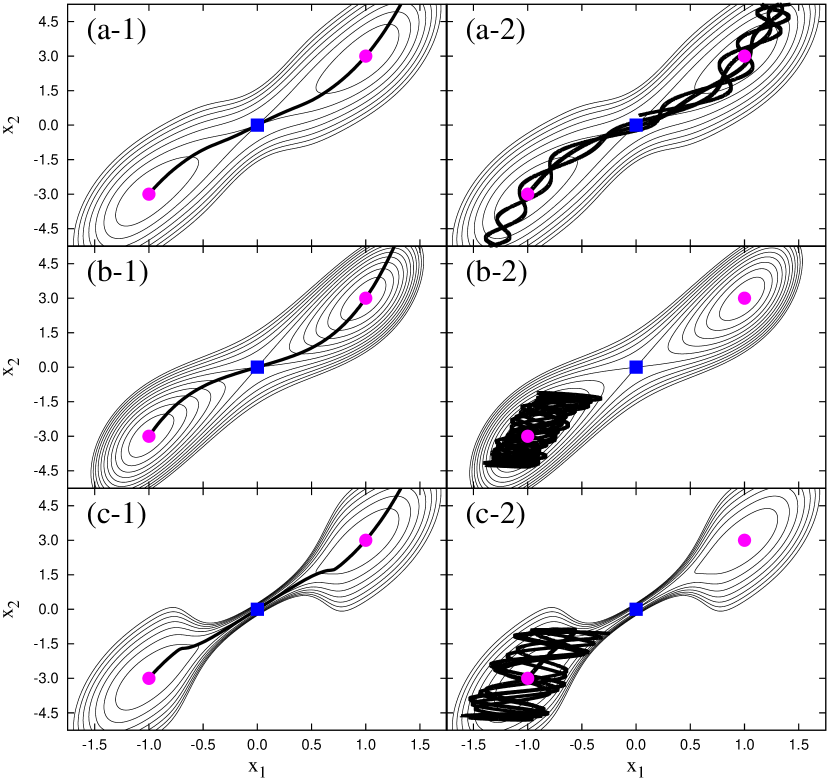
Figure 5: The collective paths obtained by the method developed in this work and the trajectories obtained by the MD method on the $V_{\mathrm{BG}}^{(a)}$, $V_{\mathrm{BG}}^{(b)}$, and $V_{\mathrm{BG}}^{(c)}$ potential energy surfaces. The solid lines in (a-1) and (a-2) ((b-1) and (b-2) or (c-1) and (c-2)) show the collective path and the MD trajectory derived from $V_{\mathrm{BG}}^{(a)}$ ($V_{\mathrm{BG}}^{(b)}$ or $V_{\mathrm{BG}}^{(c)}$), respectively. In (a-1) and (a-2) ((b-1) and (b-2) or (c-1) and (c-2)), the thin lines denote the contours of $V_{\mathrm{BG}}^{(a)}$ ($V_{\mathrm{BG}}^{(b)}$ or $V_{\mathrm{BG}}^{(c)}$), the circles the local minima, and the squares the saddle point.

To show the ability of the method developed to simulate the rare transition event, we introduce three potential energy surfaces: a potential energy surface containing neither a high energy barrier nor a narrow gate $V_{\mathrm{BG}}^{(a)}$, a surface with a high energy barrier $V_{\mathrm{BG}}^{(b)}$, and a surface with a narrow gate $V_{\mathrm{BG}}^{(c)}$. The parameters $(a,\,b,\,c,\,\alpha,\,\beta,\,\gamma,\,\delta)$ which create $V_{\mathrm{BG}}^{(a)}$, $V_{\mathrm{BG}}^{(b)}$, and $V_{\mathrm{BG}}^{(c)}$ read $(80,\,80,\,3,\,0.0045,\,10,\,10,\,1)$, $(240,\,240,\,3,\,0,\,0,\,10,\,20)$, and $(80,\,80,\,3,\,0.31,\,690,\,10,\,9.7)$, respectively. All the potential energies have the same locations of the local minima as $(\pm 1,\,\pm 3)$.

In Fig. 5, we show the collective paths corresponding to $V_{\mathrm{BG}}^{(a)}$, $V_{\mathrm{BG}}^{(b)}$, and $V_{\mathrm{BG}}^{(c)}$ together with trajectories obtained by the conventional MD method. We find that the collective paths provide pathways connecting the two local minima even if a high energy barrier or narrow gate exists between the two local minima. Conversely, the MD method applied to $V_{\mathrm{BG}}^{(a)}$ can provide a trajectory near the collective path, but the trajectories obtained for the $V_{\mathrm{BG}}^{(b)}$ and $V_{\mathrm{BG}}^{(c)}$ cases are seen to be trapped near one local minimum and cannot reach the other local minimum. We note that the qualitatively same results are obtained with less symmetric potentials, e.g., $V_{\mathrm{BG}}(x_{1},\,x_{2})+x_{1}^{3}$; in B, the results for the potentials are discussed. We stress that in contrast to the MD method, our method works well as a simulation technique for the rare transition event.

5 Summary and concluding remarks

Basic notion adopted in this work is that simulation of rare transition events can reduce to construction of a collective path given as a simple sharp curve along which only one coordinate increases if the initial coordinates are adequately chosen. To detect the collective path, we have developed a method to separate a collective coordinate, which parametrizes the collective path, from the other coordinates orthogonal to the collective coordinate. The method has been formulated by constructing the collective path as an optimal solution to the decoupling conditions in the self-consistent theory of large-amplitude collective motion proposed by Dang et al. [15, 16, 17, 18]. A basic equation of the method is given by the set of Eqs. (9) and (50). We have found that the equation is a first-order differential equation that determines the collective path as a solution to an initial-value problem from an arbitrary point in the collective path with the use of the first and second derivatives of the potential energy with respect to the atomic coordinates. By using the Müller-Brown potential [20], we have demonstrated that the method, which is an improvement of the theory of Dang et al., can robustly construct the collective path connecting the local minima in the potential energy surface. We have used a simple potential energy surface to show that our method uses only the initial configuration to construct a pathway to the final configuration, even if the configurations are separated by a high energy barrier and/or a narrow gate.

We consider that our study can stimulate discussions about the rare transition events in various systems of interest. In fact, the method presented in this work can be applied to simulate the rare transition events of generic molecular systems whose potential energy surfaces are well-defined. For example, by using a potential energy for biomolecules, e.g., the generalized amber force field [23], we will demonstrate [24] that our method can be applied to describe allosteric transitions [2, 3] which are typical rare transition events for protein systems. Furthermore, if we utilize potential energies calculated numerically using computer programs developed on the basis of quantum chemistry, we can describe a chemical reaction as a rare transition event. In fact, we will show [25] that combining this method with the density functional theory [26] allows simulation of an intermolecular proton transfer reaction, i.e., molecular dynamics with quantum tunneling. We will also show [27] that our method in combination with time-dependent density functional theory [28] can be applied to simulate photochemical reactions, i.e., the dynamics of molecular systems in electronic excited states.

Finally, we remark again the following study that should be reported in the near future. We apply the non-linear optimization to Eq. (44) to determine the collective path in a full consistent manner and compare it with the collective path obtained in the approximation (49).

Appendix A Detailed derivation of decoupling conditions

In this section, we present a review of the derivation of the decoupling conditions in the self-consistent theory of large-amplitude collective motion developed by Dang et al. [15, 16, 17, 18]. We focus on the collective path parametrized by one collective coordinate, although Dang et al. [15, 16, 17, 18] have presented a construction method of a multi-dimensional collective path, i.e., the so-called collective surface. Basically, we obey the notation used in Refs. [17, 18] in this section. In the final stage, we convert the derived decoupling conditions into those introduced in Sec. 2.1.

We treat an $N$-body system whose Hamiltonian is

$$H=\frac{1}{2}\,\pi_{\alpha}\,B^{\alpha\beta}\,\pi_{\beta}+V(\xi^{1},\,\cdots,\,\xi^{N}).$$ (54)

Here, $\alpha$ and $\beta$ denote indices that vary from $1$ to $N$, $\xi^{\alpha}$ and $\pi_{\alpha}$ are a coordinate and its conjugate momentum of the $\alpha$-th degree of freedom, respectively, $B^{\alpha\beta}$ is a reciprocal mass tensor, and $V(\xi^{1},\,\cdots,\,\xi^{N})$ is a potential energy. We suppose that $B^{\alpha\beta}$ is diagonalized as

$$B^{\alpha\beta}=\mathrm{diag}(1/m_{1},\,\cdots,\,1/m_{N}),$$ (55)

with $m_{\alpha}$ being the mass of the $\alpha$-th degree of freedom.

We use a canonical transformation to obtain conditions that define the collective path. In the canonical transformation, we consider mappings of the form

$$\xi^{\alpha}=g^{\alpha}(q^{1},\,\cdots,\,q^{N})\equiv g^{\alpha}(q),$$ (56)

whose inverse relations are given by

$$q^{\mu}=f^{\mu}(\xi^{1},\,\cdots,\,\xi^{N})\equiv f^{\mu}(\xi).$$ (57)

Using a chain rule relation, we find that $g^{\alpha}(q)$ and $f^{\mu}(\xi)$ satisfy the following relations:

$$\delta^{\alpha}_{\,\,\,\beta} = \partial\xi^{\alpha}/\partial\xi^{\beta}=g^{\alpha}_{,\,\mu}(q)\,f^{\mu}_{,\,\beta}(\xi),$$ (58)

$$\delta^{\mu}_{\,\,\,\nu} = \partial q^{\mu}/\partial q^{\nu}=f^{\mu}_{,\,\alpha}(\xi)\,g^{\alpha}_{,\,\nu}(q),$$ (59)

where the comma indicates a partial derivative; $F_{,\,\alpha}(\xi)\equiv\partial F(\xi)/\partial\xi^{\alpha}$ and $G_{,\,\mu}(q)\equiv\partial G(q)/\partial q^{\mu}$. The indices $\alpha,\,\beta,\,\cdots$ represent those of the initial coordinates, and $\mu,\,\nu,\,\cdots$ those of the final coordinates, although each set has the same range $1,\,\cdots,\,N$. The momentum $p_{\mu}$ conjugate to $q^{\mu}$ is given by

$$p_{\mu}=g^{\alpha}_{,\,\mu}(q)\,\pi_{\alpha},$$ (60)

with inverse

$$\pi_{\alpha}=f^{\mu}_{,\,\alpha}(\xi)\,p_{\mu}.$$ (61)

The Hamiltonian as described with the canonical coordinates $(q^{\mu},\,p_{\mu})$ is

$$H=\frac{1}{2}\,p_{\mu}\,\bar{B}^{\mu\nu}(q)\,p_{\nu}+\bar{V}(q).$$ (62)

Here, $\bar{B}^{\mu\nu}(q)$ is an inverse matrix of $\bar{B}^{-1}_{\mu\nu}(q)$ given by

$$\bar{B}^{-1}_{\mu\nu}(q)\equiv g^{\alpha}_{,\,\mu}(q)\,B^{-1}_{\alpha\beta}\,g^{\beta}_{,\,\nu}(q),$$ (63)

and $\bar{V}(q)$ is the potential energy written by $q^{\mu}$ as

$$\bar{V}(q)\equiv V(\xi^{1}=g^{1}(q),\,\cdots,\,\xi^{N}=g^{N}(q)).$$ (64)

Equations of motion derived from the Hamiltonian (62) are

$$\dot{q}^{\mu} = \bar{B}^{\mu\nu}(q)\,p_{\nu},$$ (65)

$$\dot{p}_{\mu} = -\frac{1}{2}\,p_{\nu}\,\bar{B}^{\nu\rho}_{,\,\mu}(q)\,p_{\rho}-\bar{V}_{,\,\mu}(q).$$ (66)

In the new canonical coordinates, we identify the collective path as follows: We divide the set of $(q^{\mu},\,p_{\mu})$ into two subsets, $(q^{1},\,p_{1})$ and $(q^{a},\,p_{a})$ with $a=2,\,\cdots,\,N$, and suppose this division to ensure that if at time $t=0$ both $q^{a}=0$ and $p_{a}=0$, then $q^{a}(t)=0$ and $p_{a}(t)=0$. The time evolution of $q^{1}$ and $p_{1}$ in the new canonical coordinates can be converted into that of $\xi^{\alpha}$ and $\pi_{\alpha}$ which takes place on a two-dimensional subspace

$$\xi^{\alpha} = \hat{\xi}^{\alpha}\equiv g^{\alpha}(\hat{q}),$$ (67)

$$\pi_{\alpha} = \hat{\pi}_{\alpha}\equiv f^{\mu}_{,\,\alpha}(\hat{\xi})\,\hat{p}_{\mu},$$ (68)

with

$$\hat{q}^{\mu} \equiv (q^{1},\,0,\,\cdots,\,0),$$ (69)

$$\hat{p}_{\mu} \equiv (p_{1},\,0,\,\cdots,\,0).$$ (70)

We note that $q^{1}$ is the collective coordinate and $\hat{\xi}^{\alpha}$ is identical to the collective path parametrized by $q^{1}$.

The requirements $(\dot{q}^{a},\,\dot{p}_{a})=(0,\,0)$ can be compatible with the requirements $(q^{a},\,p_{a})=(0,\,0)$ only if the equations

$$0 = \bar{B}^{a1}(\hat{q})\,p_{1},$$ (71)

$$0 = -\frac{1}{2}\,p_{1}\,\bar{B}^{11}_{,\,a}(\hat{q})\,p_{1}-\bar{V}_{,\,a}(\hat{q}),$$ (72)

are satisfied, as one sees from Eqs. (65) and (66). Equations (71) and (72) are equivalent to three conditions

$$\bar{B}^{a1}(\hat{q}) = 0,$$ (73)

$$\bar{V}_{,\,a}(\hat{q}) = 0,$$ (74)

$$\bar{B}^{11}_{,\,a}(\hat{q}) = 0.$$ (75)

Here, we have assumed that $p^{1}$ is not a constant of the motion. We emphasize that these equations determine an explicit form of $\hat{\xi}^{\alpha}$. In fact, if $g^{\alpha}_{,\,1}(\hat{q})$ is obtained as a solution to Eqs. (73)-(75), we can construct $\hat{\xi}^{\alpha}=\hat{\xi}^{\alpha}(q^{1})$ by solving a differential equation

$$\frac{\mathrm{d}}{\mathrm{d}q^{1}}\hat{\xi}^{\alpha}=g^{\alpha}_{,\,1}(\hat{q}),$$ (76)

which has been derived from the definition (67).

From here on, we convert Eqs. (73)-(75) into convenient forms to obtain an explicit form of $g^{\alpha}_{,\,1}(\hat{q})$. For this purpose, first we introduce two scalar quantities

$$X^{(0)}(\xi) \equiv V(\xi)$$ (77)

$$= \bar{V}(q)\equiv\bar{X}^{(0)}(q),$$

$$X^{(1)}(\xi) \equiv V_{,\,\alpha}(\xi)\,B^{\alpha\beta}\,V_{,\,\beta}(\xi)$$ (78)

$$= \bar{V}_{,\,\mu}(q)\,\bar{B}^{\mu\nu}(q)\,\bar{V}_{,\,\nu}(q)\equiv\bar{X}^{(1)}(q).$$

These quantities have an important property given by

$$\bar{X}^{(\sigma)}_{,\,a}(\hat{q})=0,\,\,\,\sigma=0,\,1.$$ (79)

Here, we present a proof for the above equations. The proof for the case of $\sigma=0$ is trivial as follows:

$$\bar{X}^{(0)}_{,\,a}(\hat{q})=\bar{V}_{,\,a}(\hat{q})=0,$$ (80)

which is just Eq. (74). In the case of $\sigma=1$, we simply compute

$$\bar{X}^{(1)}_{,\,a}(\hat{q}) = 2\,\bar{X}^{(0)}_{,\,\mu a}(\hat{q})\,\bar{X}^{(0)}_{,\,\nu}(\hat{q})\,\bar{B}^{\mu\nu}(\hat{q})+\bar{X}^{(0)}_{,\,\mu}(\hat{q})\,\bar{X}^{(0)}_{,\,\nu}(\hat{q})\,\bar{B}^{\mu\nu}_{,\,a}(\hat{q})$$ (81)

$$= 2\,\bar{X}^{(0)}_{,\,ba}(\hat{q})\,\bar{X}^{(0)}_{,\,1}(\hat{q})\,\bar{B}^{b1}(\hat{q})+2\,\bar{X}^{(0)}_{,\,1a}(\hat{q})\,\bar{X}^{(0)}_{,\,1}(\hat{q})\,\bar{B}^{11}(\hat{q})$$

$${}+\bar{X}^{(0)}_{,\,1}(\hat{q})\,\bar{X}^{(0)}_{,\,1}(\hat{q})\,\bar{B}^{11}_{,\,a}(\hat{q})$$

$$= 0.$$

In passing to the second equality, we have used $\bar{X}^{(0)}_{,\,a}(\hat{q})=0$ proved in Eq. (80). We have then used Eqs. (73) and (75) in the first and third terms, respectively, to make these vanish, whereas the second term vanishes because $\bar{X}^{(0)}_{,\,1a}(\hat{q})=0$ which can be derived from $\bar{X}^{(0)}_{,\,a}(\hat{q})=0$.

Then, we rewrite Eq. (79) as

$$B^{\alpha\beta}\,X^{(\sigma)}_{,\,\beta}(\hat{\xi})=\bar{X}^{(\sigma)}_{,\,1}(\hat{q})\,g^{\alpha}_{,\,1}(\hat{q})\,\bar{B}^{11}(\hat{q}),\,\,\,\sigma=0,\,1.$$ (82)

Here, we have used relations

$$X^{(\sigma)}_{,\,\alpha}(\hat{\xi})=\bar{X}^{(\sigma)}_{,\,\mu}(\hat{q})\,f^{\mu}_{,\,\alpha}(\hat{\xi})=\bar{X}^{(\sigma)}_{,\,1}(\hat{q})\,f^{1}_{,\,\alpha}(\hat{\xi}),$$ (83)

$$B^{\alpha\beta}\,f^{1}_{,\,\beta}(\hat{\xi})=g^{\alpha}_{,\,\mu}(\hat{q})\,\bar{B}^{\mu 1}(\hat{q})=g^{\alpha}_{,\,1}(\hat{q})\,\bar{B}^{11}(\hat{q}),$$ (84)

which have been derived from the chain rule and Eqs. (58), (59), (63), and (77)-(79). We note that Eq. (82) is an alternative form of Eqs. (73)-(75) because Eq. (82) can be derived only if all of Eqs. (73)-(75) are used.

Substituting the explicit forms

$$X^{(0)}_{,\,\alpha}(\hat{\xi}) = V_{,\,\alpha}(\hat{\xi}),$$ (85)

$$X^{(1)}_{,\,\alpha}(\hat{\xi}) = 2\,V_{,\,\alpha\beta}(\hat{\xi})\,B^{\beta\gamma}\,V_{,\,\gamma}(\hat{\xi}),$$ (86)

into Eq. (82), we have

$$B^{\alpha\beta}\,V_{,\,\beta}(\hat{\xi})=\gamma(\hat{q})\,g^{\alpha}_{,\,1}(\hat{q}),$$ (87)

$$\Big{[}B^{\alpha\gamma}\,V_{,\,\gamma\beta}(\hat{\xi})\,-\lambda(\hat{q})\delta^{\alpha}_{\,\,\,\beta}\Big{]}\,g^{\beta}_{,\,1}(\hat{q})=0,$$ (88)

with

$$\gamma(\hat{q}) \equiv \bar{X}^{(0)}_{,\,1}(\hat{q})\,\bar{B}^{11}(\hat{q}),$$ (89)

$$\lambda(\hat{q}) \equiv \frac{\bar{X}^{(1)}_{,\,1}(\hat{q})}{2\,\bar{X}^{(0)}_{,\,1}(\hat{q})}.$$ (90)

Owing to a scale indefiniteness in the definition of $q^{1}$, there exists an ambiguity for the overall amplitude of $g^{\alpha}_{,\,1}(\hat{q})$. Without loss of generality, we can adopt the normalization

$$g^{\alpha}_{,\,1}(\hat{q})\,B^{-1}_{\alpha\beta}\,g^{\beta}_{,\,1}(\hat{q})=1.$$ (91)

We note that Eqs. (76), (87), (88), and (91) are identical to the decoupling conditions. By setting

$$\xi^{\alpha=i} = x_{i},$$ (92)

$$g^{\alpha=i}_{,\,1}(\hat{q}) = \varphi_{i}/\sqrt{m_{i}},$$ (93)

$$q^{1} = q,$$ (94)

we find that Eqs. (76), (87), (88), and (91) correspond to Eqs. (3), (5), (4), and (6), respectively.

Appendix B Barrier and gate potential with less symmetry

A Hamiltonian we consider is given by

$$H=\frac{1}{2}\,(p_{1}^{2}+p_{2}^{2})+V^{\prime}_{\mathrm{BG}}(x_{1},\,x_{2}).$$ (95)

Here, $V^{\prime}_{\mathrm{BG}}(x_{1},\,x_{2})$ denotes the barrier and gate potential with less symmetry defined by

$$V^{\prime}_{\mathrm{BG}}(x_{1},\,x_{2})=V_{\mathrm{BG}}(x_{1},\,x_{2})-\frac{1}{3}\,\epsilon\,x^{3}_{1},$$ (96)

where $V_{\mathrm{BG}}(x_{1},\,x_{2})$ has been given in Eq. (53). We note that the term associated with $\epsilon$ breaks the symmetry with respect to $x_{1}\rightarrow-x_{1}$. This potential energy surface has two local minima and one saddle point located at $(\epsilon/2b\pm\sqrt{\epsilon^{2}/4b^{2}+a/b},\,c\epsilon/2\,b\pm c\sqrt{\epsilon^{2}/4b^{2}+a/b})\equiv(x_{1\pm}^{\mathrm{eq}},\,x_{2\pm}^{\mathrm{eq}})$ and $(0,\,0)$, respectively, and the activation energies in the transitions from $(x_{1+}^{\mathrm{eq}},\,x_{2+}^{\mathrm{eq}})$ to $(x_{1-}^{\mathrm{eq}},\,x_{2-}^{\mathrm{eq}})$ and from $(x_{1-}^{\mathrm{eq}},\,x_{2-}^{\mathrm{eq}})$ to $(x_{1+}^{\mathrm{eq}},\,x_{2+}^{\mathrm{eq}})$ are given by $a^{2}/4b+a\epsilon^{2}/4b^{2}+\epsilon^{4}/24b^{3}\pm(a\epsilon/3b+\epsilon^{3}/12b^{2})\sqrt{\epsilon^{2}/4b^{2}+a/b}$, respectively.

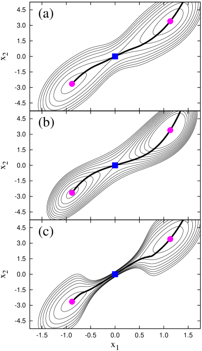
Figure 6: The collective paths obtained by the method developed in this work on the $V_{\mathrm{BG}}^{\prime(a)}$, $V_{\mathrm{BG}}^{\prime(b)}$, and $V_{\mathrm{BG}}^{\prime(c)}$ potential energy surfaces. The solid lines in (a) ((b) or (c)) show the collective path derived from $V_{\mathrm{BG}}^{\prime(a)}$ ($V_{\mathrm{BG}}^{\prime(b)}$ or $V_{\mathrm{BG}}^{\prime(c)}$), respectively. In (a) ((b) or (c)), the thin lines denote the contours of $V_{\mathrm{BG}}^{\prime(a)}$ ($V_{\mathrm{BG}}^{\prime(b)}$ or $V_{\mathrm{BG}}^{\prime(c)}$), the circles the local minima, and the squares the saddle point.

We introduce three potential energy surfaces: a potential energy surface containing neither a high energy barrier nor a narrow gate $V_{\mathrm{BG}}^{\prime(a)}$, a surface with a high energy barrier $V_{\mathrm{BG}}^{\prime(b)}$, and a surface with a narrow gate $V_{\mathrm{BG}}^{\prime(c)}$. The parameters $(a,\,b,\,c,\,\alpha,\,\beta,\,\gamma,\,\delta,\,\epsilon)$ which create $V_{\mathrm{BG}}^{\prime(a)}$, $V_{\mathrm{BG}}^{\prime(b)}$, and $V_{\mathrm{BG}}^{\prime(c)}$ read $(80,\,80,\,3,\,0.0045,\,10,\,10,\,1,\,20)$, $(240,\,240,\,3,\,0,\,0,\,10,\,20,\,60)$, and $(80,\,80,\,\break 3,\,0.31,\,690,\,10,\,9.7,\,20)$, respectively. All the potential energies have the same locations of the local minima as $((1\pm\sqrt{65})/8,\,3(1\pm\sqrt{65})/8)$.

In Fig. 6, we show the collective paths for $V_{\mathrm{BG}}^{\prime(a)}$, $V_{\mathrm{BG}}^{\prime(b)}$, and $V_{\mathrm{BG}}^{\prime(c)}$. It reveals that the collective paths provide pathways connecting the two local minima. We stress that these results are qualitatively the same as those of the symmetric potentials $V^{(a)}_{\mathrm{BG}}$, $V^{(b)}_{\mathrm{BG}}$, and $V^{(c)}_{\mathrm{BG}}$ examined in Sec. 4.2.

References

- [1] P. G. Debrunner and H. Frauenfelder, Ann. Rev. Phys. Chem. 33 (1982), 283.
- [2] Chou KC, Biophys. Chem. 20 (1984), 61.
- [3] O. Miyashita, J. N. Onuchic, and P. G. Wolynes, Proc. Natl. Acad. Sci. USA, 100 (2003), 12570.
- [4] J. A. McCammon, Rep. Prog. Phys. 47 (1984), 1.
- [5] N. Nakajima, J. Phys. Chem. B 101 (1997), 817.
- [6] Y. Sugita and Y. Okamoto, Chemical Phys. Lett. 314 (1999), 141.
- [7] A. Laio and M. Parrinello, Proc. Natl. Acad. Sci. USA 99 (2002), 12562.
- [8] Y. Fukunishi, Y. Mikami, and H. Nakamura, J. Phys. Chem. B 107 (2003), 13201.
- [9] S. Tomonaga, Prog. Theor. Phys. 13 (1955), 467.
- [10] S. Tomonaga, Prog. Theor. Phys. 13 (1955), 482.
- [11] T. Marumori, T. Maskawa, F. Sakata, and A. Kuriyama, Prog. Theor. Phys. 64 (1980), 1294.
- [12] M. Matsuo and K. Matsuyanagi, Prog. Theor. Phys. 74 (1985), 288.
- [13] M. Matsuo, Prog. Theor. Phys. 76 (1986), 372.
- [14] M. Matsuo, T. Nakatsukasa and K. Matsuyanagi, Prog. Theor. Phys. 103 (2000), 959.
- [15] G. Do Dang, A. Bulgac, and A. Klein, Phys. Rev. C 36 (1987), 2661.
- [16] N. R. Walet, A. Klein, and G. Do Dang, J. Chem. Phys. 91 (1989), 2848.
- [17] A. Klein, N. R. Walet, and G. Do Dang, Ann. Phys. 208 (1991), 90.
- [18] G. D. Dang, A. Klein and N. R. Walet, Phys. Rep. 335 (2000), 93.
- [19] H. Aoyama and H. Kikuchi, Nucl. Phys. B 369 (1992), 219.
- [20] K. Müller and L. D. Brown, Theor. Chim. Acta. 53 (1979), 75.
- [21] K. Fukui, S. Kato, and H. Fujimoto, J. Am. Chem. Soc. 97 (1975), 1.
- [22] G. Henkelman and H. Jónsson, J. Chem. Phys. 113 (2000), 9978.
- [23] J. Wang, R. M. Wolf, J. W. Caldwell, P. A. Kollman, and D. A. Case, J. Comput. Chem. 25 (2004), 1157.
- [24] K. Tsumura et al., in preparation.
- [25] K. Tsumura et al., in preparation.
- [26] W. Kohn and L. J. Sham, Phys. Rev. 140 (1965), A1133.
- [27] K. Tsumura et al., in preparation.
- [28] E. Runge and E. K. U. Gross, Phys. Rev. Lett. 52 (1984), 997.