Primordial Magnetic Helicity Constraints from WMAP Nine-Year Data

Abstract

If a primordial magnetic field in the universe has non-zero helicity, the violation of parity symmetry results in non-zero correlations between cosmic microwave background temperature and B-mode polarization. In this paper we derive approximations to the relevant microwave background power spectra arising from a helical magnetic field. Using the cross-power spectrum between temperature and B-mode polarization from the WMAP nine-year data, we set a 95% confidence level upper limit on the helicity amplitude to be 10 nG² Gpc for helicity spectral index $n_{H}=-1.9$, for a cosmological magnetic field with effective field strength of 3 nG and a power-law index $n_{B}=-2.9$ near the scale-invariant value. Future microwave background polarization maps with greater sensitivity will be able to detect the helicity of an inflationary magnetic field well below the maximum value allowed by microwave background constraints on the magnetic field amplitude.

I Introduction

A challenging question of modern astrophysics is the origin of observed magnetic fields in galaxies and clusters Widrow . Generally, fields observed today began as small seed fields and then were amplified via either adiabatic compression or through turbulent plasma dynamics. One mechanism for seed field generation is generic plasma instabilities and vorticity perturbations Kulsrud:2007an . In this causal model, the correlation length of the resulting fields is limited by the horizon, which generically corresponds to comoving galaxy scales. A second possibility is larger seed fields generated during inflation spanning a wide range of correlation lengths up to the horizon today, and amplified through the process of cosmological structure growth Kandus:2010nw ; Durrer:2013pga .

The evolution and amplification of a primordial seed field is strongly influenced by the helicity, or local handedness, of the seed field. Magnetic helicity is a manifestation of parity symmetry violation. While the level of parity violation observed in fundamental physical interactions is small, parity violation is widespread in various astrophysical systems with significant magnetic dynamics, such as one-sided jets from active galactic nuclei and helical magnetic fields in the solar magnetosphere Brandenburg:2004jv . A seed field with helicity is restructured at large scales by plasma turbulence: the decay of the magnetic field leads to an increase in the relative magnetic helicity until the helicity saturates at the maximum value allowed by the realizability condition for the field strength. The magnetic field correlation length of a helical magnetic field will also increase more quickly than for a non-helical field due to the inverse cascade mechanism. Magnetic fields with maximal helicity are a generic outcome of any extended period of turbulence tevzadze .

Helical magnetic fields can be generated during the electroweak phase transition or during inflation Cornwall:1997ms ; Giovannini:1997eg ; Field:1998hi ; Vachaspati:2001nb ; Tashiro:2012mf ; Sigl:2002kt ; Subramanian:2004uf ; Campanelli:2005ye ; semikoz05 ; DiazGil:2007dy ; Campanelli:2008kh ; Campanelli:2013mea . Such a helical cosmological magnetic field might be the source of magnetic helicity needed in galactic dynamo amplification models Banerjee:2004 . Thus testing the helicity of any primordial magnetic field is important for understanding the origin of observed astrophysical magnetic fields Widrow . Magnetic helicity in strong local magnetic fields like astrophysical jets can be deduced from the polarization of synchrotron radiation deduction1 ; deduction2 . For cosmological magnetic helicity the detection issue is more difficult, because the field strengths are much lower and the observational effects more subtle.

The most direct probe of any cosmological magnetic fields is their effect on the cosmic microwave background radiation, and particularly its polarization. The microwave background linear polarization is conventionally decomposed into E-mode (parity-even) and B-mode (parity-odd) components kks97 ; sz97 . A non-helical magnetic field contributes to all of the parity-even power spectra, those correlating E with itself and B with itself, in addition to E with the microwave temperature T and the temperature with itself. These contributions were explicitly calculated in Ref. mack02 , and have been used to constrain the amplitude of a primordial magnetic field Shaw:2009nf ; Yamazaki:2011eu ; Yamazaki:2010jw ; Yamazaki:2010nf ; Paoletti:2012bb ; Paoletti:2010rx ; Kunze:2010ys ; Ade:2013zuv . However, if a parity-violating helical magnetic field component is present, then it will contribute to the remaining parity-odd power spectra, namely EB or TB pogosian02 ; cdk04 ; kr05 ; Kunze:2011bp , which are identically zero for magnetic fields with zero helicity. Note that Faraday rotation by magnetic fields kl96 imprints itself on the power spectrum and frequency spectrum of microwave background polarization, but is insensitive to helicity for a given magnetic field power spectrum Ensslin:2003ez ; Campanelli:2004pm ; Kosowsky:2004zh ; kmk08 .

Helical magnetic fields are perhaps the most natural parity-violating source of TB or EB correlations in the microwave background polarization Cabella:2007br ; Xia:2007qs ; Feng:2006dp ; Xia:2012ck ; Xia:2009ah ; Li:2009rt ; Li:2008tma ; Gruppuso:2011ci , but other more speculative parity-violating sources can also induce them. These include a Chern-Simons coupling of photons to another field Lue:1998mq ; Feng:2006dp ; Cabella:2007br ; Xia:2007qs ; Xia:2008si ; Saito:2007kt , a homogeneous magnetic field Scannapieco:1997mt ; Scoccola:2004ke ; Demianski:2007fz ; Kristiansen:2008tx , Lorentz symmetry breaking Carroll:1989vb ; Kostelecky:2007zz ; Cai:2009uc ; Ni:2007ar ; Casana:2008ry ; Caldwell:2011pu ; MosqueraCuesta:2011tz ; Kamionkowski:2010rb ; Gluscevic:2010vv ; Mewes:2012sm ; Gluscevic:2012me ; Ni:2009qm ; Miller:2009pt ; Ni:2009gz , or non-trivial cosmological topology Lim:2004js ; Carroll:2004ai ; Alexander:2006mt ; Satoh:2007gn . If some non-zero TB or EB correlation is detected, the corresponding angular power spectrum must be measured sufficiently well to distinguish between these possibilities.

In this paper we obtain upper limits on the helicity of a primordial magnetic field, using the nine-year WMAP constraints on any cross correlation between microwave background temperature and B-polarization komatsu . Current polarization data is consistent with zero cosmological TB signal, as expected in the standard cosmological model. We compute the theoretical estimates of cross correlation given in Ref. kr05 and compare with the measured upper limits komatsu ; Hinshaw:2013 ; Larson:2010gs . Since we obtain only upper limits, we assume that magnetic helicity is the only possible parity-violating source present, which gives the most conservative helicity upper limits. For simplicity of calculation, we consider only the vector (vorticity) perturbations sourced by the magnetic field and neglect the tensor (gravitational wave) perturbations. This is a good approximation for angular multipoles $l>50$ cdk04 , and for this reason we use measured $C_{l}^{TB}$ constraints only for $l>50$; the neglected large angular scales contain little total statistical weight in our constraints.

The outline of the paper is as follows: in Sec. II we review the main characteristics of a helical magnetic field and derive the vorticity perturbations. Section III gives the expression for $C_{l}^{TB}$ due to these vorticity perturbations, and these are compared with the WMAP 9-year upper limits in Sec. IV. Implications and future experimental prospects are discussed in Sec. V. We employ natural units with $\hbar=c=1$ and gaussian units for electromagnetic quantities.

II Properties of a Cosmological Magnetic Field

We assume that a cosmological magnetic field was generated during or prior to the radiation-dominated epoch, with the energy density of the field being a first-order perturbation to the standard Friedmann-Lemaître-Robertson-Walker homogeneous cosmological model. We also assume that primordial plasma is a perfect conductor and thus the spatial and temporal dependence of the field separates: ${\mathbf{B}}({\mathbf{x}},t)={\mathbf{B}}({\mathbf{x}})/a(t)^{2}$ with $a(t)$ the cosmological scale factor. The mean helicity density of the magnetic field is given by

$${\mathcal{H}}_{B}=\frac{1}{V}\int_{V}d{\bf x}{\bf A({\bf x})}\cdot{\bf B({\bf x})}=\frac{1}{V}\int_{V}d{\bf x}{\bf A({\bf x})}\cdot\nabla\times{\bf A({\bf x})},$$ (1)

with $\bf A$ the vector potential, in the limit that the integral is over an infinite volume. An integral over a finite but large volume will approximate this helicity density. In general, magnetic helicity is a gauge-dependent quantity, because the vector potential ${\bf A}$ can be redefined by adding a gradient to it. However, the magnetic helicity is gauge invariant for periodic systems without a net magnetic flux, as shown in Ref. gauge . We assume that our universe can be well approximated by a large box with periodic boundary conditions, provided the dimension of the box is large compared to the Hubble length today. In this case, the magnetic helicity is a well-defined quantity.

A Gaussian random magnetic field is described by the two-point correlation function in wavenumber space as

$$\langle B^{*}_{m}({\mathbf{k}})B_{n}({\mathbf{k}^{\prime}})\rangle=(2\pi)^{3}\delta^{(3)}({\mathbf{k}}-{\mathbf{k}^{\prime}})\left[(\delta_{mn}-\hat{k}_{m}\hat{k}_{n})P_{B}(k)+i\epsilon_{mnl}\hat{k}_{l}P_{H}(k)\right].$$ (2)

Here $\hat{k}_{m}=k_{m}/k$ are the unit wavenumber components, $\epsilon_{mnl}$ is the antisymmetric tensor, and $\delta^{(3)}({\mathbf{k}}-{\mathbf{k}^{\prime}})$ is the Dirac delta function. We use the Fourier transform convention $B_{j}({\mathbf{k}})=\int d^{3}x\,e^{i{\mathbf{k}}\cdot{\mathbf{x}}}B_{j}({\mathbf{x}})$. The symmetric power spectrum $P_{B}(k)$ is related to the mean magnetic energy density by

$${\mathcal{E}}_{B}=\frac{1}{(2\pi)^{3}}\int_{0}^{k_{D}}dkk^{2}P_{B}(k),$$ (3)

while the antisymmetric power spectrum $P_{H}(k)$ is related to the magnetic helicity density as

$${\mathcal{H}}_{B}=\frac{1}{(2\pi)^{3}}\int_{0}^{k_{D}}dkk\frac{1}{2}P_{H}(k),$$ (4)

where $k_{D}$ is a characteristic damping scale for the magnetic field.

The total energy density and helicity of the magnetic field satisfy the realizability condition

$${\mathcal{H}}_{B}\leq 2\xi_{M}{\mathcal{E}}_{B},$$ (5)

where

$$\xi_{M}\equiv\frac{2\pi\int_{0}^{k_{D}}dkkP_{B}(k)}{\int_{0}^{k_{D}}dkk^{2}P_{B}(k)}$$ (6)

is the magnetic field correlation length. The power spectra $P_{B}(k)$ and $P_{H}(k)$ are generically constrained by $P_{B}(k)\geq|P_{H}(k)|$. We assume that these power spectra are given by simple power laws, $P_{B}(k)=A_{B}k^{n_{B}}$ and $P_{H}(k)=A_{H}k^{n_{H}}$. The constraint on their relative amplitudes implies $n_{H}>n_{B}$ durrer03 ; in addition, finiteness of the total magnetic field energy requires $n_{B}>-3$ if the power law extends to arbitrarily small values of $k$. For physical transparency, instead of describing the magnetic field amplitude by the proportionality factors $A_{B}$ and $A_{H}$, we will use the effective magnetic field amplitude $B_{\rm eff}\equiv(8\pi{\mathcal{E}}_{B})^{1/2}$ ktr11 and the helicity density ${\mathcal{H}}_{B}$. Using these quantities is convenient because they do not depend on the power law indices $n_{B}$ and $n_{H}$ and are independent of any smoothing scale.

Often, cosmological magnetic fields are characterized by a smoothed value on some comoving length scale $\lambda>\lambda_{D}=2\pi/k_{D}$. Convolving with a Gaussian smoothing kernel, the smoothed magnetic field amplitude $B_{\lambda}$ is mack02

$${B_{\lambda}}^{2}\equiv|\langle{\mathbf{B}}({\mathbf{x}})\cdot{\mathbf{B}}({\mathbf{x}})\rangle|_{\lambda}=\frac{2}{(2\pi)^{2}}A_{B}\Gamma\left(\frac{n_{B}+3}{2}\right)\lambda^{-n_{B}-3},\qquad\qquad\lambda>\lambda_{D}.$$ (7)

We also introduce a smoothed quantity $H_{\lambda}$ (the so-called helicity measure or current helicity Kunze:2011bp ) related to the magnetic helicity having the same units as $B_{\lambda}$ and depending on the antisymmetric part of the magnetic field spectrum:

$$H_{\lambda}^{2}\equiv\lambda|\langle{\mathbf{B}}({\mathbf{x}})\cdot[{\mathbf{\nabla}}\times{\mathbf{B}}({\mathbf{x}})]\rangle|_{\lambda}=\frac{2}{(2\pi)^{2}}A_{H}\Gamma\left(\frac{n_{H}+4}{2}\right)\lambda^{-n_{H}-3},\qquad\qquad\lambda>\lambda_{D}.$$ (8)

See Ref. Kosowsky:2004zh for a more detailed discussion. Then the transformation between the smoothed quantities $B_{\lambda}$ and $H_{\lambda}$ and the effective quantities ${B}_{\rm eff}$ and ${\mathcal{H}}_{B}$ is simply

$$B_{\rm eff}=\frac{B_{\lambda}(k_{D}\lambda)^{\frac{n_{B}+3}{2}}}{\sqrt{\Gamma\left(\frac{n_{B}+5}{2}\right)}}\;,$$ (9)

and

$${\mathcal{H}}_{B}=\frac{1}{8\pi}\frac{\lambda H_{\lambda}^{2}(k_{D}\lambda)^{n_{H}+2}}{(n_{H}+2)\Gamma\left(\frac{n_{H}+4}{2}\right)}\;.$$ (10)

We assume that the magnetic field cutoff scale $k_{D}$ is determined by the Alfvén wave damping scale, $\lambda_{D}\simeq v_{A}L_{S}$ sub98b ; jedamzik98 , where $v_{A}$ is the Alfvén velocity set by the total magnetic energy density mack02 . Since $v_{A}\ll 1$ the Alfvén damping scale will always be much smaller scale than the Silk damping scale (the thickness of the last scattering surface) for standard cosmological models. On the other hand, the CMB fluctuations are determined by the Silk damping scale, and presence of the magnetic field source at smaller scales will not significantly affect the resulting spectra.

III Microwave Background Fluctuations from a Helical Magnetic Field

A cosmological magnetic field induces Alfvén waves sourced by the Lorentz force in the cosmological plasma (see dky98 ; mack02 ; jedamzik98 ; sub98b ; Seshadri:2000ky ; Subramanian:2003sh ), which generically produce non-zero vorticity perturbations. In the case of a stochastic magnetic field the average Lorentz force $\langle{\bf L(x)}\rangle=-\langle{\bf B}\times[{\bf\nabla}\times{\bf B}]\rangle/(4\pi)$ vanishes, while the root-mean-square Lorentz force $\langle{\bf L(x)\cdot L(x)}\rangle^{1/2}$ is non-zero and acts as a source in the vector perturbation equation. If the magnetic field spectrum Eq. (2) has a helical part $P_{H}(k)$, then the Lorentz force two-point correlation function will have both symmetric and antisymmetric pieces. Both contribute to the symmetric piece of the vorticity perturbation spectrum, but only the antisymmetric piece of the Lorentz force, determined entirely by $P_{H}(k)$, will contribute to the antisymmetric part of the vorticity perturbation spectrum kr05 .

In the tight-coupling limit between photons and baryons, the fluid vorticity is sourced by the transverse and divergence-free piece of the Lorentz force. The fluid vorticity at last scattering then translates into temperature and polarization fluctuations in the microwave background radiation mack02 . The microwave temperature and E-polarization components are both parity-symmetric, while the B-polarization component is parity-antisymmetric hu97 . This implies that the cross-power spectra $C_{l}^{TB}$ and $C_{l}^{EB}$ from stochastic magnetic fields will be nonzero only if $P_{H}(k)$ is nonzero kks97 ; pogosian02 ; cdk04 ; kr05 ; Kunze:2011bp . In other words, the $TB$ and $EB$ power spectra provide a way to measure whether a primordial magnetic field has a helical component. (A constant magnetic field component also gives non-zero $C_{l}^{TB}$ and $C_{l}^{EB}$ through Faraday rotation Scannapieco:1997mt ; Scoccola:2004ke , but the two distinct contributions can be distinguished by their different power spectra, and by the frequency dependence of a Faraday rotation signal.)

Detailed computations of the various CMB angular power spectra induced by helical and nonhelical magnetic fields have been presented elsewhere kr05 ; mack02 . Here we focus on the TB power spectrum, because current data does not put a significant constraint on the much smaller EB power spectrum. For $l>50$ where the TB power spectrum has significant power, we neglect tensor contributions, which are smaller. Here we derive an analytic approximation to the TB angular power spectrum, based on the second-order approximation technique from Ref. Zaldarriaga:1995gi ; this approximate solution is simple and accurate enough for deriving upper limits on the helical magnetic field.

The multipoles of the temperature perturbation from a vector mode in Fourier space are given by

$$\frac{\Theta^{(\pm 1)}_{l}(k,\eta_{0})}{2l+1}\simeq\sqrt{\frac{l(l+1)}{2}}~{}\Omega^{(\pm 1)}(k,\eta_{\rm dec})\frac{j_{l}(k\eta_{0})}{k\eta_{0}},\qquad l\geq 2$$ (11)

where $\Omega^{\pm 1}(k,\eta)$ are the two helicity components of the gauge-invariant vorticity perturbations, constructed from the fluid velocity field and the vector component of the metric perturbations kr05 . Here we have made the approximation $\eta_{0}-\eta_{\rm dec}\simeq\eta_{0}$ in Eq. (11). For vorticity perturbations sourced by the magnetic field, the $l=1$ moment of temperature fluctuation is well approximated by the vorticity perturbation, $\Theta^{(\pm 1)}(k,\eta_{0})\simeq\Omega^{\pm 1}(k,\eta_{\rm dec})$ mack02 . For the B-mode polarization perturbation, we have mack02

$$\frac{B^{(\pm 1)}_{l}(k,\eta_{0})}{2l+1}\simeq\mp\frac{\sqrt{6}}{2}\sqrt{(l-1)(l+2)}\int^{\eta_{0}}_{0}d\eta{\dot{\tau}}(\eta)e^{-\tau}P^{(\pm 1)}(k,\eta)\frac{j_{l}(k\eta_{0}-k\eta)}{k\eta_{0}-k\eta}\;,$$ (12)

where the polarization source is defined by hu97

$$P^{(\pm 1)}=\frac{1}{10}\bigl{[}\Theta^{(\pm 1)}_{2}-\sqrt{6}E^{(\pm 1)}_{2}\bigr{]}.$$ (13)

The temperature and polarization quadrupoles satisfy the evolution equations

$$\dot{\Theta}^{(\pm 1)}_{2} = k\bigl{[}\frac{\sqrt{3}}{3}\Theta^{(\pm 1)}_{1}-\frac{2\sqrt{2}}{7}\Theta^{(\pm 1)}_{3}\bigr{]}+{\dot{\tau}}\left[\Theta^{(\pm 1)}_{2}-P^{(\pm 1)}\right]\;,$$ (14)

$$\dot{E}^{(\pm 1)}_{2} = k\bigl{[}\mp\frac{1}{3}B^{(\pm 1)}_{2}-\frac{2\sqrt{10}}{21}E^{(\pm 1)}_{3}\bigr{]}+{\dot{\tau}}\left[E^{(\pm 1)}_{2}+\sqrt{6}P^{(\pm 1)}\right]\;.$$ (15)

Here the optical depth $\tau(\eta)=\int_{\eta}^{\eta_{0}}d\eta^{\prime}{\dot{\tau}}(\eta^{\prime})$ to photon scattering from conformal time $\eta$ until today satisfies $d\tau/d\eta\equiv-{\dot{\tau}}(\eta)=\sigma_{T}n_{e}(\eta)a(\eta)$, $\sigma_{T}$ is the Thomson scattering cross section, and $n_{e}(\eta)$ the comoving number density of free electrons. The vector mode of the CMB temperature-$B$ polarization angular power spectrum is given by hu97

$$C^{TB~{}(V)}_{l}=\frac{2}{\pi}\int dkk^{2}\left[\frac{\Theta^{(-1)*}_{l}(k,\eta_{0})}{2l+1}\frac{B^{(-1)}_{l}(k,\eta_{0})}{2l+1}+\frac{\Theta^{(+1)*}_{l}(k,\eta_{0})}{2l+1}\frac{B^{(+1)}_{l}(k,\eta_{0})}{2l+1}\right]\;.$$ (16)

In the rest of this section, we approximate this power spectrum in a given cosmological model, for comparison with limits on this power spectrum from temperature and polarization sky maps.

The visibility function ${\dot{\tau}}e^{-\tau}$ is sharply peaked at the time of decoupling, so to determine the $B$-polarization signal, Eq. (12), we need to know the polarization source $P^{(\pm 1)}$ at the time of decoupling. Differentiating Eq. (13) with respect to conformal time and substituting Eqs. (14) and (15), at leading order we get

$$\dot{P}^{(\pm 1)}-\frac{3}{10}{\dot{\tau}}P^{(\pm 1)}\simeq\frac{k\sqrt{3}}{30}\Theta^{(\pm 1)}_{1}\;,$$ (17)

where we have dropped terms containing $\Theta^{(\pm 1)}_{3},E^{(\pm 1)}_{3}$ and $B^{(\pm 1)}_{2}$ (see also Ref. Zaldarriaga:1995gi ).

In our previous work kr05 ; mack02 , we assumed the first term of Eq. (17) is small to obtain the approximate solution $P^{(\pm 1)}=\sqrt{3}k\Theta_{1}^{(\pm 1)}/9{\dot{\tau}}$. While usually valid, this approximation fails during recombination because $k/\dot{\tau}$ varies rapidly: inserting $P^{(\pm 1)}=\sqrt{3}k\Theta_{1}^{(\pm 1)}/9{\dot{\tau}}$ into the integral of Eq. (12), the integrand becomes proportional to $e^{-\tau}$, and is not anymore peaked at the time of decoupling. Instead, we employ a more precise second-order approximate solution to the source equation, following the technique in Refs. Zaldarriaga:1995gi ; Cai:2012ci . Details are given in the Appendix; the solution for the temperature-B polarization power spectrum is,

$$C_{l}^{TB} \simeq -\frac{3\pi}{14}\ln\left(\frac{10}{3}\right)\sqrt{\frac{(l+2)!}{(l-2)!}}\frac{(n_{B}+3)(n_{H}+2)}{n_{B}+n_{H}+2}\frac{\eta_{\rm dec}^{2}}{\eta_{0}^{2}}{k_{D}\Delta\eta_{\rm dec}}\frac{1}{(1+R_{\rm dec})^{2}}$$ (18)

$$\times\frac{{\cal E}_{B}{\cal H}_{B}k_{D}}{\rho_{\gamma\,0}^{2}}\int_{0}^{x_{S}}dx\,x^{4}D_{E}(x)\left[1+\frac{n_{H}-1}{n_{B}+3}x^{n_{B}+n_{H}+2}\right]j_{l}^{2}(xk_{D}\eta_{0})$$

with the change of variables $x=k/k_{D}$ in the integral. We have defined a function which models the effect of Silk damping for polarization Cai:2012ci ,

$$D_{E}(x)\equiv 0.2\left(e^{-c_{E}(a_{1}xk_{D}\eta_{0})^{b_{E}}}+e^{-c_{E}(a_{2}xk_{D}\eta_{0})^{b_{E}}}\right)$$ (19)

with the fitting constants $c_{E}=0.27$, $b_{E}=2.0$, $a_{1}=0.0011$, and $a_{2}=0.0019$. The amplitude of the approximate solution Eq. (18) differs from that in Ref. mack02 by roughly a factor of two.

IV Constraints from WMAP

We obtain constraints on primordial magnetic helicity by comparing the temperature-$B$-polarization cross correlation function in Eq. (18) with WMAP nine-year data. We assume a standard $\Lambda$CDM model. We take the Silk damping scale to be the thickness of the last scattering surface, $L_{S}\simeq\Delta\eta_{\rm dec}$, which is determined by the function $D_{E}(x)$, so $k_{S}=0.3$ Mpc^-1. The WMAP $C_{l}^{TB}$ measurement is consistent with a null signal, as expected in the standard cosmological model. We follow a Feldman-Cousins prescription Feldman:1997qc to set $68\%$ and $95\%$ confidence level (CL) upper limits on the primordial magnetic field komatsu . We only consider multipoles with $\ell>50$ to simplify the analysis; in this range the measured values of $C_{\ell}^{TB}$ are uncorrelated between different $\ell$ values. This restriction does not significantly impact sensitivity to the magnetic field, since most signal is for larger values of multipole number.

A comparison between our model for $C_{\ell}^{TB}$ and the nine-year WMAP data is given in Fig. 1 for two magnetic field helicity models: one with power law $n_{H}=-1.9$ and amplitude ${\mathcal{H}}_{B}=10^{5}$ nG² Mpc, and one with power law $n_{H}=-0.6$ and amplitude ${\mathcal{H}}_{B}=10^{8}$ nG² Mpc. For both cases, we set the value of the effective magnetic field $B_{\rm eff}$ to 1 nG and the spectral index to its inflationary value of $n_{B}=-2.99$, which is somewhat below current cosmological limits current_limits . These models both produce a helical magnetic field which is just at the level which can be ruled out from the WMAP 9-year microwave background polarization power spectra. The helicity amplitude ${\mathcal{H}}_{B}$ varies strongly with spectral index, because for larger values of $n_{H}$ the helicity is more concentrated on small scales, close to the damping scale, which contribute little to the microwave background signal.

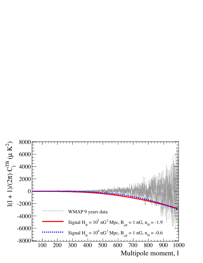
Figure 1: A comparison between the temperature-$B$-polarization cross correlation model for $B_{\rm eff}$ = 1 nG, $n_{B}=-2.99$; the solid red line is for a helicity amplitude of ${\mathcal{H}}_{B}=10^{5}$ nG² Mpc and helicity spectral index $n_{H}=-1.9$ while the dotted blue line is for ${\mathcal{H}}_{\rm B}=10^{8}$ nG² Mpc and $n_{H}$ = -0.6. Also shown are the nine-year WMAP data (solid gray dots with bars indicating uncertainties).

The upper limits on the ${\mathcal{H}}_{B}$ as functions of $n_{H}$ are given in Fig. 2 for three scenarios: $n_{B}=-2.99$, $n_{B}=-2.0$, and $n_{B}=n_{H}-1$.

Figure 2: The 95% upper limits on ${\mathcal{H}}_{B}$ as a function of $n_{H}$ for $n_{B}=-2.99$ (black solid), $n_{B}=-2.0$ (red short dash), and $n_{B}=n_{H}-1$ (blue long dash). For all three cases, $B_{\rm eff}=1$ nG.

We also present the limits in terms of $H_{\lambda}$ for the same three scenarios in Fig. 3, using a smoothing scale of $\lambda=1$ Mpc which is commonly used in the magnetic field literature.

Figure 3: The 95% upper limits on ${\mathcal{H}}_{\lambda}$ for a smoothing scale $\lambda=1$ Mpc, as a function of $n_{H}$ for $n_{B}=-2.99$ (black solid), $n_{B}=-2.0$ (red short dash), and $n_{B}=n_{H}-1$ (blue long dash). For all three cases, $B_{\rm eff}=1$ nG.

The results are relatively insensitive to the systematic uncertainty in the cross-correlation signal due to modeling of the cutoff scale; a plausible range of cutoff scales gives a signal difference which is smaller than the measurement uncertainties in the WMAP data. Systematic uncertainties with a size up to 20% of the predicted values of $C_{l}^{TB}$ have only small effects on the magnetic field limits obtained here.

V Conclusions

The results presented here are the first direct constraint on a helical primordial magnetic field by its contribution to the parity-odd temperature-B polarization cross-power spectrum $C_{l}^{TB}$ of the microwave background. No experiment to date has detected a non-zero value for this power spectrum; we use the WMAP 9-year measurement which is consistent with zero to place upper limits on the combined mean field strength and helicity of a primordial magnetic field. The primordial magnetic field amplitude constraint of around $B_{\rm eff}=3$ nG from the microwave background temperature and E-polarization power spectra Yamazaki:2013hda ; Shaw:2010ea ; Ade:2013zuv ; Kahniashvili:2012dy gives an upper limits on magnetic helicity ${\mathcal{H}}_{B}$ less than around 10 nG² Gpc for a nearly scale-invariant power spectrum with $n_{B}=-2.99$. The helicity limits become weaker for larger values of $n_{B}$. Recent work has argued for more stringent upper limits of $B_{\rm eff}<1$ nG from constraints on the trispectrum induced by magnetic fields, rather than the power spectrum trivedi14 . If magnetic fields from inflation are produced with a magnetic curvature mode as advocated by Ref. bonvin13 , then the trispectrum constraint is even stronger, pushing the magnetic field amplitude down to $B_{\rm eff}<0.05$ nG.

The mean helicity amplitude over a given volume is constrained by the realizability condition Eq. (5). The smaller the value of the magnetic field $B_{\rm eff}$, the lower the helicity ${\mathcal{H}}_{B}$ which can be supported by the field. Any cosmological field will have physical effects measured over an effective volume which is at most the Hubble volume, so the effective comoving correlation length of this field is limited by the Hubble length $H_{0}^{-1}$. For a given microwave background constraint on ${\mathcal{H}}_{B}$ and assuming a magnetic field strength equal to some current upper limit, the maximal magnetic helicity which saturates the realizability condition must have a correlation length $\xi_{M}=4\pi{\mathcal{H}}_{B}/B_{\rm eff}^{2}$. If this correlation length is larger than the Hubble length, then a magnetic field of the given amplitude cannot support helicity as large as the measured limit. For a magnetic field with $B_{\rm eff}=3$ nG and the corresponding helicity equal to the limiting value ${\mathcal{H}}_{B}=10$ nG² Gpc , the correlation length for maximal helicity is around 10 Gpc: current measurements provide a helicity constraint which is just at the level of the maximum possible helicity for the magnetic field strength. If the field strength is significantly lower, then the helicity limits derived in this paper are substantially above the maximum helicity allowed by Eq. (5).

Upcoming polarization data from the Planck satellite, as well as high-resolution ground-based experiments like ACTPol actpol and SPTPol sptpol , will strengthen limits on both the magnetic field amplitude and helicity, for two reasons: first, the signal increases for larger $l$ values beyond those probed by WMAP, and second, upcoming experiments will produce polarized maps over large portions of the sky with much greater sensitivity than WMAP. Interest in B-mode polarization has exploded due to the recent results from the BICEP2 collaboration bicep2 . Experiments searching for B-polarization from primordial tensor modes (at large angular scales) and gravitational lensing (at small angular scales) will drive continual increases in sensitivity over the coming decade. Planck’s maps have a sensitivity (around 85 $\mu$K-arcmin for the SMICA map) which is a factor of 4 lower than WMAP (around 360 $\mu$K-arcmin), corresponding to errors in $C_{l}^{TB}$ smaller by a factor of 16. The recent PRISM satellite proposal prism envisions full-sky polarization maps with sensitivity of 3 $\mu$K-arcmin, which would give $C_{l}^{TB}$ errors smaller than the WMAP errors used here by a factor of $10^{4}$.

Limits on the magnetic field amplitude $B_{\rm eff}$ from the microwave background power spectra will not improve substantially, because they are limited by cosmic variance in the power spectra from other non-magnetic sources of fluctuations. In contrast, sensitivity improvements in polarization will continue to improve helicity limits from $C_{l}^{TB}$ because this signal is not limited by cosmic variance: it is zero for standard-cosmology primary perturbations which do not violate parity. (At least this is the case until extreme sensitivities are reached where the cosmic variance in $C_{l}^{TB}$ from the residual gravitational lensing contribution to de-lensed maps dominates over the map noise). So future measurements may provide constraints on magnetic field helicity which are much below the maximal helicity allowed by Eq. (5) and the magnetic field amplitude limits.

The $TB$ power spectrum of cosmic microwave background polarization, and its lower-amplitude counterpart $EB$, provide a valuable opportunity to probe unconventional physics which violates cosmological parity. Of contributors to these power spectra, gravitational lensing and helical magnetic fields are the two sources which rely only on standard, demonstrated physical effects. The microwave background lensing spectrum can be calculated to high accuracy within the standard model of cosmological structure formation, so any departures from this signal would be a good bet for revealing the existence of significant helical magnetic fields in the universe. In turn, the detection of helicity would give valuable information about the still-mysterious origin of magnetic field in the cosmos.

Appendix A Derivation of $C^{TB~{}(V)}_{l}$

The solution of Eq. (17) can be written in the form

$$P^{(\pm 1)}=\frac{\sqrt{3}}{30}k\int^{\eta}_{0}d\eta^{\prime}e^{-\frac{3}{10}\tau(\eta,\eta^{\prime})}\Theta^{(\pm 1)}_{1}(\eta^{\prime})=\frac{\sqrt{3}}{30}k\int^{\eta}_{0}d\eta^{\prime}e^{+\frac{3}{10}\tau(\eta)}e^{-\frac{3}{10}\tau(\eta^{\prime})}\Theta^{(\pm 1)}_{1}(\eta^{\prime})\;,$$ (20)

where $\tau(\eta,\eta^{\prime})=\int^{\eta}_{\eta^{\prime}}d{\eta}^{\prime\prime}{\dot{\tau}}(\eta^{\prime\prime})=\tau(\eta^{\prime})-\tau(\eta)$ and the visibility function $V(\eta)=\frac{d}{d\eta}e^{-\tau(\eta)}={\dot{\tau}}e^{-\tau}$ can be approximated by the asymmetric Gaussian function gorbunov ; Cai:2012ci

$$V(\eta)=V(\eta_{\rm dec}){\rm exp}\bigl{[}-\frac{(\eta-\eta_{\rm dec})^{2}}{2\Delta\eta_{\rm dec}^{2}}\bigr{]}\;,$$ (21)

where $\Delta\eta_{\rm dec}=\Delta\eta_{{\rm dec}_{1}}\Theta(\eta_{\rm dec}-\eta)+\Delta\eta_{{\rm dec}_{2}}\Theta(\eta-\eta_{\rm dec})$, $\Delta\eta_{{\rm dec}_{1}}=0.0011\eta_{0}$ and $\Delta\eta_{{\rm dec}_{2}}=0.0019\eta_{0}$ and $\Theta(\eta)$ is the usual step function. The prefactor $V(\eta_{\rm dec})=\frac{1}{\sqrt{2\pi}\Delta\eta_{\rm dec}}$ is calculated from the normalization condition $\int^{\eta_{0}}_{0}V(\eta)d\eta=1$. Substituting the solution Eq. (20) into Eq. (12) we obtain

$$\frac{B^{\pm 1}_{l}(k,\eta_{0})}{2l+1}=\mp\frac{k}{10\sqrt{2}}\sqrt{(l-1)(l+2)}\int^{\eta_{0}}_{0}d\eta V(\eta)\frac{j_{l}(k(\eta_{0}-\eta))}{k(\eta_{0}-\eta)}\int^{\eta}_{0}d\eta^{\prime}e^{+\frac{3}{10}\tau(\eta)}e^{-\frac{3}{10}\tau(\eta^{\prime})}\Theta^{(\pm 1)}_{1}(\eta^{\prime})\;.$$ (22)

Since the visibility function $V(\eta)$ is sharply peaked around $\eta=\eta_{\rm dec}$ and $e^{-\frac{3}{10}\tau(\eta^{\prime})}$ behaves like a step function, the $\Theta^{(\pm 1)}_{1}(\eta^{\prime})$ factor can approximately be pulled out from the $\eta^{\prime}$ integration and we get

$$\frac{B^{\pm 1}_{l}(k,\eta_{0})}{2l+1}=\mp\frac{k}{10\sqrt{2}}\sqrt{(l-1)(l+2)}\int^{\eta_{0}}_{0}d\eta V(\eta)\frac{j_{l}(k(\eta_{0}-\eta))}{k(\eta_{0}-\eta)}\Theta^{(\pm 1)}_{1}(\eta)\int^{\eta}_{0}d\eta^{\prime}e^{+\frac{3}{10}\tau(\eta)}e^{-\frac{3}{10}\tau(\eta^{\prime})}\;.$$ (23)

Noticing that $V(\eta)\propto\exp(-\gamma(\eta-\eta_{\rm dec})^{2})$ and $j_{l}(k(\eta_{0}-\eta))$ contains a mixture of oscillating modes $e^{ip\eta}$ and $e^{-ip\eta}$ with $p\propto k$, the formula $\int_{-\infty}^{\infty}e^{-\gamma\eta^{2}}e^{ip\eta}d\eta=e^{-p^{2}/4\gamma}\int_{-\infty}^{\infty}e^{-\gamma\eta^{2}}d\eta$ gives the approximation Cai:2012ci

$$\int^{\eta_{0}}_{0}d\eta V(\eta)\frac{j_{l}(k(\eta_{0}-\eta))}{k(\eta_{0}-\eta)}\Theta^{(\pm 1)}_{1}(\eta)\approx\frac{j_{l}(k(\eta_{0}-\eta_{\rm dec})}{k\eta_{0}-k\eta_{\rm dec}}\Theta^{(\pm 1)}_{1}(\eta_{\rm dec})D_{E}(k)\int^{\eta_{0}}_{0}d\eta V(\eta)\;,$$ (24)

where $D_{E}(k)$ is the Silk damping factor for polarization Cai:2012ci , Eq. (19).

Introducing a new variable $x\equiv\tau(\eta^{\prime})/\tau(\eta)$, approximating $d\eta^{\prime}=-\Delta\eta_{\rm dec}dx/x$ and noticing that

$$\int^{\eta_{0}}_{0}d\eta~{}V(\eta)\int^{\infty}_{1}\frac{dx}{x}e^{-\frac{3}{10}x\tau(\eta)}e^{\frac{3}{10}\tau(\eta)}=\Delta\eta_{\rm dec}\cdot\int^{\infty}_{0}d\tau e^{-\frac{7}{10}\tau(\eta)}\int^{\infty}_{1}\frac{dx}{x}e^{-\frac{3}{10}x\tau(\eta)}=\Delta\eta_{\rm dec}\frac{10}{7}{\rm ln}\frac{10}{3}\;,$$ (25)

we get

$$\frac{B^{\pm 1}(k,\eta_{0})}{2l+1} = \mp\frac{\sqrt{2}}{14}{\rm ln}(\frac{10}{3})\sqrt{(l-1)(l+2)}D_{E}(k)\frac{j_{l}(k\eta_{0})}{k\eta_{0}}k\Delta\eta_{\rm dec}\Theta^{(\pm 1)}_{1}(k,\eta_{\rm dec})$$ (26)

$$= \mp\frac{\sqrt{2}}{14}{\rm ln}(\frac{10}{3})\sqrt{(l-1)(l+2)}D_{E}(k)k\Delta\eta_{\rm dec}\frac{j_{l}(k\eta_{0})}{k\eta_{0}}\Omega^{(\pm 1)}(k,\eta_{\rm dec})\;.$$ (27)

Making use of Eq. (27) and Eq. (11), we finally obtain for the temperature-$B$-polarization cross correlation function

$$C^{TB~{}(V)}_{l}=-\frac{2}{7\pi}{\rm ln}(\frac{10}{3})\sqrt{\frac{(l+2)!}{(l-2)!}}\int dkk^{2}D_{E}(k)\omega(k,\eta_{\rm dec})\frac{j_{l}^{2}(k\eta_{0})}{(k\eta_{0})^{2}}k\Delta\eta_{\rm dec}\;,$$ (28)

where $\omega(k)$ is the helical part of the power spectrum which can be expressed as kr05

$$\omega(k,\eta)=\left[\frac{k\eta}{(\rho_{\gamma,0}+p_{\gamma,0})(1+R_{\rm dec})}\right]^{2}g(k).$$ (29)

Here $p_{\gamma 0}$ and $\rho_{\gamma 0}$ are the radiation pressure and energy density today, $R_{\rm dec}$ is the baryon-photon energy density at decoupling, and $g(k)$ can be expressed in terms of the spectral indices $n_{B}$ and $n_{H}$, values of $B_{\lambda}$, $H_{\lambda}$, and the smoothing scale $\lambda$ as

$$g(k)={\mathcal{G}}\lambda k(\lambda k_{D})^{n_{B}+n_{H}+2}\left[1+\frac{n_{H}-1}{n_{B}+3}\left(\frac{k}{k_{D}}\right)^{n_{B}+n_{H}+2}\right]$$ (30)

with

$${\mathcal{G}}=\frac{\lambda^{3}B_{\lambda}^{2}H_{\lambda}^{2}}{24(n_{B}+n_{H}+2)\Gamma\left(\frac{n_{B}+3}{2}\right)\Gamma\left(\frac{n_{H}+4}{2}\right)}$$ (31)

Then using Eqs. (29), (30), and (31) in Eq. (28) we arrive at Eq. (18).

References

- (1) L. M. Widrow, “Origin of galactic and extragalactic magnetic fields,” Rev. Mod. Phys. 74, 775 (2002) [arXiv:astro-ph/0207240].
- (2) R. M. Kulsrud and E. G. Zweibel, “The Origin of Astrophysical Magnetic Fields,” Rept. Prog. Phys. 71, 0046091 (2008) [arXiv:0707.2783 [astro-ph]].
- (3) A. Kandus, K. E. Kunze and C. G. Tsagas, “Primordial magnetogenesis,” Phys. Rept. 505, 1 (2011). [arXiv:1007.3891 [astro-ph.CO]].
- (4) R. Durrer and A. Neronov, “Cosmological Magnetic Fields: Their Generation, Evolution and Observation,” Astron. Astrophys. Rev 21, 62 (2013). [arXiv:1303.7121 [astro-ph.CO]].
- (5) A. Brandenburg and K. Subramanian, “Astrophysical magnetic fields and nonlinear dynamo theory,” Phys. Rept. 417, 1 (2005) [arXiv:astro-ph/0405052].
- (6) A. G. Tevzadze, L. Kisslinger, A. Brandenburg and T. Kahniashvili, “Magnetic Fields from QCD Phase Transitions,” Astrophys. J. 759, 54 (2012) [arXiv:1207.0751 [astro-ph.CO]].
- (7) J. M. Cornwall, “Speculations on primordial magnetic helicity,” Phys. Rev. D 56, 6146 (1997) [arXiv:hep-th/9704022].
- (8) M. Giovannini and M. E. Shaposhnikov, “Primordial hypermagnetic fields and triangle anomaly,” Phys. Rev. D 57, 2186 (1998) [arXiv:hep-ph/9710234].
- (9) G. B. Field and S. M. Carroll, “Cosmological magnetic fields from primordial helicity,” Phys. Rev. D 62, 103008 (2000) [arXiv:astro-ph/9811206].
- (10) T. Vachaspati, “Estimate of the primordial magnetic field helicity,” Phys. Rev. Lett. 87, 251302 (2001) [arXiv:astro-ph/0101261].
- (11) H. Tashiro, T. Vachaspati and A. Vilenkin, “Chiral Effects and Cosmic Magnetic Fields,” Phys. Rev. D 86, 105033 (2012) [arXiv:1206.5549 [astro-ph.CO]].
- (12) G. Sigl, “Cosmological Magnetic Fields from Primordial Helical Seeds,” Phys. Rev. D 66, 123002 (2002) [arXiv:astro-ph/0202424].
- (13) K. Subramanian and A. Brandenburg, “Nonlinear current helicity fluxes in turbulent dynamos and alpha quenching,” Phys. Rev. Lett. 93, 205001 (2004) [arXiv:astro-ph/0408020].
- (14) L. Campanelli and M. Giannotti, “Magnetic helicity generation from the cosmic axion field,” Phys. Rev. D 72, 123001 (2005) [arXiv:astro-ph/0508653].
- (15) V. B. Semikoz and D. D. Sokoloff, “Magnetic helicity and cosmological magnetic field,” arXiv:astro-ph/0411496; “Large-scale cosmological magnetic fields and magnetic helicity,” Int. J. Mod. Phys. D 14, 1839 (2005).
- (16) A. Diaz-Gil, J. Garcia-Bellido, M. Garcia Perez and A. Gonzalez-Arroyo, “Magnetic field production during preheating at the electroweak scale,” Phys. Rev. Lett. 100, 241301 (2008) [arXiv:0712.4263 [hep-ph]].
- (17) L. Campanelli, “Helical Magnetic Fields from Inflation,” Int. J. Mod. Phys. D 18, 1395 (2009) [arXiv:0805.0575 [astro-ph]].
- (18) L. Campanelli, “Origin of Cosmic Magnetic Fields,” Phys. Rev. Lett. 111, no. 6, 061301 (2013) [arXiv:1304.6534 [astro-ph.CO]].
- (19) R. Banerjee and K. Jedamzik, “The evolution of cosmic magnetic fields: From the very early universe, to recombination, to the present,” Phys. Rev. D 70, 123003 (2004) [arXiv:astro-ph/0410032].
- (20) T. A. Ensslin, “Does circular polarisation reveal the rotation of quasar engines?,” Astron. Astrophys. 401, 499 (2003) [arXiv:astro-ph/0212387].
- (21) J.P. Vallée, New Astron. Rev. 48, 763 (2004).
- (22) M. Kamionkowski, A. Kosowsky, and A. Stebbins, “Statistics of Cosmic Microwave Background Polarization,” Phys. Rev. D 55, 7368 (1997) [arXiv:astro-ph/9611125].
- (23) M. Zaldarriaga and U. Seljak, “An all sky analysis of polarization in the microwave background,” Phys. Rev. D 55, 1830 (1997) [arXiv:astro-ph/9609170].
- (24) A. Mack, T. Kahniashvili and A. Kosowsky, “Vector and Tensor Microwave Background Signatures of a Primordial Stochastic Magnetic Field,” Phys. Rev. D 65, 123004 (2002) [arXiv:astro-ph/0105504].
- (25) J. R. Shaw and A. Lewis, “Massive Neutrinos and Magnetic Fields in the Early Universe,” Phys. Rev. D 81, 043517 (2010) [arXiv:0911.2714 [astro-ph.CO]].
- (26) D. G. Yamazaki, K. Ichiki, T. Kajino and G. J. Mathew, “Primordial Magnetic Field Effects on the CMB and Large Scale Structure,” Adv. Astron. 2010, 586590 (2010) [arXiv:1112.4922 [astro-ph.CO]].
- (27) D. G. Yamazaki, K. Ichiki, T. Kajino and G. .J. Mathews, “Constraints on the neutrino mass and the primordial magnetic field from the matter density fluctuation parameter ,” Phys. Rev. D 81, 103519 (2010) [arXiv:1005.1638 [astro-ph.CO]].
- (28) D. G. Yamazaki, K. Ichiki, T. Kajino and G. J. Mathews, “New Constraints on the Primordial Magnetic Field,” Phys. Rev. D 81, 023008 (2010) [arXiv:1001.2012 [astro-ph.CO]].
- (29) D. Paoletti and F. Finelli, “Constraints on a Stochastic Background of Primordial Magnetic Fields with WMAP and South Pole Telescope data,” Phys. Lett. B 726, 45 (2013) [arXiv:1208.2625 [astro-ph.CO]].
- (30) D. Paoletti and F. Finelli, “CMB Constraints on a Stochastic Background of Primordial Magnetic Fields,” Phys. Rev. D 83, 123533 (2011) [arXiv:1005.0148 [astro-ph.CO]].
- (31) K. E. Kunze, “CMB anisotropies in the presence of a stochastic magnetic field,” Phys. Rev. D 83, 023006 (2011) [arXiv:1007.3163 [astro-ph.CO]].
- (32) P. A. R. Ade et al. [Planck Collaboration], “Planck 2013 results. XVI. Cosmological parameters,” preprint (2013) [arXiv:1303.5076 [astro-ph.CO]].
- (33) L. Pogosian, T. Vachaspati and S. Winitzki, “Signatures of kinetic and magnetic helicity in the CMBR,” Phys. Rev. D 65, 083502 (2002) [arXiv:astro-ph/0112536].
- (34) C. Caprini, R. Durrer and T. Kahniashvili, “The cosmic microwave background and helical magnetic fields: The tensor mode,” Phys. Rev. D 69, 063006 (2004) [arXiv:astro-ph/0304556].
- (35) T. Kahniashvili and B. Ratra, “Effects of cosmological magnetic helicity on the cosmic microwave background,” Phys. Rev. D 71, 103006 (2005) [arXiv:astro-ph/0503709].
- (36) K. E. Kunze, “Effects of helical magnetic fields on the cosmic microwave background,” Phys. Rev. D 85, 083004 (2012) [arXiv:1112.4797 [astro-ph.CO]].
- (37) A. Kosowsky and A. Loeb, “Faraday rotation of microwave background polarization by a primordial magnetic field,” Astrophys. J. 469, 1 (1996); [arXiv:astro-ph/9601055].
- (38) T. A. Ensslin and C. Vogt, “The Magnetic Power Spectrum in Faraday Rotation Screens,” Astron. Astrophys. 401, 835 (2003) [arXiv:astro-ph/0302426].
- (39) L. Campanelli, A. D. Dolgov, M. Giannotti and F. L. Villante, “Faraday Rotation of the CMB Polarization and Primordial Magnetic Field Properties,” Astrophys. J. 616, 1 (2004) [arXiv:astro-ph/0405420].
- (40) A. Kosowsky, T. Kahniashvili, G. Lavrelashvili and B. Ratra, “Faraday Rotation of the Cosmic Microwave Background Polarization by a Stochastic Magnetic Field,” Phys. Rev. D 71, 043006 (2005) [arXiv:astro-ph/0409767].
- (41) T. Kahniashvili, Y. Maravin and A. Kosowsky, “Primordial Magnetic Field Limits from WMAP Five-Year Data,” Phys. Rev. D 80, 023009 (2009) [arXiv:0806.1876 [astro-ph]].
- (42) P. Cabella, P. Natoli and J. Silk, “Constraints on CPT Violation from WMAP Three-Year Polarization Data: A Wavelet Analysis,” Phys. Rev. D 76, 123014 (2007) [arXiv:0705.0810 [astro-ph]].
- (43) J. Q. Xia, H. Li, X. l. Wang and X. m. Zhang, “Testing CPT symmetry with CMB measurements,” arXiv:0710.3325 [hep-ph].
- (44) B. Feng, M. Li, J. Q. Xia, X. Chen and X. Zhang, “Searching for CPT violation with WMAP and BOOMERANG,” Phys. Rev. Lett. 96, 221302 (2006) [arXiv:astro-ph/0601095].
- (45) J. -Q. Xia, “Cosmological CPT Violation and CMB Polarization Measurements,” JCAP 1201, 046 (2012) [arXiv:1201.4457 [astro-ph.CO]].
- (46) J. -Q. Xia, H. Li and X. Zhang, “Probing CPT Violation with CMB Polarization Measurements,” Phys. Lett. B 687, 129 (2010) [arXiv:0908.1876 [astro-ph.CO]].
- (47) M. Li, Y. -F. Cai, X. Wang and X. Zhang, “ Violating Electrodynamics and Chern-Simons Modified Gravity,” Phys. Lett. B 680, 118 (2009) [arXiv:0907.5159 [hep-ph]].
- (48) M. Li and X. Zhang, “Cosmological CPT-Violating Effect on CMB Polarization,” Phys. Rev. D 78, 103516 (2008) [arXiv:0810.0403 [astro-ph]].
- (49) A. Gruppuso, P. Natoli, N. Mandolesi, A. De Rosa, F. Finelli and F. Paci, “WMAP 7 Year Constraints on CPT Violation from Large Angle CMB Anisotropies,” JCAP 1202, 023 (2012) [arXiv:1107.5548 [astro-ph.CO]].
- (50) A. Lue, L. M. Wang and M. Kamionkowski, “Cosmological Signature of New Parity-Violating Interactions,” Phys. Rev. Lett. 83, 1506 (1999) [arXiv:astro-ph/9812088].
- (51) J. Q. Xia, H. Li, G. B. Zhao and X. Zhang, “Testing CPT Symmetry with CMB Measurements: Update After WMAP5,” arXiv:0803.2350 [astro-ph].
- (52) S. Saito, K. Ichiki and A. Taruya, “Probing polarization states of primordial gravitational waves with CMB anisotropies,” JCAP 0709, 002 (2007) [arXiv:0705.3701 [astro-ph]].
- (53) E. S. Scannapieco and P. G. Ferreira, “Polarization - temperature correlation from primordial magnetic field,” Phys. Rev. D 56, 7493 (1997) [arXiv:astro-ph/9707115].
- (54) C. Scoccola, D. Harari and S. Mollerach, “B polarization of the CMB from Faraday rotation,” Phys. Rev. D 70, 063003 (2004) [arXiv:astro-ph/0405396].
- (55) M. Demianski and A. G. Doroshkevich, “Possible extensions of the standard cosmological model: anisotropy, rotation, and magnetic field,” Phys. Rev. D 75, 123517 (2007) [arXiv:astro-ph/0702381].
- (56) J. R. Kristiansen and P. G. Ferreira, “Constraining primordial magnetic fields with CMB polarization experiments,” Phys. Rev. D 77, 123004 (2008) [arXiv:0803.3210 [astro-ph]].
- (57) S. M. Carroll, G. B. Field and R. Jackiw, “Limits on a Lorentz and parity violating modification of electrodynamics,” Phys. Rev. D 41, 1231 (1990).
- (58) V. A. Kostelecky and M. Mewes, “Lorentz-violating electrodynamics and the cosmic microwave background,” Phys. Rev. Lett. 99, 011601 (2007) [arXiv:astro-ph/0702379].
- (59) Y. -F. Cai, M. Li and X. Zhang, “Testing the Lorentz and CPT Symmetry with CMB polarizations and a non-relativistic Maxwell Theory,” JCAP 1001, 017 (2010) [arXiv:0912.3317 [hep-ph]].
- (60) W. -T. Ni, “From Equivalence Principles to Cosmology: Cosmic Polarization Rotation, CMB Observation, Neutrino Number Asymmetry, Lorentz Invariance and CPT,” Prog. Theor. Phys. Suppl. 172, 49 (2008) [arXiv:0712.4082 [astro-ph]].
- (61) R. Casana, M. M. Ferreira, Jr. and J. S. Rodrigues, “Lorentz-violating contributions of the Carroll-Field-Jackiw model to the CMB anisotropy,” Phys. Rev. D 78, 125013 (2008) [arXiv:0810.0306 [hep-th]].
- (62) R. R. Caldwell, V. Gluscevic and M. Kamionkowski, “Cross-Correlation of Cosmological Birefringence with CMB Temperature,” Phys. Rev. D 84, 043504 (2011) [arXiv:1104.1634 [astro-ph.CO]].
- (63) H. J. Mosquera Cuesta and G. Lambiase, “Nonlinear electrodynamics and CMB polarization,” JCAP 1103, 033 (2011) [arXiv:1102.3092 [astro-ph.CO]].
- (64) M. Kamionkowski and T. Souradeep, “The Odd-Parity CMB Bispectrum,” Phys. Rev. D 83, 027301 (2011) [arXiv:1010.4304 [astro-ph.CO]].
- (65) V. Gluscevic and M. Kamionkowski, “Testing Parity-Violating Mechanisms with Cosmic Microwave Background Experiments,” Phys. Rev. D 81, 123529 (2010) [arXiv:1002.1308 [astro-ph.CO]].
- (66) M. Mewes, “Optical-cavity tests of higher-order Lorentz violation,” Phys. Rev. D 85, 116012 (2012) [arXiv:1203.5331 [hep-ph]].
- (67) V. Gluscevic, D. Hanson, M. Kamionkowski and C. M. Hirata, “First CMB Constraints on Direction-Dependent Cosmological Birefringence from WMAP-7,” Phys. Rev. D 86, 103529 (2012) [arXiv:1206.5546 [astro-ph.CO]].
- (68) W. -T. Ni, “Constraints on pseudoscalar-photon interaction from CMB polarization observation,” arXiv:0910.4317 [gr-qc].
- (69) N. J. Miller, M. Shimon and B. G. Keating, “CMB Polarization Systematics Due to Beam Asymmetry: Impact on Cosmological Birefringence,” Phys. Rev. D 79, 103002 (2009) [arXiv:0903.1116 [astro-ph.CO]].
- (70) W. -T. Ni, “Cosmic Polarization Rotation, Cosmological Models, and the Detectability of Primordial Gravitational Waves,” Int. J. Mod. Phys. A 24, 3493 (2009) [arXiv:0903.0756 [astro-ph.CO]].
- (71) E. A. Lim, “Can we see Lorentz-violating vector fields in the CMB?,” Phys. Rev. D 71, 063504 (2005) [arXiv:astro-ph/0407437].
- (72) S. M. Carroll and E. A. Lim, “Lorentz-violating vector fields slow the universe down,” Phys. Rev. D 70, 123525 (2004) [arXiv:hep-th/0407149].
- (73) S. H. S. Alexander, “Is cosmic parity violation responsible for the anomalies in the WMAP data?,” Phys. Lett. B 660, 444 (2008) [arXiv:hep-th/0601034].
- (74) M. Satoh, S. Kanno and J. Soda, “Circular polarization of primordial gravitational waves in string-inspired inflationary cosmology,” Phys. Rev. D 77, 023526 (2008) [arXiv:0706.3585 [astro-ph]].
- (75) C. L. Bennett et al. [WMAP Collaboration], “Nine-Year Wilkinson Microwave Anisotropy Probe (WMAP) Observations: Final Maps and Results,” Astrophys. J. Suppl. 208, 20 (2013) [arXiv:1212.5225 [astro-ph.CO]];
- (76) G. Hinshaw et al. [WMAP Collaboration], “Nine-Year Wilkinson Microwave Anisotropy Probe (WMAP) Observations: Cosmological Parameter Results,” Astrophys. J. Suppl. 208, 19 (2013); [arXiv:1212.5226 [astro-ph.CO]].
- (77) D. Larson, J. Dunkley, G. Hinshaw, E. Komatsu, M. R. Nolta, C. L. Bennett, B. Gold and M. Halpern et al., “Seven-Year Wilkinson Microwave Anisotropy Probe (WMAP) Observations: Power Spectra and WMAP-Derived Parameters,” Astrophys. J. Suppl. 192, 16 (2011) [arXiv:1001.4635 [astro-ph.CO]].
- (78) M. A. Berger, ”Introduction to magnetic helicity”. Plasma Physics and Controlled Fusion 41 167 (1999).
- (79) R. Durrer and C. Caprini, “Primordial Magnetic Fields and Causality,” JCAP 0311, 010 (2003) [arXiv:astro-ph/0305059].
- (80) T. Kahniashvili, A. G. Tevzadze and B. Ratra, “Phase Transition Generated Cosmological Magnetic Field at Large Scales,” Astrophys. J. 726, 78 (2011) [arXiv:0907.0197 [astro-ph.CO]].
- (81) K. Jedamzik, V. Katalinic and A. V. Olinto, “Damping of Cosmic Magnetic Fields,” Phys. Rev. D 57, 3264 (1998) [arXiv:astro-ph/9606080].
- (82) K. Subramanian and J. D. Barrow, “Microwave Background Signals from Tangled Magnetic Fields,” Phys. Rev. Lett. 81, 3575 (1998) [arXiv:astro-ph/9803261].
- (83) R. Durrer, T. Kahniashvili and A. Yates, “Microwave Background Anisotropies from Alfven waves,” Phys. Rev. D 58, 123004 (1998) [arXiv:astro-ph/9807089].
- (84) T. R. Seshadri and K. Subramanian, “CMBR Polarization Signals from Tangled Magnetic Fields,” Phys. Rev. Lett. 87, 101301 (2001) [arXiv:astro-ph/0012056].
- (85) K. Subramanian, T. R. Seshadri and J. D. Barrow, “Small-scale CMB polarization anisotropies due to tangled primordial magnetic fields,” Mon. Not. Roy. Astron. Soc. 344, L31 (2003) [arXiv:astro-ph/0303014].
- (86) W. Hu and M. J. White, “CMB Anisotropies: Total Angular Momentum Method,” Phys. Rev. D 56, 596 (1997) [arXiv:astro-ph/9702170].
- (87) M. Zaldarriaga and D. D. Harari, “Analytic approach to the polarization of the cosmic microwave background in flat and open universes,” Phys. Rev. D 52, 3276 (1995) [arXiv:astro-ph/9504085].
- (88) Z. Cai and Y. Zhang, “Analytic Spectra of CMB Anisotropies and Polarization Generated by Scalar Perturbations in Synchronous Gauge,” Class. Quant. Grav. 29, 105009 (2012) [arXiv:1204.6683 [astro-ph.CO]].
- (89) G. J. Feldman and R. D. Cousins, “A Unified approach to the classical statistical analysis of small signals,” Phys. Rev. D 57, 3873 (1998) [arXiv:physics/9711021 [physics.data-an]].
- (90) P. A. R. Ade et al. [Planck Collaboration], “Planck 2013 results. XVI. Cosmological parameters,” arXiv:1303.5076 [astro-ph.CO].
- (91) J. R. Shaw and A. Lewis, “Constraining Primordial Magnetism,” Phys. Rev. D 86, 043510 (2012) [arXiv:1006.4242 [astro-ph.CO]].
- (92) D. G. Yamazaki, K. Ichiki and K. Takahashi, “Constraints on the multi-lognormal magnetic fields from the observations of the cosmic microwave background and the matter power spectrum,” Phys. Rev. D 88, 103011 (2013) [arXiv:1311.2584 [astro-ph.CO]].
- (93) T. Kahniashvili, Y. Maravin, A. Natarajan, N. Battaglia and A. G. Tevzadze, “Constraining primordial magnetic fields through large scale structure,” Astrophys. J. 770, 47 (2013) [arXiv:1211.2769 [astro-ph.CO]].
- (94) P. Trivedi, K. Subramanian, and T.R. Seshadri, “Primordial Magnetic Field Limits from CMB Trispectrum Scalar Modes and Planck Constraints,” Phys. Rev. D 89, 043523 (2014) [arXiv:1312.5308 [astro-ph.CO]].
- (95) C. Bonvin, C. Caprini, and R. Durrer, “Magnetic Fields from Inflation: The CMB Temperature Anisotropies,” Phys. Rev. D 88, 083515 (2013) [arXiv:1308.3348 [astro-ph.CO]].
- (96) M. Niemack et al., “ACTPol: A Polarization-Sensitive Receiver or the Atacama Cosmology Telescope,” Proc. SPIE 7741, 51 (2010) [arXiv:1006.5049 [astro-ph.IM]].
- (97) J.E. Austermann et al., “SPTPol: An Instrument for CMB Polarization Measurements with the South Pole Telescope,” Proc. SPIE 8452, 84520E (2012) [arXiv:1210.4970 [astro-ph.IM]].
- (98) P.A.R. Ade et al., “BICEP2 I: Detection of B-Mode Polarization at Degree Angular Scales,” Phys. Rev. Lett. 112, 241101 (2014) [arXiv:1403.3985 [astro-ph.CO]].
- (99) P. Andre et al., “PRISM: A White Paper on the Ultimate Polarimetric Spectro-Imaging of the Microwave and Far Infrared Sky” [arXiv:1306.2259 [astro-ph.CO]].
- (100) D. S. Gorbunov, V. A. Rubakov, Introduction To The Theory of The Early Universe: Cosmological Perturbations and Inflationary Theory, (World Scientific Publishing Company, 2011).