Matrix Factorization with Explicit Trust and Distrust Relationships

Abstract

With the advent of online social networks, recommender systems have became crucial for the success of many online applications/services due to their significance role in tailoring these applications to user-specific needs or preferences. Despite their increasing popularity, in general recommender systems suffer from the data sparsity and the cold-start problems. To alleviate these issues, in recent years there has been an upsurge of interest in exploiting social information such as trust relations among users along with the rating data to improve the performance of recommender systems. The main motivation for exploiting trust information in recommendation process stems from the observation that the ideas we are exposed to and the choices we make are significantly influenced by our social context. However, in large user communities, in addition to trust relations, the distrust relations also exist between users. For instance, in Epinions the concepts of personal "web of trust" and personal "block list" allow users to categorize their friends based on the quality of reviews into trusted and distrusted friends, respectively. Hence, it will be interesting to incorporate this new source of information in recommendation as well. In contrast to the incorporation of trust information in recommendation which is thriving, the potential of explicitly incorporating distrust relations is almost unexplored. In this paper, we propose a matrix factorization based model for recommendation in social rating networks that properly incorporates both trust and distrust relationships aiming to improve the quality of recommendations and mitigate the data sparsity and the cold-start users issues. Through experiments on the Epinions data set, we show that our new algorithm outperforms its standard trust-enhanced or distrust-enhanced counterparts with respect to accuracy, thereby demonstrating the positive effect that incorporation of explicit distrust information can have on recommender systems.

1 Introduction

The huge amount of information available on the Web has made it increasingly challenging to cope with this information overload and find the most relevant information one is really interested in. Recommender systems intend to provide users with recommendations of products they might appreciate, taking into account their past ratings, purchase history, or interest. The recent proliferation of online social networks have further enhanced the need for such systems. Therefore, it is obvious why such systems are indispensable for the success of many online applications such as Amazon, iTunes and Netflix to guide the search process and help users to effectively find the information or products they are looking for [49]. Roughly speaking, the overarching goal of recommender systems is to identify a subset of items (e.g. products, movies, books, music, news, and web pages) that are likely to be more interesting to users based on their interests [13, 76, 16, 5].

In general, most widely used recommender systems (RS) can be broadly classified into content-based (CB), collaborative filtering (CF), or hybrid methods [1]. In CB recommendation, one tries to recommend items similar to those a given user preferred in the past. These methods usually rely on the external information such as explicit item descriptions, user profiles, and/or the appropriate features extracted from items to analyze item similarity or user preference to provide recommendation. In contrast, CF recommendation, the most popular method adopted by contemporary recommender systems, is based on the core assumption that similar users on similar items express similar interest, and it usually relies on the rating information to build a model out of the rating information in the past without having access to external information required in CB methods. The hybrid approaches were proposed that combine both CB and CF based recommenders to gain advantages and avoid certain limitations of each type of systems [20, 64, 55, 48, 54, 67, 15].

The essence of CF lies in analyzing the neighborhood information of past users and items’ interactions in the user-item rating matrix to generate personalized recommendations based on the preferences of other users with similar behavior. CF has been shown to be an effective approach to recommender systems. The advantage of these types of recommender systems over content-based RS is that the CF based methods do not require an explicit representation of the items in terms of features, but it is based only on the judgments/ratings of the users. These CF algorithms are mainly divided into two main categories [21]: memory-based methods (also known as neighborhood-based methods) [73, 9] and model-based methods [26, 63, 65, 79]. Recently, another direction in CF considers how to combine memory-based and model-based approaches to take advantage of both types of methods, thereby building a more accurate hybrid recommender system [56, 77, 32].

The heart of memory-based CF methods is the measurement of similarity based on ratings of items given by users: either the similarity of users (user-oriented CF) [24], the similarity of items (items-oriented CF) [61], or combined user-oriented and item-oriented collaborative filtering approaches to overcome the limitations specific to either of them [74]. The user-oriented CF computes the similarity among users, usually based on user profiles or past behavior, and seeks consistency in the predictions among similar users [78, 26]. The item-oriented CF, on the other hand, allows input of additional item-wise information and is also capable of capturing the interactions among them. If the rating of an item by a user is unavailable, collaborative-filtering methods estimate it by computing a weighted average of known ratings of the items from the most similar users.

Memory-based collaborative filtering is most effective when users have expressed enough ratings to have common ratings with other users, but it performs poorly for so-called cold-start users. Cold-start users are new users who have expressed only a few ratings. Thus, for memory based CF methods to be effective, large amount of user-rating data are required. Unfortunately, due to the sparsity of the user-item rating matrix, memory-based methods may fail to correctly identify the most similar users or items, which in turn decreases the recommender accuracy. Another major issue that memory-based methods suffer from is the scalability problem. The reason is essentially the fact that when the number of users and items are very large, which is common in many real world applications, the search to identify $k$ most similar neighbors of the active user is computationally burdensome. In summary, data sparsity and non-scalability issues are two main issues current memory based methods suffer from.

To overcome the limitations of memory-based methods, model-based approaches have been proposed, which establish a model using the observed ratings that can interpret the given data and predict the unknown ratings [1]. In contrast to the memory-based algorithms, model-based algorithms try to model the users based on their past ratings and use these models to predict the ratings on unseen items. In model-based CF the goal is to employ statistical and machine learning techniques to learn models from the data and make recommendations based on the learned model. Methods in this category include aspect model [26, 63], clustering methods [30], Bayesian model [80], and low dimensional linear factor models such as matrix factorization (MF) [66, 65, 79, 59]. Due to its efficiency in handling very huge data sets, matrix factorization based methods have become one of the most popular models among the model-based methods, e.g. weighted low rank matrix factorization  [65], weighted nonnegative matrix factorization (WNMF)  [79], maximum margin matrix factorization (MMMF) [66] and probabilistic matrix factorization (PMF) [59]. These methods assume that user preferences can be modeled by only a small number of latent factors [12] and all focus on fitting the user-item rating matrix using low-rank approximations only based on the observed ratings. The recommender system we will propose in this paper adhere to the model-based factorization paradigm.

Although latent factor models and in particular matrix factorization are able to generate high quality recommendations, these techniques also suffer from the data sparsity problem in real-world scenarios and fail to address users who rated only a few items. For instance, according to [61], the density of non-missing ratings in most commercial recommender systems is less than one or even much less. Therefore, it is unsatisfactory to rely predictions on such small amount of data which becomes more challenging in the presence of large number of users or items. This observation necessitates tackling the data sparsity problem in an affirmative manner to be able to generate more accurate recommendations.

One of the most prominent approaches to tackle the data sparsity problem is to compensate for the lack of information in rating matrix with other sources of side information which are available to the recommender system. For example, social media applications allow users to connect with each other and to interact with items of interest such as songs, videos, pages, news, and groups. In such networks the ideas we are exposed to and the choices we make are significantly influenced by our social context. More specifically, users generally tend to connect with other users due to some commonalities they share, often reflected in similar interests. Moreover, in many real-life applications it may be the case that only social information about certain users is available while interaction data between the items and those users has not yet been observed. Therefore, the social data accumulated in social networks would be a rich source of information for the recommender system to utilize as side information to alleviate the data sparsity problem. To accomplish this goal, in recent years the trust-based recommender systems became an emerging field to provide users personalized item recommendations based on the historical ratings given by users and the trust relationships among users (e.g., social friends).

Social-enhanced recommendation systems are becoming of greater significance and practicality with the increased availability of online reviews, ratings, friendship links, and follower relationships. Moreover, many e-commerce and consumer review websites provide both reviews of products and a social network structure among the reviewers. As an example, the e-commerce site Epinions [22] asks its users to indicate which reviews/users they trust and use these trust information to rank the reviews of products. Similar patterns can be found in online communities such as Slashdot in which millions of users post news and comment daily and are capable of tagging other users as friends/foes or fans/freaks. Another example is the ski mountaineering site Moleskiing [3] which enables users to share their opinions about the snow conditions of the different ski routes and also express how much they trust the other users. Another well-known example is the FilmTrsut system [19], an online social network that provides movie rating and review features to its users. The social networking component of the website requires users to provide a trust rating for each person they add as a friend. Also users on Wikipedia can vote for or against the nomination of others to adminship [7]. These websites have come to play an important role in guiding users’ opinions on products and in many cases also influence their decisions in buying or not buying the product or service. The results of experiments in [11] and of similar works confirm that a social network can be exploited to improve the quality of recommendations. From this point of view, traditional recommender systems that ignore the social structure between users may no longer be suitable.

A fundamental assumption in social based recommender systems which has been adopted by almost all of the relevant literature is that if two users have friendship relation, then the recommendation from his or her friends probably has higher trustworthiness than strangers. Therefore the goal becomes how to combine the user-item rating matrix with the social/trust network of a user to boost the accuracy of recommendation system and alleviate the sparsity problem. Over the years, several studies have addressed the issue of the transfer of trust among users in online social networks. These studies exploit the fact that trust can be passed from one member to another in a social network, creating trust chains, based on its propagative and transitive nature . Therefore, some recommendation methods fusing social relations by regularization [29, 36, 42, 81] or factorization [41, 43, 59, 58, 65, 60, 57] were proposed that exploit the trust relations in the social network.

Also, the results of incorporating the trust information in recommender systems is appealing and has been the focus of many researchers in the last few years, but, in large user communities, besides the trust relationship between users, the distrust relationships are also unavoidable. For example, Epinions provided the feature that enables users to categorize other users in a personal web of trust list based on their quality as a reviewer. Later on, this feature integrated with the concept of personal block list, which reflects the members that are distrusted by a particular user. In other words, if a user encounters a member whose reviews are consistently offensive, inaccurate, or otherwise low quality, she can add that member to her block list. Therefore, it would be tempting to investigate whether or not distrust information could be effectively utilized to boost the accuracy of recommender systems as well.

In contrast to trust information for which there has been a great research, the potential advantage/disadvantage of explicitly utilizing distrust information is almost unexplored. Recently, few attempts have been made to explicitly incorporate the distrust relations in recommendation process [22, 40, 69, 72], which demonstrated that the recommender systems can benefit from the proper incorporation of distrust relations in social networks. However, despite these positive results, there are some unique challenges involved in distrust-enhanced recommender systems. In particular, it has proven challenging to model distrust propagation in a manner which is both logically consistent and psychologically plausible. Furthermore, the naive modeling of distrust as negative trust raises a number of challenges- both algorithmic and philosophical. Finally, it is an open challenge how to incorporate trust and distrust relations in model-based methods simultaneously. This paper is concerned with these questions and gives an affirmative solution to challenges involved with distrust-enhanced recommendation. In particular, the proposed method makes it possible to simultaneously incorporate both trust and distrust relationships in recommender systems to increase the prediction accuracy. To the best of our knowledge, this is the first work that models distrust relations into the matrix factorization problem along with trust relations at the same time.

The main intuition behind the proposed algorithm is that one can interpret the distrust relations between users as the dissimilarity in their preferences. In particular, when a user $u$ distrusts another user $v$, it indicates that user $u$ disagrees with most of the opinions issued, or ratings made by user $v$. Therefore, the latent features of user $u$ obtained by matrix factorization must be as dissimilar as possible to $v$’s latent features. In other words, this intuition suggests to directly incorporate the distrust into recommendation by considering distrust as reversing the deviation of latent features. However, when combined with the trust relations between users, due to the contradictory role of trust and distrust relations in propagating social information in the matrix factorization process, this idea fails to effectively capture both relations simultaneously. This statement also follows from the preliminary experimental results in [69] for memory-based CF methods that demonstrated regarding distrust as an indication to reverse deviations in not the right way to incorporate distrust.

To remedy this problem, we settle to a less ambitious goal and propose another method to facilitate the learning from both types of relations. In particular, we try to learn latent features in a manner that the latent features of users who are distrusted by the user $u$ have a guaranteed minimum dissimilarity gap from the worst dissimilarity of users who are trusted by user $u$. By this formulation, we ensure that when user $u$ agrees on an item with one of his trusted friends, he/she will disagree on the same item with his distrusted friends with a minimum predefined margin. We note that this idea significantly departs from the existing works in distrust-enhanced memory based recommender systems [69, 72], that employ the distrust relations to either filter out or debug the trust relations to reduce the prediction task to a trust-enhanced recommendation. In particular, the proposed method ranks the latent features of trusted and distrusted friends of each user to reflect the effect of relation in factorization.

Summary of Contributions

This work makes the following key contributions:

• A matrix factorization based algorithm for simultaneous incorporation of trust and distrust relationships in recommender systems. To the best of our knowledge, this is the first model-based recommender algorithm that is able to leverage both types of relationships in recommendation.

• An efficient stochastic optimization algorithm to solve the optimization problem which makes the proposed method scalable to large social networks.

• An empirical investigation of the consistency of the social relationships with rating information. In particular, we examine to what extent trust and distrust relations between users are aligned with the ratings they issued on items.

• An exhaustive set of experiments on Epinions data set to empirically evaluate the performance of the proposed algorithm and demonstrate its merits and advantages.

• A detailed comparison of the proposed algorithm to the state-of-the-art trust/distrust enhanced memory/model based recommender systems.

Outline

The rest of this paper is organized as follows. In Section 2 we draw connections to and put our work in context of some of the most recent work on social recommender systems. Section 3 formally introduces the matrix factorization problem, an optimization based framework to solve it, and its extension to incorporate the trust relations between users. The proposed algorithm along with optimization methods are discussed in Section 4. Section 5 includes our experimental result on Epinions data set which demonstrates the merits of the proposed algorithm in alleviating data sparsity problem in rating matrix and generating more accurate recommendations. Finally, Section 6 concludes the paper and discusses few directions as future work.

2 Related Work on Social Recommendation

Earlier in the introduction, we discussed some of the main lines of research on recommender system; here, we survey further lines of study that are most directly related to our work on social-enhanced recommendation. Many successful algorithms have been developed over the past few years to incorporate social information in recommender systems. After reviewing trust-enhanced memory-based approaches, we discuss some model-based approaches for recommendation in social networks with trust relations. Finally, we review major approaches in distrust modeling and distrust-enhanced recommender systems.

2.1 Trust Enhanced Memory-based Recommendation

Social network data has been widely investigated in the memory-based approaches. These methods typically explore the social network and find a neighborhood of users trusted (directly or indirectly) by a user and perform the recommendation by aggregating their ratings. These methods use the transitivity of trust and propagate trust to indirect neighbors in the social network [45, 47, 31, 27, 29, 28, 33].

In [45], a trust-aware collaborative filtering method for recommender systems is proposed. In this work, the collaborative filtering process is informed by the reputation of users, which is computed by propagating trust. [31] proposed a method based on the random walk algorithm to utilize social connection and other social annotations to improve recommendation accuracy. However, this method does not utilize the rating information and is not applicable to constructing a random walk graph in real data sets. TidalTrust [18] performs a modiÞed breadth first search in the trust network to compute a prediction. To compute the trust value between user $u$ and $v$ who are not directly connected, TidalTrust aggregates the trust value between $u$’s direct neighbors and $v$ weighted by the direct trust values of $u$ and its direct neighbors.

MoleTrust [45, 46, 80] does the same idea as TidalTrust, but MoleTrust considers all the raters up to a fixed maximum-depth given as an input, independent of any specific user and item. The trust metric in MoleTrust consists of two major steps. First, cycles in trust networks are removed. Therefore, removing trust cycles beforehand from trust networks can significantly speed up the proposed algorithm because every user only needs to be visited once to infer trust values. Second, trust values are calculated based on the obtained directed acyclic graph by performing a simple graph random walk:

TrustWalker [27] combines trust-based and item-based recommendation to consider enough ratings without suffering from noisy data. Their experiments show that TrustWalker outperforms other existing memory based approaches. Each random walk on the user trust graph returns a predicted rating for user $u$ on target item $i$. The probability of stopping is directly proportional to the similarity between the target item and the most similar item $j$, weighted by the sigmoid function of step size $k$. The more the similarity, the greater the probability of stopping and using the rating on item $j$ as the predicted rating for item $i$. As the step size increases, the probability of stopping decreases. Thus ratings by closer friends on similar items are considered more reliable than ratings on the target item by friends further away.

We note that all these methods are neighborhood-based methods which employ only heuristic algorithms to generate recommendations. There are several problems with this approach. The relationship between the trust network and the user-item matrix has not been studied systematically. Moreover, these methods are not scalable to very large data sets since they may need to calculate the pairwise user similarities and pairwise user trust scores.

2.2 Trust Enhanced Model-based Recommendation

Recently, researchers exploited matrix factorization techniques to learn latent features for users and items from the observed ratings and fusing social relations among users with rating data as will be detailed in Section 3. These methods can be divided into two types: regularization-based methods and factorization-based methods. Here we review some existing matrix factorization algorithms that incorporate trust information in the factorization process.

2.2.1 Regularization based Social Recommendation

Regularization based methods typically add regularization term to the loss function and minimize it. Most recently, Ma [42] proposed an idea based on social regularized matrix factorization to make recommendation based on social network information. In this approach, the social regularization term is added to the loss function, which measures the difference between the latent feature vector of a user and those of his friends. The probability model similar to the model in [42] is proposed by Jamali [29]. The graph Laplacian regularization term of social relations is added into the loss function in [36] and minimizes the loss function by alternative projection algorithm. Zhu et a l. [81] used the same model in [36] and built graph Laplacian of social relations using three kinds of kernel functions. In [37], the minimization problem is formulated as a low-rank semidefinite optimization problem.

2.2.2 Factorization based Social Recommendation

In factorization-based methods, social relationship between users are represented as social relation matrix, which is factored as well as the rating matrix. The loss function is the weighted sum of the social relation matrix factorization error and the rating matrix factorization error. For instance, SoRec [41] incorporates the social network graph into probabilistic matrix factorization model by simultaneously factorizing the user-item rating matrix and the social trust networks by sharing a common latent low-dimensional user feature matrix [37]. The experimental analysis shows that this method generates better recommendations than the non-social filtering algorithms [28]. However, the disadvantage of this work is that although the usersÕ social network is integrated into the recommender systems by factorizing the social trust graph, the real world recommendation processes are not reflected in the model. Two sets of different feature vectors are assumed for users which makes the interpretability of the model very hard [28, 39]. This drawback not only causes lack of interpretability in the model, but also affects the recommendation qualities. A better model named Social Trust Ensemble (STE) [39] is proposed by the same authors, by making the latent features of a user’s direct neighbors affect the rating of the user. Their method is a linear combination of basic matrix factorization approach and a social network based approach. Experiments show that their model outperforms the basic matrix factorization based approach and existing trust based approaches. However, in their model, the feature vectors of direct neighbors of $u$ affect the ratings of $u$ instead of affecting the feature vector of $u$. This model does not handle trust propagation. Another method for recommendation in social networks has been proposed in [40]. This method is not a generative model and defines a loss function to be minimized. The main disadvantage of this method is that it punishes the users with lots of social relations more than other users. Finally, SocialMF [28] is a matrix factorization based model which incorporates social influence by making the features of every user depend on the features of his/her direct neighbors in the social network.

2.3 Distrust Enhanced Social Recommendation

In contrast to incorporation of trust relations, unfortunately most of the literature on social recommendation totally ignore the potential of distrust information in boosting the accuracy of recommendations. In particular, only recently few work started to investigate the rule of distrust information in recommendation process both from theoretical and empirical viewpoints [22, 84, 51, 82, 40, 75, 69, 71, 68, 72]. Although these studies have shown that distrust information can be plentiful, but there is a significant gap in clear understanding of distrust in recommender systems. The most important reasons for this shortage are the lack of data sets that contain distrust information and dearth of a unified consensus on modeling and propagation of distrust.

A formal framework of trust propagation schemes, introducing the formal and computational treatment of distrust propagation has been developed in [22]. In an extension of this work, [82] proposed clever adaptations in order to handle distrust and sinks such as trust decay and normalization. In [75], a trust/distrust propagation algorithm called CloseLook is proposed, which is capable of using the same kinds of trust propagation as the algorithm proposed by [22]. [34] extended the results by [22] using a machine-learning framework (instead of the propagation algorithms based on an adjacency matrix) to enable the evaluation of the most informative structural features for the prediction task of positive/negative links in online social networks. A comprehensive framework that computes trust/distrust estimations for user pairs in the network using trust metrics is build in [71]: given two users in the trust network, we can search for a path between them and propagate the trust scores along this path to obtain an estimation. When more than one path is available, we may single out the most relevant ones (selection), and aggregation operators can then be used to combine the propagated trust scores into one final trust score, according to different trust score propagation operators.

[40] was the first seminal work to demonstrate that the incorporation of distrust information could be beneficial based on a model-based recommender system. In [71] and [72] the same question is addressed in memory-based approaches. In particular, [72] embarked upon the distrust-enhanced recommendation and showed that with careful incorporation of distrust metric, distrust-enhanced recommender systems are able to outperform their trust-only counterparts. The main rational behind the algorithm proposed in [72] is to employ the distrust information to debug or filter out the users’ propagated web of trust. It is also has been realized that the debugging methods must exhibit a moderate behavior in order to be effective.  [68] addressed the problem of considering the length of the paths that connect two users for computing trust-distrust between them, according to the concept of trust decay. This work also introduced several aggregation strategies for trust scores with variable path lengths

Finally we note that the aforementioned works try to either model or utilize the trust/distrust information. In recent years there has been an upsurge of interest in predicting the trust and distrust relations in a social network [34, 14, 4, 53]. For instance, [34] casts the problem as a sign prediction problem (i.e., +1 for friendship and -1 for opposition) and utilizes machine learning methods to predict the sign of links in the social network. In [14] a new method is presented for computing both trust and distrust by combining an inference algorithm that relies on a probabilistic interpretation of trust based on random graphs with a modified spring-embedding algorithm to classify an edge. Another direction of research is to examine the consistency of social relations with theories in social psychology [8, 35]. Our work significantly departs from these works on prediction or consistency analysis of social relations, and aims to effectively incorporate the distrust information in matrix factorization for effective recommendation.

Table 1: Summary of notations consistently used in the paper and their meaning.

Symbol	Meaning
$\mathcal{U}=\{u_{1},\cdots,u_{n}\}$, $n$	The set of users in system and the number of users
$\mathcal{I}=\{i_{1},\cdots,i_{m}\}$, $m$	The set of items and the number of items
$k$	The dimension of latent features in factorization
$\mathbf{R}\in\mathbb{R}^{n\times m}$	The partially observed rating matrix
$\Omega_{\mathbf{R}}$, $|\Omega_{\mathbf{R}}|$	The set of observed entires in rating matrix and its size
$\mathbf{U}\in\mathbb{R}^{n\times k}$	The matrix of latent features for users
$\mathbf{V}\in\mathbb{R}^{m\times k}$	The matrix of latent features for items
$\mathbf{S}\in\{-1,+1\}^{n\times n}$	The social network between $n$ users
$\Omega_{\mathbf{S}}$, $|\Omega_{\mathbf{S}}|$	The set of extracted triplets from the social relations and its size
$\mathbf{W}\in\mathbb{R}_{+}^{n\times n}$	The pairwise similarity matrix between users
$\mathcal{N}(u)\subseteq[n]$	Neighbors of user $u$ in the social graph
$\mathcal{N}_{+}(u)\subseteq[n]$	The set of trusted neighbors by user $u$ in the social graph
$\mathcal{N}_{-}(u)\subseteq[n]$	The set of distrusted neighbors by user $u$ in the social graph
$\mathcal{D}:\mathbb{R}^{k}\times\mathbb{R}^{k}\rightarrow\mathbb{R}_{+}$	The measurement function used to assess the similarly of latent features

3 Matrix Factorization based Recommender Systems

This section provides a formal definition of collaborative filtering, the primary recommendation method we are concerned with in this paper, followed by solution methods for low-rank factorization that are proposed in the literature to address the problem.

3.1 Matrix Factorization for Recommendation

In collaborative filtering we assume that there is a set of $n$ users $\mathcal{U}=\{u_{1},\cdots,u_{n}\}$ and a set of $m$ items $\mathcal{I}=\{i_{1},\cdots,i_{m}\}$ where each user $u_{i}$ expresses opinions about a set of items. In this paper, we assume opinions are expressed through an explicit numeric rating (e.g., scale from one to five), but other rating methods such as hyperlink clicks are possible as well. We are mainly interested in recommending a set of items for an active user such that the user has not rated these items before. To this end, we are aimed at learning a model from the existing ratings, i.e., offline phase, and then use the learned model to generate recommendations for active users, i.e., online phase. The rating information is summarized in an $n\times m$ matrix $\mathbf{R}\in\mathbb{R}^{n\times m},1\leq i\leq n,1\leq j\leq m$ where the rows correspond to the users and the columns correspond to the items and $(p,q)$th entry is the rate given by user $u_{p}$ to the item $i_{q}$. We note that the rating matrix is partially observed and it is sparse in most cases.

An efficient and effective approach to recommender systems is to factorize the user-item rating matrix $\mathbf{R}$ by a multiplicative of $k$-rank matrices $\mathbf{R}\approx\mathbf{U}\mathbf{V}^{\top}$, where $\mathbf{U}\in\mathbb{R}^{n\times k}$ and $\mathbf{V}\in\mathbb{R}^{m\times k}$ utilize the factorized user-specific and item-specific matrices, respectively, to make further missing data prediction. The main intuition behind a low-dimensional factor model is that there is only a small number of factors influencing the preferences, and that a user’s preference vector is determined by how each factor applies to that user. This low rank assumption makes it possible to effectively recover the missing entires in the rating matrix from the observed entries. We note that the celebrated Singular Value Decomposition (SVD) method to factorize the rating matrix $\mathbf{R}$ is not applicable here due to the fact that the rating matrix is partially available and we are only allowed to utilize the observed entries in factorization process. There are two basic formulations to solve this problem: these are optimization based (see e.g., [57, 37, 41, 33]) and probabilistic [50]. In the following subsections, we first review the optimization based framework for matrix factorization and then discuss how it can be extended to incorporate trust information.

3.2 Optimization based Matrix Factorization

Let $\Omega_{\mathbf{R}}$ be the set of observed ratings in the user-item matrix $\mathbf{R}\in\mathbb{R}^{n\times m}$, i.e.,

$$\Omega_{\mathbf{R}}=\{(i,j)\in[n]\times[m]:R_{ij}\;\;\text{has been observed}\},$$

where $n$ is the number of users and $m$ is the number of items to be rated. In optimization based matrix factorization, the goal is to learn the latent matrices $\mathbf{U}$ and $\mathbf{V}$ by solving the following optimization problem:

$$\min_{\mathbf{U},\mathbf{V}}\left[\mathcal{L}(\mathbf{U},\mathbf{V})=\frac{1}{2}\sum_{(i,j)\in\Omega_{\mathbf{R}}}{\left(R_{ij}-U_{i,:}^{\top}V_{j,:}\right)^{2}}+\frac{\lambda_{U}}{2}\|\mathbf{U}\|_{\rm{F}}+\frac{\lambda_{V}}{2}\|\mathbf{V}\|_{\rm{F}}\right],$$ (1)

where $\|\cdot\|_{\rm{F}}$ is the Frobenius norm of a matrix, i.e, $\|\mathbf{A}\|_{\rm{F}}=\sqrt{\sum_{i=1}^{n}\sum_{j=1}^{m}|A_{ij}|^{2}}$. The optimization problem in (1) constitutes of three terms: the first term aims to minimize the inconsistency between the observed entries and their corresponding value obtained by the factorized matrices. The last two terms regularize the latent matrices for users and items, respectively. The parameters $\lambda_{U}$ and $\lambda_{V}$ are regularization parameters that are introduced to control the regularization of latent matrices $\mathbf{U}$ and $\mathbf{V}$, respectively. We would like to emphasize that the problem in (1) is non-convex jointly in both $\mathbf{U}$ and $\mathbf{V}$. However, despite its non-convexity, the formulation in (1) is widely used in practical collaborative filtering applications as the performance is competitive or better as compared to trace-norm minimization, while scalability is much better. For example, as indicated in [33], to address the Netflix problem, (1) has been applied with a fair amount of success to factorize data sets with 100 million ratings.

3.3 Matrix Factorization with Trust Side Information

Recently it has been shown that just relying on the rating matrix to build a recommender system is not as accurate as expected. The main reason for this claim is the known cold-start users problem and the sparsity of rating matrix. Cold-start users are one of the most important challenges in recommender systems. Since cold-start users are more dependent on the social network compared to users with more ratings, the effect of using trust propagation gets more important for cold-start users. Moreover, in many real life systems a very large portion of users do not express any ratings, and they only participate in the social network. Hence, using only the observed ratings does not allow to learn the user features.

One of the most prominent approaches to tackle the data sparsity problem in matrix factorization is to compensate the lack of information in rating matrix with other sources of side information which are available to the recommender system. It has been recently shown that social information such as trust relationship between users is a rich source of side information to compensate for the sparsity. The above mentioned traditional recommendation techniques are all based on working on the user-item rating matrix, and ignore the abundant relationships among users. Trust-based recommendation usually involves constructing a trust network where nodes are users and edges represent the trust placed on them. The goal of a trust-based recommendation system is to generate personalized recommendations by aggregating the opinions of other users in the trust network. The intuition is that users tend to adopt items recommended by trusted friends rather than strangers, and that trust is positively and strongly correlated with user preferences. Recommendation techniques that analyze trust networks were found to provide very accurate and highly personalized results.

To incorporate the social relations in the optimization problem formulated in (1), few papers [40, 29, 42, 37, 81] proposed the social regularization method which aims at keeping the latent vector of each user similar to his/her neighbors in the social network. The proposed models force the user feature vectors to be close to those of their neighbors to be able to learn the latent user features for users with no or very few ratings [29]. More specifically, the optimization problem becomes as:

$$\mathcal{L}(\mathbf{U},\mathbf{V}) =\frac{1}{2}\sum_{(i,j)\in\Omega_{\mathbf{R}}}{\left(R_{ij}-U_{i,:}^{\top}V_{j,:}\right)^{2}}+\frac{\lambda_{U}}{2}\|\mathbf{U}\|_{\rm{F}}+\frac{\lambda_{V}}{2}\|\mathbf{V}\|_{\rm{F}}$$ (2)

$$\hskip 14.22636pt+\frac{\lambda_{S}}{2}\sum_{i=1}^{n}{\left\|U_{i,:}-\frac{1}{|\mathcal{N}(i)|}\sum_{j\in\mathcal{N}(i)}{U_{j,:}}\right\|},$$

where $\lambda_{S}$ is the social regularization parameter and $\mathcal{N}(i)$ is the subset of users who has relationship with $i$th user in the social graph.

The rationale behind social regularization idea is that every user’s taste is relatively similar to the average taste of his friends in the social network. We note that using this idea, latent features of users indirectly connected in the social network will be dependent and hence the trust gets propagated. A more reasonable and realistic model should treat all friends differently based on how similar they are. Let assume the weight of relationship between two users $i$ and $j$ is captured by $W_{ij}$ where $\mathbf{W}\in\mathbb{R}^{n\times n}$ demotes the social weight matrix. It is easy to extend the model in (2) to treat friends differently based on the weight matrix $\mathbf{W}$ as:

$$\mathcal{L}(\mathbf{U},\mathbf{V}) =\frac{1}{2}\sum_{(i,j)\in\Omega_{\mathbf{R}}}{\left(R_{ij}-U_{i,:}^{\top}V_{j,:}\right)^{2}}+\frac{\lambda_{U}}{2}\|\mathbf{U}\|_{\rm{F}}+\frac{\lambda_{V}}{2}\|\mathbf{V}\|_{\rm{F}}$$ (3)

$$\hskip 14.22636pt+\frac{\lambda_{S}}{2}\sum_{i=1}^{n}{\left\|U_{i,:}-\frac{\sum_{j\in\mathcal{N}(i)}{W_{ij}U_{j,:}}}{\sum_{j\in\mathcal{N}(i)}W_{ij}}\right\|}$$

An alternative formulation is to regularize each users’ fiends individually, resulting in the following objective function [42]:

$$\mathcal{L}(\mathbf{U},\mathbf{V}) =\frac{1}{2}\sum_{(i,j)\in\Omega_{\mathbf{R}}}{\left(R_{ij}-U_{i,:}^{\top}V_{j,:}\right)^{2}}+\frac{\lambda_{U}}{2}\|\mathbf{U}\|_{\rm{F}}+\frac{\lambda_{V}}{2}\|\mathbf{V}\|_{\rm{F}}$$

$$\hskip 14.22636pt+\frac{\lambda_{S}}{2}\sum_{i,j=1}^{n}{W_{ij}\left\|U_{i,:}-U_{j,:}\right\|^{2}}.$$

where we simply assumed that for any $j\notin\mathcal{N}(i)$, $W_{ij}=0$.

As mentioned earlier, the objective function in $\mathcal{L}(\mathbf{U},\mathbf{V})$ is not jointly convex in both $\mathbf{U}$ and $\mathbf{V}$ but it is convex in each of them fixing the other one. Therefore, to find a local solution one can stick to the standard gradient descent method to find a solution in an iterative manner as follows:

$$\mathbf{U}_{t+1}\leftarrow\mathbf{U}_{t}-\eta_{t}\nabla_{\mathbf{U}}\mathcal{L}(\mathbf{U},\mathbf{V})\large{|}_{\mathbf{U}=\mathbf{U}_{t},\mathbf{V}=\mathbf{V}_{t}},$$

$$\mathbf{V}_{t+1}\leftarrow\mathbf{V}_{t}-\eta_{t}\nabla_{\mathbf{V}}\mathcal{L}(\mathbf{U},\mathbf{V})\large{|}_{\mathbf{U}=\mathbf{U}_{t},\mathbf{V}=\mathbf{V}_{t}}.$$

4 Matrix Factorization with Trust and Distrust Side Information

In this section we describe the proposed algorithm for social recommendation which is able to incorporate both trust and distrust relationships in the social network along with the partially observed rating matrix. We then present two strategies to solve the derived optimization problem, one based on the gradient descent optimization algorithm which generates more accurate solutions but it is computationally cumbersome, and another based on the stochastic gradient descent method which is computationally more efficient for large rating and social matrices but suffers from slow convergence rate.

4.1 Algorithm Description

As discussed before, the vast majority of related work in the field of matrix factorization for recommendation has primarily focussed on trust propagation and simply ignore the distrust information between users, or intrinsically, are not capable of exploiting it. Now, we aim at developing a matrix factorization based model for recommendation in social rating networks to utilize both trust and distrust relationships. We incorporate the trust/distrust relationship between users in our model to improve the quality of recommendations. While intuition and experimental evidence indicate that trust is somewhat transitive, distrust is certainly not transitive. Thus, when we intend to propagate distrust through a network, questions about transitivity and how to deal with conflicting information abound.

To inject social influence in our model, the basic idea is to find appropriate latent features for users such that each user is brought closer to the users she/he trusts and separated apart from the users that she/he distrusts and have different interests. We note that simply incorporating this idea in matrix factorization by naively penalizing the similarity of each user’s latent features to his distrusted friends’ latent features fails to reach the desired goal. The main reason is that distrust is not as transitive as trust, i.e. distrust can not directly replace trust in trust propagation approaches and utilizing distrust requires careful consideration (trust is transitive, i.e., if user $u$ trusts user $v$ and $v$ trusts $w$, there is a good chance that $u$ will trust $w$, but distrust is certainly not transitive, i.e., if $u$ distrusts $v$ and $v$ distrusts $w$, then $w$ may be closer to $u$ than $v$ or maybe even farther away). It is noticeable that this statement is consistent with the preliminary experimental results in [69] for memory-based CF methods that indicate regarding distrust as an indication to reverse deviations in not the right way to incorporate distrust. Therefore we pursue another approach to model the distrust in recommendation process.

The main intuition behind the proposed framework stems from the observation that the trust relations between users can be treated as agreement on items and distrust relations can be considered as disagreement on items. Then, the question becomes how can we guarantee when a user agrees on an item with one of his/her friends, he/she will disagree on the same item with his/her distrusted friends with a reasonable margin. We note that this margin should be large enough to make it possible to distinguish between two types of friends. In terms of latent features, this observation translates to having a margin between the similarity and dissimilarity of users’ latent features to his/her trusted and distrusted friends.

Alternatively, one can view the proposed method from the viewpoint of connectivity of latent features in a properly designated graph. Intuitively, certain features or groups of features should influence how users connect in the social network, and thus it should be possible to learn a mapping from features to connectivity in the social network such that the mapping respects the underlying structure of the social network. In the basic matrix factorization algorithm for recommendation, we can consider the latent features as isolated vertices of a graph where there is no connection between nodes. This can be generalized to the social-enhanced setting by considering the social graph as the underlying graph between latent features with two types of edges (i.e., trust and distrust relations correspond to positive and negative edges, respectively). Now the problem reduces to learning the latent features for each user $u$ such that users trusted by $u$ in the social network (with positive edges) are close and users which are distrusted by $u$ (with negative edges) are more distant. Learning latent features in this manner respects the inherent topology of the social network.

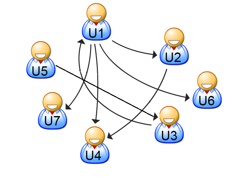
(a) User trust netwrok

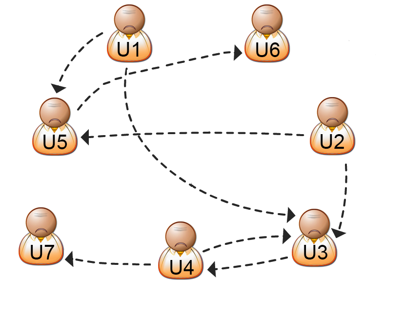
(b) User distrust netwrok

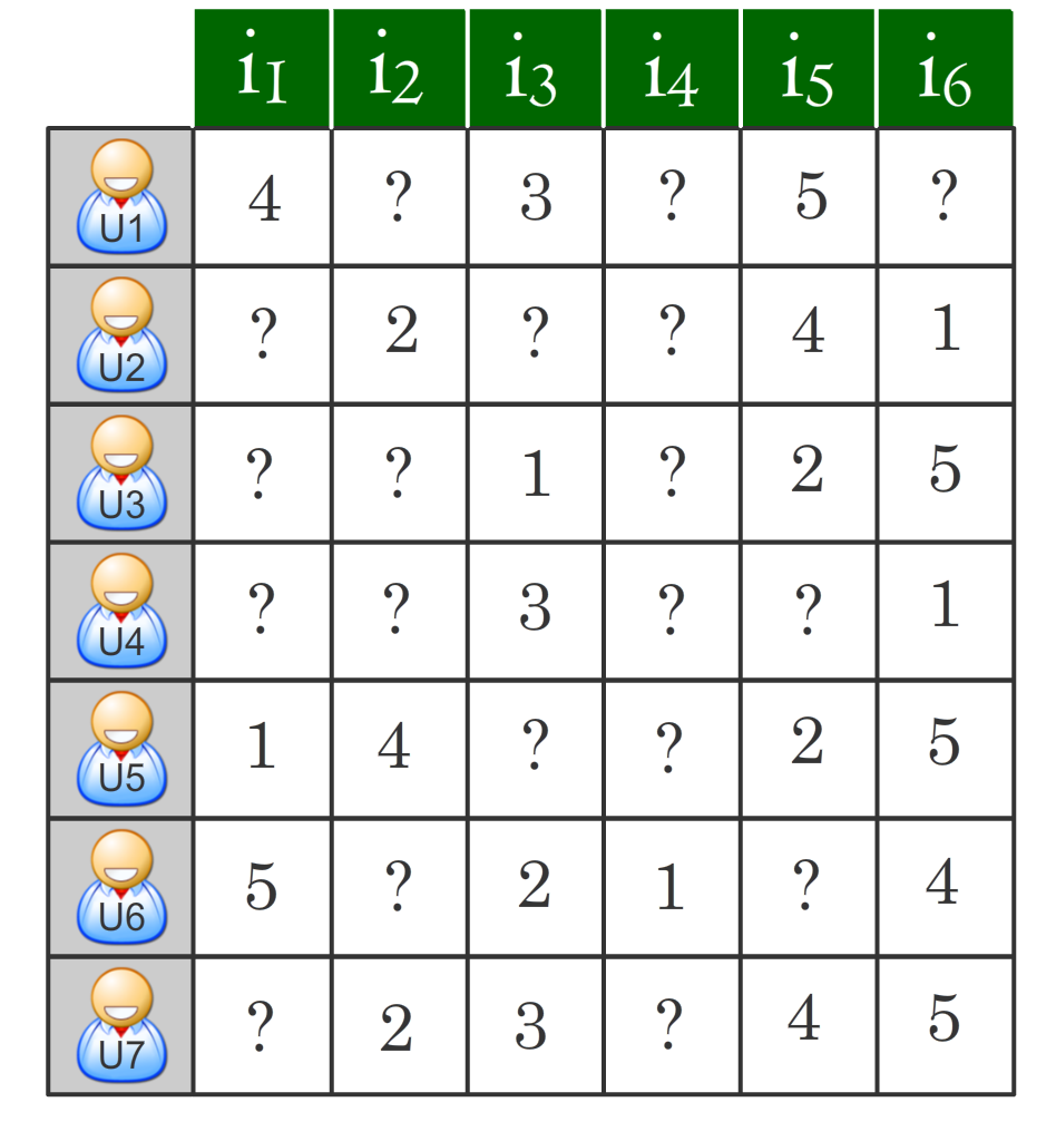
(c) Partially observed rating matrix

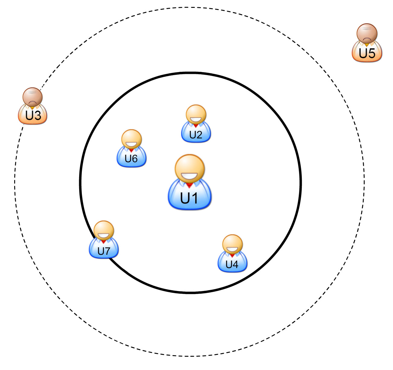
(d) Illustration of learned latent features

Figure 1: A simple example with seven users $\{u_{1},u_{2},\cdots,u_{7}\}$ and six items $\{i_{1},i_{2},\cdots,i_{6}\}$ to illustrate the main intuition behind the proposed algorithm. The inputs of the algorithm are (a) trust network, (b) distrust network, and (c) partially observed rating matrix $\mathbf{R}$, respectively. As shown in (d) for user $u_{1}$ , the learned latent features for all his trusted friends $\{u_{2},u_{4},u_{6},u_{7}\}$ are closer to $u_{1}$’s latent features than his distrusted friends $\{u_{3},u_{5}\}$ with a margin of 1.

Figure 1 shows an example to illustrate the intuition behind the mentioned idea. For ease of exposition, we only consider the latent features for the user $u_{1}$. From the trust network in Figure 1 (a) we can see that user $u_{1}$ trusts the list of users $\mathcal{N}_{+}=\{u_{2},u_{4},u_{6},u_{7}\}$ and from the distrust network in Figure 1 (b) we see that user $u_{1}$ distrusts the list of users $\mathcal{N}_{-}=\{u_{3},u_{5}\}$. The goal is to learn the latent features that obeys two goals, i) it minimizes the prediction error on observed entries in the rating matrix, ii) it respects the underlying structure of the trust and distrust networks between users. In Figure 1 (d) the latent features are depicted in the Euclidean space from the viewpoint of user $u_{1}$. As shown in Figure 1 (d), for user $u_{1}$, the latent features of his/her trusted friends $\mathcal{N}_{+}$ lie inside the solid circle centered at $u_{1}$ and the latent features of his/her distrusted friends $\mathcal{N}_{-}$ lie outside the dashed circle. The gap between two circles guarantees that always there exists a safe margin between $u_{1}$’s agreements with his trusted and distrusted friends. One simple way to impose these constraints on the latent features of users is to generate a set of triplets for any combination of trusted and distrusted friends ( e.g., one such triplet for user $u_{1}$ can be constructed as $(u_{1},u_{2},u_{5})$) and force the margin constraint to hold for all extracted triplets. This ensures that the minimum margin gap will definitely exist between the latent features of all the trusted and distrusted friends as desired and makes it possible to incorporate both types of relationships between users in the matrix factorization.

It is worthy to mention that similar to the social-enhanced recommender systems discussed before, the proposed algorithm is also based on hypotheses about the existence and the correlation of trust/distrust relations and ratings in the data. The empirical investigation of correlation between social relations and rating information has been the focus of a bulk of recent research including [83, 53, 38], where the results reinforce the hypothesis that ratings from trusted people count more than those from others and in particular distrusted neighbors. We have also conducted experiments as will be detailed in Subsection 5.5, to empirically investigate the correlation/alignment between social relations and the rating information issued by users which supports our strategy in exploiting the trust/distrust relations in matrix factorization.

We now formalize the proposed solution. As the first ingredient, we need a measure to evaluate the consistency between the latent features of users, i.e., the matrix $\mathbf{U}$, and the trust and distrust constraints existing between users in the social network. To this end, we introduce a monotonically increasing convex loss function $\ell(z)$ to measure the discrepancy between the latent features of different users. Let $u_{i}$, $u_{j}$, and $u_{k}$ be three users in the model such that $u_{i}$ trusts $u_{j}$ but distrusts $u_{k}$. The main intuition behind the proposed framework is that the latent features of $u_{i}$, i.e., $U_{i,:}$ must be more similar to $u_{j}$’s latent features than latent features for user $u_{k}$. For each such a triplet we penalize the objective function by $\ell(\mathcal{D}(U_{i,:},U_{j,:})-\mathcal{D}(U_{i,:},U_{k,:}))$ where the function $\mathcal{D}:\mathbb{R}^{k}\times\mathbb{R}^{k}\mapsto\mathbb{R}_{+}$ measures the similarity between two latent vectors assigned to two different users, and $\ell:\mathbb{R}\mapsto\mathbb{R}_{+}$ is a penalty function that is utilized to assess the violation of latent vectors of trusted and distrusted users. Example loss functions include hinge loss $\ell(z)=\max(0,1-z)$ and logistic loss $\ell(z)=\log(1+e^{-z})$ which are widely used convex surrogate of 0-1 loss function in learning community.

Let $\Omega_{\mathbf{S}}$ denote the set of extracted triplets from the social relations, i.e.,

$$\Omega_{\mathbf{S}}=\left\{(i,j,k)\in[n]\times[n]\times[n]:S_{ij}=1\;\;\&\;\;S_{ik}=-1\right\}.$$

Here, a positive relationship means friends or a trusted relationship and a negative relationship means foes or a distrust relationship. Then, our goal becomes to find a factorization of matrix $\mathbf{R}$ such that the learned latent features of users are consistent with the constraints in $\Omega_{\mathbf{S}}$ where the consistency is reflected in the loss function. This results in the following optimization problem:

$$\mathcal{L}(\mathbf{U},\mathbf{V}) =\frac{1}{2}\sum_{(i,j)\in\Omega_{\mathbf{R}}}{\left(R_{ij}-U_{i,:}^{\top}V_{j,:}\right)^{2}}+\frac{\lambda_{U}}{2}\|\mathbf{U}\|_{\rm{F}}+\frac{\lambda_{V}}{2}\|\mathbf{V}\|_{\rm{F}}$$

$$\hskip 14.22636pt+\frac{\lambda_{S}}{|\Omega_{\mathbf{S}}|}\sum_{(i,j,k)\in\Omega_{\mathbf{S}}}{\ell(\mathcal{D}(U_{i,:},U_{j,:})-\mathcal{D}(U_{i,:},U_{k,:}))}.$$ (4)

Let us make the above general formulation more specific by setting $\ell(\cdot)$ and $\mathcal{D}(\cdot,\cdot)$ to be the hinge loss and the Euclidian distance, respectively. Under these two assumptions, the objective can be formulated as:

$$\mathcal{L}(\mathbf{U},\mathbf{V}) =\underbrace{\frac{1}{2}\sum_{(i,j)\in\Omega_{\mathbf{R}}}{\left(R_{ij}-U_{i,:}^{\top}V_{j,:}\right)^{2}}}_{\mathcal{R}(\mathbf{U},\mathbf{V})}+\frac{\lambda_{U}}{2}\|\mathbf{U}\|_{\rm{F}}+\frac{\lambda_{V}}{2}\|\mathbf{V}\|_{\rm{F}}$$

$$\hskip 14.22636pt+\frac{\lambda_{S}}{|\Omega_{\mathbf{S}}|}\sum_{(i,j,k)\in\Omega_{\mathbf{S}}}{\max\left(0,1-\|U_{i,:}-U_{j,:}\|^{2}+\|U_{i,:}-U_{k,:}\|^{2}\right)}.$$ (5)

Here the constraints have been written in terms of hinge-losses over triplets, each consisting of a user, his/her trusted friend and his/her distrusted friend. Solving the optimization problem in (4.1) outputs the latent features for users and items that can utilized to estimate the missing values in the user-item matrix. Comparing the formulation in (4.1) to the existing factorization-based methods discussed earlier reveals two main features of the proposed formulation. First, it aims to minimize the error on the observed ratings and to respect the inherent structure of the social network among the users. The trade-off between these two objectives is captured by the regularization parameter $\lambda_{S}$ which is required to be tuned effectively.

In a similar way, applying the logistic loss to the general formulation in (4.1) yields the following objective:

$$\mathcal{L}(\mathbf{U},\mathbf{V}) =\frac{1}{2}\sum_{(i,j)\in\Omega_{\mathbf{R}}}{\left(R_{ij}-U_{i,:}^{\top}V_{j,:}\right)^{2}}+\frac{\lambda_{U}}{2}\|\mathbf{U}\|_{\rm{F}}+\frac{\lambda_{V}}{2}\|\mathbf{V}\|_{\rm{F}}$$

$$\hskip 14.22636pt+\frac{\lambda_{S}}{|\Omega_{\mathbf{S}}|}\sum_{(i,j,k)\in\Omega_{\mathbf{S}}}{\log\left(1+\exp\left(\|U_{i,:}-U_{k,:}\|^{2}-\|U_{i,:}-U_{j,:})\|^{2}\right)\right)}.$$ (6)

Remark 1.

We note that in several applications of recommender systems, besides the observed ratings, a description of the users and/or the objects through attributes (e.g., gender, age) or measures of similarity is available that could potentially benefit the process of recommendation (see e.g. [2] for few interesting applications). In that case it is tempting to take advantage of both known ratings and descriptions to model the preferences of users. A natural way to incorporate the available meta-data is to kernalize the similarity measure between latent features based on a positive definite kernel between pairs that can be deduced from the meta-data. More specifically, instead of simply using Euclidian distance as the similarity measure between latent features in (4.1), we can use the kernel matrix $\mathbf{K}$ obtained from the Laplacian of the graph obtained from the meta-data to measure the similarity as:

$$\mathcal{D}(U_{i,:},U_{j,:})=\left(U_{i,:}-U_{j,:}\right)^{\top}\mathbf{K}\left(U_{i,:}-U_{j,:}\right),$$

where $\mathbf{K}=(\mathbf{D}-\mathbf{W})^{-1}$, with $\mathbf{D}$ as a diagonal matrix with $D_{i,i}=\sum_{j=1}^{n}{W_{ij}}$. Here $\mathbf{W}$ captures the pairwise weight between users in the similarity graph between users that is computed based on the available meta-data about users.

Algorithm 1 GD based Matrix Factorization with Trust and Distrust Propagation

1:  Input: $\mathbf{R}$: partially observed rating matrix, $\Omega_{\mathbf{S}}$

2:  Output: $\mathbf{U}$ and $\mathbf{V}$

3:  for $t=1,\ldots,T$ do

4:     Compute the gradients $\nabla_{\mathbf{U}}\mathcal{R}(\mathbf{U}_{t},\mathbf{V}_{t})$ and $\nabla_{\mathbf{V}}\mathcal{R}(\mathbf{U}_{t},\mathbf{V}_{t})$.

5:     Compute $\nabla_{\mathbf{U}}$ by Eq. 7

6:     Compute $\nabla_{\mathbf{V}}$ by Eq. 8

7:     Update:

$$\mathbf{U}_{t+1}=\mathbf{U}_{t}-\eta_{t}\nabla_{\mathbf{U}}|_{\mathbf{U}=\mathbf{U}_{t},\mathbf{V}=\mathbf{V}_{t}}$$

$$\mathbf{V}_{t+1}=\mathbf{V}_{t}-\eta_{t}\nabla_{\mathbf{V}}|_{\mathbf{U}=\mathbf{U}_{t},\mathbf{V}=\mathbf{V}_{t}}$$

8:  end for

9:  return $\mathbf{U}_{T+1}$ and $\mathbf{V}_{T+1}$.

Remark 2.

We would like to emphasize that it is straightforward to generalize the proposed framework to incorporate similarity and dissimilarity information between items. What we need is to extract the triplets from the trust/distrust links between items and repeat the same process we did for users. This will add another term to the objective in terms of latent features of items $\mathbf{V}$ as shown in the following generalized formulation:

$$\mathcal{L}(\mathbf{U},\mathbf{V}) ={\frac{1}{2}\sum_{(i,j)\in\Omega_{\mathbf{R}}}{\left(R_{ij}-U_{i,:}^{\top}V_{j,:}\right)^{2}}}+\frac{\lambda_{U}}{2}\|\mathbf{U}\|_{\rm{F}}+\frac{\lambda_{V}}{2}\|\mathbf{V}\|_{\rm{F}}$$

$$\hskip 14.22636pt+\frac{\lambda_{S}}{|\Omega_{\mathbf{S}}|}\sum_{(i,j,k)\in\Omega_{\mathbf{S}}}{\max\left(0,1-\|U_{i,:}-U_{j,:}\|^{2}+\|U_{i,:}-U_{k,:}\|^{2}\right)}$$

$$\hskip 14.22636pt+\frac{\lambda_{{I}}}{|\Omega_{\mathbf{I}}|}\sum_{(i,j,k)\in\Omega_{\mathbf{I}}}{\max\left(0,1-\|V_{i,:}-V_{j,:}\|^{2}+\|V_{i,:}-V_{k,:}\|^{2}\right)},$$

where $\lambda_{I}$ is the regularization parameter and $\Omega_{\mathbf{I}}$ is the set of triplets extracted from the similar/dissimilar links between items. The similarity/dissimilarity links between items can be constructed according to tags issued by users or associated with items, and categories. For example, if two items are attached with a same tag, there is a trust link between them and otherwise distrust link. Alternatively, trust/distrust links can be extracted by measuring similarity/dissimilarity based on the item properties or profile if provided. This can further improve the accuracy of recommendations.

4.2 Batch Gradient Descent based Optimization

In optimization for supervised machine learning, there exist two regimes in which popular algorithms tend to operate: the stochastic approximation regime, which samples a small data set per iteration, typically a single data point, and the batch or sample average approximation regime, in which larger samples are used to compute an approximate gradient. The choice between these two extremes outlines the well-known tradeoff between inexpensive noisy steps and expensive but more reliable steps. Two preliminary examples of these regimes are the Gradient Descent (GD) and the Stochastic Gradient Descent (SGD) methods, respectively. Both GD and SGD methods starts with some initial point, and iteratively updates the solution using the gradient information at intermediate solutions. The main difference is that GD requires a full gradient information at each iteration while SGD only requires an unbiased estimate of the full gradient which can be done by sampling

We now discuss the application of GD algorithm to solve the optimization problem in (4.1) as detailed in Algorithm 1. Recall that the objective function is not jointly convex in both $\mathbf{U}$ and $\mathbf{V}$. On the other hand, the objective is convex in one parameter by fixing the other one. Therefore, we follow an iterative method to minimize the objective. At each iteration, first by fixing $\mathbf{V}$, we take a step in the direction of the negative gradient for $\mathbf{U}$ and repeat the same process for $\mathbf{V}$ by fixing $\mathbf{U}$.

For the ease of exposition, we introduce further notation. For any triplet $(i,j,k)\in\Omega_{\mathbf{S}}$ we note that the $\|U_{i,:}-U_{j,:}\|^{2}-\|U_{i,:}-U_{k,:}\|^{2}$ can be written as ${\rm{Tr}}(\mathbf{C}\mathbf{U}^{\top}\mathbf{U})$ where ${\rm{Tr}}(\cdot)$ denotes the trace of the input matrix and $\mathbf{C}$ is a sparse auxiliary matrix defined for each triplet with all entries equal to zero except: $\mathbf{C}_{ik}=\mathbf{C}_{ki}=\mathbf{C}_{jj}=1$ and $\mathbf{C}_{kk}=\mathbf{C}_{ij}=\mathbf{C}_{ji}=-1$. Having defined this notation, we can write the objective in (4.1) as:

$$\mathcal{L}(\mathbf{U},\mathbf{V}) =\mathcal{R}(\mathbf{U},\mathbf{V})+\frac{\lambda_{U}}{2}\|\mathbf{U}\|_{\rm{F}}+\frac{\lambda_{V}}{2}\|\mathbf{V}\|_{\rm{F}}+\frac{\lambda_{S}}{|\Omega_{\mathbf{S}}|}\sum_{(i,j,k)\in\Omega_{\mathbf{S}}}{\max\left(0,1-{\rm{Tr}}(\mathbf{C}_{ij}^{k}\mathbf{U}^{\top}\mathbf{U})\right)}.$$

where $\mathbf{C}_{ij}^{k}$ is the $\mathbf{C}$ matrix defined above which is associated with triplet $(i,j,k)$. To apply the GD method, we need to compute the gradient of $\mathcal{L}(\mathbf{U},\mathbf{V})$ with respect to $\mathbf{U}$ and $\mathbf{V}$ which we denote by $\nabla_{\mathbf{U}}=\nabla_{\mathbf{U}}\mathcal{L}(\mathbf{U},\mathbf{V})$ and $\nabla_{\mathbf{V}}=\nabla_{\mathbf{V}}\mathcal{L}(\mathbf{U},\mathbf{V})$, respectively. We have:

$$\nabla_{\mathbf{U}}=\nabla_{\mathbf{U}}\mathcal{R}(\mathbf{U},\mathbf{V})+\lambda_{U}\mathbf{U}-\frac{\lambda_{S}}{|\Omega_{\mathbf{S}}|}\sum_{(i,j,k)\in\Omega_{\mathbf{S}}}{\mathbf{1}_{[{\rm{Tr}}(\mathbf{C}_{ij}^{k}\mathbf{U}^{\top}\mathbf{U})<1]}(\mathbf{U}\mathbf{C}_{ij}^{k{\top}}+\mathbf{U}\mathbf{C}_{ij}^{k})}$$ (7)

where $\mathbf{1}_{[\cdot]}$ is the indicator function which takes a value of one if its argument is true, and zero otherwise. Similarly for $\nabla_{\mathbf{V}}$ we have:

$$\nabla_{\mathbf{V}}=\nabla_{\mathbf{V}}\mathcal{R}(\mathbf{U},\mathbf{V})+\lambda_{V}\mathbf{V}$$ (8)

The main shortcoming of GD method is its high computational cost per iteration due to the gradient computation (i.e., step (7)) which is expensive when the size of social constraints $\Omega_{\mathbf{S}}$ is large. We note that the size of $\Omega_{\mathbf{S}}$ can be as large as $O(n^{3})$ by considering all triplets in the social graph. In the next subsection we provide an alternative solution to resolve this issue using the stochastic gradient descent and mini-batch SGD methods which are more efficient than the GD method in terms of the computational cost per iteration but with a slow convergence rate in terms of target approximation error.

Algorithm 2 Mini-SGD based Matrix Factorization with Trust and Distrust Propagation

1:  Input: $\mathbf{R}$: partially observed rating matrix, $\Omega_{\mathbf{S}}$, min batch size $B$

2:  Output: $\mathbf{U}$ and $\mathbf{V}$

3:  for $t=1,\ldots,T$ do

4:     $\nabla_{t}\leftarrow\mathbf{0}$

5:     for $b=1,\ldots,B$ do

6:        $(i,j,k)\leftarrow\;\text{Sample random triplet from}\;\;\Omega_{\mathbf{S}}$

7:        if $(1-\|U_{i,:}-U_{j,:})\|^{2}+\|U_{i,:}-U_{k,:}\|^{2}>0)$ then

8:           $\nabla_{t}\leftarrow\mathbf{U}_{t}\mathbf{C}_{ij}^{k}\mathbf{U}_{t}^{\top}$

9:        end if

10:     end for

11:     Compute the gradients $\nabla_{\mathbf{U}}\mathcal{R}(\mathbf{U}_{t},\mathbf{V}_{t})$ and $\nabla_{\mathbf{V}}\mathcal{R}(\mathbf{U}_{t},\mathbf{V}_{t})$.

12:     Update:

$$\mathbf{U}_{t+1}=\mathbf{U}_{t}-\eta_{t}\left(\nabla_{\mathbf{U}}\mathcal{R}(\mathbf{U}_{t},\mathbf{V}_{t})+\lambda_{U}\mathbf{U}_{t}+\frac{\lambda_{S}}{B|\Omega_{\mathbf{S}}|}\nabla_{t}\right)$$

13:     Update:

$$\mathbf{V}_{t+1}=\mathbf{V}_{t}-\eta_{t}\left(\nabla_{\mathbf{V}}\mathcal{R}(\mathbf{U}_{t},\mathbf{V}_{t})+\lambda_{V}\mathbf{V}_{t}\right)$$

14:  end for

15:  return $\mathbf{U}_{T+1}$ and $\mathbf{V}_{T+1}$.

4.3 Stochastic and Mini-batch Optimization

As discussed above, when the size of social network is very large, the size of $\Omega_{\mathbf{S}}$ may cause computational problems in solving the optimization problem in (4.1) using GD method. The reason is essentially the fact that computing the gradient at each iteration requires to go through all the triplets in $\Omega_{\mathbf{S}}$ which is infeasible for large networks. To alleviate this problem we propose a stochastic gradient based [52] method to solve the optimization problem. The main idea is to choose a fixed subset of triplets for gradient computation instead of all $|\Omega_{\mathbf{S}}|$ triplets at each iteration [10]. More specifically, at each iteration, we sample $B$ triplets uniformly at random from $\Omega_{\mathbf{S}}$ to compute the next solution. We note that this strategy generates unbiased estimates of the true gradient and makes each iteration of algorithm computationally more efficient compared to the full gradient counterpart. In the simplest case, SGD algorithm, only one triplet is chosen at each iteration to generate an unbiased estimate of the full gradient. We note that in practice SGD is usually implemented based on data shuffling, i.e., making the sequence of the training samples random and then training the model by going through the training samples one by one. An intermediate solution, known as mini-batch SGD, chooses a subset of triplets to compute the gradient. The promise is that by selecting more triplets at each iteration, on one hand the variance of stochastic gradients decreases promotional to the number of sampled triplets, and on the other hand the algorithm enjoys the light computational cost of basic SGD method.

The detailed steps of the algorithm are shown in Algorithm 2. The mini-batch SGD method improves the computational efficiency by grouping multiple constraints into a mini-batch and only updating the $\mathbf{U}$ and $\mathbf{V}$ once for each mini-batch. For brevity, we will refer to this algorithm as Mini-SGD. More specifically, the Mini-SGD algorithm, instead of computing the full gradient over all triplets, samples $B$ triplets uniformly at random from $\Omega_{\mathbf{S}}$ where $1\leq B\leq|\Omega_{\mathbf{S}}|$ is a parameter that needs to be provided to the algorithm, and computes the stochastic gradient as:

$$\nabla_{t}=\frac{\lambda_{S}}{B}\sum_{(i,j,k)\in\Omega_{B}}{\mathbf{1}_{[{\rm{Tr}}(\mathbf{C}_{ij}^{k}\mathbf{U}_{t}^{\top}\mathbf{U}_{t})<1]}(\mathbf{U}\mathbf{C}_{ij}^{k{\top}}+\mathbf{U}\mathbf{C}_{ij}^{k})}$$

where $\Omega_{B}$ is the set of $B$ sampled triplets from $\Omega_{\mathbf{S}}$. We note that

$$\mathbf{E}[\nabla_{t}]=\frac{\lambda_{S}}{|\Omega_{\mathbf{S}}|}\sum_{(i,j,k)\in\Omega_{\mathbf{S}}}{\mathbf{1}_{[{\rm{Tr}}(\mathbf{C}_{ij}^{k}\mathbf{U}_{t}^{\top}\mathbf{U}_{t})<1]}(\mathbf{U}\mathbf{C}_{ij}^{k{\top}}+\mathbf{U}\mathbf{C}_{ij}^{k})},$$

i.e., $\nabla_{t}$ is an unbiased estimate of the full gradient in the right hand side. When $B=|\Omega_{\mathbf{S}}|$, each iteration handles the original objective function and Mini-SGD reduces to the batch GD algorithm. We note that both GD and SGD share the same convergence rate in terms of number of iterations in expectation for non-smooth optimization problems (i.e., $O(1/\sqrt{T})$ after $T$ iterations), but SGD method requires much less running time to convergence compared to the GD method due to the efficiency of its individual iterations.

5 Experimental Results

In this section, we conduct exhaustive experiments to demonstrate the merits and advantages of the proposed algorithm. We conduct the experiments on the well-known Epinions  data set, aiming to accomplish and answer the following fundamental questions:

1. Prediction accuracy: How does the proposed algorithm perform in comparison to the state-of- the-art algorithms with/without incorporating trust and distrust relationships between users. Whether or not the trust/distrust social network could help in making more accurate recommendations?

2. Correlation of social relations with rating information: To what extent, the trusted and distrusted friends of a user $u$ are aligned with the ratings the user $u$ issued for the reviews written by his friends? A positive answer to this question indicates that two users will issue similar (dissimilar) ratings if they are connected by a trust (distrust) relation and prefer to behave similarly.

3. Model selection: What role do the regularization parameters $\lambda_{S}$, $\lambda_{U}$ and $\lambda_{V}$ play in the accuracy of the proposed recommender system and what is the best strategy to tune these parameters?

4. Handling cold-start users: How does exploiting social relationships in prediction process affect the performance of recommendation for cold-start users?

5. Trading trust for distrust: To what extent the distrust relations can compensate for the lack of trust relations?

6. Efficiency of optimization: What is the trade-off between accuracy and efficiency by moving from the gradient descent to the stochastic gradient descent with different batch sizes?

In the following subsections, we intend to answer these questions. We begin by introducing the data set we use in our experiemnts and the metrics we employ to evaluate the results, followed by the detailed experimental results.

5.1 Data Set Description and Experimental Setup

The Epinions data set

We begin by discussing the data set we have chosen for our experiments. To evaluate the proposed algorithm on trust and distrust-aware recommendations, we use the Epinions data set [22], a popular e-commerce site and customer review website where users share opinions on various types of items such as electronic products, companies, and movies, through writing reviews about them or assigning a rating to the reviews written by other users. The rating values in Epinions are discrete values ranging from Ònot helpfulÓ (1/5) to Òmost helpfulÓ (5/5). These ratings and reviews would potentially influence future customers when they are about to decide whether a product is worth buying or a movie is worth watching.

Epinions allows users to evaluate other users based on the quality of their reviews, and to make trust and distrust relations with other users in addition to the ratings. Every member of Epinions can maintain a "trust" list of people he/she trusts that is referred to as web of trust (social network with trust relationships) based on the reviewers with consistent ratings or "distrust" list known as block list (social network with distrust relationships) that presents reviewers whose reviews were consistently found to be inaccurate or low quality. The fact that the data set contains explicit positive and negative relations between users makes it very appropriate to study issues in trust- and distrust-enhanced recommender systems. Epinions is thus an ideal source for experiments on social recommendation. We remark that the Epinions data set only contains bivalent relations (i.e., contains only full trust and full distrust, and no gradual statements).

To conduct the coming experiments, we sampled a subset of Epinions data set with $n=121,240$ users and $m=685,621$ different items. The total number of observed ratings in the sampled data set is 12,721,437 which approximately includes $0.02\%$ of all entries in the rating matrix $\mathbf{R}$ which demonstrates the sparsity of the rating matrix. We note that the selected items are the most frequently rated overall. The statistics of the data set is given in Table 2. The social statistics of the this data source is summarized in Table 3. The frequencies of ratings for users is shown are Table 4. In the user distrust network, the total number of issued distrust statements is 96,823. As to the user trust network, the total number of issued trust statements is 481,799.

Experimental setup

To better evaluate the effect of utilizing the social side information in recommendation accuracy, we employ different amount of training data 90%, 80% , 70% and 60% to create four different training sets that are increasingly sparse but the social network remains the same in all of them. Training data 90%, for example, means we randomly select 90% of the ratings from the sampled Epinions data set as the training data to predict the remaining 10% of ratings. The random selection was carried out $5$ times independently to have a fair comparison. Also, since our preliminary results on a smaller data set revealed that the hinge loss performs better than the exponential loss, in the rest of experiments we stick to this loss function. However, we note the exponential loss is slightly faster in optimizing the corresponding objective function thanks to its smoothness, but it was negligible considering its worse accuracy compared to the hinge loss. All implementations are in Matlab, and all experiments were performed on a 4-core 2.0 GHZ of a load-free machine with a 12G of RAM.

Table 2: Statistics of sample data from Epinions data set used in our experiments.

Statistic	Quantity
Number of users	121,240
Number of items	685,621
Number of ratings	12,721,437
Number of trust relations	481,799
Number of distrust relations	96,823
Minimum number of ratings by users	1
Minimum number of ratings for items	1
Maximum number of ratings by users	148735
Maximum number of ratings for items	945
Average number of ratings by users	85.08
Average number of ratings for items	15.26

Table 3: Maximum and average trust and distrust relations for users in the sampled data set.

Statistics	Trust per user	Be Trusted per user
Max	1983	2941
Min	1	0
Average	4.76	4.76
	Distrust per user	Be Distrusted per user
Max	1188	429
Min	1	0
Average	0.91	0.91

Table 4: The frequencies of user’s rating.

# of Ratings	0-10	11-20	21-30	31-40	41-50	$51-60$
# of Users	4,198,074 ($\approx 33\%$)	3,053,144 ($\approx 24\%$)	2,289,858 ($\approx 18\%$)	1,526,572 ($\approx 12\%$)	534,300 ($\approx 4.2\%$)	267,150 ($\approx 2.1\%$)
# of Ratings	61-70	71-80	81-90	91-100	101-200	$201-300$
# of Users	157,745 ($\approx 1.24\%$)	143,752 ($\approx 1.13\%$)	104,315 ($\approx 0.82\%$)	43,252 ($\approx 0.34\%$)	21,626 ($\approx 0.17\%$)	10,686 ($\approx 0.084\%$)

5.2 Metrics

5.2.1 Metrics for rating prediction

We employ two well-known measures, the Mean Absolute Error (MAE) and the Root Mean Squared Error (RMSE) [25] to measure the prediction accuracy of the proposed approach in comparison with other basic collaborative filtering and trust/distrust-enhanced recommendation methods.

MAE is very appropriate and useful measure for evaluating prediction accuracy in offline tests [25, 45]. To calculate MAE, the predicted rating is compared with the real rating and the difference (in absolute value) considered as the prediction error. Then, these individual errors are averaged over all predictions to obtain the overall MAE value. More precisely, let $\mathcal{T}$ denote the set of ratings to be predicted, i.e., $\mathcal{T}=\{(i,j)\in[n]\times[m],R_{ij}\;\text{needs to be predicted}\}$ and let $\hat{\mathbf{R}}$ denote the prediction matrix obtained by algorithm after factorization. Then,

$${\rm{MAE}}=\frac{\sum_{(i,j)\in\mathcal{T}}{{|R_{ij}-\hat{R}_{ij}|}}}{|\mathcal{T}|},$$

where ${R}_{ij}$ is the real rating assigned by the user $i$ to the item $j$, and $\hat{R}_{ij}$ is the rating user $i$ would assign to the item $j$ that is predicted by the algorithm .

The RMSE metric is defined as:

$${\rm{RMSE}}=\sqrt{\frac{\sum_{(i,j)\in\mathcal{T}}{{\left(R_{ij}-\hat{R}_{ij}\right)^{2}}}}{|\mathcal{T}|}}.$$

The first measure (MAE) considers every error of equal value, while the second one (RMSE) emphasizes larger errors. We would like to emphasize that even small improvements in RMSE are considered valuable in the context of recommender systems. For example, the Netflix prize competition offered a 1,000,000 reward for a reduction of the RMSE by 10% [72].

5.2.2 Metrics for evaluating the correlation of ratings with trust/distrust relations

As part of our experiments, we investigate how the explicit trust/distrust relations between users in the social network are aligned with the implicit trust/distrust relations between users conveyed from the rating information. We use recall, Mean Average Precision (MAP) [44] and Normalized Discount Cumulative Gain (NDCG) to evaluate the ranking results. Recall is defined as the number of relevant friends divided by the total number of friends in the social network. Precision is defined as the number of relevant friends (trusted or distrusted) divided by the number of friends in the social network. Given a user $u$, let $r_{i}$ be the relevance score of the friend ranked at position $i$, where $r_{i}=1$ if the user is relevant to the $u$ and $r_{i}=0$ otherwise. Then we can compute the Average Precision (AP) as

$${\rm{AP}}=\frac{\sum_{i}{r_{i}\times{\rm{Precision}}@i}}{\#\text{ of relevant friends}}.$$

MAP is the average of AP over all the users in the network.

NDCG is a normalization of the Discounted Cumulative Gain (DCG) measure. DCG is a weighted sum of the degree of relevancy of the ranked users. The weight is a decreasing function of the rank (position) of the user, and therefore called discount. NDCG normalizes DCG by the Ideal DCG (IDCG), which is simply the DCG measure of the best ranking result. Thus NDCG measure is always a number in $[0,1]$. NDCG at position $k$ is defined as:

$${\rm{NDCG}}@k=Z_{k}\sum_{i=1}^{k}{\frac{2^{r_{i}}-1}{\log(i+1)}}$$

where $k$ is also called the scope, which means the number of top-ranked users presented to the user and $Z_{k}$ is chosen such that the perfect ranking has a NDCG value of 1. We note that the base of the logarithm does not matter for NDCG, since constant scaling will cancel out due to normalization. We will assume it is the natural logarithm throughout this paper.

Figure 2: Grid Search to find the best values for $\lambda_{U}$ and $\lambda_{C}$ on the data set with 90% of rating information.

5.3 Model Selection

Tuning of parameters (a.k.a model selection in learning community) is a critical problem in most of the learning problems. In some situations, the learning performance may drastically vary with different choices of the parameters. There are three parameters in objective (4.1) that play very important role in the effectivity of the proposed algorithm. These are $\lambda_{U}$, $\lambda_{V}$, and $\lambda_{S}$. Between these, $\lambda_{S}$ controls how much the proposed algorithm should incorporate the information of the social network in completing the partially observed rating matrix. In the extreme case, a very small value for $\lambda_{S}$, the algorithm almost forgets the social information exists between the users and only utilizes the observed user-item rating matrix for factorization. On the other hand, if we employ a very large value for $\lambda_{S}$, the social network information will dominate the learning process, leading to a poorer performance. Therefore, in order to not hurt the recommendation performance, we need to find a reasonable value for social regularization parameter. To this end, we analyze how the combination of these parameters affect the recommendation performance.

We conduct a grid search on the potential values of two parameters $\lambda_{S}$ and $\lambda_{V}$ to find the combination with best performance. Figure 2 shows the grid search results for these parameters on data set with 90% of training data where the optimal prediction accuracy is achieved at point $(14.8,11)$ with the optimal $\mbox{RMSE}=1.12$. We would like to emphasize that we have done the cross validation for only pairs of $(\lambda_{S},\lambda_{V})$ and $(\lambda_{S},\lambda_{U})$ because, (i) considering the grid search for the triplet $(\lambda_{S},\lambda_{U},\lambda_{V})$ is computationally burdensome, (ii) and our preliminary experiments showed that $\lambda_{V}$ and $\lambda_{U}$ behave similarly with respect to $\lambda_{S}$. Based on the results reported in Figure 2, in the remaining experiments, we set $\lambda_{S}=14.8$, $\lambda_{V}=11$, and $\lambda_{U}=13$ when the training is performed on the data set with 90% of rating information. We repeat the same process to find out the best setting of regularization parameters for other data sets with 80%, 70%, and 60% of rating data as well.

5.4 Baseline Methods

Here we briefly discuss the baseline algorithms that we intend to compare the proposed algorithm. The baseline algorithms are chosen from both types of memory-based and model-based recommender systems with different types of trust and distrust relations. In particular, we consider the following basic algorithms:

• MF (matrix factorization based recommender): this is the basic matrix factorization based recommender formulated in the optimization problem in (1) which does not take the social data into account.

• MF+T (matrix factorization with trust information): to exploit the trust relations between users in matrix factorization, [40] relied on the fact that the distance between latent features of users who trust each other must be minimized that can be formulated as the following objective:

  $$\min_{\mathbf{U}}\frac{1}{2}\sum_{i=1}^{n}\sum_{j\in{\mathcal{N}}_{+}(i)}{\mathcal{D}(U_{i,:},U_{j,:})},$$

  where ${\mathcal{N}}_{+}(i)$ is the set of users the $i$th user trusts in the social network (i.e., $S_{ij}=+1$). By employing this intuition in the basic formulation in (1), [40] solves the following optimization problem:

  $$\min_{\mathbf{U},\mathbf{V}}\left[\frac{1}{2}\sum_{(i,j)\in\Omega_{\mathbf{R}}}{\left(R_{ij}-U_{i,:}^{\top}V_{j,:}\right)^{2}}+\frac{\alpha}{2}\sum_{i=1}^{n}\sum_{j\in\mathcal{N}_{+}(i)}{\mathcal{D}(U_{i,:},U_{j,:})}+\frac{\lambda_{U}}{2}\|\mathbf{U}\|_{\rm{F}}+\frac{\lambda_{V}}{2}\|\mathbf{V}\|_{\rm{F}}\right].$$

• MF+D (matrix factorization with distrust information): the basic intuition behind the algorithm proposed in [40] to exploit the distrust relations is as follows: if user $u_{i}$ distrusts user $u_{j}$, then we can assume that their corresponding latent features $U_{i,:}$ and $U_{j,:}$ would have a large distance. As a result we aim to maximize the following quantity for all users:

  $$\max_{\mathbf{U}}\frac{1}{2}\sum_{i=1}^{n}\sum_{j\in\mathcal{N}_{-}(i)}{\mathcal{D}(U_{i,:},U_{j,:})},$$

  where $\mathcal{N}_{-}(i)$ denotes the set of users the $i$th users distrusts (i.e, $S_{ij}=-1$). Adding this term to the basic optimization problem in (1) we obtain the following optimization problem:

  $$\min_{\mathbf{U},\mathbf{V}}\left[\frac{1}{2}\sum_{(i,j)\in\Omega_{\mathbf{R}}}{\left(R_{ij}-U_{i,:}^{\top}V_{j,:}\right)^{2}}-\frac{\beta}{2}\sum_{i=1}^{n}\sum_{j\in\mathcal{N}_{-}(i)}{\mathcal{D}(U_{i,:},U_{j,:})}+\frac{\lambda_{U}}{2}\|\mathbf{U}\|_{\rm{F}}+\frac{\lambda_{V}}{2}\|\mathbf{V}\|_{\rm{F}}\right].$$

• MF+TD (matrix factorization with trust and distrust information): this algorithm stands for the algorithm proposed in the present work. We note that there is no algorithm in the literature that exploits both trust and distrust relations in factorization process simultaneously.

• NB (neighborhood-based recommender): this algorithm is the basic memory-based recommender algorithm that predicts a rating of a target item $i$ for user $u$ using a combination of the ratings of neighbors of $u$ (similar users) that already issued a rating for item $i$. Formally,

  $$\hat{R}_{ui}=\bar{R}_{u}+\frac{\sum_{u^{\prime}\in\mathcal{N}(u),W_{uu^{\prime}}>0}{W_{uu^{\prime}}(R_{ui}-\bar{R}_{u})}}{\sum_{u^{\prime}\in\mathcal{N}(u),W_{uu^{\prime}}}{W_{uu^{\prime}}}},$$ (9)

  where the pairwise weight $W_{uu^{\prime}}$ between pair of users $(u,u^{\prime})$ is calculated by Pearson’s correlation coefficient [25]

• NB+T (neighborhood with trust information) [45, 17, 47]: the basic idea behind the trust based recommender systems proposed in TidalTrsut [17] and MoleTrsut [45] is to limit the set of neighbors in (9) to the users who are trusted by user $u$. The distinguishing feature of these algorithms is the mechanism of trust propagation to estimate the trust transitively for all the users. By adapting (9) to only consider trustworthy neighbors in predicting the new ratings we obtain:

  $$\hat{R}_{ui}=\bar{R}_{u}+\frac{\sum_{u^{\prime}\in\mathcal{N}^{*}_{+}(u),W_{uu^{\prime}}>0}{W_{uu^{\prime}}(R_{ui}-\bar{R}_{u})}}{\sum_{u^{\prime}\in\mathcal{N}^{*}_{+}(u),W_{uu^{\prime}}>0}{W_{uu^{\prime}}}},$$ (10)

  where $\mathcal{N}^{*}_{+}(u)$ is the set of trusted neighbors of $u$ in the social network with propagated trust relations (when there is no propagation we have $\mathcal{N}^{*}_{+}(u)=\mathcal{N}_{+}(u)$). We note that instead of Pearson’s correlation coefficient as the wighting schema, we can infer the weights exploiting the social relation between the users. Since for the data set we consider in our experiments, the trust/distrust relations are binary values, the social based pairwise distance would be simply the hamming distance between the binary vector representation of social relations of users. For implementation details we refer to [70, Chapter 6].

• NB+TD-F (neighborhood with trust information and distrust information as filtration) [69, 72]: a simple strategy to use distrust relations in the recommendation is to filter out distrusted users from the list of neighbors in predicting the ratings. As a result, we adapt (9) to exclude distrusted users from the users’ propagated web of trust.

• NB+TD-D (neighborhood-based with trust information and integrated distrust information) [69, 72]: in the same spirit as the filtration strategy, we can use distrust relations to debug the trust relations. More specifically, if user $u$ trusts user $v$, $v$ trusts $w$, and $u$ distrusts $w$, then the latter distrust relation contradicts the propagation of the trust from $u$ to $w$ and can be excluded from the prediction. In this method distrust is used to debug the trust relations.

Table 5: The consistency of implicit and explicit trust relations in the data set for different ranges of ratings measured in terms of NDCG, recall, and MAP.

# of Ratings	NDCG@10	NDCG@20	Recall@10	Recall@20	Recall@40	MAP
0-20	0.083	0.078	0.054	0.092	0.156	0.140
21-40	0.108	0.103	0.080	0.125	0.198	0.190
41-60	0.117	0.112	0.083	0.128	0.225	0.208
61-80	0.120	0.117	0.088	0.132	0.230	0.230
$\geq 81\;$	0.135	0.126	0.091	0.151	0.253	0.244

Table 6: The consistency of implicit and explicit distrust relations in the data set for different ranges of ratings measured in terms of NDCG, recall, and MAP.

# of Ratings	NDCG@10	NDCG@20	Recall@10	Recall@20	Recall@40	MAP
0-20	0.065	0.057	0.045	0.071	0.132	0.130
21-40	0.071	0.068	0.060	0.077	0.140	0.134
41-60	0.082	0.072	0.075	0.085	0.158	0.152
61-80	0.089	0.078	0.081	0.105	0.164	0.160
$\geq 81\;$	0.104	0.096	0.087	0.125	0.191	0.183

5.5 On the Consistency of Social Relations and Rating Information

As already mentioned, the Epinions website allows users to write reviews about products and services and to rate reviews written by other users. Epinions also allows users to define their web of trust, i.e. "reviewers whose reviews and ratings have been consistently found to be valuable" and their block list, i.e. "reviewers whose reviews are found to be consistently inaccurate or not valuableÓ. Different intuitions on interpreting these social information will result in different models. The main rational behind incorporating trust and distrust relations in recommendation process is to take the trust/distrust relations between users in the social network as the level of agreement between ratings assigned to reviews by users . Therefore, investigating the consistency or alignment between user ratings (implicit trust) and trust/distrust relations in the social network (explicit trsut) become an important issue.

Here, we aim to empirically investigate whether or not there is a correlation between a user’s current trustees/friends or distrusted friends and the ratings that user would assign to reviews issued by his neighbors. Obviously, if there is no correlation between social context of a user and his/her ratings to reviews written by his neighbors, then the social structure does not provide any advantage to the rating information. On the other hand, if there exists such a correlation, then the social context could be supplementary information to compensate for the lack of rating information to boost the accuracy of recommendations.

The consistency of trust relations and rating information issued by users on the reviews written by his trustees has been analyzed in [83, 23]. However, [83] also claimed that social trust (i.e., explicit trust) and similarity between users based on their issued ratings (i.e., implicit trust) are not the same, and can be used complementary. According to [38], when comparing implicit social information with explicit social information, the performance of using implicit information is slightly worse. We further investigate the same question about the consistency of distrust relations and ratings issued by users to their distrusted neighbors. The positive answer to this question can be interpreted as follows. Given that user $u$ is interested in item $i$, the chances that $v$, trusted (distrusted) by $u$, also likes this item $i$ is much higher (lower) than for user $w$ not explicitly trusted (distrusted) by $u$.

To measure the similarity between users, there are several methods we can borrow in the literature. In this paper, we adopt the most popular approach that is referred to as Pearson correlation coefficient (PCC) $\mathcal{P}:\mathcal{U}\times\mathcal{U}\mapsto[-1,+1]$ [6, 47], which is defined as:

$$\mathcal{P}(u,v)=\frac{\sum_{i=1}^{m}{(R_{ui}-\bar{R}_{u})(R_{vi}-\bar{R}_{v})}}{\sqrt{\sum_{j=1}^{m}{(R_{ui}-\bar{R}_{u})^{2}}\times\sum_{j=1}^{m}{(R_{vi}-\bar{R}_{v})^{2}}}},\forall u,v\in\mathcal{U},$$

where $\bar{R}_{u}$ and $\bar{R}_{v}$ are the average of ratings issued by users $u$ and $v$, respectively. The PCC measures the extent to which there is a linear relationship between the rating behaviors of the two users, the extreme values being -1 and 1. The similarity of two users becomes negative when users have completely diverging ratings. We note that this quantity can be considered as the implicit trust between users that is conveyed via ratings given by users.

Table 7: The alignment rate of users in establishing trust/distrust relationships with future users in the social network based on the majority vote of their current trusted/distrusted friends. The number of trusted friends (+) and distrusted friends (-) are denoted by $n_{+}$ and $n_{-}$, respectively. Here $u$ denotes the current user and $w$ stands for a future user in the network.

Setting	Type of Relation ($u\leadsto w$)	% of Relations	Alignment Rate (%)
$n_{+}>n_{-}$	+	48.80	92.09
	-	2.54	8.15
$n_{+}<n_{-}$	+	1.15	17.88
	-	8.02	83.42
$n_{+}=n_{-}>0$ or $n_{+}=n_{-}=0$	+	39.49	-

To conduct this set of experiments, we first group all the users in the training data set based on the number of ratings, and then measure the prediction accuracies of different user groups. Users are grouped into five classes: "[1, 20)", "[20, 40)", "[40, 60)", "[60, 80)", and "$>81$ ". In order to have a comprehensive view of the ranking performance, we present the NDCG, recall and MAP scores of trust and distrust alignments on the Epinions data set in Table 5 and Table 6, respectively. We note that the data set we use in our experiments only contains bivalent trust values, i.e., -1 and +1, and it is not possible to have an ordering on the list of friends (timestamp of relations would be an option to order the friends but unfortunately it is not available in our data set). To compute the NDCG, we use the ordering of trusted/distrusted friends which yields the best value.

On the positive side, we observe a clear trend of alignment between ratings assigned by a user and the type of relation he has made in the social network. This observation coincides with our intuition. Overall, when more ratings are observed for a user, the similarity calculation process will find more accurate similar or dissimilar neighbors for this user since we have more information to represent or interpret this user. Hence, by increasing the number of ratings, It is conceivable from the results in Tables 5 and 6 that the alignment between implicit and explicit neighbors becomes better. By comparing the results in Tables 5 and 6 we can see that trust relations are slightly better aligned than the distrust relations.

On the negative side, the results show that the NDCG on both types of relations is small. One explanation for this phenomenon is that the Epinions data set is not tightly bound to a specific application. For example, a user may trust or distrust anther user based on his/her comments on a specific product but they might have similar taste on other products. Furthermore, compared to other data sets such as FilmTrusts, the Epinions data set is very sparse data set, and consequently it is relatively inaccurate to rely on the rating information to compute the implicit trust relations. Finally, our approach to distinguish trust/distrust lists from the rating information is limited by the PCC trust metric we have utilized. We conjecture that better trust metrics that is able to exploit other side information such as time and interactional information would be helpful in distinguishing implicit trusted/distrusted friends, leading to better alignment between implicit and explicit trust relations.

We also conduct experiments to evaluate the consistency of social network only based on the trust/distrust relations between users. In particular, we investigate to what extent a users’ relations are aligned with the opinion of his/her neighbors in the social network. More specifically, let $u$ be a user who is about to make a trust or distrust relation to another user $v$. We assume that $n_{+}$ number of $u$’s neighbors trust $v$ and $n_{-}$ number of $u$’s neighbors distrust $v$. We note that in the real data set the distrust relations are hidden. To conduct this set of experiments, we randomly sample 30% of the relations from the social network and use the remaining 70% to predict the type of sampled relations  by majority voting.

Table 7 shows the results on the consistency of social relations. We observe that in all cases there is an alignment between the opinions of users’ friends and his/her own relation (92.09% and 83.42% when the majority of friends trust and distrust the target user, respectively). This might be due to social influence of people on social network, however, it is hard to justify the existence of such a correlation in Epinions data set which includes reviews for diverse set of products and taste of users. One interesting observation from the results reported in Table 7 is the case where the number of distrusted users dominates the number of trusted users (i.e., $n_{-}>n_{+}$). While the distrust relations are private to other users, but we can see that there is a significant alignment between users’s relation type and his distrusted friends.

Table 8: The accuracy of prediction of matrix factorization with three different methods measured in terms of MAE and RMSE errors. The parameter $k$ represents the number of latent features in factorization.

$k$	$\%$ of Training	Measure	MF	MF+T	MF+D	MF+TD
10	60%	MAE	0.9813 $\pm$ 0.042	0.8561 $\pm$ 0.032	0.9720 $\pm$ 0.038	0.8310 $\pm$ 0.016
		RMSE	1.6050 $\pm$ 0.032	1.4125 $\pm$ 0.022	1.5036 $\pm$ 0.040	1.2294 $\pm$ 0.086
	70%	MAE	0.9462 $\pm$ 0.083	0.8332 $\pm$ 0.092	0.9241 $\pm$ 0.012	0.8206 $\pm$ 0.023
		RMSE	1.5327 $\pm$ 0.032	1.2407 $\pm$ 0.063	1.4405 $\pm$ 0.023	1.1562 $\pm$ 0.043
	80%	MAE	0.9150$\pm$ 0.022	0.8206 $\pm$ 0.041	0.8722 $\pm$ 0.034	0.8113 $\pm$ 0.032
		RMSE	1.3824 $\pm$ 0.032	1.1906 $\pm$ 0.042	1.3155 $\pm$ 0.026	1.1061 $\pm$ 0.021
	90%	MAE	0.8921 $\pm$ 0.025	0.8158 $\pm$ 0.016	0.8736 $\pm$ 0.053	0.8025 $\pm$ 0.014
		RMSE	1.2166 $\pm$ 0.017	1.1403 $\pm$ 0.027	1.1869 $\pm$ 0.049	1.0872 $\pm$ 0.020
20	60%	MAE	0.9972 $\pm$ 0.016	0.8431 $\pm$ 0.018	0.9746 $\pm$ 0.060	0.8475 $\pm$ 0.012
		RMSE	1.6248 $\pm$ 0.014	1.3904 $\pm$ 0.042	1.5423 $\pm$ 0.046	1.1837 $\pm$ 0.023
	70%	MAE	0.9688 $\pm$ 0.019	0.8342 $\pm$ 0.062	0.9350 $\pm$ 0.022	0.8290 $\pm$ 0.034
		RMSE	1.5162 $\pm$ 0.016	1.2722 $\pm$ 0.027	1.4540 $\pm$ 0.075	1.1452 $\pm$ 0.016
	80%	MAE	0.9365 $\pm$ 0.025	0.8172 $\pm$ 0.011	0.8705 $\pm$ 0.016	0.8129 $\pm$ 0.025
		RMSE	1.4081 $\pm$ 0.015	1.1853 $\pm$ 0.023	1.3591 $\pm$ 0.073	1.1049 $\pm$ 0.082
	90%	MAE	0.9224 $\pm$ 0.016	0.8128 $\pm$ 0.021	0.8805 $\pm$ 0.032	0.8096 $\pm$ 0.010
		RMSE	1.2207 $\pm$ 0.0 18	1.1402 $\pm$ 0.026	1.1933 $\pm$ 0.028	1.0851 $\pm$ 0.011

5.6 On the Power of Utilizing Social Relationships

We now turn to investigate the effect of utilizing social relationships between users on the accuracy of recommendations in factorization-based methods. In other words, we would like to experimentally evaluate whether incorporating distrust can indeed enhance the trust-based recommendation process. To this end, we run four different MF (i.e., pure matrix factorization based algorithm), MF+T (i.e., matrix factorization with only trust relationships), MF+D (i.e., matrix factorization with only distrust relationships), and MF+TD (i.e., the algorithm proposed here) algorithms on the data set. We run the algorithms with $k=10$ and $k=20$ latent vector dimensions. As mentioned earlier, different amount of training data 90%, 80% , 70% and 60% has been used to create four different training sets that are increasingly sparse but the social network remains the same in all of them. We evaluate all algorithms by both MAE and RMSE measures.

Table 8 shows the MAE and RMSE errors for the four sampled data sets. First, as we expected, the performance of all learning algorithms improves with an increasing number of training data. It is also not surprising to see that the MF+T, MF+D, and MF+TD algorithms which exploit social side information perform better than the pure matrix factorization based MF algorithm. Second, the proposed algorithm outperforms all other baseline algorithms for all the cases, indicating that it is effective to incorporate both types of social side information in recommendation. This result by itself indicates that besides trust relationships in the social network, the distrust information is also a rich source of information and can be utilized in recommendation algorithms. We note that distrust information needs to be incorporated carefully as its nature is totally different from trust information. Finally, it is noticeable that the MF+T outperforms the MF+D algorithm due to huge number of trust relations to distrust relations in our data set. It is also remarkable that users are more likely to be influenced by their friends to make trust relations than the distrust relations due to the private nature of distrust relations in Epinions data set. This might lead us to believe that distrust relations have better quality than trust relations which requires a deeper investigation to be verified.

5.7 Comparison to Baseline Algorithms

Another question that is worthy of investigation is how state-of-the-art approaches perform compared to the method proposed in this paper. To this end, we compare the performance of the MF-TD algorithm with the baseline algorithms introduced in Subsection 5.4. Table 9 contains the results of our experiments with eight different algorithms on the data set with 90% of rating data. The second column in the table represents the configuration of parameters used by each algorithm.

When we utilize trust/distrust relations in neighborhood-based algorithms, a crucial decision we need to make is to which level the propagation must be performed (no propagation corresponds to the single level propagation which only includes direct neighbors). Let $p$ and $q$ denote the level of propagation for trust and distrust relations, respectively. Let us first consider the trust propagation to decide the value of $p$. We note that there is a tradeoff between accuracy and the level of trust propagation: the longer propagation levels results in less accurate trust predictions. This is due the fact that when we use longer propagation levels, the further away we are heading from each user, and consequently decrease the confidence on the predictions. Obviously this affects the accuracy of the recommendations significantly. As a result, for the trust propagation we only consider single level propagation by choosing $p=1$ (i.e, $\mathcal{N}^{*}_{+}=\mathcal{N}_{+}$). We also note that since in the Epinions data set a user can not simultaneously trust and distrust another user, in the neighborhood-based method with distrust relations, the debugging only makes sense for propagated information. Therefore, we perform a three level distrust propagation ($q=3$) to constitute the set of distrusted users for each users. We note that the longer the propagation levels, the more often distrust evidence can be found for a particular user, and hence the less neighbors will be left to participate in the recommendation process. For factorization based methods, the value of regularization parameters, i.e., $\lambda_{U}$, $\lambda_{V}$, and $\lambda_{S}$, are determined by the procedure discussed in Subsection 5.3.

The results of Table 9 reveal some interesting conclusions as summarized below:

• From Table 9, we can observe that for factorization-based methods, incorporating trust or distrust information boost the performance of recommendation in terms of both accuracy measures. This demonstrates the advantages of trust and distrust-aware recommendation algorithms. We also can see that both MF+T and MF+D perform better than the non-social MF but the performance of MF+T is significantly better than MF+D. As discussed before, this observation does not indicate that the trust relations are more beneficial than the distrust relations as in our data set only $16.7\%$ of relations are distrust relations. The MF+TD algorithm that is able to employ both types of relations is significantly better than other algorithms that demonstrates the advantages of proposed method to utilize trust and distrust relations.

• Looking at the results reported in Table 9, it can immediately be noticed that the incorporation of trust and distrust information in neighborhood-based methods decreases the prediction error but the improvement is not as significant as the factorization based methods. We note that for the NB+T method with longer levels of propagation ($p=2,3$), our experiments revealed that the accuracy remains almost same or gotten worse on both MAE and RMSE measures and this is why we only report the results only for $p=1$. In contrast, for distrust propagation we found out that $q=3$ has a visible impact on the performance of both filtering and debugging methods. We would like to emphasize that for longer levels of distrust propagation in Epinions data set, i.e., $q>4$, we found that the size of the set of distrusted users $\mathcal{N}^{*}_{-}(\cdot)$ becomes large for most of users which degrades the prediction accuracy. We also observe another interesting result about the performance of NB+TD method with filtering and debugging strategies. We found that although filtering generates slightly better predictions, NB+TD-F performs almost as good as the NB+TD-D method. Although this observation does not suggest any of these methods as the method of choice in incorporating distrust, we believe that the accuracy might differ from data set to data set and it strongly depends on the propagation/aggregation strategy.

• Considering the results for both model-based and memory-based methods in Table 9, we can conclude few interesting observations. First, we notice that factorization-based methods with trust/distrust information perform better than the neighborhood based methods. Second, the incorporation of trust and distrust relations in matrix factorization has significant improvement compared to improvement achieved by memory-based methods. Although the type of filtration or debugging strategy could significantly affect the accuracy of incorporating distrust in memory-based methods, but the main shortcoming of these methods comes from the fact that these algorithms somehow exclude the influence of distrusted users from the rating prediction. This stands in stark contrast to the model proposed in this paper that ranks the neighbors based on the type of relation. This observation necessitates to devise better algorithms for propagation and aggregation of trust/distrust information in memory-based methods.

Table 9: Comparison with other popular methods. The reported values are the MAE and RMSE on the data set with 90% of rating information. The values of parameters for each specific algorithm is included in the second column.

Method	Parameter (s)	MAE	RMSE
MF	$k=10$ and $\lambda_{U}=\lambda_{V}=5$	0.8921	1.2166
MF+T	$k=10$, $\lambda_{U}=\lambda_{V}=5$ , and $\alpha=1$	0.8158	1.1403
MF+D	$k=10$, $\lambda_{U}=\lambda_{V}=5$ , and $\beta=10$	0.8736	1.1852
MF+TD	$k=10$, $\lambda_{U}=13$, $\lambda_{V}=11$ , and $\lambda_{S}=14.8$	0.8025	1.0872
NB		0.9381	1.5275
NB+T	$p=1$	0.8904	1.3455
NB+TD-F	$p=1$ and $q=3$	0.8692	1.2455
NB+TD-D	$p=1$ and $q=3$	0.8728	1.2604

Table 10: The accuracy of handling cold-start users and the effect of social relations. The number of leant features in this experiments is set to $k=10$. The first column shows the number of cold-start users sampled randomly from all users in the data set. For the cold-starts users all the ratings have been excluded from the training data and used in the evaluation of three different algorithms.

$\%$ of Cold-start Users	Measure	MF	MF+T	MF+D	MF+TD
30%	MAE	0.9923	0.8824	0.9721	0.8533
	RMSE	1.7211	1.5562	1.6433	1.4802
20%	MAE	0.9812	0.8805	0.9505	0.8472
	RMSE	1.7088	1.4339	1.6250	1.2630
10%	MAE	0.9334	0.8477	0.9182	0.8322
	RMSE	1.4222	1.3782	1.4006	1.2655
5%	MAE	0.9134	0.8292	0.8633	0.8280
	RMSE	1.3852	1.2921	1.3255	1.2888

5.8 Handling Cold-start Users by Social Side Information

In this subsection, we demonstrate the use of social network to further illustrate the potential of proposed framework and the relevance of incorporating side information. To do so, as another set of our experiments, we intend to examine the performance of proposed algorithm on clod-start users. Addressing cold-start users (i.e., users with few ratings or new users) is a very important for the success of recommender systems due to huge number of this type of users in many real world systems. As a result, handling cold-start users is one the main challenges in existing systems. To evaluate different algorithms we randomly select $30\%$, $20\%$, $10\%$, and $5\%$ as the cold-start users. For cold-start users, we do not include any rating in the training data and consider all the ratings made by cold-start users as testing data.

Table 10 shows the performance of above mentioned algorithms. As it is clear from the Table 10, when the number of cold-start users is low with respect to the total number of users, say $5\%$ of total users, the affect of distrust relationships is negligible in prediction accuracy. But, when the number of cold-start users is high, exploiting the trust and distrust relationships significantly improve the performance of recommendation. This result is interesting as it reveals that the lack of rating information for cold-start and new users can be alleviated by incorporating the social relations of users, and in particular both trust and distrust relationships.

Table 11: The accuracy of proposed algorithm on a data set with 390257 ($\approx 90\%$) trust relations sampled uniformly at random from all trust relations with varied number of distrust relations. The learning is performed based on $90\%$ of all ratings with $k=10$ as the dimension of latent features.

Method	$\#$ of Trust Relations	$\#$ of Distrust Relations	Measure	Accuracy
MF+TD	433,619 ($\approx 90\%$)	9,682 ($\approx 10\%$)	MAE	0.8803 $\pm$ 0.051
			RMSE	1.2166 $\pm$ 0.028
		19,364 ($\approx 20\%$)	MAE	0.8755 $\pm$ 0.033
			RMSE	1.1944 $\pm$ 0.042
		29,047 ($\approx 30\%$)	MAE	0.8604 $\pm$ 0.036
			RMSE	1.1822 $\pm$ 0.081
		38,729 ($\approx 40\%$)	MAE	0.8431 $\pm$ 0.047
			RMSE	1.1706$\pm$ 0.055
		48,411 ($\approx 50\%$)	MAE	0.8165$\pm$ 0.056
			RMSE	1.1425$\pm$ 0.091
		58,093 ($\approx 60\%$)	MAE	0.8130$\pm$ 0.035
			RMSE	1.1380$\pm$ 0.046
		67,776 ($\approx 70\%$)	MAE	0.8122 $\pm$ 0.041
			RMSE	1.1306 $\pm$ 0.042
		77,458 ($\approx 80\%$)	MAE	0.8095 $\pm$ 0.036
			RMSE	1.1290 $\pm$ 0.085
		87,140 ($\approx 90\%$)	MAE	0.8061 $\pm$ 0.044
			RMSE	1.1176 $\pm$ 0.067
		96,823 ($=100\%$)	MAE	0.8050 $\pm$ 0.052
			RMSE	1.1092 $\pm$ 0.063
MF+T	481,799 ($=100\%$)	0	MAE	0.8158 $\pm$ 0.016
			RMSE	1.1403 $\pm$ 0.027

5.9 Trading Trust for Distrust Relationships

We also compare the potential benefit of trust relations to distrust relations in the proposed algorithm. More specifically, we would like to see in what extent the distrust relations can compensate for the lack of trust relations. We run the proposed algorithm with the subset of trust and distrust relations and compare it to the algorithm which only utilizes all of the trust relations. To setup this set of experiments, we randomly sample a subset of trust relations and gradually increase the amount of distrust relations to see when the effect of distrust information compensate the effect of missed trust relations.

We sample 433,619 (approximately $90\%$) trust relations from the total 481,799 trust relations and vary the number of distrust relations and feed to the proposed algorithm. Table 11 reports the accuracy of proposed algorithm for different number of distrust relations in the data sets. All these samplings have been done uniformly at random. We use $90\%$ of all ratings for training and the remaining $10\%$ for evaluation, and set the dimension of latent features to $k=10$. As it can be concluded from Table 11, when we feed the proposed algorithm MF+TD with $90\%$ of trust and $50\%$ of the distrust relations, it reveals very similar behavior to the trust-enhanced matrix factorization based method MF+T, which only utilizes all the trust relations in factorization. This result is interesting in the sense that the distrust information between users is as important as the trust information (we note that in this scenario the number trust relations excluded from the training is almost same as the number of distrust relations included). By increasing the number of distrust relations we can observe that the accuracy of recommendations increases as expected. In summary, this set of experiments validates that incorporating distrust relations can indeed enhance the trust-based recommendation process and could be considered as a rich source of information to be exploited.

(a) $60\%$ of Training Data

(b) $70\%$ of Training Data

(c) $80\%$ of Training Data

(d) $90\%$ of Training Data

Figure 3: Comparison of accuracy of prediction in terms of RMSE with GD and SGD with three varied batch sizes.

(a) $60\%$ of Training Data

(b) $70\%$ of Training Data

(c) $80\%$ of Training Data

(d) $90\%$ of Training Data

Figure 4: Comparison of accuracy of prediction in terms of MAE with GD and SGD with three varied batch sizes.

5.10 On the Impact of Batch Size in Stochastic Optimization

As mentioned earlier in the paper, directly solving the optimization problem in (4.1) using full gradient descent method requires to go through all the triplets in the constraint set $\Omega_{\mathbf{S}}$ which could be computationally expensive due to the huge number of triplets in $\Omega_{\mathbf{S}}$. To overcome this efficiency problem, one can turn to stochastic gradient scent method which tries to generate unbiased estimates of the gradient at each iteration in a much cheeper way by sampling a subset of triplets from $\Omega_{\mathbf{S}}$.

To accomplish this goal, we perform gradient descent and stochastic gradient descent to solve the optimization problem in (4.1) to find the matrices $\mathbf{U}$ and $\mathbf{V}$ following the updating equations derived in (7) and (8). At each iteration $t$, the currently learned matrices $\mathbf{U}_{t}$ and $\mathbf{V}_{t}$ are used to predict the ratings in the test set. In particular, at each iteration, we evaluate the RMSE and MAE on the test set, and terminate training once the RMSE and MAE starts increasing, or the maximum number of iterations is reached. We run the algorithm with latent vectors of dimension $k=10$.

We compare the computational efficiency between proposed algorithm with GD and mini-batch SGD with different batch sizes. We note that the GD updating rule can be considered as min-batch SGD where the batch size $B$ is deterministically set to be $B=|\Omega_{\mathbf{S}}|$ and simple SGD can be considered as mini-batch SGD with $B=1$. We remark that in contrast to GD method which uses all the triplets in $\Omega_{\mathbf{S}}$ for gradient computation at each iteration, for SGD method due to uniform sampling over all tuples in $\Omega_{\mathbf{S}}$, some of the tuples may be used more than once and some of the tuples might never been used for gradient computation.

Figures 3 and 4 show the convergence rate of four different updating rules in terms of the number of iterations $t$ for two different measures RMSE and RME, respectively. The first algorithm denoted by GD runs the simple full gradient descent iteratively to optimize the objective. The other three algorithms named SGD1, SGD2, and SGD3 in the figures use the batch sizes of $B=0.1*|\Omega_{\mathbf{S}}|$, $B=0.2*|\Omega_{S}|$, and $B=0.3*|\Omega_{\mathbf{S}}|$, respectively. In our experiments, due to very slow convergence of the basic SGD method with $B=1$ in comparison to other fours methods, we simply exclude its result from the discussion.

In terms of accuracy of predictions, from both Figures 3 and 4, we can conclude that the GD has the best convergence and SGD3 has the worst convergence in all settings. This is because, although all of the four algorithms use an unbiased estimate of the true gradient to update the solution at each iteration, but the variance of each stochastic gradient is proportional to the size of the batch size $B$. Therefore, for larger values of $B$, the variance of stochastic gradients is smaller and the algorithm convergences faster, but, for smaller values of $B$ the algorithm suffers from high variance in stochastic gradients and convergences slowly. We emphasize that this comparison holds for iteration complexity which is different from the computational complexity (running time) of individual iterations. More specifically, each iteration of GD requires $|\Omega_{\mathbf{S}}|$ gradient computations, while for SGD we only need to perform $B\ll|\Omega_{\mathbf{S}}|$ gradient computations. In summary, SGD has lightweight iteration but requires more iterations to converge. In contrast, GD takes expensive steps in much less number of iterations. From Figures 3 and 4, it is noticeable that although a large number of iterations is usually needed to obtain a solution of desirable accuracy using SGD, the lightweight computation per iteration makes SGD attractive for the optimization problem in (4.1) for large number of users. We also not that for the GD method, the error is a monotonically decreasing function it terms of number of iterations $t$, but for the SGD based methods this does not hold. This is because although SGD algorithm is guaranteed to converge to an optimal solution (at least in expectation), but there is no guarantee that the stochastic gradients provide a descent direction for the objective at each iteration due to the noise in computing gradients. As a result, for few iterations we can see that the objective increases but finally it convergences as expected.

6 Conclusions and Future Works

In this paper, we have made a progress towards making distrust information beneficial in social recommendation problem. In particular, we have proposed a framework based on the matrix factorization which is able to incorporate both trust and distrust relationships between users in factorization algorithm. We experimentally investigated the potential of distrust as a side information to overcome the data sparsity and cold-start problems in traditional recommender systems. In summary, our results showed that more accurate recommendations can be obtained by incorporating distrust relations, indicating that distrust information can indeed be beneficial for the recommendation process.

This work leaves few directions, both theoretically and empirically, as future work. From an empirical point of view, it would be interesting to extend our model for weighted social trust and distrust relations. One challenge in this direction is that, as far as we know, there is no publicly available data set that includes weighted (gradual) trust and distrust information. Also, the experimental results we have conducted on the consistency of social relations with rating information hint at a number of potential enhancements in future work. In particular, it would be interesting to further examine the correlation between implicit and explicit distrust information. An important challenge in this direction is to develop better metrics to measure the implicit trust between users as the simple metrics such as Pearson correlation coefficient seem to be insufficient. Furthermore, since we only consider the distrust between users, it would be easy to generalize our model in the same way to incorporate dissimilarity between items and investigate how it works in practice. Also, our preliminary results indicated that hinge loss almost performs better than the exponential loss, but from the optimization viewpoint, the exponential loss is more attractive due to its smoothness. So, an interesting direction would be to use a smoothed version of the hinge loss to gain from both optimization efficiency and algorithmic accuracy.

References

- [1] Gediminas Adomavicius and Alexander Tuzhilin. Toward the next generation of recommender systems: A survey of the state-of-the-art and possible extensions. IEEE Transactions on Knowledge and Data Engineering, 17(6):734–749, 2005.
- [2] Deepak Agarwal and Bee-Chung Chen. flda: matrix factorization through latent dirichlet allocation. In Proceedings of the third ACM international conference on Web search and data mining, pages 91–100. ACM, 2010.
- [3] Paolo Avesani, Paolo Massa, and Roberto Tiella. A trust-enhanced recommender system application: Moleskiing. In Proceedings of the 2005 ACM symposium on Applied computing, pages 1589–1593, 2005.
- [4] Giacomo Bachi, Michele Coscia, Anna Monreale, and Fosca Giannotti. Classifying trust/distrust relationships in online social networks. In Privacy, Security, Risk and Trust (PASSAT), 2012 International Conference on and 2012 International Confernece on Social Computing (SocialCom), pages 552–557. IEEE, 2012.
- [5] Jesús Bobadilla, Fernando Ortega, Antonio Hernando, and Abraham Gutiérrez. Recommender systems survey. Knowledge-Based Systems, 46:109–132, 2013.
- [6] John S Breese, David Heckerman, and Carl Kadie. Empirical analysis of predictive algorithms for collaborative filtering. In Proceedings of the Fourteenth conference on Uncertainty in artificial intelligence, pages 43–52. Morgan Kaufmann Publishers Inc., 1998.
- [7] Moira Burke and Robert Kraut. Mopping up: modeling wikipedia promotion decisions. In Proceedings of the 2008 ACM conference on Computer supported cooperative work, pages 27–36. ACM, 2008.
- [8] Dorwin Cartwright and Frank Harary. Structural balance: a generalization of heider’s theory. Psychological review, 63(5):277, 1956.
- [9] Gang Chen, Fei Wang, and Changshui Zhang. Collaborative filtering using orthogonal nonnegative matrix tri-factorization. Information Processing & Management, 45(3):368–379, 2009.
- [10] Andrew Cotter, Ohad Shamir, Nati Srebro, and Karthik Sridharan. Better mini-batch algorithms via accelerated gradient methods. In NIPS, volume 24, pages 1647–1655, 2011.
- [11] David Crandall, Dan Cosley, Daniel Huttenlocher, Jon Kleinberg, and Siddharth Suri. Feedback effects between similarity and social influence in online communities. In Proceedings of the 14th ACM SIGKDD international conference on Knowledge discovery and data mining, pages 160–168. ACM, 2008.
- [12] Sanjoy Dasgupta, Michael L Littman, and David McAllester. Pac generalization bounds for co-training. Advances in neural information processing systems, 1:375–382, 2002.
- [13] Mukund Deshpande and George Karypis. Item-based top-n recommendation algorithms. ACM Transactions on Information Systems (TOIS), 22(1):143–177, 2004.
- [14] Thomas DuBois, Jennifer Golbeck, and Aravind Srinivasan. Predicting trust and distrust in social networks. In Privacy, security, risk and trust (passat), 2011 ieee third international conference on and 2011 ieee third international conference on social computing (socialcom), pages 418–424. IEEE, 2011.
- [15] Rana Forsati, Hanieh Mohammadi Doustdar, Mehrnoush Shamsfard, Andisheh Keikha, and Mohammad Reza Meybodi. A fuzzy co-clustering approach for hybrid recommender systems. International Journal of Hybrid Intelligent Systems, 10(2):71–81, 2013.
- [16] Rana Forsati and Mohammad Reza Meybodi. Effective page recommendation algorithms based on distributed learning automata and weighted association rules. Expert Systems with Applications, 37(2):1316–1330, 2010.
- [17] Jennifer Golbeck. Computing and applying trust in web-based social networks. PhD thesis, 2005.
- [18] Jennifer Golbeck. Generating predictive movie recommendations from trust in social networks. Springer, 2006.
- [19] Jennifer Golbeck and James Hendler. Filmtrust: Movie recommendations using trust in web-based social networks. In Proceedings of the IEEE Consumer communications and networking conference, volume 96. Citeseer, 2006.
- [20] Nathaniel Good, J Ben Schafer, Joseph A Konstan, Al Borchers, Badrul Sarwar, Jon Herlocker, and John Riedl. Combining collaborative filtering with personal agents for better recommendations. In AAAI/IAAI, pages 439–446, 1999.
- [21] Quanquan Gu, Jie Zhou, and Chris Ding. Collaborative filtering: Weighted nonnegative matrix factorization incorporating user and item graphs. In SIAM SDM, pages 199–210, 2010.
- [22] R. Guha, Ravi Kumar, Prabhakar Raghavan, and Andrew Tomkins. Propagation of trust and distrust. In Proceedings of the 13th International Conference on World Wide Web, pages 403–412. ACM, 2004.
- [23] Guibing Guo, Jie Zhang, Daniel Thalmann, Anirban Basu, and Neil Yorke-Smith. From ratings to trust: an empirical study of implicit trust in recommender systems. In SAC, 2014.
- [24] Jonathan L Herlocker, Joseph A Konstan, Al Borchers, and John Riedl. An algorithmic framework for performing collaborative filtering. In Proceedings of the 22nd annual international ACM SIGIR conference on Research and development in information retrieval, pages 230–237. ACM, 1999.
- [25] Jonathan L Herlocker, Joseph A Konstan, Loren G Terveen, and John T Riedl. Evaluating collaborative filtering recommender systems. ACM Transactions on Information Systems (TOIS), 22(1):5–53, 2004.
- [26] Thomas Hofmann. Latent semantic models for collaborative filtering. ACM Transactions on Information Systems (TOIS), 22(1):89–115, 2004.
- [27] Mohsen Jamali and Martin Ester. Trustwalker: a random walk model for combining trust-based and item-based recommendation. In Proceedings of the 15th ACM SIGKDD international conference on Knowledge discovery and data mining, pages 397–406. ACM, 2009.
- [28] Mohsen Jamali and Martin Ester. A matrix factorization technique with trust propagation for recommendation in social networks. In Proceedings of the fourth ACM conference on Recommender systems, pages 135–142. ACM, 2010.
- [29] Mohsen Jamali and Martin Ester. A transitivity aware matrix factorization model for recommendation in social networks. In Proceedings of the Twenty-Second international joint conference on Artificial Intelligence-Volume Volume Three, pages 2644–2649. AAAI Press, 2011.
- [30] Arnd Kohrs and Bernard Merialdo. Clustering for collaborative filtering applications. In In Computational Intelligence for Modelling, Control & Automation. IOS. Citeseer, 1999.
- [31] Ioannis Konstas, Vassilios Stathopoulos, and Joemon M Jose. On social networks and collaborative recommendation. In Proceedings of the 32nd international ACM SIGIR conference on Research and development in information retrieval, pages 195–202. ACM, 2009.
- [32] Yehuda Koren. Factorization meets the neighborhood: a multifaceted collaborative filtering model. In Proceedings of the 14th ACM SIGKDD international conference on Knowledge discovery and data mining, pages 426–434. ACM, 2008.
- [33] Yehuda Koren, Robert Bell, and Chris Volinsky. Matrix factorization techniques for recommender systems. Computer, 42(8):30–37, 2009.
- [34] Jure Leskovec, Daniel Huttenlocher, and Jon Kleinberg. Predicting positive and negative links in online social networks. In Proceedings of the 19th international conference on World wide web, pages 641–650. ACM, 2010.
- [35] Jure Leskovec, Daniel Huttenlocher, and Jon Kleinberg. Signed networks in social media. In Proceedings of the SIGCHI Conference on Human Factors in Computing Systems, pages 1361–1370. ACM, 2010.
- [36] Wu-Jun Li and Dit-Yan Yeung. Relation regularized matrix factorization. IJCAI-09, 2009.
- [37] Juntao Liu, Caihua Wu, and Wenyu Liu. Bayesian probabilistic matrix factorization with social relations and item contents for recommendation. Decision Support Systems, 2013.
- [38] Hao Ma. An experimental study on implicit social recommendation. In Proceedings of the 36th international ACM SIGIR conference on Research and development in information retrieval, pages 73–82. ACM, 2013.
- [39] Hao Ma, Irwin King, and Michael R Lyu. Learning to recommend with social trust ensemble. In Proceedings of the 32nd international ACM SIGIR conference on Research and development in information retrieval, pages 203–210. ACM, 2009.
- [40] Hao Ma, Michael R Lyu, and Irwin King. Learning to recommend with trust and distrust relationships. In Proceedings of the third ACM conference on Recommender systems, pages 189–196. ACM, 2009.
- [41] Hao Ma, Haixuan Yang, Michael R Lyu, and Irwin King. Sorec: social recommendation using probabilistic matrix factorization. In Proceedings of the 17th ACM conference on Information and knowledge management, pages 931–940. ACM, 2008.
- [42] Hao Ma, Dengyong Zhou, Chao Liu, Michael R Lyu, and Irwin King. Recommender systems with social regularization. In Proceedings of the fourth ACM international conference on Web search and data mining, pages 287–296. ACM, 2011.
- [43] Hao Ma, Tom Chao Zhou, Michael R Lyu, and Irwin King. Improving recommender systems by incorporating social contextual information. ACM Transactions on Information Systems (TOIS), 29(2):9, 2011.
- [44] Christopher D Manning, Prabhakar Raghavan, and Hinrich Schütze. Introduction to information retrieval, volume 1. Cambridge university press Cambridge, 2008.
- [45] Paolo Massa and Paolo Avesani. Trust-aware collaborative filtering for recommender systems. In On the Move to Meaningful Internet Systems 2004: CoopIS, DOA, and ODBASE, pages 492–508. Springer, 2004.
- [46] Paolo Massa and Paolo Avesani. Controversial users demand local trust metrics: An experimental study on epinions. com community. In Proceedings of the National Conference on artificial Intelligence, volume 20, page 121. Menlo Park, CA; Cambridge, MA; London; AAAI Press; MIT Press; 1999, 2005.
- [47] Paolo Massa and Paolo Avesani. Trust metrics in recommender systems. In Computing with Social Trust, pages 259–285. Springer, 2009.
- [48] Prem Melville, Raymond J Mooney, and Ramadass Nagarajan. Content-boosted collaborative filtering for improved recommendations. In AAAI/IAAI, pages 187–192, 2002.
- [49] Bradley N Miller, Joseph A Konstan, and John Riedl. Pocketlens: Toward a personal recommender system. ACM Transactions on Information Systems (TOIS), 22(3):437–476, 2004.
- [50] Andriy Mnih and Ruslan Salakhutdinov. Probabilistic matrix factorization. In Advances in neural information processing systems, pages 1257–1264, 2007.
- [51] Uma Nalluri. Utility of distrust in online recommender systems. Technical report, 2008.
- [52] Arkadi Nemirovski, Anatoli Juditsky, Guanghui Lan, and Alexander Shapiro. Robust stochastic approximation approach to stochastic programming. SIAM Journal on Optimization, 19(4):1574–1609, 2009.
- [53] Akshay Patil, Golnaz Ghasemiesfeh, Roozbeh Ebrahimi, and Jie Gao. Quantifying social influence in epinions. HUMAN, 2(2):pp–67, 2013.
- [54] Dmitry Pavlov and David M Pennock. A maximum entropy approach to collaborative filtering in dynamic, sparse, high-dimensional domains. In NIPS, volume 2, pages 1441–1448, 2002.
- [55] Michael J Pazzani. A framework for collaborative, content-based and demographic filtering. Artificial Intelligence Review, 13(5-6):393–408, 1999.
- [56] David M Pennock, Eric Horvitz, Steve Lawrence, and C Lee Giles. Collaborative filtering by personality diagnosis: A hybrid memory-and model-based approach. In Proceedings of the Sixteenth conference on Uncertainty in artificial intelligence, pages 473–480. Morgan Kaufmann Publishers Inc., 2000.
- [57] Jasson DM Rennie and Nathan Srebro. Fast maximum margin matrix factorization for collaborative prediction. In Proceedings of the 22nd international conference on Machine learning, pages 713–719. ACM, 2005.
- [58] Ruslan Salakhutdinov and Andriy Mnih. Bayesian probabilistic matrix factorization using markov chain monte carlo. In Proceedings of the 25th international conference on Machine learning, pages 880–887. ACM, 2008.
- [59] Ruslan Salakhutdinov and Andriy Mnih. Probabilistic matrix factorization. Advances in neural information processing systems, 20:1257–1264, 2008.
- [60] Ruslan Salakhutdinov, Andriy Mnih, and Geoffrey Hinton. Restricted boltzmann machines for collaborative filtering. In Proceedings of the 24th international conference on Machine learning, pages 791–798. ACM, 2007.
- [61] Badrul Sarwar, George Karypis, Joseph Konstan, and John Riedl. Item-based collaborative filtering recommendation algorithms. In Proceedings of the 10th international conference on World Wide Web, pages 285–295. ACM, 2001.
- [62] Wanita Sherchan, Surya Nepal, and Cecile Paris. A survey of trust in social networks. ACM Computing Surveys (CSUR), 45(4):47, 2013.
- [63] Luo Si and Rong Jin. Flexible mixture model for collaborative filtering. In ICML, volume 3, pages 704–711, 2003.
- [64] Ian Soboroff and Charles Nicholas. Combining content and collaboration in text filtering. In Proceedings of the IJCAI, volume 99, pages 86–91, 1999.
- [65] Nathan Srebro, Tommi Jaakkola, et al. Weighted low-rank approximations. In ICML, volume 3, pages 720–727, 2003.
- [66] Nathan Srebro, Jason DM Rennie, and Tommi Jaakkola. Maximum-margin matrix factorization. Advances in neural information processing systems, 17(5):1329–1336, 2005.
- [67] Mojdeh Talabeigi, Rana Forsati, and Mohammad Reza Meybodi. A hybrid web recommender system based on cellular learning automata. In Granular Computing (GrC), 2010 IEEE International Conference on, pages 453–458. IEEE, 2010.
- [68] Nele Verbiest, Chris Cornelis, Patricia Victor, and Enrique Herrera-Viedma. Trust and distrust aggregation enhanced with path length incorporation. Fuzzy Sets and Systems, 202:61–74, 2012.
- [69] Patricia Victor, Chris Cornelis, Martine De Cock, and Ankur Teredesai. Trust- and distrust-based recommendations for controversial reviews. IEEE Intelligent Systems, 26(1):48–55, 2011.
- [70] Patricia Victor, Chris Cornelis, and Martine De Cock. Trust networks for recommender systems, volume 4. Springer, 2011.
- [71] Patricia Victor, Chris Cornelis, Martine De Cock, and Enrique Herrera-Viedma. Practical aggregation operators for gradual trust and distrust. Fuzzy Sets and Systems, 184(1):126–147, 2011.
- [72] Patricia Victor, Nele Verbiest, Chris Cornelis, and Martine De Cock. Enhancing the trust-based recommendation process with explicit distrust. ACM Transactions on the Web (TWEB), 7(2):6, 2013.
- [73] Fei Wang, Sheng Ma, Liuzhong Yang, and Tao Li. Recommendation on item graphs. In Data Mining, 2006. ICDM’06. Sixth International Conference on, pages 1119–1123. IEEE, 2006.
- [74] Jun Wang, Arjen P De Vries, and Marcel JT Reinders. Unifying user-based and item-based collaborative filtering approaches by similarity fusion. In Proceedings of the 29th annual international ACM SIGIR conference on Research and development in information retrieval, pages 501–508. ACM, 2006.
- [75] Grzegorz Wierzowiecki and Adam Wierzbicki. Efficient and correct trust propagation using closelook. In Web Intelligence and Intelligent Agent Technology (WI-IAT), 2010 IEEE/WIC/ACM International Conference on, volume 1, pages 676–681. IEEE, 2010.
- [76] Lei Wu, Steven CH Hoi, Rong Jin, Jianke Zhu, and Nenghai Yu. Distance metric learning from uncertain side information with application to automated photo tagging. In Proceedings of the 17th ACM international conference on Multimedia, pages 135–144. ACM, 2009.
- [77] Gui-Rong Xue, Chenxi Lin, Qiang Yang, WenSi Xi, Hua-Jun Zeng, Yong Yu, and Zheng Chen. Scalable collaborative filtering using cluster-based smoothing. In Proceedings of the 28th annual international ACM SIGIR conference on Research and development in information retrieval, pages 114–121. ACM, 2005.
- [78] Kai Yu, Anton Schwaighofer, Volker Tresp, Xiaowei Xu, and H-P Kriegel. Probabilistic memory-based collaborative filtering. Knowledge and Data Engineering, IEEE Transactions on, 16(1):56–69, 2004.
- [79] Sheng Zhang, Weihong Wang, James Ford, and Fillia Makedon. Learning from incomplete ratings using non-negative matrix factorization. SIAM, 2006.
- [80] Yi Zhang and Jonathan Koren. Efficient bayesian hierarchical user modeling for recommendation system. In Proceedings of the 30th annual international ACM SIGIR conference on Research and development in information retrieval, pages 47–54. ACM, 2007.
- [81] Jianke Zhu, Hao Ma, Chun Chen, and Jiajun Bu. Social recommendation using low-rank semidefinite program. In Twenty-Fifth AAAI Conference on Artificial Intelligence, 2011.
- [82] Cai-Nicolas Ziegler. On propagating interpersonal trust in social networks. In Computing with Social Trust, pages 133–168. Springer, 2009.
- [83] Cai-Nicolas Ziegler and Jennifer Golbeck. Investigating interactions of trust and interest similarity. Decision Support Systems, 43(2):460–475, 2007.
- [84] Cai-Nicolas Ziegler and Georg Lausen. Propagation models for trust and distrust in social networks. Information Systems Frontiers, 7(4-5):337–358, 2005.