Clocks around Sgr A*

Abstract

The S stars near the Galactic centre and any pulsars that may be on similar orbits, can be modelled in a unified way as clocks orbiting a black hole, and hence are potential probes of relativistic effects, including black hole spin. The high eccentricities of many S stars mean that relativistic effects peak strongly around pericentre; for example, orbit precession is not a smooth effect but almost a kick at pericentre. We argue that concentration around pericentre will be an advantage when analysing redshift or pulse-arrival data to measure relativistic effects, because cumulative precession will be drowned out by Newtonian perturbations from other mass in the Galactic-centre region. Wavelet decomposition may be a way to disentangle relativistic effects from Newton perturbations. Assuming a plausible model for Newtonian perturbations on S2, relativity appears to be strongest in a two-year interval around pericentre, in wavelet modes of timescale $\approx 6$ months.

1 Clocks as probes of gravity

An orbiting clock as a probe of general relativity is familiar from binary pulsars (Taylor, 1994; Kramer et al., 2004) and from global navigation satellites (Ashby, 2003). In the coming years, a new class of objects may join these.

The milliparsec region of the Galactic centre is home to a compact mass of $\sim 4\cdot 10^{6}M_{\odot}$ at Sgr A*, presumably a black hole. This is known from a population of stars which orbit it at speeds up to a few percent of light, as shown by astrometric and spectroscopic observations (Schödel et al., 2002; Eisenhauer et al., 2003; Eckart et al., 2005; Martins et al., 2008; Gillessen et al., 2009a, b; Ghez et al., 2008; Meyer et al., 2012). Dozens of these ‘S’-stars have been observed, and it is expected that many others with orbits even closer to Sgr A* await discovery by the next generation of telescopes such as the European Extremely Large Telescope (E-ELT). An even more exciting prospect is the possibility of pulsars near the black hole. A pulsar has recently been discovered in the region (Rea et al., 2013), and population models argue that there should be a few pulsars with periods $<1\,\rm yr$ and observable with the Square Kilometre Array (Cordes & Lazio, 1997; Kramer et al., 2000; Pfahl & Loeb, 2004; Macquart et al., 2010). Since the gravitational radius of the black hole is

$$\frac{GM}{c^{2}}\simeq 20\;\hbox{light-sec,}$$ (1)

and recalling that a parsec is $1.0\times 10^{8}$ light-seconds, we see that the S stars are at $r\sim 10^{4}$ in relativistic units. This make their orbits the most relativistic of all known ballistic orbits, more than any known binary system, and far more than Mercury or artificial satellites (see, for example, Figure 2 in Angélil, Saha & Merritt, 2010) and provides incentive to search for relativistic effects.

Progress has been made to directly observe the event horizon silhouette(Doeleman, 2010), and these two kinds of observations could potentially complement each other(Broderick et al., 2014).

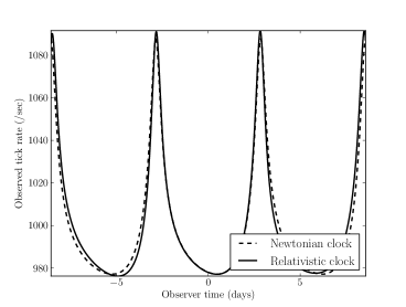
Figure 1: Illustration of the basic scenario: an observer watches a clock in a nearly Keplerian orbit around black hole, but relativity changes both the clock’s orbit, and the paths that the signals take to reach the observer. The orbits are initialised at zero proper time and then integrated forward and back, but observer time lags by about a day, because of the placement of the observer. Note how the tick rates are very similar until pericentre passage, but then the relativistic orbit appears to get ahead a little bit — that is pericentre precession. Spin effects are also included in the calculation, but too small to see at the resolution of this figure. The eccentricity of this orbit is $e=0.6$, the semi-major axis is $a=0.06\,$mpc, and the inclination $I=45^{\circ}$. For this and all other numerical results in this paper, we set the black hole mass to $20$ light seconds, cf. equation (1) .

An S star, or a pulsar on a similar orbit, can be considered as a clock in orbit around a black hole. The clock moves on a time-like geodesic and ticks at equal intervals of its proper time $\tau_{c}=n\nu_{c}$. With each tick, the clock sends out photons in all directions on null geodesics. Some of these photons reach an observer, who records their arrival times as $t_{a}(n)$. The observer can also choose to calculate the frequency by taking the derivative of the arrival times with respect to the proper time of emission:

$$\nu_{a}=\frac{1}{t_{a}(n+1)-t_{a}(n)}=\nu_{c}\left(\frac{dt_{a}}{d\tau_{e}}\right)^{-1}.$$ (2)

Figure 1 shows an example of what might be measured. For pulsars, the ticks are simply the pulses. For an S star, there are no such discrete ticks, but the clock model still applies, because

$$c\,\ln(\nu_{c}/\nu_{a})$$ (3)

has the interpretation of redshift as usually measured from spectroscopy. It is not essential for the observer to know the intrinsic frequency in advance, since $\nu_{c}$ just introduces an additive constant into equation (3). The important thing is to be able to calculate $t_{a}(n)$, for which one has to to compute time-like geodesics (orbits) and null geodesics (light paths), and solve the boundary-value problem for null geodesics from clock to observer. A moving observer can also be allowed for, if desired.

Many different relativistic effects are, in principle, measurable from a clock orbiting a black hole. First, the spacetime around the black hole dilates the clock time. Then, every term in the metric affects both the orbit of the clock and the photons from the clock, and imprints itself on the observables in its own distinctive way. The best-known examples are pericentre precession and the Shapiro time delay; the former concerns orbits while the latter influences light paths. Another difference is that precession is cumulative over many orbits, whereas the Shapiro delay is transient and does not get larger as one observes more orbits. In the solar system and for binary pulsars, both cumulative and transient effects are measurable. The circumstances of the Galactic-centre region, however, strongly favour the transients over the cumulatives for the following reasons:

1. The orbital periods are long. Cumulative build-up needs multiple orbits which takes decades.

2. Orbits of S stars tend to be highly eccentric, $e=0.9$ being typical. Relativistic effects increase more steeply with small radius and high velocity than classical effects, and hence relativity is strongest around pericentre passage.

3. The extended stellar system will contribute significant noise, hampering in particular searches which rely on build-up over long time scales. Whereas it may be possible to disentangle transient effects from noise over short time scales because the time dependence of the former is well understood.

With a full 4-dimensional relativistic treatment, this paper performs numerical experiments - computing arrival times $t_{a}$ - to gain insight into transient relativistic behaviour on S Star redshifts. Section 2 discusses the more familiar tests of the Kerr metric and discusses a few examples of transient effects, section 3.1 formalises our redshift-calculating method, and discusses how the different effects scale with orbital period. Section 3 calculates these effects for mock S Star orbits. Finally, in section 4 we propose a novel strategy based on wavelet decomposition which may help separate relativistic behaviour from Newtonian noise.

2 Familiar effects from Kerr

There are multiple relativistic effects which grow over many orbits. This has been essential to observing them in artificial satellites, planets or pulsars. Here we list some of the well-known ones.

2.1 Cumulative

1. The expected relativistic orbital precession has been discussed extensively in the context of S stars (e.g., Rubilar & Eckart, 2001; Merritt et al., 2010; Sadeghian & Will, 2011; Sabha et al., 2012) and pulsars (e.g., Liu et al., 2012). Relativity gives several contributions to the precession. The strongest cumulative relativistic effect comes from the first Schwarzschild contribution, resulting in a perihelion shift

   $$\Delta\omega=\frac{6\pi}{a(1-e^{2})}$$ (4)

   per orbit.

2. There is another contribution to the precession if the black hole has internal angular momentum. This is characterised by a spin parameter; or angular momentum per unit mass $s$. Bodies near the black hole experience frame dragging in the spin direction. The precessional effect due to this is

   $$\Delta\phi=-8\pi s\,[a(1-e^{2})]^{-3/2}$$ (5)

   per orbit. The phenomenon of frame dragging has been first observed only in recent years, by using laser ranging to accurately determine the orbit of the Lageos satellites and reveal the relativistic effect of the Earth’s spin (Ciufolini & Pavlis, 2004; Iorio, 2010). The recently launched LARES satellite aims to measure the effect to an accuracy of 1%(Ciufolini et al., 2009).

3. Two further effects act on the spin of the star or pulsar. One is geodetic precession, wherein a vector attached to an orbiting body moves by (for circular orbits)

   $$\Delta\phi=\frac{3\pi}{a}$$ (6)

   per orbit (Fließbach, 1990). Gravity Probe B has measured this effect in Earth’s gravitational field (Everitt et al., 2011). The parallel transport of a vector along a geodesic is also influenced by frame-dragging. This is called the Lens-Thirring effect, and was also detected by Gravity Probe B (Everitt et al., 2011). It is possible that the spin axis of a close-in pulsar be parallel transported enough to change the pulse profile. Pulse-profile changes from geodetic precession have been observed in Binary Pulsar systems (Kramer, 1998; Weisberg & Taylor, 2002; Breton et al., 2008; Hotan, Bailes & Ord, 2005), and could be observed in galactic centre pulsars.

   Orbital decay due to gravitational radiation is another well-known effect, but the time scales are too slow to be interesting for Galactic-centre stars.

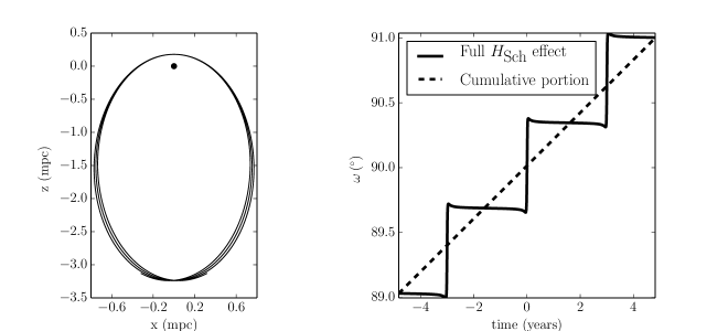
Figure 2: Illustration of Schwarzschild precession. The orbit is like a 1/3-size version of the star S2 (Gillessen et al., 2009a), with semi-major axis $a=0.041^{\prime\prime}$ and eccentricity $e=0.88$, but viewed face-on. We have set the distance to the galactic centre at $8.31\,$kpc. Along the trajectory we may associate a value for the argument of pericentre $\omega$ to the value it would take were the phase space position a solution to Kepler’s equations. The right panel shows the instantaneous argument of pericentre against coordinate time for a distant observer. We see here that, for high eccentricities, precession is concentrated so strongly around pericentre that it looks nearly discrete. The dashed curve is the well-known formula (4) for the cumulative precession.

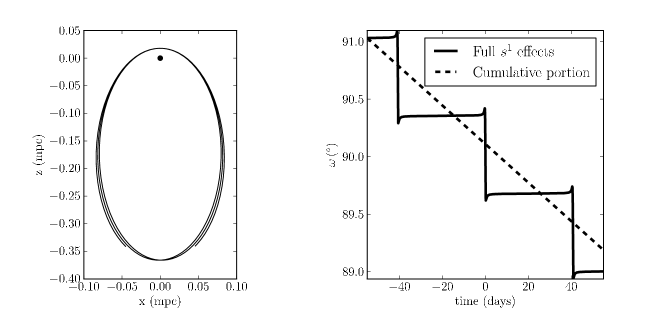
Figure 3: Illustration of frame-dragging precession. Since the effect is higher order than Schwarzschild precession, a smaller orbit is used than in Figure 2 in order to make the precession visible: the orbit is a 1/30-sized version of the star S2 (here with $e=0.88$ and $a=0.0041^{\prime\prime}$), yet viewed face-on. The spin is maximal and perpendicular to the orbit; were the spin direction not perpendicular to the orbital plane, the orbital plane would also precess about the spin axis. Frame-dragging is even more strongly concentrated around pericentre than Schwarzschild precession. The dashed curve is the formula (5).

2.2 Transients

Unlike the orbits of satellites, planets or pulsars, in the Galactic centre, orbital periods are much longer, so accumulating relativistic signals over many orbits is difficult even though the fields are far stronger. Perhaps an even more serious problem is the Newtonian perturbations due to gas and other stars in the Galactic-centre region. So it is interesting to think about transient effects which occur over a single orbit. These may be measurable over a short time, and moreover a predictable time dependence could enable extracting the signal from the Newtonian background. In fact, there is a plethora of such effects, a few of which we describe here.

1. The strongest relativistic effect is gravitational time dilation, one of the basic consequences of the Equivalence Principle. Time is dilated by a factor

   $$g_{tt}^{-1/2}=1-\frac{2}{r}$$ (7)

   with no effect at this order on the orbit or the light paths. For a highly eccentric orbit, clearly there will be a peak at pericentre. GNSS satellites are sensitive to this shift. For navigation demands, it is enough for GNSS satellites to routinely step the on-board clock time back, correcting for this effect. Gravitational time dilation has not yet been measured in the galactic centre, but is expected to be possible in the near future (Zucker et al., 2006). If observed, gravitational time dilation would provide a new test of the Einstein Equivalence Principle (Angélil & Saha, 2011).

2. Lensing effects of gravity on photons travelling to us are naturally also transient phenomena. Astrometric shifts due to gravitational lensing have been discussed in the Galactic-centre context (Bozza & Mancini, 2009), as have time delays due to a curved space-time (Angélil & Saha, 2010), although none have yet been detected. With an impact parameter $b$, the deflection angle of a null ray is

   $$\Delta\phi=\frac{4}{b}.$$ (8)

   This is the leading-order Schwarzschild contribution. The $\sim b^{-2}$ effect is also relevant, and enters at the same order as the frame-dragging lensing contribution, which we discuss later. The extra delay induced in the arrival time of a packet of light compared to had it travelled in a straight line is the Shapiro delay (Shapiro, 1964), and has been well-tested with the Mariner 9 and Viking spacecraft in the solar system(Shapiro et al., 1968, 1977; Reasenberg et al., 1979) and in binary pulsar systems(Stairs, 2003; Demorest et al., 2010).

3. Underlying every type of orbit precession, there is a fleeting contribution which occurs around pericentre, the memory of which is not retained by the orbit’s shape afterwards. Figure 2, which we shall return to later, shows our first example: the precession of the instantaneous pericentre of a highly eccentric orbit. Far from being the smooth effect suggested by equation (4), it consists almost of discrete kicks. In the derivation of (4), an oscillatory term crops up beside this term. Because this term imparts a momentary perturbation which time-averages to zero, it is dropped in textbook derivations.(Weinberg, 1972; Misner, Thorne & Wheeler, 1973; Schutz, 2009; Carroll, 2004). Analogously, Figure 3 shows pericentre precession due to frame dragging by the black hole spin, of which (5) is the average. These two examples are artificial and do not themselves correspond to observable quantities, for two reasons. First, for Figure 3, we have dropped lower-order contributions from space curvature so as to isolate frame dragging. Second, the instantaneous pericentre of an orbit is defined as the pericentre of a Keplerian orbit with the same instantaneous position and momentum (the osculating elements, see e.g. Murray & Dermott, 1999). In relativity, the instantaneous pericentre therefore becomes gauge-dependent and hence is not an observable quantity (cf. Preto & Saha, 2009). Nonetheless Figures 2 and 3 do suggest that time-resolved observations could detect relativistic effects over a single orbit, especially around pericentre, where relativity is strongest and Newtonian perturbations are likely to be at their weakest.

In Section 3 below, we show how these and several other effects can be readily calculated numerically using a Hamiltonian formalism, and show various illustrative examples.

3 Time delays and redshifts in Kerr

3.1 The Hamiltonian

The Hamilton equations for

$$H={\textstyle\frac{1}{2}}\,g^{\mu\nu}\,p_{\mu}\,p_{\nu}\,,$$ (9)

are simply the geodesic equations, with the affine parameter taking on the role of the independent variable. Since $H$ does not depend explicitly on the affine parameter, $H$ is constant along a geodesic. Proper time is $\sqrt{|H|}$ times the affine parameter, except for the case of $H=0$, corresponding to null geodesics.

Table 1: Hamiltonian terms for orbits and light paths in a Kerr spacetime. The full Hamiltonian (9) is the sum of all the terms in the left column, plus higher-order terms that we have not considered. The middle and right terms group the terms by physical effect and scaling of the time delay $\Delta t$ with period $P$, as explained in Section 3.1 Note that we are using geometrised units $GM=c=1$ here. To put $\Delta t$ and $P$ in time units, simply multiply by a power of $GM/c^{3}$ so as to get the dimensions right.

		Orbits	Light paths
	$\displaystyle\vrule width=0.0pt,height=24.0pt,depth=20.0pt-\frac{p_{t}^{2}}{2}$	static	—Rømer $\Delta t\sim P^{\,2/3}$
	+$\displaystyle\vrule width=0.0pt,height=24.0pt,depth=20.0pt\frac{\bf{p}^{2}}{2}$	—Kepler $\Delta t\sim P^{\,2/3}$
	$\displaystyle\vrule width=0.0pt,height=24.0pt,depth=20.0pt-\frac{p_{t}^{2}}{r}$		—Shapiro $\Delta t\sim P^{\,0}$
	$\displaystyle\vrule width=0.0pt,height=24.0pt,depth=20.0pt-\frac{(\bf{x}\cdot\bf{p})^{2}}{r^{3}}$	—Schwarzschild $\Delta t\sim P^{\,0}$
	$\displaystyle\vrule width=0.0pt,height=24.0pt,depth=20.0pt-\frac{2p_{t}^{2}}{r^{2}}$
	$\displaystyle\vrule width=0.0pt,height=24.0pt,depth=20.0pt-\frac{2p_{t}\bf{p}\cdot\left(\bf{s}\times{x}\right)}{r^{3}}$	—frame-dragging $\Delta t\sim P^{\,-1/3}$	—frame-dragging, spin-squared, Shapiro $\Delta t\sim P^{\,-2/3}$
	$\displaystyle\vrule width=0.0pt,height=24.0pt,depth=20.0pt+\frac{s_{\perp}^{2}}{2r^{4}}\left(\bf{x}\cdot\bf{p}\right)^{2}-\frac{1}{2r^{4}}\frac{\left(\bf{p}\cdot\bf{s}\times\bf{x}\right)^{2}}{s_{\perp}^{2}}$
	$\displaystyle\vrule width=0.0pt,height=24.0pt,depth=20.0pt-\frac{1}{2r^{4}}\frac{1-s_{\perp}^{2}}{1-s_{\parallel}^{2}}\left(\left(\bf{p}\cdot\bf{s}\right)r-\frac{\left(\bf{x}\cdot\bf{s}\right)\left(\bf{x}\cdot\bf{p}\right)}{r}\right)^{2}$	—Spin (even), Schwarzschild $\Delta t\sim P^{\,-2/3}$
	$\displaystyle\vrule width=0.0pt,height=24.0pt,depth=20.0pt+\frac{p_{t}^{2}}{r^{3}}s_{\perp}^{2}-\frac{4p_{t}^{2}}{r^{3}}$		not included

In our case, $g^{\mu\nu}$ are the contravariant components of the Kerr metric. The Kerr metric is a vacuum solution to the Einstein Field Equations. This is the appropriate metric to use if we are interested in solving the forward problem for relativistic effects. This will allow us to investigate examples of transient relativistic effects in isolation. In section 4 we treat the more realistic case; we relax the vacuum assumption, and add other S stars as Newtonian perturbers to the system, and see whether we can uncover transient relativistic effects when the Newtonian noise is significantly large.

Assuming the orbits and light paths do not go close to the horizon, we can expand the Hamiltonian in powers of $1/r$. The result is available in Angélil & Saha (2010). However because it is convenient to be able to set the black hole spin direction without having to rotate the observer and the orbit, we use a slightly different form. The Kerr geometry in Boyer-Lindquist coordinates necessarily aligns the axis of symmetry of the coordinate system with the axis of symmetry of the space-time geometry itself, and it is therefore not possible to disentangle the preferred direction of the coordinates with that of the spin in these coordinates. This means we need to first transform to pseudo-Cartesian coordinates. Table 1 contains the form of the Hamiltonian which we use here, in pseudo-Cartesian coordinates, and with the spin promoted to a 3-vector $\mathbf{s}=\left(s_{x},s_{y},s_{z}\right)$. (An equivalent table is given in Angélil et al., 2014, but using Boyer-Lindquist variables.) For convenience, we use the short-form

$$s_{\perp}\equiv\frac{\bf{s}\times\bf{x}}{r}\qquad\textrm{and}\qquad s_{\parallel}\equiv\frac{\bf{s}\cdot\bf{p}}{r}.$$ (10)

Presenting the Hamiltonian in table form allows us to group the terms according to physical effects on orbits or light paths. The Kepler/Rømer terms are classical. The leading relativistic effect is time dilation, but as it is not associated with geodesics as such, it does not appear in the table. Relativistic terms not depending on the spin parameter $s$ are labelled ‘Schwarzschild’. Then there are various terms depending on spin. Of these, the term odd in $s$ gives frame dragging.

We are now ready to use the Hamilton equations corresponding to the Hamiltonian in table 1 to explore the dynamics, and the consequences of the many terms in Table 1. While Angélil, Saha & Merritt (2010) solves the inverse problem for relativity on S stars, here we attempt to give a more qualitative picture of exactly how relativity perturbs the orbit and redshifts/arrival-times, in particular for transient effects.

3.2 Numerical Experiments with S Stars and Pulsars

We have already referred to Figure 1, in passing in the Introduction. That figure compares the observable pulse rate from two cases: (i) a clock follows a relativistic orbit and the ticks are conveyed to the observer along null geodesics, and (ii) the classical case including Kepler and Rømer effects, and time dilation. The relativistic case includes all terms in Table 1, other than the two highest-order “not included” terms in the light path. The orbits are initialised at apocentre with $e=0.6$ and inclination $I=45^{\circ}$ with respect to the line of sight, and are integrated forward and back. The rest-frame tick rate of the clock is 1000 Hz and its orbital period is a week, while the assumed gravitational radius of the black hole is $GM/c^{2}=20\,\hbox{light-sec}$ (corresponding to Sgr A*) — these choices are only for the sake of putting axes on the figure and have no physical significance.

From Figure 1 we can infer that relativity makes the pericentre precess, but to see more detail we need to extract the difference between the relativistic and non-relativistic cases. It is especially interesting to see what different groups of terms from Table 1 do to the time-delay and redshift curves. To label different cases, let us introduce some shorthand, as follows.

1. $H_{\rm sch}$ means that Schwarzschild terms but not spin terms have been included in the orbits, while no relativistic terms have been included for the light paths. These are the forth and fifth rows in Table 1. $H^{\rm sch}$ means that Shapiro terms have been included for the light paths, while the orbits are classical. These are the third and fourth rows in Table 1.

2. $H_{s}$ ($H^{s}$) means that only the spin $p_{t}\left(\mathbf{x}\times\mathbf{p}\right)/{r^{3}}$ term has been added to the classical terms, and only for orbits (light paths). This term is found in the sixth row in Table 1.

3. Similarly, $H_{s^{2}}$ ($H^{s^{2}}$) means classical plus spin-squared terms in the orbits (light paths). These terms are the remaining rows of Table 1.

Figures 2 and 3, mentioned in the previous section, show the orbit effects $H_{\rm sch}$ and $H_{s}$ as a perturbation to pure Newtonian motion. Cumulative precession is a discrete phenomenon which occurs at pericentre. However, the effect is not completely step-like, with transient behaviour before and after the pericentre kicks. The complicated $H_{s^{2}}$ orbit evolution effects are shown in Figure 4. The evolution depends on the relative orientation of the orbital angular momentum with the black hole spin. We do not have any interpretation that helps understand the dynamics generated by these higher-order terms, and merely show this orbit as an example.

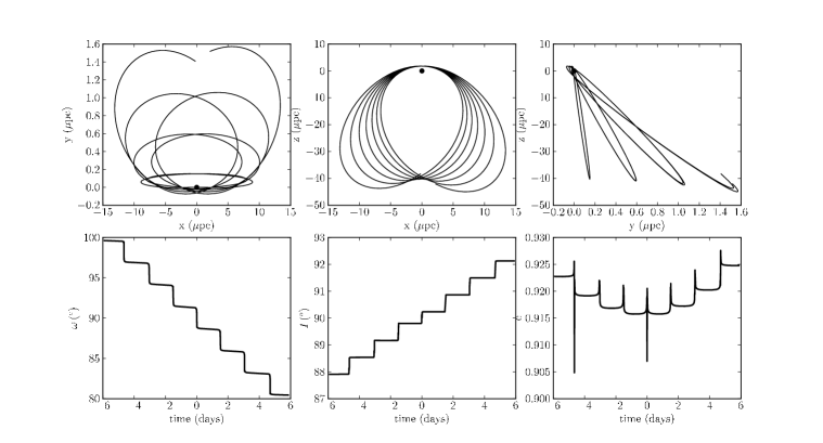
Figure 4: Orbital effects of $H_{s^{2}}$ (even-spin terms). The orbit is like a 1/300-size version of S2 ($a=0.02\,$mpc and $e=0.88$), initially in the $x$-$z$ plane, while the spin is along $x$. Schwarzschild and frame-dragging terms have been omitted, so this is a completely artificial example. It is nonetheless interesting, as it illustrates the complexity of the spin-derived effects, from which none of the Keplerian orbital elements are exempt from change.

Moving now to light-path effects, Figure 5 shows the contribution of $H^{\rm sch}$, and Figure 6 shows the contributions of $H^{s}$ and $H^{s^{2}}$. The even-spin signals on timing and redshift are capable of a wide variety of signal shapes, which depend on the orbit geometry relative to the observer and the spin-direction. Timing delays due to spin effects influencing photon paths have been calculated for binary pulsars (see for example Fig. 5 in Wex & Kopeikin, 1999).

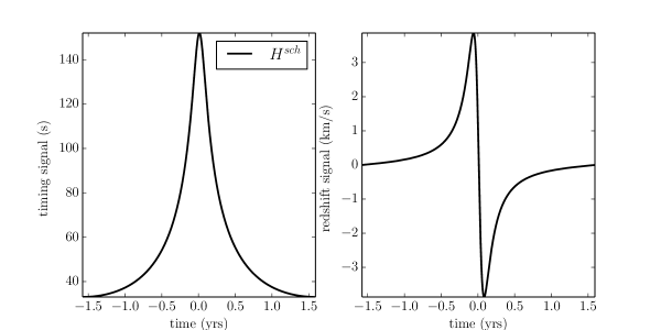
Figure 5: Light-path contributions to time delays and redshifts of Schwarzschild terms. The left panel is simply the well-known Shapiro delay. The redshift is the derivative of the time-delay, stated in eq. (2). The orbital period is $3\,$yrs - a scaled version of the orbits used for Fig.  1: $e=0.6$, $a=0.041^{\prime\prime}$, $I=45^{\circ}$, and $R_{0}=8.31\,$kpc. The time delay depends only logarithmically on the period $P$, but the redshift signal scales as $1/P$. Because this is a light-propagation effect, there is no cumulative component to this effect.

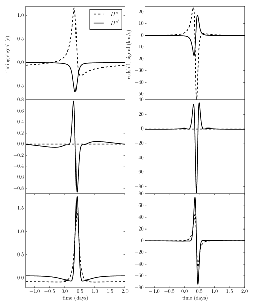
Figure 6: Light-path contributions of spin terms to time delays and redshifts. The orbit in each case is 1/50-sized version of the one in Figure 5 ($a=0.0008^{\prime\prime}$, $e=0.6$), while the spin is maximal. Only the spin direction changes: in the top row, the spin is perpendicular to the orbit; in the middle row, the spin is along the line of sight, and hence the frame-dragging signal is null, leaving only even-spin contributions; in the bottom row, the spin is perpendicular to the line of sight.

3.3 Scaling

Table 1 also gives the scaling of the time delay, which depends on some power of the orbital period $P$. For the classical Kepler or Rømer effect $\Delta t\sim P^{2/3}$. With respect to the relevant terms in the Hamiltonian, we thus have

$$\mathbf{p}^{2}\;\Rightarrow\;\Delta t\sim P^{2/3}\,.$$ (11)

The $p_{t}^{2}/r$ behaves differently for orbits and light paths. For orbits, it is of course part of Keplerian dynamics. For light paths it is part of the Shapiro delay, which depends only logarithmically on $r$. Accordingly, we write

$$\frac{p_{t}^{2}}{r}\;\Rightarrow\;\Delta t\sim\begin{cases}P^{2/3}&\mbox{orbits}\\ P^{0}&\mbox{light paths}.\end{cases}$$ (12)

Table 1 also has many terms which look like increasingly elaborate versions of the classical ones. The scaling of $\Delta t$ for such terms is simple: provided we are not close to the horizon, a factor of $1/r$ in a Hamiltonian term introduces a factor $P^{-2/3}$ in the time delay. That leaves only the $p_{t}\,\bf{x}\times\bf{p}$ term to deal with. To do that, we consider the geometric mean of $\mathbf{p}^{2}$ and $p_{t}^{2}/r^{4}$ to get

$$\frac{p_{t}\bf{x}\times\bf{p}}{r^{3}}\;\Rightarrow\;\Delta t\sim\begin{cases}P^{-1/3}&\mbox{orbits}\\ P^{-2/3}&\mbox{light paths}.\end{cases}$$ (13)

Table 1 includes all terms with $\Delta t$ contributions up to $P^{-2/3}$.

Redshifts scale like

$$\frac{\Delta t}{P}$$ (14)

as will be evident from Equations (2) and (3). This assumes, as before, that orbits and light paths are not too close to the horizon. This suggests that prospects for testing relativity as period sizes decrease improve quicker for stellar orbits than pulsar orbits.

We can test these scalings with numerical experiments. In Figure 7, we show how the transient-relativistic contribution of $H_{\rm sch}$, $H_{s}$ and $H_{s^{2}}$ scale with the orbital period $P$. We isolate the transient signal by calculating the most-positive plus most-negative difference in the observables, upon initialising two orbits at pericentre integrating over one period with and without the Hamiltonian terms in question. All orbits have $e=0.6,I=45^{\circ}$, as in Figure 1, but the period was varied. As we can see in the figure, the predicted scalings from Table 1 are borne out. Note, in particular, that the leading-order Schwarzschild effects on the orbit makes for timing signals which remain constant as the orbital size deceases. The redshift contribution of Schwarzschild however, scales as $1/P$. Figure 8 then shows how the light-path contributions scale with period. For the latter figure, the spin is maximal and perpendicular to the orbit, but this detail is unimportant for the scaling.

For both orbit and light-path effects, our simulations show that

1. the relativistic contributions are concentrated around pericentre, and

2. vary along the orbit in a complicated way, (especially when spin is included), yet

3. nonetheless agree with the orbital period scalings in Table 1.

As we shall see in the next section, (i) and (iii) will prove useful for extracting relativistic signals from extended mass noise.

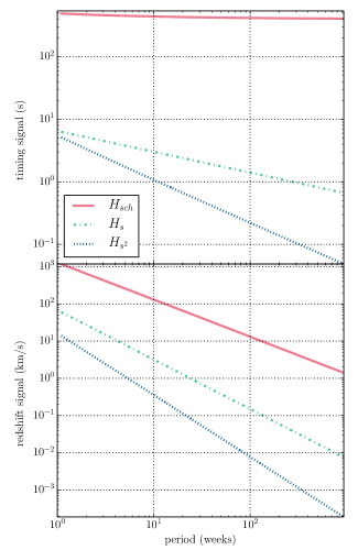
Figure 7: Transient orbital contributions to time delays and redshifts of different relativistic terms (Schwarzschild, frame-dragging and spin-squared), as a function of orbital period. The cumulative components of these relativistic effects have significantly smaller amplitude. The orbit size used in Figure 1 corresponds to the short-period end of these panels. The orbital geometry we maintain over this calculation has $I=45^{\circ}$, and $e=0.6$.

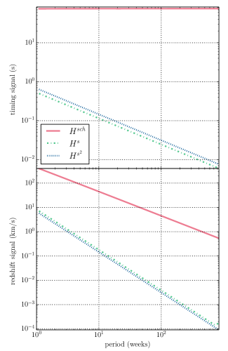
Figure 8: Light-path contributions to time delays and redshifts of different relativistic terms. This figure complements Figure 7. The main difference is in how the odd-spin (or frame-dragging) term scales.

4 Filtering Newtonian perturbations

Orbit fitting in the pure Kerr case poses no fundamental problems (Angélil, Saha & Merritt, 2010), however, critical to being able to resolve relativistic effects on galactic centre stars will be the handling of other perturbations. The most significant are expected to be those from the extended mass distribution, mainly from other stars, but also perhaps from a significant dark matter component. Merritt et al. (2010), Antonini & Merritt (2013) and Iorio (2011) compare the cumulative effects of extended mass and relativity.

In this section we are interested in transient relativistic signals over a single orbit. A star whose redshift/time-delay is expected to be influenced by relativity is the target star. The redshift/time-delay of this star is also affected by the Newtonian attraction of other black hole-orbiting stars in the neighbourhood, which we call the perturbers.

While the relativistic time dilation signal is likely to be stronger than extended Newtonian signals, the next-strongest effects (Schwarzschild and Shapiro) may be partially obscured. In this section we first discuss how to calculate the Newtonian perturbations on the target star, before introducing a wavelet decomposition method as a tool which could be used to help distinguish them from relativistic perturbations.

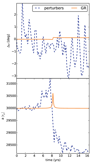
Figure 9: The evolution of the instantaneous Keplerian elements $a$ and $\omega$. The Newtonian perturbations from other stars are distributed throughout the orbit, whereas relativistic perturbations are concentrated near pericentre. (Note that the instantaneous $a$ and $\omega$ are not directly observable in relativity, because they are gauge-dependent and don’t take signal propagation into account. The observable quantities are arrival times and redshifts.)

4.1 Newtonian perturbers

The classical leading-order perturbation due to other stars orbiting the black hole is given by a Hamiltonian contribution

$$H_{\textrm{stellar}}=\sum_{j}\frac{m_{j}}{M}\left(\frac{{\vec{x}}\cdot{\vec{x}}_{j}}{|{\vec{x}}_{j}|^{3}}-\frac{1}{|{\vec{x}}-{\vec{x}}_{j}|}\right),$$ (15)

where ${\vec{x}}$ is the star being observed and $m_{j},{\vec{x}}_{j}$ refer to perturbing stars. For a derivation, see Wisdom & Holman (1991), especially their equation (17), and disregard the mutual perturbations of the ${\vec{x}}_{j}$ stars. Note however, that the back-reaction on the observed star due to the perturbed position of the black hole must be included. We model the perturbations by adding the classical perturbation (15) to the relativistic Hamiltonian from Table 1. Will (2014) shows that new relativistic terms appear in general $N$-body problems, if there is a tidal force or a quadrupole of the same order as the dominant monopole. If the star being observed were in a binary, such terms would arise, but for the simpler problem we are considering, the approximation of simply adding the classical perturbers appears to be valid.

As an example of the effect of Newtonian perturbers, we consider a target star at $\vec{x}$ on an S2-like orbit (Gillessen et al., 2009b) with semi-major axis $a=30000$ in geometric units, and eccentricity $e=0.9$. The perturbers at ${\vec{x}}_{j}$ are 100 stars, all of equal mass, together making up $1\%$ of the black hole’s mass or $\simeq 4\times 10^{4}M_{\odot}$. These are distributed according to a power-law profile $\rho\left(r\right)\propto\exp\left({-\gamma r}\right)$ with $\gamma=0.5$. Their eccentricity distribution is uniform. Figure 9 contrasts the Newtonian and relativistic perturbations on the target star’s semi-major axis $a$ and periapsis argument $\omega$. As we see, the relativistic perturbations are completely submerged under the Newtonian stellar perturbations. We may recall that for Mercury, Newtonian perturbations from other masses are an order of magnitude larger than the relativistic effects, yet the accumulation of $\Delta\omega\simeq 0.1^{\prime\prime}$ per orbit is measurable. What makes such a measurement possible is that in the solar system, planetary masses are known accurately and hence the Newtonian perturbations can be subtracted off. Near the Galactic Centre, there is no prospect of measuring all the perturbing masses accurately. Hence, if the model perturbers in Figure 9 are at all representative, relativistic effects would be drowned under Newtonian perturbations.

4.2 Wavelets

However, the situation is not hopeless. Because the transient relativistic effects have a very specific time dependence that is known in advance, it may be possible to extract them from under the Newtonian background. Matched-filter techniques, well known from gravitational-wave searches (see for example Sathyaprakash & Schutz, 2009), will not work because the observables are non-linear in the perturbing effects. But progress may be possible using wavelets.

Table 2: The coefficient structure of a wavelet-transformation. The first index gives the time scale, the second index give the localisation.

$n$	$C_{n,m}$
$0$	$C_{0,1}$
$1$	$C_{1,1}$
$2$	$C_{2,1},C_{2,2}$
$3$	$C_{3,1},C_{3,2},C_{3,3},C_{3,4}$
$4$	$C_{4,1},\hskip 14.22636pt\ldots\hskip 14.22636pt,C_{4,8}$
$5$	$C_{5,1},\hskip 14.22636pt\ldots\hskip 14.22636pt,C_{5,16}$

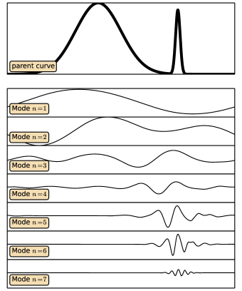
Figure 10: In this demonstration, a sum of two Gaussians (top panel) is decomposed into the Daubechies 20 wavelet basis (other panels). Each of the wavelet panels corresponds to (17) for the stated value of $n$. (The constant $0$-th mode is not shown.) The sum of the lower panel curves yields the parent shape.

A wavelet decomposition (Daubechies, 1988, 1990), allows one to identify features by breaking down a signal according not just to the frequency at which they occur, but also according to the time they occur. In contrast to a Fourier decomposition, where each basis function carries frequency information only, a wavelet basis function includes both frequency and localisation information. Relativistic perturbations and perturbations due to the extended mass affect the dynamics in different ways, as Figure 9 illustrates, at different frequencies and different localisations. We are interested in designing a procedure which helps identify relativistic signals when shrouded by significant extended-mass noise. Because redshift curves over a single orbit have no periodicity, and because relativistic perturbations are most prevalent around pericentre, wavelets are a natural choice for designing filters. As a result of relativistic effects being most pronounced around pericentre — and non-lingering due to their oft transient nature — we can expect high-frequency coefficients, localized around pericentre passage, to be of greatest value in retaining information from relativistic effects. We would expect the extended mass perturbations to also impart transient, high-frequency effects, such as close encounters, but those would not be concentrated around pericentre.

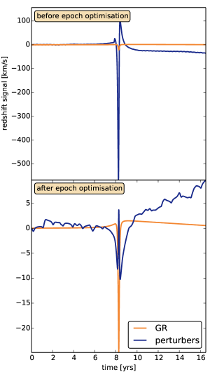
Figure 11: The upper panel shows the pure signals $z_{\textrm{GR}}-z_{\textrm{Kepl}}$ and $z_{\textrm{Pert}}-z_{\textrm{Kepl}}.$ In our chosen example, the perturbation from the extended mass distribution is $\sim 30$ times larger than the relativistic signal. The lower panel shows the signals after shifting epochs to minimise the area under the curves. It is the latter we plug into the wavelet procedure detailed in section 4.

In a typical wavelet decomposition, such as the Daubechies 4 and Daubechies 20 wavelet types, a signal is expressed as

$$z(t)=\sum_{n}\sum_{i=1}^{2^{n}}C_{ni}\psi_{ni}(t).$$ (16)

The wavelet basis functions $\psi_{ni}(t)$ are the scaled and translated versions of a single function, called the mother wavelet, while the $C_{ni}$ are the expansion coefficients. Table 2 schematically outlines the wavelet coefficient structure. Each row of this table corresponds to a particular time scale, which is twice as fast as in the row above it. The $n$-th row has $2^{n}$ coefficients, each of which correspond to different time windows (or localisations). Let us write

$$\mathcal{W}_{n}\,z(t)\equiv\sum_{i=1}^{2^{n}}C_{ni}\psi_{ni}(t).$$ (17)

The operator $\mathcal{W}_{n}$ isolates a particular time scale in the signal.

Figure 10 shows the result of applying the $\mathcal{W}_{n}$ operator to an example curve, consisting of two superposed Gaussians with different means and widths. We see that $n=2$ the first (wider) Gaussian dominates, at $n=3$ the second Gaussian starts to take over, and from $n=5$ the first Gaussian has been completely filtered out and only the narrower Gaussian contributes.

4.3 Filtering relativistic signals with wavelets

We now consider an S star (or S pulsar) whose redshift (or pulse arrival times) are contaminated by significant noise from an extended mass system, and investigate how the wavelet coefficients are influenced by relativistic versus extended-mass perturbations. Starting with an unperturbed Keplerian orbit, we proceed as follows.

First, we generate three redshift curves for this orbit: $z_{\textrm{Kepl}}$ has no perturbations, $z_{\textrm{Pert}}$ includes the Newtonian perturbation by including the effects of (15), and $z_{\textrm{GR}}$ includes only the relativistic Schwarzschild and Shapiro perturbations. The differences $z_{\textrm{GR}}-z_{\textrm{Kepl}}$ and $z_{\textrm{Pert}}-z_{\textrm{Kepl}}$ are plotted in the upper panel of Figure 11. Here we use the same extended Newtonian mass system example as earlier in this section, corresponding to Figure 9. In this mock data example, the relativistic redshift signal is $\sim 30$ times weaker than that due to the extended mass perturbations.

Before taking wavelet transforms, another step is necessary: we need to choose the reference orbit $z_{\textrm{Kepl}}$ anew, because of course the “original” unperturbed orbit will not be provided by data. It would be natural to choose a reference orbit that best fits the data, but any consistent convention can be used. For simplicity, we shift the epoch of $z_{\textrm{Kepl}}$ so as to minimize the integrated difference from $z_{\textrm{GR}}$ and $z_{\textrm{Pert}}$ respectively. We denote the shifted Keplerian curves as $\tilde{z}_{\textrm{Kepl}}$ and $\bar{z}_{\textrm{Kepl}}$. The differences $z_{\textrm{GR}}-\tilde{z}_{\textrm{Kepl}}$ and $z_{\textrm{Pert}}-\bar{z}_{\textrm{Kepl}}$ are plotted in Figure 11’s second panel. In this example, they have approximately the same amplitude.

We then decompose the signals into different modes according to frequencies and plot the differences

$$\mathcal{W}_{n}\,\left(z_{\textrm{GR}}-\tilde{z}_{\textrm{Kepl}}\right)$$ (18)

and

$$\mathcal{W}_{n}\,\left(z_{\textrm{Pert}}-\bar{z}_{\textrm{Kepl}}\right)$$ (19)

for $n=1\ldots 9$. These are plotted in Figure (12), which shows the results using two different wavelet basis functions.

In our example, the wavelet-reconstructed perturber signal is stronger than the relativistic ones over all wavelet scales, except at $n=5$ (with twice the amplitude) and $n=6$ (with almost the same amplitude). This decomposition procedure indicates that given the geometry of our chosen orbit, Schwarzschild effects, although obscured by extended mass perturbations with a signal-to-noise $S/N\sim 1/30$, will impart a significant contribution on the $n=6$ frequency modes. Alternatively, one can say that Schwarzschild effects, though about 30-fold weaker overall than extended-mass perturbations (in this model), nonetheless stand out over Newtonian perturbations over a two-year interval around pericentre, in wavelet modes of timescale $\approx 6$ months.

The above suggests that subtracting off a Keplerian orbit, applying a wavelet transform to the residual, and then considering a specific subset of the wavelet coefficients may succeed in filtering out Newtonian perturbations.

5 Conclusions and Outlook

Galactic centre stars travel upon the most relativistic orbits known. However, the accessible relativistic effects are not simply extensions of similar experiments in the solar system and in binary pulsars. S stars, and S pulsars if they exist, live in stronger fields than binary pulsars, but their orbital periods are much longer. The combination of the strong fields, long orbital time-scales, and the typically high eccentricities push otherwise negligible aspects of dynamics near a black hole into the observables. For example, precession is not a steady process, as the well-known orbit-averaged formulas (4) and (5) may suggest, but nearly a shock that happens at pericentre. The concentration of dynamical effects around pericentre passage applies even more to effects which depend on the spin of the black hole. These pericentre shocks will be important when separating relativistic signals from noise sources.

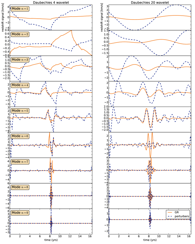
Figure 12: Reconstructed signals from wavelet frequency modes. Due to the linearity of the wavelet transformation, the sum of the signals in each column yield the lower panel curves of figure 11. The wavelets down the left column are the Daubechies 4 variety, and those down the right the Daubechies 20. Despite the raw relativistic signal being 30 times less than that from Newtonian effects due to the perturbing stars, the relativistic signal manages to significantly dominate at $n=6$. This happens for both wavelet types used here, Daubechies 4 and Daubechies 20. This procedure highlights the specific time and frequency localisation properties of the two effect types, and tools like this could aid future searches in decorrelating them.

If the observed dynamics is found to be in agreement with a Kerr space-time plus perturbations from the surrounding astrophysical environment, Einstein gravity will be tested to a new level. A further benefit is that because we test gravity by tracking freely-falling bodies, as well as photon paths, by inferring the components of the metric by looking at their effects on the behaviour of geodesics, we probe not just the field equations, but implicitly test the notion requisite to describing gravity with geometry - the principle of equivalence.

The spectrometers of the Keck and VLT telescopes have independently observed the spectra of the S stars, managing to achieve spectral resolution to $\sim 10\rm\,km\,s^{-1}$ in the best cases. The next generation of instruments, such as the High Resolution Near-infrared Spectrograph (SIMPLE) on the E-ELT is expected to achieve $\sim 2\rm\,km\,s^{-1}$ (Origlia, Olivia & Maiolino, 2010). If an S star with period $\sim 1$ year is discovered, observations clustered around pericentre passage at this level of accuracy could provide a measurement for frame-dragging. Were S pulsars with stable periods to be detected with orbits similar to the already-known S stars, pulsar timing even at the msec level would be, in principle, enough for all the effects summarised in Table 1. The challenge would be removing the Newtonian “foreground” due to the extended mass distribution around Sgr A*. Separating cumulative effects into Newtonian versus relativistic is a challenging task, yet with transient effects that vary along an orbit in different ways, one can be more optimistic.

References

- Angélil & Saha (2010) Angélil R., Saha P., 2010, The Astrophysical Journal, 711, 157
- Angélil & Saha (2011) Angélil R., Saha P., 2011, The Astrophysical Journal Letters, 734, L19
- Angélil et al. (2014) Angélil R., Saha P., Bondarescu R., Jetzer P., Schärer A., Lundgren A., 2014, Physical review D
- Angélil, Saha & Merritt (2010) Angélil R., Saha P., Merritt D., 2010, The Astrophysical Journal, 720, 1303
- Antonini & Merritt (2013) Antonini F., Merritt D., 2013, Astrophysical Journal Letters, 763, L10
- Ashby (2003) Ashby N., 2003, Living Reviews in Relativity, 6, 1
- Bozza & Mancini (2009) Bozza V., Mancini L., 2009, Astrophysical Journal, 696, 701
- Breton et al. (2008) Breton R. P. et al., 2008, Science, 321, 104
- Broderick et al. (2014) Broderick A. E., Johannsen T., Loeb A., Psaltis D., 2014, ApJ, 784, 7
- Carroll (2004) Carroll S. M., 2004, Spacetime and geometry. An introduction to general relativity
- Ciufolini et al. (2009) Ciufolini I., Paolozzi A., Pavlis E. C., Ries J. C., Koenig R., Matzner R. A., Sindoni G., Neumayer H., 2009, Space Science Reviews, 148, 71
- Ciufolini & Pavlis (2004) Ciufolini I., Pavlis E. C., 2004, Nature, 431, 958
- Cordes & Lazio (1997) Cordes J. M., Lazio T. J. W., 1997, The Astrophysical Journal, 475, 557
- Daubechies (1988) Daubechies I., 1988, Information Theory, IEEE Transactions on, 34, 605
- Daubechies (1990) Daubechies I., 1990, Information Theory, IEEE Transactions on, 36, 961
- Demorest et al. (2010) Demorest P. B., Pennucci T., Ransom S. M., Roberts M. S. E., Hessels J. W. T., 2010, Nature, 467, 1081
- Doeleman (2010) Doeleman S., 2010, in 10th European VLBI Network Symposium and EVN Users Meeting: VLBI and the New Generation of Radio Arrays
- Eckart et al. (2005) Eckart A., Schödel R., Moultaka J., Straubmeier C., Viehmann T., Pfalzner S., Pott J.-U., 2005, in American Institute of Physics Conference Series, Vol. 783, The Evolution of Starbursts, S. Hüttmeister, E. Manthey, D. Bomans, & K. Weis, ed., pp. 17–25
- Eisenhauer et al. (2003) Eisenhauer F., Schödel R., Genzel R., Ott T., Tecza M., Abuter R., Eckart A., Alexander T., 2003, Astrophysical Journal Letters, 597, L121
- Everitt et al. (2011) Everitt C. W. F. et al., 2011, Physical Review Letters, 106, 221101
- Fließbach (1990) Fließbach T., 1990, Allgemeine Relativitätstheorie., Fließbach, T., ed.
- Ghez et al. (2008) Ghez A. M. et al., 2008, The Astrophysical Journal, 689, 1044
- Gillessen et al. (2009a) Gillessen S., Eisenhauer F., Fritz T. K., Bartko H., Dodds-Eden K., Pfuhl O., Ott T., Genzel R., 2009a, Astrophysical Journal Letters, 707, L114
- Gillessen et al. (2009b) Gillessen S., Eisenhauer F., Trippe S., Alexander T., Genzel R., Martins F., Ott T., 2009b, The Astrophysical Journal, 692, 1075
- Hotan, Bailes & Ord (2005) Hotan A. W., Bailes M., Ord S. M., 2005, The Astrophysical Journal, 624, 906
- Iorio (2010) Iorio L., 2010, Central European Journal of Physics, 8, 25, 10.2478/s11534-009-0060-6
- Iorio (2011) Iorio L., 2011, Phys. Rev. D, 84, 124001
- Kramer (1998) Kramer M., 1998, The Astrohpyscial Journal, 509, 856
- Kramer et al. (2004) Kramer M., Backer D., Cordes J., Lazio T., Stappers B., Johnston S., 2004, New Astronomy Reviews, 48, 993 , ¡ce:title¿Science with the Square Kilometre Array¡/ce:title¿ ¡xocs:full-name¿Science with the Square Kilometre Array¡/xocs:full-name¿
- Kramer et al. (2000) Kramer M., Klein B., Lorimer D., Müller P., Jessner A., Wielebinski R., 2000, in Astronomical Society of the Pacific Conference Series, Vol. 202, IAU Colloq. 177: Pulsar Astronomy - 2000 and Beyond, M. Kramer, N. Wex, & R. Wielebinski, ed., p. 37
- Liu et al. (2012) Liu K., Wex N., Kramer M., Cordes J. M., Lazio T. J. W., 2012, The Astrophysical Journal, 747, 1
- Macquart et al. (2010) Macquart J.-P., Kanekar N., Frail D. A., Ransom S. M., 2010, The Astrophysical Journal, 715, 939
- Martins et al. (2008) Martins F., Gillessen S., Eisenhauer F., Genzel R., Ott T., Trippe S., 2008, Astrophysical Journal Letters, 672, L119
- Merritt et al. (2010) Merritt D., Alexander T., Mikkola S., Will C. M., 2010, Phys. Rev. D, 81, 062002
- Meyer et al. (2012) Meyer L. et al., 2012, Science, 338, 84
- Misner, Thorne & Wheeler (1973) Misner C. W., Thorne K. S., Wheeler J. A., 1973, Gravitation, Misner, C. W., Thorne, K. S., & Wheeler, J. A., ed.
- Murray & Dermott (1999) Murray C. D., Dermott S. F., 1999, Solar system dynamics
- Origlia, Olivia & Maiolino (2010) Origlia L., Olivia E., Maiolino R., 2010, Simple: A high resolution near-infrared spectrograph for the e-elt
- Pfahl & Loeb (2004) Pfahl E., Loeb A., 2004, The Astrophysical Journal, 615, 253
- Preto & Saha (2009) Preto M., Saha P., 2009, Astrophysical Journal, 703, 1743
- Rea et al. (2013) Rea N. et al., 2013, APJL, 775, L34
- Reasenberg et al. (1979) Reasenberg R. D. et al., 1979, ApJL, 234, L219
- Rubilar & Eckart (2001) Rubilar G. F., Eckart A., 2001, Astronomy and Astrophysics, 374, 95
- Sabha et al. (2012) Sabha N. et al., 2012, ArXiv e-prints
- Sadeghian & Will (2011) Sadeghian L., Will C. M., 2011, Classical and Quantum Gravity, 28, 225029
- Sathyaprakash & Schutz (2009) Sathyaprakash B. S., Schutz B. F., 2009, Living Reviews in Relativity, 12, 2
- Schödel et al. (2002) Schödel R. et al., 2002, Nature, 419, 694
- Schutz (2009) Schutz B., 2009, A First Course in General Relativity
- Shapiro (1964) Shapiro I. I., 1964, Phys. Rev. Lett., 13, 789
- Shapiro et al. (1968) Shapiro I. I., Pettengill G. H., Ash M. E., Stone M. L., Smith W. B., Ingalls R. P., Brockelman R. A., 1968, Physical Review Letters, 20, 1265
- Shapiro et al. (1977) Shapiro I. I. et al., 1977, 82, 4329
- Stairs (2003) Stairs I. H., 2003, Living Reviews in Relativity, 6
- Taylor (1994) Taylor, Jr. J. H., 1994, Reviews of Modern Physics, 66, 711
- Weinberg (1972) Weinberg S., 1972, Gravitation and Cosmology: Principles and Applications of the General Theory of Relativity, Weinberg, S., ed.
- Weisberg & Taylor (2002) Weisberg J. M., Taylor J. H., 2002, The Astrophysical Journal, 576, 942
- Wex & Kopeikin (1999) Wex N., Kopeikin S. M., 1999, The Astrophysical Journal, 514, 388
- Will (2014) Will C. M., 2014, Phys. Rev. D, 89, 044043
- Wisdom & Holman (1991) Wisdom J., Holman M., 1991, Astronomical Journal, 102, 1528
- Zucker et al. (2006) Zucker S., Alexander T., Gillessen S., Eisenhauer F., Genzel R., 2006, Astrophysical Journal Letters, 639, L21