EUROPEAN ORGANIZATION FOR NUCLEAR RESEARCH (CERN)
![[Uncaptioned image]](/html/1408.0275/assets/x1.png) CERN-PH-EP-2014-181
LHCb-PAPER-2014-042
July 27, 2014
CERN-PH-EP-2014-181
LHCb-PAPER-2014-042
July 27, 2014
Measurement of the and production asymmetries in collisions at
The LHCb collaboration†††Authors are listed at the end of this letter.
The and production asymmetries, and , are measured by means of a time-dependent analysis of , and decays, using a data sample corresponding to an integrated luminosity of 1.0, collected by LHCb in collisions at a centre-of-mass energy of 7. The measurements are performed as a function of transverse momentum and pseudorapidity of the and mesons within the LHCb acceptance. The production asymmetries, integrated over and in the range and , are determined to be and , where the first uncertainties are statistical and the second systematic.
Submitted to Phys. Lett. B
© CERN on behalf of the LHCb collaboration, license CC-BY-4.0.
1 Introduction
The production rates of and hadrons in collisions are not expected to be identical. This phenomenon, commonly referred to as the production asymmetry, is related to the fact that there can be coalescence between a perturbatively produced or quark and the and valence quarks in the beam remnant. Therefore, one can expect a slight excess in the production of and mesons with respect to and mesons, and e.g. of baryons with respect to baryons. As and quarks are almost entirely produced in pairs via strong interactions, the existence of and production asymmetries must be compensated by opposite production asymmetries for other -meson and -baryon species. These asymmetries are roughly estimated to be at the 1% level for collisions at LHC energies, and are expected to be enhanced at forward rapidities and small transverse momenta. Other subtle effects of quantum chromodynamics, beyond the coalescence between beauty quarks and light valence quarks, may also contribute [1, 2, 3].
The production asymmetry is one of the key ingredients to perform measurements of violation in -hadron decays at the LHC, since asymmetries must be disentangled from other sources. The production asymmetry for and mesons is defined as
| (1) |
where denotes the production cross-section. Similar asymmetries are also expected when producing charmed hadrons. LHCb has already performed measurements of and production asymmetries, finding values around the 1% level or less [4, 5].
In this paper, the values of and are constrained by measuring the oscillations of and mesons with a time-dependent analysis of the , and decay rates, without tagging the initial flavour of the decaying meson. The inclusion of charge-conjugate decay modes is implied throughout. The measurements are performed as a function of transverse momentum, , and pseudorapidity, , of the meson within the LHCb acceptance, and then integrated over the range and .
2 Detector, trigger and simulation
The LHCb detector [6] is a single-arm forward spectrometer covering the pseudorapidity range , designed for the study of particles containing or quarks. The detector includes a high-precision tracking system consisting of a silicon-strip vertex detector surrounding the interaction region, a large-area silicon-strip detector located upstream of a dipole magnet with a bending power of about , and three stations of silicon-strip detectors and straw drift tubes placed downstream of the magnet. The tracking system provides a measurement of momentum with a relative uncertainty that varies from 0.4% at low momentum to 0.6% at 100. The minimum distance of a track to a primary vertex (PV), the impact parameter, is measured with a resolution of , where is in. Different types of charged hadrons are distinguished using information from two ring-imaging Cherenkov detectors. Photon, electron and hadron candidates are identified by a calorimeter system consisting of scintillating-pad and preshower detectors, an electromagnetic calorimeter and a hadronic calorimeter. Muons are identified by a system composed of alternating layers of iron and multiwire proportional chambers. The trigger consists of a hardware stage, based on information from the calorimeter and muon systems, followed by a software stage, which applies a full event reconstruction.
In the case of the decay, events are first selected by a hardware trigger that requires muon candidates with . The subsequent software trigger is composed of two stages. The first stage performs a partial event reconstruction and requires events to have two well identified oppositely charged muons, with invariant mass larger than 2.7. The second stage performs a full event reconstruction and only retains events containing a pair that has invariant mass within 120 of the known mass [7] and forms a vertex that is significantly displaced from the nearest PV.
In the case of and decays, events are first selected by a hardware trigger requiring a high transverse energy cluster in the calorimeter system. Events passing the hardware trigger are further filtered by a software trigger which requires a two-, three- or four-track secondary vertex with a large sum of of the tracks and a significant displacement from the PVs. Subsequently, a multivariate algorithm [8] is applied, aimed at identifying secondary vertices, consistent with the decay of a hadron.
Simulated events are used to determine the signal selection efficiency, acceptance as function of decay time, decay time resolution, and to model the background. In the simulation, collisions are generated using Pythia 6.4 [9] with a specific LHCb configuration [10]. The interaction of the generated particles with the detector, and its response, are implemented using the Geant4 toolkit [11, *Agostinelli:2002hh] as described in Ref. [13].
3 Data set and selection
The selection of candidates is based on the reconstruction of and decays. The candidates are formed from two oppositely charged tracks, identified as muons, having 500 and originating from a common vertex. The invariant mass of this pair of muons must lie in the range . The candidates are formed from two oppositely charged tracks, one identified as a kaon and the other as a pion, originating from a common vertex. It is required that the candidate has 1 and that the invariant mass lies in the range .
The candidates are reconstructed from the and candidates, with the invariant mass of the pair constrained to the known mass. They are required to have an invariant mass in the range . The decay time of the candidate is calculated from a vertex and kinematic fit that constrains the candidate to originate from its associated PV [14]. The per degree of freedom of the fit is required to be less than 10. Only candidates with a decay time greater than 0.2 are retained. This lower bound on the decay time rejects a large fraction of the prompt combinatorial background.
In the case of and decays, the selection of the -meson candidate is based on the reconstruction of and decays, respectively. Requirements are made on the decay products before combining them to form a common vertex. The scalar sum of the tracks must exceed 1.8 and the maximal distance of closest approach between all possible pairs of tracks must be less than 0.5. The candidate is required to have a significant flight distance with respect to the associated PV, by requiring a greater than 36 compared to the zero distance hypothesis. The masses of the and candidates must lie within and , respectively. They are subsequently combined with a fourth particle, the bachelor pion, to form the -meson decay vertices. The sum of the and bachelor pion values must be larger than 5 and the decay time of -meson candidates must be greater than ps. The cosine of the angle between the -meson candidate momentum vector and the line segment between the PV and -meson candidate vertex is required to be larger than 0.999. Particle identification (PID) selection criteria are applied to the kaons and pions from the candidate, and to the bachelor pion, in order to reduce the background from other -meson decays with a misidentified kaon or pion and from decays with a misidentified proton to a negligible level.
A final selection is applied to the candidates that satisfy the criteria described above. It uses a multivariate analysis method [15, 16], optimized separately for each of the three decay modes, to reject the combinatorial background. The variables used in the selection for the decay products are the transverse momentum and the impact parameter. For the candidates the variables employed are the transverse momentum, the distance of flight and the impact parameter.
4 Fit model
For each signal and background component, the distributions of invariant mass and decay time of -meson candidates are modelled by appropriate probability density functions (PDFs). We consider two categories of background: the combinatorial background, due to the random association of tracks, and the partially reconstructed background, due to decays with a topology similar to that of the signal, but with one or more particles not reconstructed. The latter is present only for decays.
4.1 Mass model
The signal component for each decay is modelled convolving a double Gaussian function with a function parameterizing the final state radiation. The PDF of the invariant mass, , is given by
| (2) |
where is a normalization factor, is the Heaviside function, is the sum of two Gaussian functions with different widths and zero mean, and is the meson mass. The parameter governs the amount of final state radiation, and is determined using simulated events for each of the three decay modes. The combinatorial background is modelled by an exponential function for all final states. In the case of and decays, a background component due to partially reconstructed and decays is also present in the low invariant mass region. The main contributions are expected to come from decays with a missing or : decays with ; decays; decays with ; decays.
We parameterize the partially reconstructed components by means of a kernel estimation technique [17] based on invariant mass distributions obtained from full simulation, using the same selection as for data. In the case of decays, there is also a background component due to decays. We account for this component in the fits using the same parameterization adopted for the signal. The yield is fixed using the ratio between hadronization fractions measured by LHCb[18, 19] and the world average of branching fractions [7].
4.2 Decay time model
The time-dependent decay rate of a neutral or meson to a flavour-specific or final state is given by the PDF
where is a normalization factor, is the acceptance as a function of the decay time, is the decay time resolution function, and are the mass and decay-width differences of the system mass eigenstates and is the average decay width. The subscripts H and L denote the heavy and light eigenstates, respectively. The two observables are the decay time and the tag of the final state , which assumes the values if the final state is and if the final state is the conjugate . The terms and are defined as
| (4) |
where and are complex parameters entering the definition of the two mass eigenstates of the effective Hamiltonian in the system, . The symbol denotes the production asymmetry of the given meson, and is the detection asymmetry of the final state, defined in terms of the and detection efficiencies as
| (5) |
The direct asymmetry is defined as
| (6) |
Trigger and event selections lead to distortions in the shapes of the decay time distributions. The signal decay time acceptances are determined from simulated events. For each simulated decay we apply trigger and selection algorithms as in real data.
Concerning the combinatorial and the partially reconstructed backgrounds, empirical parameterizations of the decay time spectra are determined by studying the low and high invariant mass sidebands from data. Partially reconstructed backgrounds are only present in the case of and decays. In the case of decays, the additional background component due to decays is modelled using the same functional form as that of the signal, and the value of the production asymmetry is fixed to that obtained from the fit.
4.3 Decay time resolution
The strategy adopted to study the decay time resolution of the detector consists of reconstructing the decay time of fake candidates formed from a decaying to and a pion track, both coming from the same PV. The bachelor pion must be selected without introducing biases on the decay time, hence only requirements on momentum and transverse momentum are applied, avoiding the use of impact parameter variables. The decay time distribution of these fake candidates yields an estimate of the decay time resolution of a real decay. In order to validate the method, simulated events are used for both signals and fake decays. The resolution is found to be overestimated by about 4. This difference is taken into account as a systematic effect. The simulation also indicates that a dependence of the resolution on the decay time must be considered. Taking this into account, an average decay time resolution of is estimated. A resolution model, , consisting of a triple Gaussian function with zero mean and three different widths, characterized by an average width of 49, is used. The uncertainty of 8 on the average width is taken into account as a systematic uncertainty. It is estimated from simulation that the measurement of the decay time is biased by no more than 2, and the effect is accounted for as a systematic uncertainty.
5 Determination of the production asymmetries
The production asymmetry for each of the three decay modes is determined by means of a simultaneous fit to the invariant mass and decay time spectra. To account for the dependence of the production asymmetries on the kinematics of the and mesons, each data sample must be divided into bins of (, ), performing the same fit for each bin.
In order to validate the fit model, a series of fits to the distributions of events obtained from fast simulations is used to verify the accuracy of the central values and the reliability of the uncertainties. No evidence of biases on central values nor of uncertainty misestimations is found. Furthermore, a global fit to the total sample of selected events is performed for each of the three decay modes. The mass differences and , the mixing parameters and , the average decay widths and , and the width difference are fixed to the central values of the measurements reported in Table 1. The width difference is fixed to zero.
According to Eq. 4.2, for small values of and , to first order the decay rate is only sensitive to the sum of these two quantities. For this reason, we fix to zero and leave as a free parameter in the fits. It is empirically verified that the choice of different values, up to the few percent level, leads to negligible variations of , as expected.
| Parameter | Value | Reference |
|---|---|---|
| [7] | ||
| [20] | ||
| [7] | ||
| [7] | ||
| [7] | ||
| [21] | ||
| [22] |
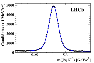
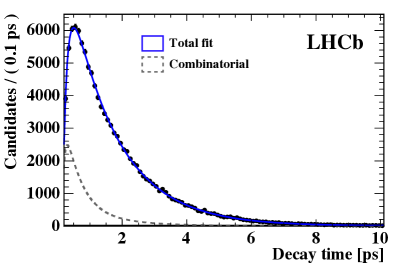
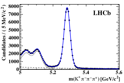
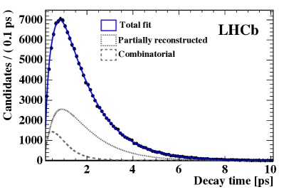
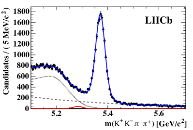
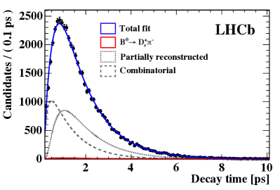
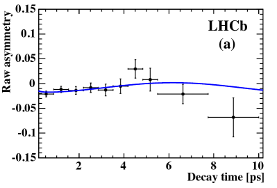
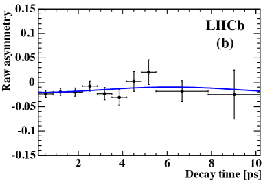
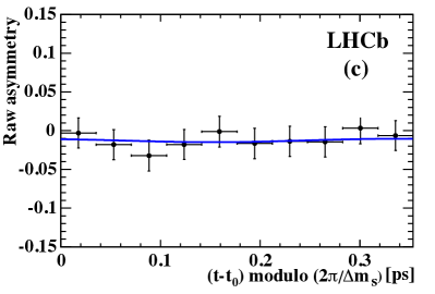
Figure 1 shows the , and invariant mass and decay time distributions, with the results of the global fits overlaid. Figure 2 shows the raw asymmetries, defined as the ratios between the difference and the sum of the overall decay time distributions, as a function of decay time for candidates in the signal mass region. The signal yields, values and detection asymmetries obtained from the global fits are reported in Table LABEL:tab:globalfit. The values obtained from the global fits are not well defined physical quantities, because efficiency corrections as a function of and need to be applied. They are reported here for illustrative purposes only.
| Parameter | |||
|---|---|---|---|
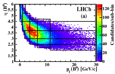
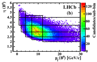
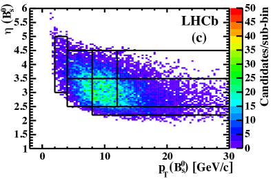
Figure 3 shows the two-dimensional distributions of (, ) for , and decays. The background components are subtracted using the sPlot technique [23] and the chosen definition of the various kinematic bins is overlaid. For the two decays we use a common set of bins, as reported in Table 3, in order to allow a simple combination of the two independent measurements. In the case of the , two additional bins at small and large are also defined. An accurate knowledge of the decay time resolution is important for decay, due to the fast oscillation of the meson. For this reason we determine the decay time resolution using the method previously described, applied to events belonging to each (, ) bin, where a double Gaussian function with zero mean and values of the widths depending on the given bin is used.
6 Systematic uncertainties
Several sources of systematic uncertainty that affect the determination of the production asymmetries are considered. For the invariant mass model, the effects of the uncertainty on the shapes of all components (signals, combinatorial and partially reconstructed backgrounds) are investigated. For the decay time model, systematic effects related to the decay time resolution and acceptance are studied. The effects of the uncertainties on the external inputs used in the fits, reported in Table 1, are evaluated by repeating the fits with each parameter varied by . Alternative parameterizations of the background components are also considered. To estimate the contribution of each single source, we repeat the fit for each (, ) bin after having modified the baseline fit model. The shifts from the relevant baseline values are taken as the systematic uncertainties. To estimate a systematic uncertainty related to the parameterization of final state radiation effects on the signal mass distributions, the parameter of Eq. 2 is varied by of the corresponding value obtained from fits to simulated events. A systematic uncertainty related to the invariant mass resolution model is estimated by repeating the fit using a single Gaussian function. The systematic uncertainty related to the parameterization of the mass shape for the combinatorial background is investigated by replacing the exponential function with a straight line. Concerning the partially reconstructed background, we assess a systematic uncertainty by repeating the fits while excluding the low mass sideband, i.e. applying the requirements for the decays and for decays. To estimate the uncertainty related to the parameterization of signal decay time acceptances, different acceptance functions are considered. Effects of inaccuracies in the knowledge of the decay time resolution are estimated by rescaling the widths of the baseline model to obtain an average resolution width differing by . Simulation studies also indicate that there is a small bias in the reconstructed decay time. The impact of such a bias is assessed by introducing a corresponding bias of in the decay time resolution model.
The determination of the systematic uncertainties related to the input value needs a special treatment, as is correlated with . For this reason, any variation of turns into the same shift of in each of the kinematic bins. Such a correlation is taken into account when averaging measurements from and decays, or when integrating over and . The values of the systematic uncertainties related to the knowledge of are 0.0013 in the case of and 0.0030 in the case of . The dominant systematic uncertainties for the decay are related to the signal mass shape and to . For the decay, the most relevant systematic uncertainties are related to the signal mass shape and to the partially reconstructed background. Systematic uncertainties associated with the decay time resolution and are the main sources for the decay.
7 Results
The values of are determined independently for and decays in each kinematic bin and then averaged. Table 3 reports the final results. The overall bin-by-bin agreement between the two sets of independent measurements is evaluated by means of a test, with a for degrees of freedom. The values of determined from the fits are reported in Table 4.
| () | ||||
|---|---|---|---|---|
| () | ||
|---|---|---|
The integration over and of the bin-by-bin values is performed within the ranges and . The integrated value of is given by
| (7) |
where the index runs over the bins, is the number of signal events and is the efficiency, defined as the number of selected events divided by the number of produced events in the i-th bin. The signal yield in each bin can be expressed as
| (8) |
where is the integrated luminosity, is the cross section, is the hadronization fraction, is the fraction of mesons produced in the i-th bin and is the branching fraction of the decay. By substituting from Eq. 8 into Eq. 7, the integrated value of becomes
| (9) |
where . The values of are determined using simulated events. The difference between the values of predicted by Pythia for and mesons is found to be negligible, if the same bins in and would be used.
| () | |||
|---|---|---|---|
These values are also extracted from data using decays. In this case is measured as
| (10) |
where is the yield in the i-th bin and is total reconstruction efficiency. The values of are determined using both simulated events and data control samples. The values of and , summarized in Table 5, exhibit systematic differences at the 10% level. The difference in the central value between calculated using either or is found to be 0.0024 using the binning scheme, and 0.0034 using the binning scheme. These values are assigned as systematic uncertainties for and . Table 6 summarizes the systematic uncertainties associated with the integrated measurements. In the first row, the combined systematic uncertainties estimated in each bin, as described in the previous section, are reported.
| Source | Uncertainty | |
|---|---|---|
| Combined systematic uncertainties from bin studies | 0.0004 | 0.0048 |
| Uncertainty on | 0.0013 | 0.0030 |
| Difference between and | 0.0024 | 0.0034 |
| Total | 0.0028 | 0.0066 |
Using Eq. 9, the integrated measurements of for and decays are found to be
which lead to the average
The integrated value of is
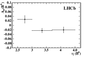
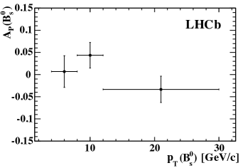
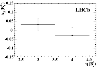
Finally, the dependencies of and on , obtained by integrating over , and on , obtained by integrating over , are shown in Fig. 4. The corresponding numerical values are reported in Tables 7 and 8.
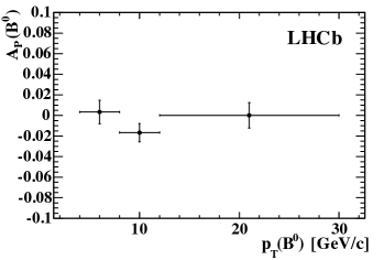
| Variable | Bin | |
|---|---|---|
| () | ||
| Variable | Bin | |
| () | ||
| (2.5, 3.5) | ||
| (3.5, 4.5) |
8 Conclusions
The production asymmetries of and mesons have been measured in collisions at within the acceptance of the LHCb detector, using a data sample corresponding to an integrated luminosity of 1.0. The measurements have been performed in bins of and , and provide constraints that can be used to test different models of -meson production. Furthermore, once integrated using appropriate weights for any reconstructed decay mode, they can be used to derive effective production asymmetries, as inputs for violation measurements with the LHCb detector.
The values of the production asymmetries integrated in the ranges and have been determined to be
where the first uncertainties are statistical and the second systematic. No clear evidence of dependences on the values of and has been observed.
9 Acknowledgments
We express our gratitude to our colleagues in the CERN accelerator departments for the excellent performance of the LHC. We thank the technical and administrative staff at the LHCb institutes. We acknowledge support from CERN and from the national agencies: CAPES, CNPq, FAPERJ and FINEP (Brazil); NSFC (China); CNRS/IN2P3 (France); BMBF, DFG, HGF and MPG (Germany); SFI (Ireland); INFN (Italy); FOM and NWO (The Netherlands); MNiSW and NCN (Poland); MEN/IFA (Romania); MinES and FANO (Russia); MinECo (Spain); SNSF and SER (Switzerland); NASU (Ukraine); STFC (United Kingdom); NSF (USA). The Tier1 computing centres are supported by IN2P3 (France), KIT and BMBF (Germany), INFN (Italy), NWO and SURF (The Netherlands), PIC (Spain), GridPP (United Kingdom). We are indebted to the communities behind the multiple open source software packages on which we depend. We are also thankful for the computing resources and the access to software R&D tools provided by Yandex LLC (Russia). Individual groups or members have received support from EPLANET, Marie Skłodowska-Curie Actions and ERC (European Union), Conseil général de Haute-Savoie, Labex ENIGMASS and OCEVU, Région Auvergne (France), RFBR (Russia), XuntaGal and GENCAT (Spain), Royal Society and Royal Commission for the Exhibition of 1851 (United Kingdom).
References
- [1] M. Chaichian and A. Fridman, On a possibility for measuring effects of CP violation at colliders, Phys. Lett. B298 (1993) 218
- [2] E. Norrbin and R. Vogt, Bottom production asymmetries at the LHC, arXiv:hep-ph/0003056
- [3] E. Norrbin and T. Sjöstrand, Production and hadronization of heavy quarks, Eur. Phys. J. C17 (2000) 137, arXiv:hep-ph/0005110
- [4] LHCb collaboration, R. Aaij et al., Measurement of the production asymmetry in 7 TeV collisions, Phys. Lett. B718 (2013) 902, arXiv:1210.4112
- [5] LHCb collaboration, R. Aaij et al., Measurement of the production asymmetry in 7 TeV pp collisions, Phys. Lett. B713 (2012) 186, arXiv:1205.0897
- [6] LHCb collaboration, A. A. Alves Jr. et al., The LHCb detector at the LHC, JINST 3 (2008) S08005
- [7] Particle Data Group, J. Beringer et al., Review of particle physics, Phys. Rev. D86 (2012) 010001, and 2013 partial update for the 2014 edition
- [8] V. V. Gligorov and M. Williams, Efficient, reliable and fast high-level triggering using a bonsai boosted decision tree, JINST 8 (2013) P02013, arXiv:1210.6861
- [9] T. Sjöstrand, S. Mrenna, and P. Skands, PYTHIA 6.4 physics and manual, JHEP 05 (2006) 026, arXiv:hep-ph/0603175
- [10] I. Belyaev et al., Handling of the generation of primary events in Gauss, the LHCb simulation framework, Nuclear Science Symposium Conference Record (NSS/MIC) IEEE (2010) 1155
- [11] GEANT4 collaboration, J. Allison et al., Geant4 developments and applications, IEEE Trans. Nucl. Sci. 53 (2006) 270
- [12] GEANT4 collaboration, S. Agostinelli et al., GEANT4: A simulation toolkit, Nucl. Instrum. Meth. A506 (2003) 250
- [13] M. Clemencic et al., The LHCb simulation application, Gauss: design, evolution and experience, J. Phys. Conf. Ser. 331 (2011) 032023
- [14] W. D. Hulsbergen, Decay chain fitting with a Kalman filter, Nucl. Instrum. Meth. A552 (2005) 566, arXiv:physics/0503191
- [15] L. Breiman, J. H. Friedman, R. A. Olshen, and C. J. Stone, Classification and regression trees, Wadsworth international group, Belmont, California, USA, 1984
- [16] R. E. Schapire and Y. Freund, A decision-theoretic generalization of on-line learning and an application to boosting, Jour. Comp. and Syst. Sc. 55 (1997) 119
- [17] K. S. Cranmer, Kernel estimation in high-energy physics, Comput. Phys. Commun. 136 (2001) 198, arXiv:hep-ex/0011057
- [18] LHCb collaboration, R. Aaij et al., Measurement of the fragmentation fraction ratio and its dependence on meson kinematics, JHEP 04 (2013) 001, arXiv:1301.5286
- [19] LHCb collaboration, R. Aaij et al., Measurement of hadron production fractions in 7 TeV collisions, Phys. Rev. D85 (2012) 032008, arXiv:1111.2357
- [20] LHCb collaboration, R. Aaij et al., Precision measurement of the - oscillation frequency with the decay , New J. Phys. 15 (2013) 053021, arXiv:1304.4741
- [21] Heavy Flavor Averaging Group, Y. Amhis et al., Averages of -hadron, -hadron, and -lepton properties as of early 2012, arXiv:1207.1158, update available online at http://www.slac.stanford.edu/xorg/hfag
- [22] LHCb collaboration, R. Aaij et al., Measurement of the flavour-specific -violating asymmetry in decays, Phys. Lett. B728 (2014) 607, arXiv:1308.1048
- [23] M. Pivk and F. R. Le Diberder, sPlot: a statistical tool to unfold data distributions, Nucl. Instrum. Meth. A555 (2005) 356, arXiv:physics/0402083
LHCb collaboration
R. Aaij41,
B. Adeva37,
M. Adinolfi46,
A. Affolder52,
Z. Ajaltouni5,
S. Akar6,
J. Albrecht9,
F. Alessio38,
M. Alexander51,
S. Ali41,
G. Alkhazov30,
P. Alvarez Cartelle37,
A.A. Alves Jr25,38,
S. Amato2,
S. Amerio22,
Y. Amhis7,
L. An3,
L. Anderlini17,g,
J. Anderson40,
R. Andreassen57,
M. Andreotti16,f,
J.E. Andrews58,
R.B. Appleby54,
O. Aquines Gutierrez10,
F. Archilli38,
A. Artamonov35,
M. Artuso59,
E. Aslanides6,
G. Auriemma25,n,
M. Baalouch5,
S. Bachmann11,
J.J. Back48,
A. Badalov36,
W. Baldini16,
R.J. Barlow54,
C. Barschel38,
S. Barsuk7,
W. Barter47,
V. Batozskaya28,
V. Battista39,
A. Bay39,
L. Beaucourt4,
J. Beddow51,
F. Bedeschi23,
I. Bediaga1,
S. Belogurov31,
K. Belous35,
I. Belyaev31,
E. Ben-Haim8,
G. Bencivenni18,
S. Benson38,
J. Benton46,
A. Berezhnoy32,
R. Bernet40,
M.-O. Bettler47,
M. van Beuzekom41,
A. Bien11,
S. Bifani45,
T. Bird54,
A. Bizzeti17,i,
P.M. Bjørnstad54,
T. Blake48,
F. Blanc39,
J. Blouw10,
S. Blusk59,
V. Bocci25,
A. Bondar34,
N. Bondar30,38,
W. Bonivento15,38,
S. Borghi54,
A. Borgia59,
M. Borsato7,
T.J.V. Bowcock52,
E. Bowen40,
C. Bozzi16,
T. Brambach9,
J. van den Brand42,
J. Bressieux39,
D. Brett54,
M. Britsch10,
T. Britton59,
J. Brodzicka54,
N.H. Brook46,
H. Brown52,
A. Bursche40,
G. Busetto22,r,
J. Buytaert38,
S. Cadeddu15,
R. Calabrese16,f,
M. Calvi20,k,
M. Calvo Gomez36,p,
P. Campana18,38,
D. Campora Perez38,
A. Carbone14,d,
G. Carboni24,l,
R. Cardinale19,38,j,
A. Cardini15,
L. Carson50,
K. Carvalho Akiba2,
G. Casse52,
L. Cassina20,
L. Castillo Garcia38,
M. Cattaneo38,
Ch. Cauet9,
R. Cenci58,
M. Charles8,
Ph. Charpentier38,
M. Chefdeville4,
S. Chen54,
S.-F. Cheung55,
N. Chiapolini40,
M. Chrzaszcz40,26,
K. Ciba38,
X. Cid Vidal38,
G. Ciezarek53,
P.E.L. Clarke50,
M. Clemencic38,
H.V. Cliff47,
J. Closier38,
V. Coco38,
J. Cogan6,
E. Cogneras5,
L. Cojocariu29,
P. Collins38,
A. Comerma-Montells11,
A. Contu15,
A. Cook46,
M. Coombes46,
S. Coquereau8,
G. Corti38,
M. Corvo16,f,
I. Counts56,
B. Couturier38,
G.A. Cowan50,
D.C. Craik48,
M. Cruz Torres60,
S. Cunliffe53,
R. Currie50,
C. D’Ambrosio38,
J. Dalseno46,
P. David8,
P.N.Y. David41,
A. Davis57,
K. De Bruyn41,
S. De Capua54,
M. De Cian11,
J.M. De Miranda1,
L. De Paula2,
W. De Silva57,
P. De Simone18,
D. Decamp4,
M. Deckenhoff9,
L. Del Buono8,
N. Déléage4,
D. Derkach55,
O. Deschamps5,
F. Dettori38,
A. Di Canto38,
H. Dijkstra38,
S. Donleavy52,
F. Dordei11,
M. Dorigo39,
A. Dosil Suárez37,
D. Dossett48,
A. Dovbnya43,
K. Dreimanis52,
G. Dujany54,
F. Dupertuis39,
P. Durante38,
R. Dzhelyadin35,
A. Dziurda26,
A. Dzyuba30,
S. Easo49,38,
U. Egede53,
V. Egorychev31,
S. Eidelman34,
S. Eisenhardt50,
U. Eitschberger9,
R. Ekelhof9,
L. Eklund51,
I. El Rifai5,
Ch. Elsasser40,
S. Ely59,
S. Esen11,
H.-M. Evans47,
T. Evans55,
A. Falabella14,
C. Färber11,
C. Farinelli41,
N. Farley45,
S. Farry52,
RF Fay52,
D. Ferguson50,
V. Fernandez Albor37,
F. Ferreira Rodrigues1,
M. Ferro-Luzzi38,
S. Filippov33,
M. Fiore16,f,
M. Fiorini16,f,
M. Firlej27,
C. Fitzpatrick39,
T. Fiutowski27,
M. Fontana10,
F. Fontanelli19,j,
R. Forty38,
O. Francisco2,
M. Frank38,
C. Frei38,
M. Frosini17,38,g,
J. Fu21,38,
E. Furfaro24,l,
A. Gallas Torreira37,
D. Galli14,d,
S. Gallorini22,
S. Gambetta19,j,
M. Gandelman2,
P. Gandini59,
Y. Gao3,
J. García Pardiñas37,
J. Garofoli59,
J. Garra Tico47,
L. Garrido36,
C. Gaspar38,
R. Gauld55,
L. Gavardi9,
G. Gavrilov30,
A. Geraci21,v,
E. Gersabeck11,
M. Gersabeck54,
T. Gershon48,
Ph. Ghez4,
A. Gianelle22,
S. Giani’39,
V. Gibson47,
L. Giubega29,
V.V. Gligorov38,
C. Göbel60,
D. Golubkov31,
A. Golutvin53,31,38,
A. Gomes1,a,
C. Gotti20,
M. Grabalosa Gándara5,
R. Graciani Diaz36,
L.A. Granado Cardoso38,
E. Graugés36,
G. Graziani17,
A. Grecu29,
E. Greening55,
S. Gregson47,
P. Griffith45,
L. Grillo11,
O. Grünberg62,
B. Gui59,
E. Gushchin33,
Yu. Guz35,38,
T. Gys38,
C. Hadjivasiliou59,
G. Haefeli39,
C. Haen38,
S.C. Haines47,
S. Hall53,
B. Hamilton58,
T. Hampson46,
X. Han11,
S. Hansmann-Menzemer11,
N. Harnew55,
S.T. Harnew46,
J. Harrison54,
J. He38,
T. Head38,
V. Heijne41,
K. Hennessy52,
P. Henrard5,
L. Henry8,
J.A. Hernando Morata37,
E. van Herwijnen38,
M. Heß62,
A. Hicheur1,
D. Hill55,
M. Hoballah5,
C. Hombach54,
W. Hulsbergen41,
P. Hunt55,
N. Hussain55,
D. Hutchcroft52,
D. Hynds51,
M. Idzik27,
P. Ilten56,
R. Jacobsson38,
A. Jaeger11,
J. Jalocha55,
E. Jans41,
P. Jaton39,
A. Jawahery58,
F. Jing3,
M. John55,
D. Johnson55,
C.R. Jones47,
C. Joram38,
B. Jost38,
N. Jurik59,
M. Kaballo9,
S. Kandybei43,
W. Kanso6,
M. Karacson38,
T.M. Karbach38,
S. Karodia51,
M. Kelsey59,
I.R. Kenyon45,
T. Ketel42,
B. Khanji20,
C. Khurewathanakul39,
S. Klaver54,
K. Klimaszewski28,
O. Kochebina7,
M. Kolpin11,
I. Komarov39,
R.F. Koopman42,
P. Koppenburg41,38,
M. Korolev32,
A. Kozlinskiy41,
L. Kravchuk33,
K. Kreplin11,
M. Kreps48,
G. Krocker11,
P. Krokovny34,
F. Kruse9,
W. Kucewicz26,o,
M. Kucharczyk20,26,38,k,
V. Kudryavtsev34,
K. Kurek28,
T. Kvaratskheliya31,
V.N. La Thi39,
D. Lacarrere38,
G. Lafferty54,
A. Lai15,
D. Lambert50,
R.W. Lambert42,
G. Lanfranchi18,
C. Langenbruch48,
B. Langhans38,
T. Latham48,
C. Lazzeroni45,
R. Le Gac6,
J. van Leerdam41,
J.-P. Lees4,
R. Lefèvre5,
A. Leflat32,
J. Lefrançois7,
S. Leo23,
O. Leroy6,
T. Lesiak26,
B. Leverington11,
Y. Li3,
T. Likhomanenko63,
M. Liles52,
R. Lindner38,
C. Linn38,
F. Lionetto40,
B. Liu15,
S. Lohn38,
I. Longstaff51,
J.H. Lopes2,
N. Lopez-March39,
P. Lowdon40,
H. Lu3,
D. Lucchesi22,r,
H. Luo50,
A. Lupato22,
E. Luppi16,f,
O. Lupton55,
F. Machefert7,
I.V. Machikhiliyan31,
F. Maciuc29,
O. Maev30,
S. Malde55,
A. Malinin63,
G. Manca15,e,
G. Mancinelli6,
A. Mapelli38,
J. Maratas5,
J.F. Marchand4,
U. Marconi14,
C. Marin Benito36,
P. Marino23,t,
R. Märki39,
J. Marks11,
G. Martellotti25,
A. Martens8,
A. Martín Sánchez7,
M. Martinelli39,
D. Martinez Santos42,
F. Martinez Vidal64,
D. Martins Tostes2,
A. Massafferri1,
R. Matev38,
Z. Mathe38,
C. Matteuzzi20,
A. Mazurov16,f,
M. McCann53,
J. McCarthy45,
A. McNab54,
R. McNulty12,
B. McSkelly52,
B. Meadows57,
F. Meier9,
M. Meissner11,
M. Merk41,
D.A. Milanes8,
M.-N. Minard4,
N. Moggi14,
J. Molina Rodriguez60,
S. Monteil5,
M. Morandin22,
P. Morawski27,
A. Mordà6,
M.J. Morello23,t,
J. Moron27,
A.-B. Morris50,
R. Mountain59,
F. Muheim50,
K. Müller40,
M. Mussini14,
B. Muster39,
P. Naik46,
T. Nakada39,
R. Nandakumar49,
I. Nasteva2,
M. Needham50,
N. Neri21,
S. Neubert38,
N. Neufeld38,
M. Neuner11,
A.D. Nguyen39,
T.D. Nguyen39,
C. Nguyen-Mau39,q,
M. Nicol7,
V. Niess5,
R. Niet9,
N. Nikitin32,
T. Nikodem11,
A. Novoselov35,
D.P. O’Hanlon48,
A. Oblakowska-Mucha27,
V. Obraztsov35,
S. Oggero41,
S. Ogilvy51,
O. Okhrimenko44,
R. Oldeman15,e,
G. Onderwater65,
M. Orlandea29,
J.M. Otalora Goicochea2,
P. Owen53,
A. Oyanguren64,
B.K. Pal59,
A. Palano13,c,
F. Palombo21,u,
M. Palutan18,
J. Panman38,
A. Papanestis49,38,
M. Pappagallo51,
L.L. Pappalardo16,f,
C. Parkes54,
C.J. Parkinson9,45,
G. Passaleva17,
G.D. Patel52,
M. Patel53,
C. Patrignani19,j,
A. Pazos Alvarez37,
A. Pearce54,
A. Pellegrino41,
M. Pepe Altarelli38,
S. Perazzini14,d,
E. Perez Trigo37,
P. Perret5,
M. Perrin-Terrin6,
L. Pescatore45,
E. Pesen66,
K. Petridis53,
A. Petrolini19,j,
E. Picatoste Olloqui36,
B. Pietrzyk4,
T. Pilař48,
D. Pinci25,
A. Pistone19,
S. Playfer50,
M. Plo Casasus37,
F. Polci8,
A. Poluektov48,34,
E. Polycarpo2,
A. Popov35,
D. Popov10,
B. Popovici29,
C. Potterat2,
E. Price46,
J. Prisciandaro39,
A. Pritchard52,
C. Prouve46,
V. Pugatch44,
A. Puig Navarro39,
G. Punzi23,s,
W. Qian4,
B. Rachwal26,
J.H. Rademacker46,
B. Rakotomiaramanana39,
M. Rama18,
M.S. Rangel2,
I. Raniuk43,
N. Rauschmayr38,
G. Raven42,
S. Reichert54,
M.M. Reid48,
A.C. dos Reis1,
S. Ricciardi49,
S. Richards46,
M. Rihl38,
K. Rinnert52,
V. Rives Molina36,
D.A. Roa Romero5,
P. Robbe7,
A.B. Rodrigues1,
E. Rodrigues54,
P. Rodriguez Perez54,
S. Roiser38,
V. Romanovsky35,
A. Romero Vidal37,
M. Rotondo22,
J. Rouvinet39,
T. Ruf38,
H. Ruiz36,
P. Ruiz Valls64,
J.J. Saborido Silva37,
N. Sagidova30,
P. Sail51,
B. Saitta15,e,
V. Salustino Guimaraes2,
C. Sanchez Mayordomo64,
B. Sanmartin Sedes37,
R. Santacesaria25,
C. Santamarina Rios37,
E. Santovetti24,l,
A. Sarti18,m,
C. Satriano25,n,
A. Satta24,
D.M. Saunders46,
M. Savrie16,f,
D. Savrina31,32,
M. Schiller42,
H. Schindler38,
M. Schlupp9,
M. Schmelling10,
B. Schmidt38,
O. Schneider39,
A. Schopper38,
M.-H. Schune7,
R. Schwemmer38,
B. Sciascia18,
A. Sciubba25,
M. Seco37,
A. Semennikov31,
I. Sepp53,
N. Serra40,
J. Serrano6,
L. Sestini22,
P. Seyfert11,
M. Shapkin35,
I. Shapoval16,43,f,
Y. Shcheglov30,
T. Shears52,
L. Shekhtman34,
V. Shevchenko63,
A. Shires9,
R. Silva Coutinho48,
G. Simi22,
M. Sirendi47,
N. Skidmore46,
T. Skwarnicki59,
N.A. Smith52,
E. Smith55,49,
E. Smith53,
J. Smith47,
M. Smith54,
H. Snoek41,
M.D. Sokoloff57,
F.J.P. Soler51,
F. Soomro39,
D. Souza46,
B. Souza De Paula2,
B. Spaan9,
A. Sparkes50,
P. Spradlin51,
S. Sridharan38,
F. Stagni38,
M. Stahl11,
S. Stahl11,
O. Steinkamp40,
O. Stenyakin35,
S. Stevenson55,
S. Stoica29,
S. Stone59,
B. Storaci40,
S. Stracka23,38,
M. Straticiuc29,
U. Straumann40,
R. Stroili22,
V.K. Subbiah38,
L. Sun57,
W. Sutcliffe53,
K. Swientek27,
S. Swientek9,
V. Syropoulos42,
M. Szczekowski28,
P. Szczypka39,38,
D. Szilard2,
T. Szumlak27,
S. T’Jampens4,
M. Teklishyn7,
G. Tellarini16,f,
F. Teubert38,
C. Thomas55,
E. Thomas38,
J. van Tilburg41,
V. Tisserand4,
M. Tobin39,
S. Tolk42,
L. Tomassetti16,f,
D. Tonelli38,
S. Topp-Joergensen55,
N. Torr55,
E. Tournefier4,
S. Tourneur39,
M.T. Tran39,
M. Tresch40,
A. Tsaregorodtsev6,
P. Tsopelas41,
N. Tuning41,
M. Ubeda Garcia38,
A. Ukleja28,
A. Ustyuzhanin63,
U. Uwer11,
V. Vagnoni14,
G. Valenti14,
A. Vallier7,
R. Vazquez Gomez18,
P. Vazquez Regueiro37,
C. Vázquez Sierra37,
S. Vecchi16,
J.J. Velthuis46,
M. Veltri17,h,
G. Veneziano39,
M. Vesterinen11,
B. Viaud7,
D. Vieira2,
M. Vieites Diaz37,
X. Vilasis-Cardona36,p,
A. Vollhardt40,
D. Volyanskyy10,
D. Voong46,
A. Vorobyev30,
V. Vorobyev34,
C. Voß62,
H. Voss10,
J.A. de Vries41,
R. Waldi62,
C. Wallace48,
R. Wallace12,
J. Walsh23,
S. Wandernoth11,
J. Wang59,
D.R. Ward47,
N.K. Watson45,
D. Websdale53,
M. Whitehead48,
J. Wicht38,
D. Wiedner11,
G. Wilkinson55,
M.P. Williams45,
M. Williams56,
F.F. Wilson49,
J. Wimberley58,
J. Wishahi9,
W. Wislicki28,
M. Witek26,
G. Wormser7,
S.A. Wotton47,
S. Wright47,
S. Wu3,
K. Wyllie38,
Y. Xie61,
Z. Xing59,
Z. Xu39,
Z. Yang3,
X. Yuan3,
O. Yushchenko35,
M. Zangoli14,
M. Zavertyaev10,b,
L. Zhang59,
W.C. Zhang12,
Y. Zhang3,
A. Zhelezov11,
A. Zhokhov31,
L. Zhong3,
A. Zvyagin38.
1Centro Brasileiro de Pesquisas Físicas (CBPF), Rio de Janeiro, Brazil
2Universidade Federal do Rio de Janeiro (UFRJ), Rio de Janeiro, Brazil
3Center for High Energy Physics, Tsinghua University, Beijing, China
4LAPP, Université de Savoie, CNRS/IN2P3, Annecy-Le-Vieux, France
5Clermont Université, Université Blaise Pascal, CNRS/IN2P3, LPC, Clermont-Ferrand, France
6CPPM, Aix-Marseille Université, CNRS/IN2P3, Marseille, France
7LAL, Université Paris-Sud, CNRS/IN2P3, Orsay, France
8LPNHE, Université Pierre et Marie Curie, Université Paris Diderot, CNRS/IN2P3, Paris, France
9Fakultät Physik, Technische Universität Dortmund, Dortmund, Germany
10Max-Planck-Institut für Kernphysik (MPIK), Heidelberg, Germany
11Physikalisches Institut, Ruprecht-Karls-Universität Heidelberg, Heidelberg, Germany
12School of Physics, University College Dublin, Dublin, Ireland
13Sezione INFN di Bari, Bari, Italy
14Sezione INFN di Bologna, Bologna, Italy
15Sezione INFN di Cagliari, Cagliari, Italy
16Sezione INFN di Ferrara, Ferrara, Italy
17Sezione INFN di Firenze, Firenze, Italy
18Laboratori Nazionali dell’INFN di Frascati, Frascati, Italy
19Sezione INFN di Genova, Genova, Italy
20Sezione INFN di Milano Bicocca, Milano, Italy
21Sezione INFN di Milano, Milano, Italy
22Sezione INFN di Padova, Padova, Italy
23Sezione INFN di Pisa, Pisa, Italy
24Sezione INFN di Roma Tor Vergata, Roma, Italy
25Sezione INFN di Roma La Sapienza, Roma, Italy
26Henryk Niewodniczanski Institute of Nuclear Physics Polish Academy of Sciences, Kraków, Poland
27AGH - University of Science and Technology, Faculty of Physics and Applied Computer Science, Kraków, Poland
28National Center for Nuclear Research (NCBJ), Warsaw, Poland
29Horia Hulubei National Institute of Physics and Nuclear Engineering, Bucharest-Magurele, Romania
30Petersburg Nuclear Physics Institute (PNPI), Gatchina, Russia
31Institute of Theoretical and Experimental Physics (ITEP), Moscow, Russia
32Institute of Nuclear Physics, Moscow State University (SINP MSU), Moscow, Russia
33Institute for Nuclear Research of the Russian Academy of Sciences (INR RAN), Moscow, Russia
34Budker Institute of Nuclear Physics (SB RAS) and Novosibirsk State University, Novosibirsk, Russia
35Institute for High Energy Physics (IHEP), Protvino, Russia
36Universitat de Barcelona, Barcelona, Spain
37Universidad de Santiago de Compostela, Santiago de Compostela, Spain
38European Organization for Nuclear Research (CERN), Geneva, Switzerland
39Ecole Polytechnique Fédérale de Lausanne (EPFL), Lausanne, Switzerland
40Physik-Institut, Universität Zürich, Zürich, Switzerland
41Nikhef National Institute for Subatomic Physics, Amsterdam, The Netherlands
42Nikhef National Institute for Subatomic Physics and VU University Amsterdam, Amsterdam, The Netherlands
43NSC Kharkiv Institute of Physics and Technology (NSC KIPT), Kharkiv, Ukraine
44Institute for Nuclear Research of the National Academy of Sciences (KINR), Kyiv, Ukraine
45University of Birmingham, Birmingham, United Kingdom
46H.H. Wills Physics Laboratory, University of Bristol, Bristol, United Kingdom
47Cavendish Laboratory, University of Cambridge, Cambridge, United Kingdom
48Department of Physics, University of Warwick, Coventry, United Kingdom
49STFC Rutherford Appleton Laboratory, Didcot, United Kingdom
50School of Physics and Astronomy, University of Edinburgh, Edinburgh, United Kingdom
51School of Physics and Astronomy, University of Glasgow, Glasgow, United Kingdom
52Oliver Lodge Laboratory, University of Liverpool, Liverpool, United Kingdom
53Imperial College London, London, United Kingdom
54School of Physics and Astronomy, University of Manchester, Manchester, United Kingdom
55Department of Physics, University of Oxford, Oxford, United Kingdom
56Massachusetts Institute of Technology, Cambridge, MA, United States
57University of Cincinnati, Cincinnati, OH, United States
58University of Maryland, College Park, MD, United States
59Syracuse University, Syracuse, NY, United States
60Pontifícia Universidade Católica do Rio de Janeiro (PUC-Rio), Rio de Janeiro, Brazil, associated to 2
61Institute of Particle Physics, Central China Normal University, Wuhan, Hubei, China, associated to 3
62Institut für Physik, Universität Rostock, Rostock, Germany, associated to 11
63National Research Centre Kurchatov Institute, Moscow, Russia, associated to 31
64Instituto de Fisica Corpuscular (IFIC), Universitat de Valencia-CSIC, Valencia, Spain, associated to 36
65KVI - University of Groningen, Groningen, The Netherlands, associated to 41
66Celal Bayar University, Manisa, Turkey, associated to 38
aUniversidade Federal do Triângulo Mineiro (UFTM), Uberaba-MG, Brazil
bP.N. Lebedev Physical Institute, Russian Academy of Science (LPI RAS), Moscow, Russia
cUniversità di Bari, Bari, Italy
dUniversità di Bologna, Bologna, Italy
eUniversità di Cagliari, Cagliari, Italy
fUniversità di Ferrara, Ferrara, Italy
gUniversità di Firenze, Firenze, Italy
hUniversità di Urbino, Urbino, Italy
iUniversità di Modena e Reggio Emilia, Modena, Italy
jUniversità di Genova, Genova, Italy
kUniversità di Milano Bicocca, Milano, Italy
lUniversità di Roma Tor Vergata, Roma, Italy
mUniversità di Roma La Sapienza, Roma, Italy
nUniversità della Basilicata, Potenza, Italy
oAGH - University of Science and Technology, Faculty of Computer Science, Electronics and Telecommunications, Kraków, Poland
pLIFAELS, La Salle, Universitat Ramon Llull, Barcelona, Spain
qHanoi University of Science, Hanoi, Viet Nam
rUniversità di Padova, Padova, Italy
sUniversità di Pisa, Pisa, Italy
tScuola Normale Superiore, Pisa, Italy
uUniversità degli Studi di Milano, Milano, Italy
vPolitecnico di Milano, Milano, Italy