The Proton Radius from Bayesian Inference
Abstract
The methods of Bayesian statistics are used to extract the value of the proton radius from the elastic scattering data in a model independent way. To achieve that goal a large number of parametrizations (equivalent to neural network schemes) are considered and ranked by their conditional probability instead of using the minimal error criterion. As a result the most probable proton radii values ( fm, fm) are obtained and systematic error due to freedom in the choice of parametrization is estimated. Correcting the data for the two photon exchange effect leads to smaller difference between the extracted values of and . The results disagree with recent muonic atom measurements.
pacs:
13.40.Gp, 25.30.Bf, 14.20.Dh, 84.35.+iThe problem of the proton radius is being discussed in the particle and atomic physics for many years but recently it has received even more attention due to the new results coming form the Lamb shift measurements of the muonic hydrogen atom () Pohl et al. (2010). It is a very accurate estimate of the proton radius but it is inconsistent with the CODATA value (compilation of the measurements in hydrogen atom and analysis of the electron-proton scattering data) Mohr et al. (2012). This disagreement, called “the proton radius puzzle”, has not been explained yet. There are many proposals to resolve the problem including considering different types of interaction for and Kraus et al. (2014) or “weakening the assumptions of perturbative formulation of quantum electrodynamics within the proton” Pachucki and Meissner (2014). In this paper we introduce a novel approach to the extraction of the proton radius from the scattering data, which allows one to control the model dependence of the result within a Bayesian objective algorithm.
The electromagnetic (E-M) structure of the proton is encoded in the electric and magnetic form factors, which are also the crucial input for the atomic (hydrogen-like) calculations Pachucki (1996). In the low limit in the Breit frame they are related with the distributions of the electric charge and magnetic momentum inside the nucleon Ernst et al. (1960). In particular the nucleon radius is expressed by the slope of the form factors at vanishing :
| (1) |
The value of can be obtained from the scattering data (mainly elastic ). Recent results include Bernauer et al. (2010, 2013); Hill and Paz (2010); Lorenz et al. (2012); Lorenz and Meissner (2014) and a more complete list can be found in Refs. Epstein et al. (2014); Karshenboim (2014); Kraus et al. (2014). These analyses have been performed in the spirit of the frequentistic statistics.
The values of the proton radius (related to the electric charge distribution) obtained by different authors during the last fifty years, range from about 0.8 fm to about 0.9 fm Sick (2003). Indeed, as it was demonstrated in Hill and Paz (2010); Bernauer et al. (2013) the results depend the choice of the form factor parametrization but it is obvious that the collection of datasets used in the analysis also matters. Even the right choice of the number of parameters in a given class of parametrizations can be a challenge. More parameters in the fit can always reduce the error but at some point the fit tends to reproduce statical fluctuations of the experimental measurements. Such a model overfits the data i.e. describes existing points with unrealistic precision but has no predictive power – introducing new data points drastically increases the error and spoils the quality of the fit. This is connected with the so called bias variance trade-off. Some attempt to resolve this problem has been made in Ref. Hill and Paz (2010) where conformal mapping was used in order to exploit the analytic properties of the form factors.

Our philosophy is different. In contrast to the frequentistic statistics methods used in the above papers, we use the Bayesian statistics which is well suited to model comparison. Within this framework, adapted for neural networks, we select the most optimal model (according to the data) and extract the value of the proton radius.
The extraction of the nucleon form factors in Graczyk et al. (2010) was our first use of the Bayesian neural network framework. In the next paper Graczyk (2011) the approach was significantly improved to obtain the two-photon exchange (TPE) correction to unpolarized elastic cross section. However, because of some physical assumptions these analyses were not dedicated to the low- region. In the present paper we overcome this difficulty because: (i) the TPE contribution (elastic and inelastic described by box diagrams with nucleon and resonance as intermediate hadronic states) calculated in Graczyk (2013) is subtracted from the data and only E-M form factors are extracted from the cross section and polarization transfer data; (ii) the form factors are re-parameterized in order to automatically fulfil ( is the proton magnetic moment); (iii) our software has been significantly improved in terms of accuracy and efficiency.
Here we briefly outline the Bayesian framework, for more details see Graczyk et al. (2010); Graczyk (2011, 2013). The main idea is to consider a large class of models. By a model we mean the function used to fit the data and two conditional probabilities: – prior which accommodates the initial assumption about the , and the likelihood ; is the set of parameters of the function . Then the models are ranked by the conditional probability , which can be replaced by the evidence if the data is the same and no model is preferred at the beginning of the analysis.

For any given model we denote with the configuration of the parameters which maximizes the posterior
| (2) |
Finding in one of the steps of the analysis.
Usually the evidence is peaked at and it simplifies to the likelihood at the maximum multiplied by the Occam factor which makes too complex models less likely MacKay (1991)
| (3) |
where is the number of parameters and .
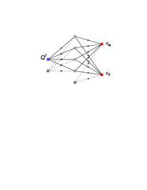
For the function we take the feed-forward neural networks with one hidden layer of units (Fig. 1), which correspond to linear combinations of sigmoid functions. This class of functions can be used to approximate any continuous function with arbitrary precision Cybenko (1989).
The prior function for the neural network parameters has the standard form . The parameter is the regularizer which determines the width of the initial Gaussian distribution for the parameters. In principle it should be treated as another parameter of the model and its optimal value is also obtained during the analysis.

The likelihood is defined by the distribution
| (4) |
The includes the unpolarized elastic scattering cross section data, which are assumed to be parametrized by one-photon exchange formula ( is the proton mass, denotes photon polarizability). Each independent set of cross section measurements is characterized by its systematic normalization uncertainty so we introduce a separate normalization parameter for every data set. Values of these parameters are obtained by an iterative algorithm described in Graczyk (2011). The includes the form factor ratio data from the polarization transfer measurements. We consider the same selection of data as in Graczyk (2011) with one additional data set from Zhan et al. (2011) and make the prior assumption that all data sets are equally relevant. The MAMI data Bernauer et al. (2010) are not included in the analysis because of the difficulties described in Arrington (2011).
The optimal configuration is found by an iterative procedure based on the fact that the maximum of the posterior corresponds to the minimum over of the error function and also , where
Eventually the logarithm of evidence for the model (in the Hessian approximation) reads:
| (5) | |||||
where and -s are the eigenvalues of the matrix .
As the form factors , describe the properties of the same object, they must be related, so we parametrize them with a single feed forward neural network with one input () and two outputs, and (see Fig. 1),
| (6) |
where and GeV2. Then the value of the proton radius is given by
| (7) |
where . We see that the network outputs at directly contribute to the deviation of the proton radius from the dipole form factor value.
In Refs. Rosenfelder (2000); Sick (2003) it was shown that modifying the cross section data by the Coulomb distortion (CD) is important in the extraction of the proton radius. On the other hand, the CD is a part of the TPE effect111The relevance of the TPE effect and higher order Born corrections in the proton radius extraction is also discussed in Refs. Gorchtein (2014) and Arrington (2013); Arrington and Sick (2004) respectively., which has to be subtracted from the data to obtain the form factors which agree with the polarization transfer measurements Arrington et al. (2007). Similarly as in Blunden and Sick (2005) we correct the cross section data by the TPE contribution (calculated in Graczyk (2013) in similar way as in Blunden et al. (2005); Kondratyuk et al. (2005)).
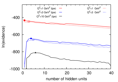
The set of all possible parametrizations is infinite. In our approach the models are grouped according to the number of units in the hidden layer. For each group we found the which maximize the evidence. The dependence of the maximal evidence on the number of hidden units is plotted in Fig. 2. For every analysis the evidence reaches a peak (which defines the best model) and then starts to fall. Because of this fact we do not consider the networks with more then 40 hidden units. The total number of obtained neural network parameterizations exceeded half million.
It needs to be underlined that the models which maximize the evidence are not those which minimize the . This is true in each class of models and also globally. The decreases with the number of parameters possibly saturating at some point. But the models with the lowest tend to overfit the data, which is one of the reasons why the is not a suitable criterion for ranking the models. The other problems of -based criteria are discussed in Kraus et al. (2014). Objective mathematical methods for model comparison are provided by the Bayesian statistics.
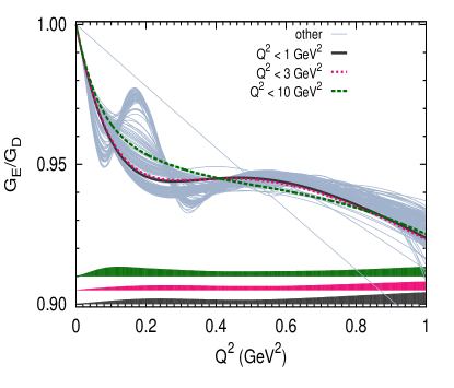
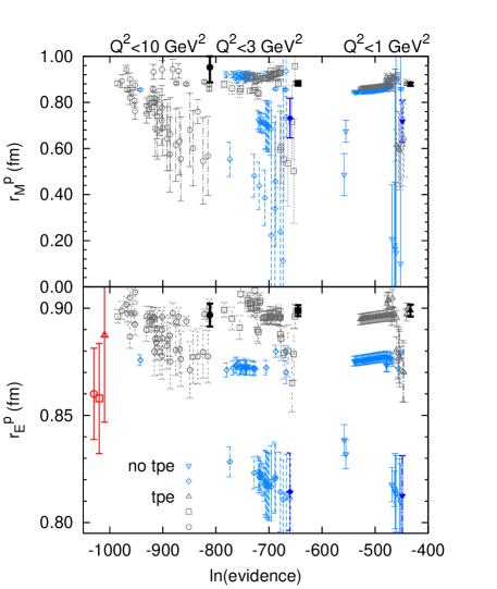
In Fig. 3 it is shown how the form factor plots depend on the choice of the parametrization. The gray lines correspond to the best models in each group, while the globally best for each analysis are shown with color. Certainly the choice of the form factor parametrization has also strong impact on the obtained proton radius value (Fig. 4). Hence it is crucial to have criterion for finding the model which is the most favorable by the measurements. On the other hand each model can be true with the probability (proportional to the evidence) so it is possible to calculate the expected value of the proton radius and the systematic uncertainty due to the choice of the model. In practice the expected value is very close to the most probable value (see Tables 1 and 2).
| (GeV2) | (fm) | (fm) | |
|---|---|---|---|
| 1 | |||
| 4 | |||
| 6 |
| (GeV2) | (fm) | (fm) |
|---|---|---|
In Fig. 4 we show the proton radii values obtained from the analyses where data points with above , and GeV2 are rejected (for the data uncorrected by the TPE we considered only GeV2). The choice of the value for the cutoff has small impact on the extraction of the proton radii. For the result of our analysis we take those from the lowest cut, namely fm and fm. On the other hand the ’s obtained based on the minimal error criterion depend on the cutoff choice. These results are smaller than those indicated by the evidence and have larger uncertainties, see Fig. 4. We leave for future studies within the Bayesian framework the quantitative investigation of the dependence of the results on the data set selection and value. Eventually it can be seen in Fig. 4 that using the data uncorrected by TPE effect leads to larger uncertainties of and and larger difference ( fm with TPE and fm without).

We would like to emphasize that according to our knowledge the present work is the first extraction of the proton radius based on the Bayesian methods. The extracted value of the proton radius agrees with previous results Sick (2003); Blunden and Sick (2005); Hill and Paz (2010) but disagrees with the muonic atom measurements Pohl et al. (2010). The subtracting of the TPE correction from the cross section data plays an important role in the analysis.
The calculations have been carried out in Wroclaw Centre for Networking and Supercomputing (http://www.wcss.wroc.pl), grant No. 268.
References
- Pohl et al. (2010) R. Pohl, A. Antognini, F. Nez, F. D. Amaro, F. Biraben, et al., Nature 466, 213 (2010).
- Mohr et al. (2012) P. J. Mohr, B. N. Taylor, and D. B. Newell, Rev.Mod.Phys. 84, 1527 (2012), arXiv:1203.5425 [physics.atom-ph] .
- Kraus et al. (2014) E. Kraus, K. Mesick, A. White, R. Gilman, and S. Strauch, (2014), arXiv:1405.4735 [nucl-ex] .
- Pachucki and Meissner (2014) K. Pachucki and K. A. Meissner, (2014), arXiv:1405.6582 [hep-ph] .
- Pachucki (1996) K. Pachucki, Phys.Rev. A53, 2092 (1996).
- Ernst et al. (1960) F. Ernst, R. Sachs, and K. Wali, Phys.Rev. 119, 1105 (1960).
- Bernauer et al. (2010) J. Bernauer et al. (A1 Collaboration), Phys.Rev.Lett. 105, 242001 (2010), arXiv:1007.5076 [nucl-ex] .
- Bernauer et al. (2013) J. Bernauer et al. (A1 Collaboration), (2013), 10.1103/PhysRevC.90.015206, arXiv:1307.6227 [nucl-ex] .
- Hill and Paz (2010) R. J. Hill and G. Paz, Phys.Rev. D82, 113005 (2010), arXiv:1008.4619 [hep-ph] .
- Lorenz et al. (2012) I. Lorenz, H.-W. Hammer, and U.-G. Meissner, Eur.Phys.J. A48, 151 (2012), arXiv:1205.6628 [hep-ph] .
- Lorenz and Meissner (2014) I. Lorenz and U. G. Meissner, (2014), arXiv:1406.2962 [hep-ph] .
- Epstein et al. (2014) Z. Epstein, G. Paz, and J. Roy, (2014), arXiv:1407.5683 [hep-ph] .
- Karshenboim (2014) S. G. Karshenboim, (2014), arXiv:1405.6515 [hep-ph] .
- Sick (2003) I. Sick, Phys.Lett. B576, 62 (2003), arXiv:nucl-ex/0310008 [nucl-ex] .
- Graczyk et al. (2010) K. M. Graczyk, P. Plonski, and R. Sulej, JHEP 1009, 053 (2010), arXiv:1006.0342 [hep-ph] .
- Graczyk (2011) K. M. Graczyk, Phys.Rev. C84, 034314 (2011), arXiv:1106.1204 [hep-ph] .
- Graczyk (2013) K. M. Graczyk, Phys.Rev. C88, 065205 (2013), arXiv:1306.5991 [hep-ph] .
- MacKay (1991) D. MacKay, Bayesian Methods for Adaptive Models, Ph.D. thesis, California Institute of Technology (1991).
- Cybenko (1989) G. Cybenko, Math Control, Signal 2, 303 (1989).
- Zhan et al. (2011) X. Zhan, K. Allada, D. Armstrong, J. Arrington, W. Bertozzi, et al., Phys.Lett. B705, 59 (2011), arXiv:1102.0318 [nucl-ex] .
- Arrington (2011) J. Arrington, Phys.Rev.Lett. 107, 119101 (2011), arXiv:1108.3058 [nucl-ex] .
- Rosenfelder (2000) R. Rosenfelder, Phys.Lett. B479, 381 (2000), arXiv:nucl-th/9912031 [nucl-th] .
- Gorchtein (2014) M. Gorchtein, (2014), arXiv:1406.1612 [nucl-th] .
- Arrington (2013) J. Arrington, J.Phys. G40, 115003 (2013), arXiv:1210.2677 [nucl-ex] .
- Arrington and Sick (2004) J. Arrington and I. Sick, Phys.Rev. C70, 028203 (2004), arXiv:nucl-ex/0406014 [nucl-ex] .
- Arrington et al. (2007) J. Arrington, W. Melnitchouk, and J. Tjon, Phys.Rev. C76, 035205 (2007), arXiv:0707.1861 [nucl-ex] .
- Blunden and Sick (2005) P. G. Blunden and I. Sick, Phys.Rev. C72, 057601 (2005), arXiv:nucl-th/0508037 [nucl-th] .
- Blunden et al. (2005) P. Blunden, W. Melnitchouk, and J. Tjon, Phys.Rev. C72, 034612 (2005), arXiv:nucl-th/0506039 [nucl-th] .
- Kondratyuk et al. (2005) S. Kondratyuk, P. Blunden, W. Melnitchouk, and J. Tjon, Phys.Rev.Lett. 95, 172503 (2005), arXiv:nucl-th/0506026 [nucl-th] .