Conditional Restricted Boltzmann Machines for Cold Start Recommendations
Abstract
Restricted Boltzman Machines (RBMs) have been successfully used in recommender systems. However, as with most of other collaborative filtering techniques, it cannot solve cold start problems for there is no rating for a new item. In this paper, we first apply conditional RBM (CRBM) which could take extra information into account and show that CRBM could solve cold start problem very well, especially for rating prediction task. CRBM naturally combine the content and collaborative data under a single framework which could be fitted effectively. Experiments show that CRBM can be compared favourably with matrix factorization models, while hidden features learned from the former models are more easy to be interpreted.
Keywords:
cold start, conditional RBM, rating prediction1 Introduction
The cold start problem generally means making recommendations for new items or new users. It has attracted attentions of many researchers for its importance. Collaborative filtering(CF) techniques make prediction of unknown preference by known preferences of a group of users [22]. Preferences here maybe explicit movie rating or implicit item buying in the online services. Though CF technique has been successfully used in recommender system, when there is no rating for new items or new users such methods become invalid. So pure CF could not solve cold start problems.
Different from CF, content-based techniques do not suffer from the cold start problem, as they make recommendations based on content of items, e.g. actors, genres of a movie is usually used. However, a pure content-based techniques only recommends items that are similar to users’ previously consumed items and so its result lack diversity [16].
A key step for solving the cold start problem is how to combine the collaborative information and content information. Hybrid techniques retain the advantages of CF as well as not suffer from the cold start problem [1], [4], [6], [14], [19]. In the paper, we firstly use condition restricted Boltzmann machines that could combine the collaborative information and content information naturally to solve cold start problem.
RBMs are powerful undirected graphical models for rating prediction [18]. Different from directed graphical models [1], [4], [6], [14], [19], whose exact inference is usually hard, inferring latent feature of RBMs is exact and efficient. An important feature of undirected graphical model is that they do not suffer the ’explaining-away’ problem of directed graphical models [21]. What’s more important is that RBMs could be efficiently trained using Contrastive Divergence [7], [8]. Based on RBM, CRBM takes the extra information into account [24], [25]. The items content feature like actors, genres etc could be added into CRBM naturally, with little more extra fitting procedure.
The remainder of this paper is organized as follows. Section 2 is devoted to related work. Section 3 introduces the models we used including RBM and CRBM. In section 4 we show the results of our experiments. Finally we conclude the paper with a summary and discuss the work in the future in section 5.
2 Related Work
Cold start problems have attracted lots of researchers. The key step for solving cold start problem is combining content feature with collaborative filtering techniques. On one hand, topic models could model content information well. On the other hand, matrix factorization is one of the most successful techniques for collaborative. So most previous works for solving cold start problem are based on these two techniques.
Previous work [19] uses a probabilistic topic model to solve the cold start problem in three step. Firstly, they map users into a latent space by features of their related items. Every user could be represented by some topics of features. Then a ’folding-in’ algorithm is used to fold new items into a user-feature aspect model. Finally, the probability of a user given a new movie (could be seen as some similarity measure) was calculated in order to make recommendation.
Gantner et all propose a high-level framework for solving cold start problem. They train a factorization model to learn the latent factors and then learn the mapping function from features of entities to their latent features [4]. This kind of model use the content feature while retain the advantages of matrix factorization [12], [15], [17] and could generalize well to other latent factor models and mapping functions.
Another matrix factorization based model is the regression-based latent factor model (RLFM). RLFM simultaneously incorporate user features, item features, into a single modeling framework. Different from [4], where the latent factors’ learning phase and mapping phase are separated, a Gaussian prior with a feature-base regression was added to the latent factors for regularization. RLFM provided a modeling framework through hierarchical models which add more flexibility to the factorization methods.
In [26], the collaborative filtering and probabilistic topic modeling were combined through latent factors. Making recommendations is a process of balancing the influence of the content of articles and the libraries of the other users. Techniques used for solving cold start problem falling into the directed graphical models include latent Dirichlet allocation [2], [14], probabilistic latent semantic indexing [10] etc. Other technique for solving cold start problem include semi-supervised [28], decision trees [23] etc.
Besides directed graphical models, undirected graphical models also found application in recommender systems. A tied Boltzmann machine in [6] captures the pairwise interactions between items by features of items. Then a probability of new items could be given to users in order to be ranked. A more powerful model of undirected graphical model is Restricted Boltzmann Machines which has found wide application. RBM was first introduced in [20] named as harmonium. In [13], the Discriminative RBM was successfully used for character recognition and text classification. The most important success of RBMs are as initial training phase for deep neural networks [9] and as feature extractors for text and image [5]. [18] firstly introduce the RBM for collaborative filtering. In this paper we will show its good performance for solving cold start problem.
3 The Models
3.1 Restricted Boltzmann Machines
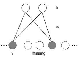
RBM is a two-layer undirected graphical model, see figure 1. It defines a joint distribution over visible variables v and a hidden variable h. In the cold start situation, we consider the case where both v and h are binary vectors.
RBM is an energy-based model, whose energy function is given by
| (1) |
where M is the number of visual units, N is the number of hidden units, are the binary states of visible unit m and hidden unit n, are their biases and is the weight between and . Every joint configuration has probability of the form:
| (2) |
where is the partition function given by summing over all possible configuration of :
| (3) |
For a given visible vector , the marginal probability of is given by
| (4) |
The condition distribution of a visible unit given all the hidden units and the condition distribution of a hidden unit given all the visible units are as follows:
| (5) |
| (6) |
where is the logistic function.
In this paper, each RBM represents a movie, each visual unit represents a user that has rated the movie. This differs from [18] where each RBM represents a user and each visual unit represents a movie. All RBMs have the same number of hidden units and different number of visible units because different movies are rated by different users. The corresponding weights and biases are tied together in all RBMS. So if two movies are rated by the same people, then these two RBM have the same weights and biases. In other words, we could say all movies use the same RBM while the missing value of users that do not rating a specific movie are ignored. This idea is similar to the matrix factorization based technique [11], [15] that only model the observing ratings and ignore the missing values.
3.2 Learning RBM
We need learn the model by adjusting the weights and biases to lower the energy of the item while in the same time arise the energy of other configuration. This could be done by performing the gradient ascent in the log-likelihood of eq. 4,
| (7) |
where T is the number of movies, is the parameter of RBM. The gradient is as follows,
| (8) |
| (9) |
| (10) |
where represents the expectations under the distribution of data and model respectively. is generally easy to get, while cannot be computed in less than exponential time. So we use the Contrastive Divergence (CD) algorithm which is much faster [8]. Instead of , the CD algorithm use , the ’reconstruction’ produced by setting each to 1 with probability in equation 5.
Indeed, maximizing the log likelihood of the data is equivalent to minimizing the Kullback-Liebler divergence between the data distribution and the model distribution. CD only minimizing the data distribution and the reconstruction distribution, and usually the one step reconstruction works well [18]. The update rule is as follows.
| (11) |
| (12) |
| (13) |
where represent the one step reconstruction, is the learning rate.
3.3 Conditional Restricted Boltzmann Machines (CRBMs)
The above model could be used in collaborative filtering as in [18]. But it becomes invalid for new items as there are no rating and the correspond hidden units could not be activated. We must add extra information to this model for solving cold start problem. Conditional RBM (CRBM) could easily take these extra information into account [24], [25].
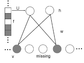
For each movie we use a binary vector to denote its feature and then add directed connection from to its hidden factors . So the joint distribution over conditional on is defined, see figure 2. The energy function becomes the following form.
| (14) |
The conditional distinction of given hidden units is just the same as eq.5. The conditional distribution of becomes the following form.
| (15) |
In CRBM, the hidden states are affected by the feature vector . When we have new items, there are no rating by users, but the hidden state could still be activated by , then the visible unit could be reconstructed as the usual RBM. What’s more, this does not add much extra computation.
Learning the weight matrix U is just like learning the bias of hidden unit. In our experiments, we add an regularization term to the normal gradient known as weight-decay [7]. We used the ’’ penalty function to avoid large weights. The update rule becomes follows.
| (16) |
Weight-decay for U brings some advantages. On one hand, it improves the performance of CRBM by avoid overfitting in the train process. On the other hand, small weight can be more interpretable than very large values which will be shown in section 4. More reasons for weight-decay could be found in [7].
4 Experiment
4.1 DataSet
We illustrate the results on benchmark datasets (MovieLens-100K). In this dataset, there are 100K ratings between 943 users and 1,682 movies. As we mainly focus on the new item cold start problem, we use the items features only (actors and genres). We randomly split the items into two sets. In the test set there are 333 movies which do not appear in the train set to used for cold start. The dataset set comes from the GroupLens project and the items’ feature are downloaded from the Internet Movie Database (http://www.imdb.com).
4.2 Recommendation Task
In this section, we make a distinguish among different recommendation task in real world applications. There are mainly three recommendation tasks depending on the data we have. They are one-class explicit prediction, one-class implicit prediction, and rating prediction.
-
1.
One-class explicit prediction
This task is usually arised where we have data that only contains explict possitive feedback. Our goal is to predict whether a user likes an item or not. In this paper, we convert the original integer rating values from 1 to 5 into binary state 0 and 1. Concretely, if a rating is bigger than 3, we take it as 1, otherwise we take it as 0. As a result, all the rating not bigger than 3 or missing rating are taken to be 0. -
2.
One-class implicit prediction
Implicit rating means some feedback of a user which does not give explicit preference, e.g. the purchase history, watching habits and browsing activity etc. In this task we would predict probability that a user will rate a given movie. In this paper, all the observed ratings are taken to be 1 and all the missing rating are taken to be 0. -
3.
Rating prediction
Rating imputation is to predict whether a user will like an item or not condition on his implicit rating. Usually this could be used to evaluate an algorithm’s performance by holding out some rating from training data and then predicting their ratings. In the train phase, all missing value are ignored and only the observed value are used. In the test phase, only the observed value in the test set are evaluated. This is very different from the former two taskes where all missing value are taken to be 0.
In the first two recommendation taskes all the missing values are taken to be zeros. As a result, the rating matrix becomes dense. While in the rating prediction task, rating matrix could remain sparse. [19] also give three recommendation task which are similar to ours. It’s important to make such a distinction as models can give notable different performance in difference task. In this paper we compare algorithms on these tasks and analysis their performance.
4.3 Evaluation Metrics
Precision-recall curve and root mean square error (RMSE) are two popular evaluation metrics. But both of them may be pitfall when the data class has skew distribution. As we know, the rating data is usually sparse and each user only rates a very small fraction of all the items. A trivial idea is that we take all the pair as 0, then we will get a not very bad result according RMSE or precision-recall curve. Besides they also suffer from the problem of zero rating’s uncertain. Zero rating’s uncertain here means that a missing rating may either indicate the user does not like the item or that the user does not know the item at all.
In this paper, we use receiver operating characteristics (ROC) graph to evaluate the performance of different models. ROC graphs have long been used for organizing classifiers and visualizing their performance. One attractive property of ROC curve is that they are insensitive to changes in class distribution. We could also reduce ROC performance to a single scalar value to compare classifiers, that is the area under the ROC curve (AUC) [3].
4.4 Baselines
In this paper, we mainly focus on the cold start problem. As there are so many techniques for recommender systems, we select three typical models as our baselines. They are aspect model (AS)[19], tied Boltzmann machine (TBM)[6] and regression-based latent factor model (RLFM) [1]. We select these three models because they belong to discrete latent factor model, continuous latent factor model and undirected graphical models respectively. They represent three directions for sovling cold start problems.
The former two models both of which are latent factor models belong to the directed graphical models. Their difference mainly lie in the type of latent factors. In the aspect model, the latent factor is discrete, so aspect model is a mixture model indeed. RLFM is strongly correlated with SVD style matrix factorization methods where the latent factors are continuous. TBM is another type of model belonging to the undirected graphical model which directly models the relationship between items.
4.5 Result
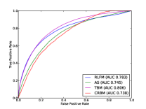
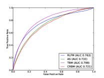
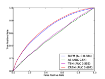
We compare the performance of these four algorithms, including TBM, AS, RLFM and CRBM, in three recommendation tasks, see figure 3. As the one-class implicit prediction and one-class explicit prediction give very similar results, we will use one-class prediction for brief. According to figure 3(a) and figure 3(b), we could sort these models by their performance in descending order and get the result (TBM, RLFM, AS, CRBM). However, we get almost an opposite result when considering figure 3(c). In the following, we discuss how the difference arise. A key difference between one-class prediction and rating prediction is how to deal with the missing value.
On one hand, all user-item pairs have a certain value in the one-class prediction task. All missing value between users and items take value 0 when we train models, see section 4.2. When predicting for cold start items, all user will be considered. The ROC curve is plotted using all pairs between users and new items. On the other hand, we remain the missing state of the corresponding user-item pair. When predicting for new items we only test users that have rated them. The ROC curve is plotted only using user-item pairs in the test set. Concretely, in one-class prediction there are two states for each user-item pair 0 and 1, the rating matrix is a dense. While in rating prediction, the rating matrix is sparse. This difference is of significance and play an important role for evaluate the performance of models. In the former case we need to predict ratings between all user-item pairs. Problems arise when we fill 0 value to the missing pairs which will be illustrated by the following example.
Suppose there are 1000 users and 1000 movies in our data set. Without loss of generality, suppose a user in the test set likes 20 movies. Now we need evaluate an algorithm using this data set. In the one-class prediction task a perfect model should put these 20 movies on the top of the prediction rank list, which means we assume this user like these 20 movies better than other movies. This assumption does not seem rational. It’s very likely that the user likes the other movie better than these 20 ones. Putting these 20 ones in the top rank list is not what we really want to do. We want to know the correct rank of all 1000 movies, but this is impossible generally as the other 900 movies rating are missing. So the problem of rating prediction we caused by its filling missing value.
When comes to the rating prediction, the situation is difference. We only need predict whether a user will like or not for each of the test movie which are all given in the test set. In other words, we just to give a rank list of the test set but not the whole movie set. When we do not know the correct the answer, it’s better to ignore them than to take them as 0. In the above, we analysis the main problem of rating prediction. We must realize that we could not ignore the missing in one-class prediction task just as in rating prediction. Rating prediction could not replace one-class prediction completely because the later is suitable when there are only posititve feedback and no negative feedback. Collaborative filtering techniques, such as use-based CF, item-based CF or matrix factorization, become invalid in such situation. These techniques always give some trivial result, all user liking all items.
It’s easy for us to understand the performance of these four models as we know about the difference and characteristic about the recommendation task. Our data set contains both possitive feedback and negative feedback. So we should use the rating prediction task to evaluate the performance. Though AS model and TBM gives perfect resutls in one-class prediction, they predict ratings in the dense way. They use missing values which includes uncertainty. RFLM and CRBM could deal with the origin sparse raing matrix. If we also sample some negative feedback from the missing pair, they could give good performance in the one-class prediction. In our experiment we sample the negative feedback about 10 times the possitive sapmle.
In the one-class prediction, we ignore the negative feedback and use fewer information both in train and test phase. RFLM and CRBM could deal with this situation. But in the opposite, AS and TBM could only deal with one-class problem, when we ignore the negative feedback in the train phase and predict more informative result, they become invalid, just as the performance of AS and TBM in rating prediction.
4.6 Interpretation
In this section, we will show the matrix U we have learned indeed make sense. The matrix U gives us more intuition. Every row of U could be seen as a feature of movies. A movie has a feature if the feature’s corresponding state is active. Every column could be seen as the correspondence value of actor or genre. So every movie has a representation by actors. If two actors are similar (similar means user has similar rating for movies of these actors), then the value of the distance of correspond column should be small. So we could cluster the actors by U. In this paper we use the k-mean algorithm to cluster the actors. Table 1 illustrates 8 clusters from our experiment. In each cluster, we show 4 actors or genres. we could see who and who are more similary with each other and in which type of movie one actor is usually appear. For example, we see Brad Pitt and Kevin Bacon are more likely appear in the same type movie. Also, the main movie types comedy, crime, war etc. are partitioned into different clusters.
| Topic Number | Actors and Genres |
|---|---|
| 1 | Rance Howard,Parker Posey,James Earl Jones,John Cusack |
| 2 | Children’s, Brad Pitt, Kevin Bacon, Western |
| 3 | Comedy, Paul Herman, Michael Rapaport, John Diehl |
| 4 | R. Lee Ermey, Tim Roth, Dermot Mulroney, War |
| 5 | Wallace Shawn, James Gandolfini, Crime, Sci-Fi |
| 6 | Action, Bruce Willis, Sigourney Weaver, Xander Berkeley |
| 7 | Adventure, Drama, John Travolta, David Paymer |
| 8 | Thriller, Paul Calderon, Gene Hackman, Steve Buscemi |
5 Conclusion and Future work
In this paper, we apply CRBM to solve the new items cold-start problem. In fact, it could be easily extended for new user situation. We compare CRBM with other three typical techniques and show that in the implicit rating prediction and rating prediction task, CRBM gives comparable performance, while in the rating imputation task CRBM gives the best result. According our analysis, the rating imputation task is more coincidence with the real situation. So CRBM shows its superiority to other models. Such results give us more indication for future researches. Firstly, RBM-based models are good at extract features, so we could give more easy explainable result. Secondly, this kinds of model are easily to be applied for online application. When there are new items, we just need update the parameters by the reconstruction. Thirdly, RBM-based model could be easily combined with deep models to extract more feature for recommendation [21].
Just as [27], we do not want to show CRBM models are more superior than the directed graphical models. But the energy-based model give us some more information in different application. In the future we will use deep models to solve the cold start problem.
References
- [1] Deepak Agarwal and Bee-Chung Chen. Regression-based latent factor models. In Proceedings of the 15th ACM SIGKDD International Conference on Knowledge Discovery and Data Mining, pages 19–28. ACM, 2009.
- [2] David M Blei, Andrew Y Ng, and Michael I Jordan. Latent dirichlet allocation. the Journal of Machine Learning Research, 3:993–1022, 2003.
- [3] Tom Fawcett. An introduction to roc analysis. Pattern recognition letters, 27(8):861–874, 2006.
- [4] Zeno Gantner, Lucas Drumond, Christoph Freudenthaler, Steffen Rendle, and Lars Schmidt-Thieme. Learning attribute-to-feature mappings for cold-start recommendations. In International Conference on Data Mining, pages 176–185. IEEE, 2010.
- [5] Peter V Gehler, Alex D Holub, and Max Welling. The rate adapting poisson model for information retrieval and object recognition. In Proceedings of the 23rd International Conference on Machine learning, pages 337–344. ACM, 2006.
- [6] Asela Gunawardana and Christopher Meek. Tied boltzmann machines for cold start recommendations. In Proceedings of the 2008 ACM conference on Recommender Systems, pages 19–26. ACM, 2008.
- [7] Geoffrey Hinton. A practical guide to training restricted boltzmann machines. Momentum, 9(1):926, 2010.
- [8] Geoffrey E Hinton. Training products of experts by minimizing contrastive divergence. Neural Computation, 14(8):1771–1800, 2002.
- [9] Geoffrey E Hinton. To recognize shapes, first learn to generate images. Progress in brain research, 165:535–547, 2007.
- [10] Thomas Hofmann. Probabilistic latent semantic indexing. In Proceedings of the 22nd annual International ACM SIGIR Conference on Research and Development in Information Retrieval, pages 50–57. ACM, 1999.
- [11] Yehuda Koren. Factorization meets the neighborhood: a multifaceted collaborative filtering model. In Proceedings of the 14th ACM SIGKDD international conference on Knowledge discovery and data mining, pages 426–434. ACM, 2008.
- [12] Yehuda Koren, Robert Bell, and Chris Volinsky. Matrix factorization techniques for recommender systems. Computer, 42(8):30–37, 2009.
- [13] Hugo Larochelle and Yoshua Bengio. Classification using discriminative restricted boltzmann machines. In Proceedings of the 25th International Conference on Machine learning, pages 536–543. ACM, 2008.
- [14] Jovian Lin, Kazunari Sugiyama, Min-Yen Kan, and Tat-Seng Chua. Addressing cold-start in app recommendation: latent user models constructed from twitter followers. In Proceedings of the 36th international ACM SIGIR Conference on Research and Development in Information Retrieval, pages 283–292. ACM, 2013.
- [15] Andriy Mnih and Ruslan Salakhutdinov. Probabilistic matrix factorization. In Advances in Neural Information Processing Systems, pages 1257–1264, 2007.
- [16] Seung-Taek Park and Wei Chu. Pairwise preference regression for cold-start recommendation. In Proceedings of the third ACM Conference on Recommender Systems, pages 21–28. ACM, 2009.
- [17] Ruslan Salakhutdinov and Andriy Mnih. Bayesian probabilistic matrix factorization using markov chain monte carlo. In Proceedings of the 25th International Conference on Machine learning, pages 880–887. ACM, 2008.
- [18] Ruslan Salakhutdinov, Andriy Mnih, and Geoffrey Hinton. Restricted boltzmann machines for collaborative filtering. In Proceedings of the 24th International Conference on Machine learning, pages 791–798. ACM, 2007.
- [19] Andrew I Schein, Alexandrin Popescul, Lyle H Ungar, and David M Pennock. Methods and metrics for cold-start recommendations. In Proceedings of the 25th annual International ACM SIGIR Conference on Research and Development in Information Retrieval, pages 253–260. ACM, 2002.
- [20] Paul Smolensky. Information processing in dynamical systems: Foundations of harmony theory. 1986.
- [21] Nitish Srivastava, Ruslan R Salakhutdinov, and Geoffrey E Hinton. Modeling documents with deep boltzmann machines. arXiv preprint arXiv:1309.6865, 2013.
- [22] Xiaoyuan Su and Taghi M Khoshgoftaar. A survey of collaborative filtering techniques. Advances in Artificial Intelligence, page 4, 2009.
- [23] Mingxuan Sun, Fuxin Li, Joonseok Lee, Ke Zhou, Guy Lebanon, and Hongyuan Zha. Learning multiple-question decision trees for cold-start recommendation. In Proceedings of the Sixth ACM International Conference on Web Search and Data Mining, WSDM ’13, pages 445–454, New York, NY, USA, 2013. ACM.
- [24] Ilya Sutskever and Geoffrey E Hinton. Learning multilevel distributed representations for high-dimensional sequences. In International Conference on Artificial Intelligence and Statistics, pages 548–555, 2007.
- [25] Graham W Taylor, Geoffrey E Hinton, and Sam T Roweis. Modeling human motion using binary latent variables. Advances in Neural Information Processing Systems, 19:1345, 2007.
- [26] Chong Wang and David M Blei. Collaborative topic modeling for recommending scientific articles. In Proceedings of the 17th ACM SIGKDD International Conference on Knowledge Discovery and Data Mining, pages 448–456. ACM, 2011.
- [27] Max Welling, Michal Rosen-Zvi, and Geoffrey E Hinton. Exponential family harmoniums with an application to information retrieval. In Advances in Neural Information Processing Systems, volume 17, pages 1481–1488, 2004.
- [28] Mi Zhang, Jie Tang, Xuchen Zhang, and Xiangyang Xue. Addressing cold start in recommender systems: A semi-supervised co-training algorithm. In Proceedings of the 30th Annual International ACM SIGIR Conference on Research and Development in Information Retrieval, 2014.