Quantum discord and measurement-induced disturbance in the background of dilaton black holes

Abstract

We study the dynamics of classical correlation, quantum discord and measurement-induced disturbance of Dirac fields in the background of a dilaton black hole. We present an alternative physical interpretation of single mode approximation for Dirac fields in black hole spacetimes. We show that the classical and quantum correlations are degraded as the increase of black hole’s dilaton. We find that, comparing to the inertial systems, the quantum correlation measured by the one-side measuring discord is always not symmetric with respect to the measured subsystems, while the measurement-induced disturbance is symmetric. The symmetry of classical correlation and quantum discord is influenced by gravitation produced by the dilaton of the black hole.

I introduction

Relativistic quantum information Peres , which is the combination of general relativity, quantum field theory and quantum information, has been a focus of research for both conceptual and experimental reasons. Understanding quantum effects in a relativistic framework is ultimately necessary because the world is essentially noninertial. Also, quantum correlation plays a prominent role in the study of the thermodynamics and information loss problem Bombelli-Callen ; Hawking-Terashima of black holes. It is of a great interest to study how the relativistic effects influence the properties of entanglement, classical correlation, quantum discord, quantum nonlocality, as well as Fisher information Schuller-Mann ; Alsing-Milburn ; jieci3 ; jieci4 ; Ralph ; RQI6 ; adesso2 ; RQI3 ; RQI4 ; RQI5 ; RQI7 in the last few years. Recently, exotic classes of black holes derived from the string theory, i.e., the dilaton black holes Horowitz ; Anabalon ; Amarilla formed by gravitational systems coupled to Maxwell and dilaton fields, have attracted much attention. It is widely believed that the study of dilaton black holes may lead to a deeper understanding of quantum gravity because it emerges from several fundamental theories, such as string theory, black hole physics, and loop quantum gravity.

On the other hand, quantum correlation measured by discord zurek ; Maziero2 ; datta-onequbit ; experimental-onequbit is regarded as a valuable resource for quantum computation and communication in some situations. To calculate the discord of a bipartite state, one makes a one-side measurement on a subsystem $A$ of $\rho_{AB}$ by a complete set of projectors $\{{\Pi^{A}_{j}}\}$ which yields $\rho_{B|j}={Tr_{A}(\Pi^{A}_{j}\rho_{AB}\Pi^{A}_{j})}/{p_{j}}$ with $p_{j}=Tr_{AB}(\Pi^{A}_{j}\rho_{AB}\Pi^{A}_{j})$. The mutual information RAM of $\rho_{AB}$ can alternatively be defined by ${\cal J}_{\{\Pi^{A}_{j}\}}(A:B)=S(\rho_{B})-S_{\{\Pi^{A}_{j}\}}(B|A),$ where $S_{\{\Pi^{A}_{j}\}}(B|A)=\sum_{j}p_{j}S(\rho_{B|j})$ is conditional entropy Cerf of the state. This quantity strongly depends on the choice of the measurements $\{\Pi^{A}_{j}\}$. One should minimize the conditional entropy over all possible measurements on $A$ which corresponds to finding the measurement that disturbs least the overall quantum state zurek . The quantum discord between parts $A$ and $B$ has the form ${\cal D}(A:B)={\cal I}(A:B)-{\cal C}(A:B)$, where ${\cal C}(A:B)$ is the classical correlation ${\cal C}(A:B)=\max_{\{\Pi^{A}_{j}\}}{\cal J}_{\{\Pi^{A}_{j}\}}(A:B)$ and ${\cal I}(A:B)$ is the quantum mutual information quantifying the total correlation. So quantum discord describes the discrepancy between total correlation and classical correlation, and it thus provides a measure of quantumness of correlations. In most situations of inertial systems, the quantum discord is symmetric with respect to the subsystem to be measured zurek ; Maziero2 ; Horodecki2 . However, is the symmetry still tenable in the noninertial systems, especially in the curved spacetimes? Besides, does the spacetime background also affects the quantum correlations by some other measures such as the measurement-induced disturbance (MID)?

In this paper we discuss the properties of classical correlation, quantum discord and MID Maziero3 for free modes in the background of a dilaton black hole Horowitz . The study of relativistic quantum information on accelerated free modes has its own advantages other than that of local modes RQI5 ; RQI6 in the understanding of quantum effects in curved spacetimes in the sense that there are no proved feasible localized detector models inside the event horizon of a black hole. We assume that two observers, Alice and Bob, measure their local state respectively. After sharing an entangled initial state, Alice stays stationary at an asymptotically flat region, while Bob moves with uniform acceleration and hovers near the event horizon of the dilaton black hole. We calculate the classical correlation and quantum discord by making one-side measurements on a subsystem of the bipartite system, and then get the MID measurement correlations by measuring both of the two subsystems. We are interested in how the dilaton charge will influence the classical correlation, quantum discord, and MID, as well as if these correlations are symmetric under the effect of gravitation produced by the dilaton of the black hole.

The paper is organized as follows. In the next section we discuss the quantization of Dirac fields in the background of the dilaton black hole beyond single mode approximation Bruschi ; Bruschi1 . In Sec. III we study the properties of classical correlation, quantum discord, and MID for Dirac fields in the dilaton spacetime. We will summarize and discuss our conclusions in the last section.

II Quantization of Dirac fields in dilaton black hole spacetimes

The massless Dirac equation in a general background spacetime can be written as Brill

$$[\gamma^{a}e_{a}{}^{\mu}(\partial_{\mu}+\Gamma_{\mu})]\Psi=0,$$ (1)

where $\gamma^{a}$ are the Dirac matrices, the four-vectors $e_{a}{}^{\mu}$ represent the inverse of the tetrad $e^{a}{}_{\mu}$ defined by $g_{\mu\nu}=\eta_{ab}e^{a}{}_{\mu}e^{b}{}_{\nu}$ with $\eta_{ab}={\rm diag}(-1,1,1,1)$, $\Gamma_{\mu}=\frac{1}{8}[\gamma^{a},\gamma^{b}]e_{a}{}^{\nu}e_{b\nu;\mu}$ are the spin connection coefficients.

The metric for a Garfinkle-Horowitz-Strominger dilaton black hole spacetime can be expressed as Horowitz

$$ds^{2}= - \left(\frac{r-2M}{r-2\alpha}\right)dt^{2}+\left(\frac{r-2M}{r-2\alpha}\right)^{-1}dr^{2}$$ (2)

$$+ r(r-2\alpha)d\Omega^{2},$$

where $M$ and $\alpha$ are the mass of the black hole and the dilaton. Throughout this paper we set $G=c=\hbar=\kappa_{B}=1$. This black hole has two singular points at $r=2M$ and $r=2\alpha$. Besides, the dilaton $\alpha$ and the mass $M$ of the black hole should satisfy $\alpha<M$. In order to separate the Dirac equation, we adopt a tetrad as

$$e^{a}{}_{\mu}=diag\bigg{(}\sqrt{f},\frac{1}{\sqrt{f}},\sqrt{r\tilde{r}},\sqrt{r\tilde{r}}\sin\theta\bigg{)},$$ (3)

where $f=(r-2M)/\tilde{r}$ and $\tilde{r}=r-2\alpha$. Then Eq. (1) in the Garfinkle-Horowitz-Strominger dilaton black-hole spacetime becomes

$$- \frac{\gamma_{0}}{\sqrt{f}}\frac{\partial\Psi}{\partial t}+\sqrt{f}\gamma_{1}\left[\frac{\partial}{\partial r}+\frac{r-\alpha}{r\tilde{r}}+\frac{1}{4f}\frac{df}{dr}\right]\Psi$$

$$+ \frac{\gamma_{2}}{\sqrt{r\tilde{r}}}(\frac{\partial}{\partial\theta}+\frac{1}{2}\cot\theta)\Psi$$

$$+ \frac{\gamma_{3}}{\sqrt{r\tilde{r}}\sin\theta}\frac{\partial\Psi}{\partial\varphi}=0.$$

If we rescale $\Psi$ as $\Psi=f^{-\frac{1}{4}}\Phi$ and use an ansatz for the Dirac spinor similar to Ref. jieci1 , we can solving the Dirac equation near the event horizon. For the outside and inside region of the event horizon, we obtain the positive frequency outgoing solutions D-R ; jieci2

$$\Psi^{+}_{out,\mathbf{k}}=\mathcal{G}e^{-i\omega\mathcal{U}},$$ (6)

$$\Psi^{+}_{in,\mathbf{k}}=\mathcal{G}e^{i\omega\mathcal{U}},$$ (7)

where $\mathcal{U}=t-r_{*}$ and $\mathcal{G}$ is a four-component Dirac spinor, $\mathbf{k}$ is the wavevector we used to label the modes hereafter and for massless Dirac field $\omega=|\mathbf{k}|$. In terms of these basis the Dirac field $\Psi$ can be expanded as

$$\Psi = \int d\mathbf{k}[\hat{a}^{out}_{\mathbf{k}}\Psi^{+}_{out,\mathbf{k}}+\hat{b}^{out{\dagger}}_{\mathbf{-k}}\Psi^{-}_{out,\mathbf{k}}$$ (8)

$$+ \hat{a}^{in}_{\mathbf{k}}\Psi^{+}_{in,\mathbf{k}}+\hat{b}^{in{\dagger}}_{\mathbf{-k}}\Psi^{-}_{in,\mathbf{k}}],$$

where $\hat{a}^{out}_{\mathbf{k}}$ and $\hat{b}^{out{\dagger}}_{\mathbf{k}}$ are the fermion annihilation and antifermion creation operators acting on the state of the exterior region, and $\hat{a}^{in}_{\mathbf{k}}$ and $\hat{b}^{in{\dagger}}_{\mathbf{k}}$ are the fermion annihilation and antifermion creation operators acting on the interior vacuum of the black hole respectively. The annihilation operator $\hat{a}^{out}_{\mathbf{k}}$ and creation operator $\hat{a}^{out}_{\mathbf{k}}$ satisfy the canonical anticommutation $\{\hat{a}^{out}_{\mathbf{k}},\hat{a}^{out}_{\mathbf{k^{\prime}}}\}=\delta_{\mathbf{k}\mathbf{k^{\prime}}}$ and $\{\hat{a}^{out}_{\mathbf{k}},\hat{a}^{out\dagger}_{\mathbf{k^{\prime}}}\}=\{\hat{a}^{out\dagger}_{\mathbf{k}},\hat{a}^{out\dagger}_{\mathbf{k^{\prime}}}\}=0$, where $\{.,.\}$ denotes the anticommutator. Clearly, two fermionic Fock are antisymmetric with respect to the exchange of the mode labels $\mathbf{k}$ and $\mathbf{k^{\prime}}$ due to the anticommutation relations. We therefore define

$$||1_{\mathbf{k}}1_{\mathbf{k^{\prime}}}\rangle\rangle=\hat{a}^{\dagger}_{\mathbf{k}},\hat{b}^{\dagger}_{\mathbf{k^{\prime}}}||0\rangle\rangle=-\hat{b}^{\dagger}_{\mathbf{k^{\prime}}},\hat{a}^{\dagger}_{\mathbf{k}}||0\rangle\rangle,$$ (9)

where the states in the antisymmetric fermionic Fock space are denoted by double-lined Dirac notation $||.\rangle\rangle$ antifermi rather than the single-lined notations.

Making analytic continuation for Eqs. (6) and (7), we find a complete basis for positive energy modes, i.e., the Kruskal modes, according to the suggestion of Domour-Ruffini D-R . Then we can quantize the massless Dirac field in black hole and Kruskal modes respectively jieci1 ; jieci2 , from which we can easily get the Bogoliubov transformations Barnett between the creation and annihilation operators in different coordinates jieci1 . Considering that it is more interesting to quantize the Dirac field beyond the single mode approximation Bruschi ; Bruschi1 . We construct a different set of creation operators that are linear combinations of creation operators in the inside and outside regions Bruschi ; Bruschi1

$$\tilde{c}_{\mathbf{k},R} = \cos r\hat{a}^{out}_{\mathbf{k}}-\sin r\hat{b}^{in\dagger}_{\mathbf{-k}},$$

$$\tilde{c}_{\mathbf{k},L} = \cos r\hat{a}^{in}_{\mathbf{k}}-\sin r\hat{b}^{out\dagger}_{\mathbf{-k}},$$

$$\tilde{c}^{\dagger}_{\mathbf{k},R} = \cos r\hat{a}^{out\dagger}_{\mathbf{k}}-\sin r\hat{b}^{in}_{\mathbf{-k}},$$

$$\tilde{c}^{\dagger}_{\mathbf{k},L} = \cos r\hat{a}^{in\dagger}_{\mathbf{k}}-\sin r\hat{b}^{out}_{\mathbf{-k}},$$ (10)

where $\cos r=[e^{-8\pi\omega(M-\alpha)}+1]^{-\frac{1}{2}}$ and $\sin r=[e^{8\pi\omega(M-\alpha)}+1]^{-\frac{1}{2}}$. We name the modes (or operators) with subscripts L and R by “left” and “right” modes (or operators), respectively. After properly normalizing the state vector, the Kruskal vacuum is found to be $||0\rangle\rangle_{K}=\bigotimes_{\mathbf{k}}||0_{\mathbf{k}}\rangle\rangle_{K}=\bigotimes_{\mathbf{k}}||0_{\mathbf{k}}\rangle\rangle_{R}\otimes||0_{\mathbf{k}}\rangle\rangle_{L}$, where $|||0_{\mathbf{k}}\rangle\rangle_{R}$ and $|||0_{\mathbf{k}}\rangle\rangle_{L}$ are annihilated by the annihilation operators $\tilde{c}_{\mathbf{k},R}$ and $\tilde{c}_{\mathbf{k},L}$. The vacuum state $||0_{\mathbf{k}}\rangle\rangle_{K}$ for mode $\mathbf{k}$ is given by

$$||0_{\mathbf{k}}\rangle\rangle_{K} = \cos^{2}r||0000\rangle\rangle-\sin r||0011\rangle\rangle$$ (11)

$$+ \sin r\cos r||1100\rangle\rangle-\sin^{2}r||1111\rangle\rangle,$$

where $||mnm^{\prime}n^{\prime}\rangle\rangle=||m_{\mathbf{k}}\rangle\rangle^{+}_{out}||n_{-\mathbf{k}}\rangle\rangle^{-}_{in}||m^{\prime}_{-\mathbf{k}}\rangle\rangle^{-}_{out}||n^{\prime}_{\mathbf{k}}\rangle\rangle^{+}_{in}$, $\{||n_{-\mathbf{k}}\rangle\rangle^{-}_{in}\}$ and $\{||n_{\mathbf{k}}\rangle\rangle^{+}_{out}\}$ are the orthonormal bases for the inside and outside region of the dilaton black hole respectively, and the $\{+,-\}$ superscript on the kets is used to indicate the fermion and antifermion vacua. For the observer Bob who travels outside the event horizon, the Hawking radiation spectrum from the view of his detector can be obtained by

$$N_{\omega}^{2}=_{K}\langle 0|\hat{a}^{out{\dagger}}_{\mathbf{k}}\hat{a}^{out}_{\mathbf{k}}|0\rangle_{K}=\frac{1}{e^{\omega/T}+1},$$

where $T=\frac{1}{8\pi(M-\alpha)}$ is Hawking temperature Hawking of the black hole. This equation shows that the observer in the exterior of the Garfinkle-Horowitz-Strominger dilaton black hole detects a thermal Fermi-Dirac distribution of particles. Because of the Pauli exclusion principle, only the first excited state for each fermion mode $||1_{\mathbf{k}}\rangle\rangle^{+}_{K}$ is allowed, and similarly for antifermions. The first excited state for the fermion mode is given by

$$||1_{\mathbf{k}}\rangle\rangle^{+}_{K} =\left[q_{R}(\tilde{c}^{\dagger}_{\mathbf{k},R}\otimes I_{L})+q_{L}(I_{R}\otimes\tilde{c}^{\dagger}_{\mathbf{k},L})\right]||0_{\mathbf{k}}\rangle\rangle_{K}$$ (12)

$$=q_{R}[\cos r||1000\rangle\rangle-\sin r||1011\rangle\rangle]$$

$$+q_{L}[\sin r||1100\rangle\rangle+\cos r||0001\rangle\rangle],$$

with $|q_{R}|^{2}+|q_{L}|^{2}=1$. The study of fermionic quantum information beyond the single mode approximation, which was proposed in Bruschi and widely adopted recently, has a lack of physical interpretation so far. Here we present an alternative physical interpretation on the operators and states that obtained beyond such an approximation in black hole spacetimes. The operator $\tilde{c}^{\dagger}_{\mathbf{k},R}$ in Eq.(II) indicates the creation of two particles, i.e., a fermion in the exterior vacuum and an antifermion in the interior vacuum of the black hole. Similarly, the create operator $\tilde{c}^{\dagger}_{\mathbf{k},L}$ means that an antifermion and an fermion are created outside and inside the event horizon, respectively. Hawking radiation comes from spontaneous creation of paired particles and antiparticles by quantum fluctuations near the event horizon. The particles and antiparticles can radiate toward the inside and outside regions randomly from the event horizon with the total probability $|q_{R}|^{2}+|q_{L}|^{2}=1$. Thus, $|q_{R}|=1$ means that all the particles move toward the black hole exteriors while all the antiparticles move to the inside region, i.e., only particles can be detected as Hawking radiation. Similarly, $|q_{L}|=1$ indicates that only antiparticles escapes from the event horizon. Therefore, the single mode approximation (either $|q_{R}|=1$ or $|q_{L}|=1$) is a special case when either only particles or only antiparticles are detected.

III Quantum discord and MID in dilaton black hole spacetimes

We assume that Alice and Bob share a maximally entangled state

$$||\Phi\rangle\rangle_{AB}=\frac{1}{\sqrt{2}}(||0\rangle\rangle_{A}||0\rangle\rangle_{B}+||1\rangle\rangle^{+}_{A}||1\rangle\rangle^{+}_{B}),$$ (13)

at the same point in the asymptotically flat region of the dilaton black hole. Then Alice stays stationary at the asymptotically flat region, while Bob moves with uniform acceleration and hovers near the event horizon of the dilaton black hole. Bob will detects a thermal Fermi-Dirac distribution of particles and his detector is found to be excited. Using Eqs. (11) and (12), we can rewrite Eq. (13). Since Bob is causally disconnected from the region inside the event horizon we should trace over the state of the inside region and obtain

$$\varrho^{AB_{out}} = \frac{1}{2}\Big{[}C^{4}\left||{000}\right\rangle\rangle\left\langle\langle{000}\right||+S^{2}C^{2}(\left||{010}\right\rangle\rangle\left\langle\langle{010}\right||$$ (14)

$$+ \left||{001}\right\rangle\rangle\left\langle\langle{001}\right||)+\phantom{\Big{[}}S^{4}\left||{011}\right\rangle\rangle\left\langle\langle{011}\right||$$

$$+ |q_{\text{\text{R}}}|^{2}(C^{2}\left||{110}\right\rangle\rangle\left\langle\langle{110}\right||+S^{2}\left||{111}\right\rangle\rangle\left\langle\langle{111}\right||)$$

$$+ \phantom{\Big{[}}|q_{\text{\text{L}}}|^{2}(S^{2}\!\left||{110}\right\rangle\rangle\left\langle\langle{110}\right||\!+\!C^{2}\!\left||{100}\right\rangle\rangle\left\langle\langle{100}\right||)$$

$$+ q_{\text{\text{R}}}^{*}(C^{3}\!\left||{000}\right\rangle\rangle\left\langle\langle{110}\right||+S^{2}C\left||{001}\right\rangle\rangle\left\langle\langle{111}\right||)$$

$$- q_{\text{\text{L}}}^{*}(C^{2}S\!\left||{001}\right\rangle\rangle\left\langle\langle{100}\right||+S^{3}\!\left||{011}\right\rangle\rangle\left\langle\langle{110}\right||)$$

$$\!\!-q_{\text{R}}q_{\text{L}}^{*}SC\!\left||{111}\right\rangle\rangle\left\langle\langle{100}\right||\Big{]}+(\text{H.c.})_{{}_{\begin{subarray}{c}\text{non-}\text{diag.}\end{subarray}}}$$

where $||lmn\rangle\rangle=||l\rangle\rangle_{A}||m_{\mathbf{k}}\rangle\rangle^{+}_{out}||n_{\mathbf{-k}}\rangle\rangle^{-}_{out}$, $S=\sin r$ and $C=\cos r$. We assume that Bob has a detector sensitive only to the particle modes, which means that an antifermion cannot be excited in a single detector when a fermion was detected. Thus, we should also trace out the antifermion mode $||n_{\mathbf{-k}}\rangle\rangle^{-}_{out}$ in the outside region Bruschi1

$$\varrho^{A\tilde{B}} = \frac{1}{2}\bigg{[}C^{2}||00\rangle\rangle\langle\langle 00|+q^{*}_{\text{R}}C||00\rangle\rangle\langle\langle 11||$$ (15)

$$+ q_{\text{R}}C||11\rangle\rangle\langle\langle 00||)+q_{\text{L}}C^{2}||10\rangle\rangle\langle\langle 10||$$

$$+ S^{2}||01\rangle\rangle\langle\langle 01||+\chi_{0}||11\rangle\rangle\langle\langle 11||\bigg{]},$$

where $||lm\rangle\rangle=||l\rangle\rangle_{A}||m_{\mathbf{k}}\rangle\rangle^{+}_{out}$ and $\chi_{0}=|q_{\text{R}}|^{2}+|q_{\text{L}}|^{2}S^{2}$. Hereafter we call the mode $\||m_{\mathbf{k}}\rangle\rangle^{+}_{out}$ as $\tilde{B}$. Now our system has two subsystems, i.e., the inertial subsystem $A$ and accelerated subsystem $\tilde{B}$. We can easily obtain the von Neumann entropy $S(\rho_{A,\tilde{B}})$ of this state, $S(\rho_{A})$ for the reduced density matrix of the mode $A$ and $S(\rho_{\tilde{B}})$ for the mode $\tilde{B}$, respectively.

III.1 Measurements on subsystem $A$

Now let us first make measurements on the subsystem $A$, the projectors are defined as zurek ; datta-onequbit ; jieci3

$$\Pi^{A}_{+}=\frac{I_{2}+\mathbf{n}\cdot\mathbf{\sigma}}{2}\otimes I_{2},\ \ \ \ \ \Pi^{A}_{-}=\frac{I_{2}-\mathbf{n}\cdot\mathbf{\sigma}}{2}\otimes I_{2},$$ (16)

where $n_{1}=\sin\theta\cos\varphi,\ n_{2}=\sin\theta\sin\varphi,\ n_{3}=\cos\theta$ and $\sigma_{i}$ are Pauli matrices. The measurement operators in Eq. (16) include a two-outcome projective measurement operator $\frac{I_{2}\pm\mathbf{n}\cdot\mathbf{\sigma}}{2}$ on subsystem $A$ and an identity operator on subsystem $B$. These operators are orthogonal projectors spanning the qubit Hilbert space and can therefore be parameterized by the unit vector $\mathbf{n}=(n_{1},n_{2},n_{3})$. For simplicity, here we can take the measurements on the particle-number degree of freedom, i.e., to measure whether or not a fermion with wave vector $\mathbf{k}$ is excited in the particle detector. After the measurement of $\Pi^{A}_{+}$, the quantum state $\rho_{A,\tilde{B}}$ changes to

$$\rho^{MA}_{+} = Tr_{A}(\Pi^{A}_{+}\rho_{A,\tilde{B}}\Pi^{A}_{+})/p^{A}_{+}$$ (19)

$$= \frac{1}{2}\left[\begin{array}[]{cc}\varsigma_{1}&e^{i\varphi}q^{*}_{\text{R}}C\sin\theta\\ e^{-i\varphi}q_{\text{R}}C\sin\theta&\chi_{1}\\ \end{array}\right],$$

where $p^{A}_{+}=Tr(\Pi^{A}_{+}\rho_{A,\tilde{B}}\Pi^{A}_{+})=1/2$, $\varsigma_{1}=C^{2}[1+\cos\theta+q_{\text{L}}(1-\cos\theta)]$ and $\chi_{1}=\chi_{0}(1-\cos\theta)+(1+\cos\theta)S^{2}$. The same method is used to compute the state after measurement $\Pi^{A}_{-}$, then we have

$$\rho^{MA}_{-}=\frac{1}{4p^{A}_{-}}\left[\begin{array}[]{cc}\varsigma_{2}&-e^{i\varphi}q^{*}_{\text{R}}C\sin\theta\\ -e^{-i\varphi}q_{\text{R}}C\sin\theta&\chi_{2}\\ \end{array}\right],$$ (22)

where $p^{A}_{-}=Tr(\Pi^{A}_{-}\rho_{A,\tilde{B}}\Pi^{A}_{-})=1/2$, $\varsigma_{2}=C^{2}[1-\cos\theta+q_{\text{L}}(1+\cos\theta)]$ and $\chi_{2}=\chi_{0}(1+\cos\theta)+(1-\cos\theta)S^{2}$. Now we can obtain the conditional entropy $S_{\{\Pi^{A}_{j}\}}(\tilde{B}|A)\equiv\sum_{j}p_{j}S(\tilde{B}|j)$. The classical correlation in this case is

$${\cal C}(\tilde{B}|A)=S(\rho_{\tilde{B}})-\min_{\Pi^{A}_{j}}S_{\{\Pi^{A}_{j}\}}(\tilde{B}|A),$$

and the quantum discord is

$${\cal D}(\tilde{B}|A)=S(\rho_{\tilde{A}})-S(\rho_{A,\tilde{B}})+\min_{\Pi^{A}_{j}}S_{\{\Pi^{A}_{j}\}}(\tilde{B}|A).$$

Note that the conditional entropy has to be numerically evaluated by optimizing over the angles $\theta$ and $\phi$. Thus we should minimize it over all possible measurements on $A$ zurek . We find that the condition entropy is independent of $\varphi$ and its minimum can be obtained when $\theta=\pi/2$.

III.2 Measurements on subsystem ${\tilde{B}}$

Then let us make our measurements on the subsystem ${\tilde{B}}$; the projectors are defined as

$$\Pi^{\tilde{B}}_{+}=I_{2}\otimes\frac{I_{2}+\mathbf{n}\cdot\sigma}{2},\ \ \ \ \ \Pi^{\tilde{B}}_{-}=I_{2}\otimes\frac{I_{2}-\mathbf{n}\cdot\sigma}{2}.$$ (23)

After the measurement of $\Pi^{\tilde{B}}_{+}$, the state $\rho_{A,\tilde{B}}$ changes to

$$\rho^{M\tilde{B}}_{+}=\frac{1}{4p^{\tilde{B}}_{+}}\left[\begin{array}[]{cc}\varsigma_{3}&~{}~{}~{}~{}e^{i\varphi}q^{*}_{\text{R}}\sin r\sin\theta\\ e^{-i\varphi}q_{\text{R}}\sin r\sin\theta&\chi_{3}\\ \end{array}\right],$$ (26)

where $p^{\tilde{B}}_{+}=(1-\cos 2r\cos\theta)(1+q^{2}_{\text{L}})+q^{2}_{\text{R}}(1+\cos\theta)$, $\varsigma_{3}=(1+\cos\theta)C^{2}+(1-\cos\theta)S^{2}$ and $\chi_{3}=q^{2}_{\text{L}}C^{2}(1-\cos\theta)+\chi_{0}(1+\cos\theta)$. Similarly, we can calculate the state after $\Pi^{\tilde{B}}_{-}$ and get the classical correlation ${\cal C}(A|\tilde{B})$ and the quantum discord ${\cal D}(A|\tilde{B})$ respectively.

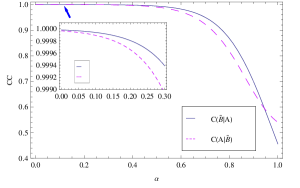
Figure 1: (Color online) The classical correlation ${\cal C}(\tilde{B}|A)$ obtained by measuring the subsystem $A$ and the classical correlation ${\cal C}(A|\tilde{B})$ (dashed line) as a function of the dilaton$\alpha$. We set $M=\omega=1$ and $q_{R}=1$.

Figure 1 shows how the dilaton $\alpha$ of the black hole influences the classical correlations of the system when we obtain them by measuring the subsystem $A$ and ${\tilde{B}}$, respectively. From which we can see that for all the two cases the classical correlations decrease with increasing dilaton $\alpha$. The classical correlation ${\cal C}(\tilde{B}|A)$ obtained by the one-side measurements on subsystem $A$, is always not equal to ${\cal C}(A|\tilde{B})$ for any dilaton value. In contrast, the classical correlations satisfy ${\cal C}(B|A)={\cal C}(A|B)=1$ for the initial state, Eq.(13), in the asymptotically flat region. Comparing to the flat spacetime, the classical correlation (of course the related quantum correlation) is not symmetrical in the dilaton black hole spacetime. This asymmetry is due to the effect of gravitation produced by the black hole. We also note that ${\cal C}(\tilde{B}|A)$ is larger than ${\cal C}(A|\tilde{B})$ when the dilaton is smaller than a fixed value ($\alpha\simeq 0.9451$), while it is smaller than ${\cal C}(A|\tilde{B})$ when the dilaton is larger than this value.

III.3 Symmetric measurement of the correlations

From the foregoing discussion, we see that the classical and quantum correlations in the curved spacetime depend on the measurement process. At the same time, a symmetric measurement of the quantum correlation was proposed recently. The MID measurement Maziero3 , which is obtained by a complete set of projective measurements over both partitions of a bipartite state, is given by  Maziero3

$${\cal D}(MID)=\mathcal{I}(\rho_{A,\tilde{B}})-\mathcal{I}(\eta_{A,\tilde{B}})$$ (27)

with

$$\eta_{A,\tilde{B}}=\sum_{i=1}^{m}\sum_{j=1}^{n}\mathbf{\pi}_{i}^{A}\otimes\mathbf{\pi}_{j}^{\tilde{B}}\rho_{A,\tilde{B}}\mathbf{\pi}_{i}^{A}\otimes\mathbf{\pi}_{j}^{\tilde{B}}.$$ (28)

where $\mathbf{\pi}_{i}^{A}=||i\rangle\rangle\langle\langle i||$ and $\mathbf{\pi}_{j}^{\tilde{B}}=||j\rangle\rangle\langle\langle j||$ are one-dimensional orthogonal projections for parties $A$ and $\tilde{B}$, respectively. Such a symmetrized version of the quantum correlation was recently discussed theoretically  Maziero3 and experimentally measured by anuclear magnetic resonance setup at room temperature NMR . Besides, MID requires only the local measurement strategy rather than the cumbersome optimization required by the derivation of discord Rao . Here we can easily obtain $\eta_{A,\tilde{B}}$ and find the MID measure of classical correlation ${\cal C}(MID)$ and quantum correlation ${\cal D}(MID)$.

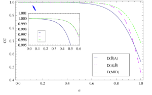
Figure 2: (Color online) The quantum discord ${\cal D}(\tilde{B}|A)$(solid line), ${\cal D}(A|\tilde{B})$ (dashed line), and ${\cal D}(MID)$ (dotted line) of $\rho_{A,\tilde{B}}$ as a function of the dilaton $\alpha$. We set $M=\omega=1$ and $q_{R}=1$.

Figure 2 shows how the dilaton of the black hole affects the quantum correlations (discord and MID) that obtained by different measuring methods. Both the quantum discord and the MID decrease as the increasing of $\alpha$, which means the quantum correlations degraded as the increase of dilaton $\alpha$. It is shown that the discord ${\cal D}(A|\tilde{B})$ is not equal to ${\cal D}(\tilde{B}|A)$ for any $\alpha$, which is extremely different from ${\cal D}(B|A)={\cal D}(A|B)=1$ in the initial state Eq. (13). Comparing to the flat spacetime, the quantum discord is not symmetric for any $\alpha$ in the dilaton black hole spacetime. The symmetry of quantum discord is truly influenced by the dilaton of the black hole. It is also noted that the quantum correlation obtained via the MID measurement is always larger than that obtained by the one-side measurement.

IV summary

The effect of black hole’s dilaton on the symmetry of classical correlation, quantum discord, and MID for the Dirac fields is investigated. We give a physical interpretation of the single mode approximation in the curved spacetime, i.e., such an approximation is a special case when either only particles or only antiparticles are detected. It is shown that the classical and quantum correlations decrease monotonously as increasing dilaton, which means all type of correlations are degraded due to the effect of gravitation generated by the dilaton of the black hole. We find that both the one-side measured classical and quantum correlations are not symmetric with respect to the subsystem being measured. So both the quantification and the symmetry of classical correlation and quantum discord are influenced by the gravitation when taking the one-side measurement. This is a sharp comparison between the inertial systems and the system in the curved spacetime. The results obtained here are not only helpful to understanding the symmetric properties of classical and quantum correlations in the presence of strong gravitation but also give a better insight into quantum properties of dilaton black holes.

- (1) A. Peres and D. R. Terno, Rev. Mod. Phys. 76, 93 (2004).
- (2) L. Bombelli, R. K. Koul, J. Lee, and R. D. Sorkin, Phys. Rev. D 34, 373 (1986).
- (3) S. W. Hawking, Commun. Math. Phys. 43, 199 (1975); Phys. Rev. D 14, 2460 (1976); H. Terashima, Phys. Rev. D 61, 104016 (2000).
- (4) P. M. Alsing and G. J. Milburn, Phys. Rev. Lett. 91, 180404 (2003).
- (5) I. Fuentes-Schuller and R. B. Mann, Phys. Rev. Lett. 95, 120404 (2005).
- (6) T. C. Ralph, G. J. Milburn, and T. Downes, Phys. Rev. A 79, 022121 (2009); J. Doukas and L. C.L. Hollenberg, Phys. Rev. A 79, 052109 (2009); S. Moradi, Phys. Rev. A 79, 064301 (2009).
- (7) A. Datta, Phys. Rev. A 80, 052304 (2009); J. Wang, J. Deng, and J. Jing, Phys. Rev. A 81, 052120 (2010); E. G. Brown, K. Cormier, E. Martín-Martínez, and R. B. Mann, Phys. Rev. A 86, 032108 (2012).
- (8) J. Wang and J. Jing, Phys. Rev. A 82, 032324 (2010); 83, 022314 (2011).
- (9) M. Aspachs, G. Adesso, and I. Fuentes, Phys. Rev. Lett 105, 151301 (2010).
- (10) S. Khan and M. K. Khan, J. Phys. A 44, 045305, (2011); X. Xiao and M. Fang, J. Phys. A 44, 145306 (2011); M. Z. Piao and X. Ji, J. Mod. Opt., 59, 21 (2012); M. Ramzan, Eur.Phys. J. D 67, 170 (2013).
- (11) J. Feng, Y.-Z. Zhang, M. D. Gould, and H. Fan, Phys. Lett. B 726, 527(2013); D. J. Hosler and P. Kok, Phys. Rev. A 88, 052112. (2013).
- (12) S. Xu, X.-K. Song, J.-D. Shi, and L. Ye, Phys. Rev. D 89,065022 (2014); Y. Yao, X. Xiao, L. Ge, X. G. Wang, and C. P. Sun, Phys. Rev. A 89, 042336 (2014).
- (13) N. Friis, A. R. Lee, D. E. Bruschi, and J. Louko, Phys. Rev. D 85, 025012 (2012); D. E. Bruschi, I. Fuentes, and J. Louko, Phys. Rev. D 85, 061701(R)(2012).
- (14) N. Friis, A. R. Lee, K. Truong, C. Sabín, E. Solano, G. Johansson, and I. Fuentes, Phys. Rev. Lett. 110, 113602 (2013); E. Martín-Martínez, D. Aasen, and A. Kempf, Phys. Rev. Lett. 110, 160501 (2013).
- (15) D. Garfinkle, G. T. Horowitz, and A. Strominger, Phys. Rev. D 43, 3140 (1991); A. Garcia, D. Galtsov and O. Kechkin, Phys. Rev. Lett. 74 1276, (1995); J. Wang, Q. Pan, S. Chen, and J. Jing, Phys. Lett. B 677, 186 (2009).
- (16) L. Nakonieczny and M. Rogatko, Phys. Rev. D 84, 044029 (2011); A. Anabalon, D. Astefanesei, R. Mann, J. High Energy Phys. 10, (2013)184.
- (17) L. Amarilla and E. F. Eiroa, Phys. Rev. D 87, 044057 (2013).
- (18) H. Ollivier and W. H. Zurek, Phys. Rev. Lett. 88, 017901 (2001).
- (19) J. Maziero et al., Phys. Rev. A 81, 022116 (2010).
- (20) A. Datta, A. Shaji, and C. M. Caves, Phys. Rev. Lett. 100, 050502 (2008).
- (21) B. P. Lanyon, M. Barbieri, M. P. Almeida, and A. G. White, Phys. Rev. Lett.101, 200501 (2008).
- (22) R. S. Ingarden, A. Kossakowski, and M. Ohya, Information Dynamics and Open Systems - Classical and Quantum Approach (Kluwer Academic Publishers, Dordrecht, 1997).
- (23) N. J. Cerf and C. Adami, Phys. Rev. Lett. 79, 5194 (1997).
- (24) M. Horodecki et al., Phys. Rev. A 71, 062307 (2005).
- (25) D. P. DiVincenzo et al., Phys. Rev. Lett. 92, 067902 (2004); S. Luo, Phys. Rev. A 77, 022301 (2008); K. Modi et al., Phys. Rev. Lett. 104, 080501 (2010); K. Modi, A. Brodutch, H. Cable, T. Paterek, and V. Vedral Rev.Mod. Phys. 84, 1655 (2012).
- (26) D. E. Bruschi, J. Louko, E. Martín-Martínez, A. Dragan, and I. Fuentes, Phys. Rev. A 82, 042332 (2010).
- (27) N. Friis et al., Phys. Rev. A 84, 062111 (2011); M. Montero, J. Leon, and E. Martín-Martínez, Phys. Rev. A 84, 042320 (2011); J. Chang and Y. Kwon, Phys. Rev. A 85, 032302 (2012).
- (28) D. R. Brill and J. A. Wheeler, Rev. Mod. Phys. 29, 465 (1957); Phys. Rev. D 45, 3888(E) (1992).
- (29) J. Wang, Q. Pan, S. Chen, and J. Jing, Quantum Inf. Comput. 10, 0947 (2010).
- (30) T. Damoar and R. Ruffini, Phys. Rev. D 14, 332 (1976).
- (31) J. Wang, Q. Pan, and J. Jing, Ann. Phys. (New York)325, 1190 (2010); Phys. Lett. B 602, 202 (2010).
- (32) N. Friis, A. R. Lee, and D. E. Bruschi, Phys. Rev. A 87, 022338 (2013).
- (33) S. M. Barnett and P. M. Radmore, Methods in Theoretical Quantum Optics (Oxford University Press, New York, 1997), pp. 67-80.
- (34) S. W. Hawking, Nature(London) 248, 30 (1974); S. A. Haywarda, R. Di Criscienzob, M. Nadalinic, L. Vanzoc, and S. Zerbini, Classcal Quantum Gravity 26, 062001 (2009).
- (35) D. O. Soares-Pinto et al., Phys. Rev. A 81, 062118 (2010).
- (36) B. R. Rao, R. Srikanth, C. M. Chandrashekar, and S. Banerjee Phys. Rev. A 83, 064302(2011).