A Correspondence between Phenomenological and $IBM-1$ Models of Even Isotopes of $Yb$

Abstract

This paper studies the nonterminal complexity of weakly conditional grammars, and it proves that every recursively enumerable language can be generated by a weak conditional grammar with no more than seven nonterminals. Moreover, it is shown that the number of nonterminals in weakly conditional grammars without erasing rules leads to an infinite hierarchy of families of languages generated by weakly conditional grammars.

Energy levels and the reduced probability of $E2$– transitions for Ytterbium isotopes with proton number $Z=70$ and neutron numbers between 100 and 106 have been calculated through phenomenological ($PhM$) and interacting boson ($IBM-1$) models. The predicted low-lying levels (energies, spins and parities) and the reduced probability for $E2$– transitions results are reasonably consistent with the available experimental data. The predicted low-lying levels ($gr$–, $\beta_{1}$– and $\gamma_{1}$– band) by produced in the $PhM$ are in good agreement with the experimental data comparison with those by $IBM-1$ for all nuclei of interest. In addition, the phenomenological model was successful in predicted the $\beta_{2}$–, $\beta_{3}$–, $\beta_{4}$–, $\gamma_{2}$– and $1^{+}$– band while it was a failure with $IBM-1$. Also, the $3^{+}$– band is predicted by the $IBM-1$ model for ${}^{172}Yb$ and ${}^{174}Yb$ nuclei. All calculations are compared with the available experimental data.

Keywords   :  Ytterbium ($Yb$); Energy levels; model; even-even; isotopes; nuclei

PACS No.   :  21.10.-k, 21.10.Ky, 21.10.Hw

1 Introduction

The medium-to heavy-mass Ytterbium ($Yb$) isotopes located in the rare-earth mass region are well-deformed nuclei that can be populated to very high spin. Much experimental information on even-odd-mass of $Yb$ isotopes has become more abundant [1]-[6]. For the heavier $A=174$ to $178$ nuclei [7], previous work using deep inelastic reactions and Gammasphere have begun to reveal much information about the high-spin behavior of these neutron-rich $Yb$ isotopes. The yrast states in the well deformed rare-earth region have been described by using the projected shell model [8]-[14].

Prior to the present work the level structure of ground band state and low-lying excited states of even-even nuclei has been studied both theoretically and experimentally [15], including the decay, Coulomb excitation and various transfer reactions.

In this study, two calculations for energy levels of ${}^{170,172,174,176}Yb$ isotopes have been done by using two different models phenomenological model ($PhM$), and interacting boson model ($IBM-1$). Positive parity state energies and the reduced probability of E2 transitions are calculated and compared with the available experimental data. The structure of excited levels is discussed.

2 Theoretical models

The calculations have been performed by using the phenomenological and interacting boson models. In the next subsection, we will explain these models.

2.1 Phenomenological model ($PhM$)

To analyze the properties of low-lying positive parity states in $Yb$ isotopes, the $PhM$ of [16, 17] is used. This model takes into account the mixing of states of the $gr$–, $\beta$–, $\gamma$– and $K^{\pi}=1^{+}$– band. The model Hamiltonian is chosen in the following form

$$H=H_{rot}(I^{2})+H_{K,K^{\prime}}^{\sigma}$$ (1)

here $H_{rot}(I^{2}$– is rotational part of Hamiltonian,

$$H_{{}_{K^{\prime}K}}^{\sigma}(I)=\omega_{{}_{K}}\delta_{{}_{K,K^{\prime}}}-\omega_{rot}(I)(j_{x})_{{}_{K,K^{\prime}}}\xi(I,K)\delta_{{}_{K,K^{\prime}\pm 1}}$$ (2)

where $\omega_{{}_{K}}$– bandhead energy of rotational band, $\omega_{rot}(I)$– is the rotational frequency of core, $(j_{x})_{{}_{K,K^{\prime}}}$– is the matrix elements which describe Coriolis mixture between rotational bands:

$$(j_{x})_{{}_{gr,1}}=-\sqrt{3}\cdot\tau_{0},(j_{x})_{{}_{\beta,1}}=-\sqrt{3}\cdot\tau_{1},(j_{x})_{{}_{\gamma,1}}=-1\cdot\tau_{2}$$

and

$$\xi(I,0)=1\ \ \ \ \ \xi(I,2)=\sqrt{1-\frac{2}{I(I+1)}}$$

The eigenfunction of Hamiltonian model (1) has the form

$$|IMK> = \left[\frac{2I+1}{16\pi^{2}}\right]^{\frac{1}{2}}\left\{\sqrt{2}\Psi_{gr,K}^{I}D_{MK}^{I}(\theta)\right.$$

$$+ \left.\sum_{K^{\prime}}\frac{\Psi_{K^{\prime},K}^{I}}{\sqrt{1+\delta_{K^{\prime},0}}}\left[D_{M,K^{\prime}}^{I}(\theta)b_{K^{\prime}}^{+}+(-1)^{I+K^{\prime}}D_{M,-K^{\prime}}^{I}(\theta)b_{-K^{\prime}}^{+}\right]\right\}|0>$$

here $\Psi_{K^{\prime},K}^{I}$ is the amplitude of mixture of basis states.

Solving the Schrödinger equation one can determine the eigenfunctions and eigenenergies of the positive parity states.

$$\left(H_{K,\nu}^{I}-\varepsilon_{\nu}^{I}\right)\Psi_{K,\nu}^{I}=0$$ (4)

we can determined the eigenfunctions and eigenenergies of the positive–parity states.

The complete energy of a state is given by

$$E_{\nu}^{I}(I)=E_{rot}(I)+\varepsilon_{\nu}^{I}(I)$$ (5)

The rotating-core energy $E_{rot}(I)$ is calculated by using the Harris parameterizations [18] of the energy and the angular momentum, that is

$$E_{rot}(I)=\frac{1}{2}\jmath_{{}_{0}}\omega_{rot}^{2}(I)+\frac{3}{4}\jmath_{{}_{1}}\omega_{rot}^{4}(I)$$ (6)

$$\sqrt{I(I+1)}=\jmath_{{}_{0}}\omega_{rot}(I)+\jmath_{{}_{1}}\omega_{rot}^{3}(I)$$ (7)

where $\jmath_{{}_{0}}$ and $\jmath_{{}_{1}}$ are the inertial parameters of the rotational core.

The rotational frequency of the core $\omega_{rot}(I)$ is found by solving the cubic equation (7). This equation has two imaginary roots and one real root. The real root is

$$\omega_{rot}(I)=\left\{\frac{\widetilde{I}}{2\jmath_{1}}+\left[\left(\frac{\jmath_{{}_{0}}}{3\jmath_{{}_{1}}}\right)^{3}+\left(\frac{\widetilde{I}}{2\jmath_{{}_{1}}}\right)^{2}\right]^{\frac{1}{2}}\right\}^{\frac{1}{3}}$$ (8)

$$+\left\{\frac{\widetilde{I}}{2\jmath_{{}_{1}}}-\left[\left(\frac{\jmath_{{}_{0}}}{3\jmath_{{}_{1}}}\right)^{3}+\left(\frac{\widetilde{I}}{2\jmath_{{}_{1}}}\right)^{2}\right]^{\frac{1}{2}}\right\}^{\frac{1}{3}}$$

where $\widetilde{I}=\sqrt{I(I+1)}$. Equation (8) gives $\omega_{rot}(I)$ at the given spin $I$ of the core.

2.2 Interacting boson model ($IBM-1$)

The $IBM$ has become one of the most intensively used nuclear models, due to its ability to describe the low-lying collective properties of nuclei across an entire major shell with a Hamiltonian. In the $IBM-1$ the spectroscopies of low-lying collective properties of even-even nuclei are described in terms of a system of interacting $s$ bosons ($L=0$) and $d$ bosons ($L=2$). Furthermore, the model assumes that the structure of low-lying levels is dominated by excitations among the valence partials outside major closed shells. In the particle space the number of proton bosons $N_{\pi}$ and neutron bosons $N_{\vartheta}$ is counted from the nearest closed shell, and the resulting total boson number is a strictly conserved quantity. The underlying structure of the six-dimensional unitary group $SU(6)$ of the model leads to a Hamiltonian, capable of describing the three specific types of collective structures with classical geometrical analogues (vibrational [19], rotational [20], and $\gamma$– unstable [21]) and also the transitional nuclei [22] whose structures are intermediate. The $IBM-1$ Hamiltonian can be expressed as [21]

$$H = \varepsilon_{{}_{s}}(s^{+}\widetilde{s})+\varepsilon_{{}_{d}}\left(d^{+}\widetilde{d}\right)$$

$$+ \sum_{L=0,2,4}\frac{1}{2}(2L+1)^{\frac{1}{2}}C_{{}_{L}}\left[\left(d^{+}\times d^{+}\right)^{(L)}\left(\widetilde{d}\times\widetilde{d}\right)^{(L)}\right]^{(0)}$$

$$+ \frac{1}{2}\widetilde{\vartheta}_{0}\left[\left(d^{+}\times d^{+}\right)^{(0)}\left(\widetilde{s}\times\widetilde{s}\right)^{(0)}+\left(s^{+}\times s^{+}\right)^{(0)}\left(\widetilde{d}\times\widetilde{d}\right)^{(0)}\right]^{(0)}$$

$$+ \frac{1}{\sqrt{2}}\widetilde{\vartheta}_{2}\left[\left(d^{+}\times d^{+}\right)^{(2)}\left(\widetilde{d}\times\widetilde{s}\right)^{(2)}+\left(d^{+}\times s^{+}\right)^{(2)}\left(\widetilde{d}\times\widetilde{d}\right)^{(2)}\right]^{(0)}$$

$$+ u_{2}\left[\left(d^{+}\times s^{+}\right)^{(2)}\left(\widetilde{d}\times\widetilde{s}\right)^{(2)}\right]^{(0)}+\frac{1}{2}u_{0}\left[\left(s^{+}\times s^{+}\right)^{(0)}\left(\widetilde{s}\times\widetilde{s}\right)^{(0)}\right]^{(0)}$$

where $\left(s^{{\dagger}},d^{{\dagger}}\right)$ and $\left(s,d\right)$ are creation and annihilation operators for $s$ and $d$ bosons, respectively.

The $IBM-1$ Hamiltonian equation (2.2) can be written in general form as [23]

$$H=\varepsilon n_{{}_{d}}+a_{0}P^{{\dagger}}P+a_{1}LL+a_{2}QQ+a_{3}T3T3+a_{4}T4T4$$ (10)

The full Hamiltonian $H$ contains six adjustable parameters, where $\varepsilon=\varepsilon_{d}-\varepsilon_{{}_{S}}$ is the boson energy and $Q=(d^{+}\times\widetilde{s}+s^{+}\times\widetilde{d})^{2}+X(d^{+}\times\widetilde{d})^{2}$ here $X=CHI$. The parameters $a_{0}$, $a_{1}$, $a_{2}$, $a_{3}$ and $a_{4}$ designate the strength of the pairing, angular momentum, quadrupole, octupole and hexadecapole interaction between the bosons.

3 Result and Discussion

In this section, the calculated results can be discussed separately for low -lying states of even-even isotopes of $Yb$, with neutron number from 100 to 106. Our results include energy levels and the reduced probability of $E2$– transitions.

3.1 Energy levels

To describe the positive parity states in $PhM$, we determine the model parameters via the following procedure. In accordance with [24], we suppose that, at low spins, the rotational core energy is the same as the energies of the ground band states.

Description of the parameters:

– the inertial parameters $\jmath_{{}_{0}}$ and $\jmath_{{}_{1}}$ of rotational core determined by (6), using the experimental energy of ground band states up to spin $I\leq 10\hbar$;

– headband energy of ground ($gr$)–, $\beta_{1}$– and $\beta_{2}$– band states taken from experimental data, because they are not perturbed by the Coriolis forces at $I=0$;

– headband energy of $\gamma$–, $K^{\pi}=1^{+}$ bands ($\omega_{\gamma}$ and $\omega_{1^{+}}$) and also matrix elements $\langle K|j_{x}|K^{{}^{\prime}}\pm 1\rangle$ are free parameters of the model. They have been fitted by the least squares method requiring the best agreement between the theoretical energies and experimental data. The fitting parameters of model are given in Table 1.

Also, in the present work the rotational limit of the $IBM-1$ has been applied to ${}^{170-176}Yb$, from the ratio $\left(E\left(4^{+}\right)/E\left(2^{+}\right)\right)$ it has been found that the ${}^{170-176}Yb$ isotopes are rotational (deformed nuclei) and these nuclei have been successfully treated as axhibiting the $SU(3)$ symmetry of $IBM-1$. The calculations have been performed with the code $IBM-1.for$ and hence, no distinction is made between neutron and proton bosons. For the analysis of excitation energies in $Yb$ isotopes it we tried to keep to the minimum the number of free parameters in Hamiltonian. The explicit expression of Hamiltonian adopted in calculations is [23].

$$H=a_{1}L\cdot L+a_{2}Q\cdot Q$$ (11)

In framework of the $IBM-1$, the isotopic chains of $Yb$ with $Z=70$ nuclei, having a number of proton bosons holes 6, a number of neutron bosons particles varies from 9 to 11 for ${}^{170-174}Yb$, and number of neutron boson hole for ${}^{176}Yb$ is 10. In Table 2 shown the coefficient values which we are using in $IBM-1.for$. The comparison of calculated energy levels and experimental data of low-lying states of ${}^{170}Yb$, ${}^{172}Yb$, ${}^{174}Yb$ and ${}^{176}Yb$ isotopes are presented in the Fig. 1-4, respectively. The $PhM$ calculations are plotted on the left of the experimental data and $IBM-1$ calculations on the right of it for $gr$–, $\beta_{1}$– and $\gamma_{1}$– band. The experimental data are taken from [25] for all isotopes of $Yb$ and also from [26]-[29] for ${}^{170-174}Yb$ and ${}^{176}Yb$, respectively. From these figures, we can see that our calculated results (energies, spin and parity) in both models are reasonably consistent with experimental data, except $\gamma_{1}$– band energies in $IBM-1$ calculations for ${}^{172}Yb$ and ${}^{174}Yb$ nuclei disagree with the experimental data. Also the phenomenological calculations are in good agreement with the experimental data than from those of $IBM-1$. In the high spin these figures show that the difference between our calculation and the experimental data. Furthermore the phenomenological model predicts the energies, spin and parity of $\beta_{2}$–, $\beta_{3}$–, $\beta_{4}$–, $\gamma_{2}$– and $1^{+}$ band and as it shown in the Tables 3-7, respectively. Finally, we believe that the failure to use pairing parameter was the cause of the disagreement between the $IBM-1$ calculations and experimental data that will be discussed in future studies.

3.2 The Reduced probability of $B(E2)$– transitions

In the $PhM$, with the wave functions calculated by solving the Shrödinger eq. (4), the reduced probabilities of $E2$– transitions between states $I_{i}K_{i}$ and states $I_{f}K_{f}$ are calculated [16, 17] as:

$$B(E2;I_{i}K_{i}\rightarrow I_{f}K_{f}) = \left\{\sqrt{\frac{5}{16\pi}}eQ_{0}\left[\Psi_{gr,gr}^{I_{f}}\Psi_{gr,K_{i}}^{I_{i}}C_{I_{i}0;20}^{I_{f}0}\right.\right.$$ (12)

$$+ \left.\left.\sum_{n}\Psi_{K_{n},gr}^{I_{f}}\Psi_{K_{n},K_{i}}^{I_{i}}C_{I_{i}K_{n};20}^{I_{f}K_{n}}\right]\right.$$

$$+ \left.\sqrt{2}\left[\Psi_{gr,gr}^{I_{f}}\sum_{n}\frac{(-1)^{K_{n}}m_{{}_{K_{n}}}\Psi_{K_{n},K_{i}}^{I_{i}}}{\sqrt{1+\delta_{K_{n},0}}}C_{I_{i}K_{n};2-K_{n}}^{I_{f}0}\right.\right.$$

$$+ \left.\left.\Psi_{gr,K_{i}}^{I_{i}}\sum_{n}\frac{m_{{}_{K_{n}}}\Psi_{K_{n},gr}^{I_{f}}}{\sqrt{1+\delta_{K_{n},0}}}C_{I_{i}K_{n};2K_{n}}^{I_{f}K_{n}}\right]\right\}^{2}$$

where $m_{{}_{K_{n}}}=<gr|\hat{m}(E2)|K^{\pi}>$ $\left(K^{\pi}=0^{+},2^{+}\right.$ and $\left.1^{+}\right)$ are constants to be determined from the experimental data, $Q_{0}$ is the internal quadrupole moment of the nucleus, and $C_{I_{i}K_{i};2(K_{i}+K_{f})}^{I_{f}K_{f}}$ and are the Clebsch-Gordon coefficients.

Another advantage of the interacting $d$- boson model is that the matrix elements of the electric quadrupole operator. The reduced matrix elements of the $E2$ operator $\widehat{T}(E2)$ has the form [19]-[21]

$$\widehat{T}(E2) = \alpha 2\left[d^{\dagger}\widetilde{s}+s^{\dagger}\widetilde{d}\right]^{2}+\beta 2\left[d^{\dagger}\widetilde{d}\right]^{2}$$

$$= \alpha 2\left\{\left[d^{\dagger}\widetilde{s}+s^{\dagger}\widetilde{d}\right]^{2}+\chi\left[d^{\dagger}\widetilde{d}\right]^{2}\right\}=e_{{}_{B}}Q$$

here $\alpha 2$ and $\beta 2$ are two parameters and $\beta 2=\chi\alpha 2,\alpha 2=e_{{}_{B}}$ ($effectivecharge$). The values of these parameters are presented in Table 3. Then the $B(E2)$ values are given by

$$B\left(E2;J_{i}\rightarrow J_{f}\right)=\frac{1}{2J_{i}+1}|\langle J_{f}\|\widehat{T}(E2)\|J_{i}\rangle|^{2}$$ (14)

For the calculations of the absolute $B(E2)$ values two parameters $\alpha 2$ and $\beta 2$ of equation (3.2) are adjusted according to the experimental $B(E2;2_{gr}^{+}\rightarrow 0_{gr}^{+})$. Table 8 shows the values of the parameters $\alpha 2$ and $\beta 2$, obtained in the present calculations. We present our calculated results of the reduced probability of $E2$– transitions of both models, and the comparison of calculated values of $B(E2)$ transitions with experimental data [30] are given in Table 9 for all nuclei of interest. In general, most of the calculated results in both models are reasonably consistent with the available experimental data, except for few cases that deviate from the experimental data. As mentioned in Table 9 $PhM$ calculations are better than those of $IBM-1$ when compare with the experimental data, except $B(E2;2_{gr}^{+}\rightarrow 0_{gr}^{+})$ for ${}^{170}Yb$, ${}^{174}Yb$ and ${}^{176}Yb$, $B(E2;6_{gr}^{+}\rightarrow 4_{gr}^{+})$ for ${}^{172}Yb$, $B(E2;4_{gr}^{+}\rightarrow 2_{gr}^{+})$ and $B(E2;14_{gr}^{+}\rightarrow 12_{gr}^{+})$ for 174Yb and also $B(E2;12_{gr}^{+}\rightarrow 10_{gr}^{+})$ B(E2; ) for ${}^{170}Yb$.

4 Summary

In this paper, energy levels and the reduced probability of $E2$– transitions positive parity for ${}^{170-176}Yb$ isotopes with neutron numbers between 100 and 106 have been calculated through $PhM$ and $IBM-1$ calculations using the $IBM.for$ and $IBMT.for$ programs. The predicted low-lying levels $\left(gr-,\beta_{1}-\right.$ and $\gamma_{1}-$ band$\left.\right)$ by $PhM$ are in good agreement with the experimental data as compared with those by $IBM-1$ for all nuclei of interest. In addition, the $PhM$ is successful in predicting the $\beta_{2}-$, $\beta_{3}-$, $\beta_{4}-$, $\gamma_{2}-$ and $1^{+}$– band while $IBM-1$ fails. Also, the $3^{+}$– band is predicted by $IBM-1$ for ${}^{172}Yb$ and ${}^{174}Yb$ nuclei. All calculations are compared with the available experimental data. Also, the reduced probability of $E2$– transitions of $PhM$ calculations are better than those of $IBM-1$ when compare with the experimental data, except $B(E2;2_{gr}^{+}\rightarrow 0_{gr}^{+})$ for ${}^{170}Yb$, ${}^{174}Yb$ and ${}^{176}Yb$, $B(E2;6_{gr}^{+}\rightarrow 4_{gr}^{+})$ for ${}^{172}Yb$, $B(E2;4_{gr}^{+}\rightarrow 2_{gr}^{+})$ and $B(E2;14_{gr}^{+}\rightarrow 12_{gr}^{+})$ for 174Yb and also $B(E2;12_{gr}^{+}\rightarrow 10_{gr}^{+})$ B(E2; ) for ${}^{170}Yb$.

List of Table captions

Table 1 The used parameters of $PhM$ to calculate energy of low excited states in $Yb$ isotopes.

Table 2 The used parameters of $IBM-1$ to calculate energy of excited states in $Yb$ isotopes.

Table 3 The value of parameters obtained from $\widehat{T}(E2)$ operator in program IBMT.for for calculate the absolute values of $B(E2)$ in (in $eb$).

Table 4 The energy levels of $\beta_{2}$– band of $Yb$ isotopes (in $MeV$).

Table 5 The energy levels of $\beta_{3}$– band of $Yb$ isotopes (in $MeV$).

Table 6 The energy levels of $\beta_{4}$– band of $Yb$ isotopes (in $MeV$).

Table 7 The energy levels of $\gamma_{2}$– band of $Yb$ isotopes (in $MeV$).

Table 8 The energy levels of $1^{+}$– band of $Yb$ isotopes (in $MeV$).

Table 9 The values of $B(E2)$– transitions isotopes of $Yb$ (in $W.u.$).

Table 1:

$A$	$(j_{x})_{gr,1}$	$(j_{x})_{\beta_{1},1}$	$(j_{x})_{\beta_{2},1}$	$(j_{x})_{\beta_{3},1}$	$(j_{x})_{\beta_{4},1}$	$(j_{x})_{\gamma_{1},1}$	$(j_{x})_{\gamma_{2},1}$	$Q_{0}$
$170$	0.186	0.394	0.659	0.908	–	0.728	–	780 (30)
$172$	0.275	0.978	0.718	0.110	0.300	0.325	0.210	791 (18)
$174$	0.185	0.400	0.250	0.150	0.200	0.085	0.100	782 (24)
$176$	0.200	0.540	0.400	0.100	-	0.090	–	759 (3)

Note: $(j_{x})_{{}_{K^{\prime},K}}$– are matrix elements of the Coriolis interactions and $Q_{0}$– is intrinsic quadrupole moment of the nucleus (in $fm^{2}$ units) taken from [25].

Table 2:

$A$	$a_{{}_{1}}$	$a_{{}_{2}}$	$CHI$
$170$	0.0094	-0.0120	-1.30
$172$	0.0091	-0.0112	-1.20
$174$	0.0084	-0.0150	-1.24
$176$	0.0089	-0.0126	-1.30

Table 3:

$A$	$\alpha 2$	$\beta 2$
$170$	0.1060	-0.140
$172$	0.1037	-0.137
$174$	0.0960	-0.126
$176$	0.0980	-0.129

Table 4:

	${}^{170}Yb$		${}^{172}Yb$		${}^{174}Yb$		${}^{176}Yb$
$I$	Exp.[25, 26]	$PhM$	Exp.[25, 27]	$PhM$	Exp.[25, 28]	$PhM$	Exp.[25, 29]	$PhM$
$0^{+}$	1.228	1.228	1.404	1.404	1.885	1.885	1.518	1.518
$2^{+}$	1.306	1.313	1.476	1.483	1.958	1.962	1.610	1.601
$4^{+}$	–	1.507	1.632	1.666	2.123	2.140	–	1.792
$6^{+}$	–	1.804	–	1.947	–	2.414	–	2.086
$8^{+}$	–	2.195	–	2.317	–	2.770	–	2.476
$10^{+}$	–	2.669	–	2.769	–	3.221	–	2.954
$12^{+}$	–	3.220	–	3.295	–	3.740	–	3.512

Table 5:

	${}^{170}Yb$		${}^{172}Yb$		${}^{174}Yb$		${}^{176}Yb$
$I$	Exp.[25, 26]	$PhM$	Exp.[25, 27]	$PhM$	Exp.[25, 28]	$PhM$	Exp.[25, 29]	$PhM$
$0^{+}$	1.479	1.479	1.794	1.794	2.113	2.110	1.779	1.779
$2^{+}$	1.534	1.564	1.849	1.873	2.172	2.178	–	1.862
$4^{+}$	1.667	1.758	1.975	2.056	2.336	2.356	–	2.053
$6^{+}$	–	2.055	2.156	2.156	–	2.630	–	2.347
$8^{+}$	–	2.446	–	2.707	–	2.993	–	2.737
$10^{+}$	–	2.920	–	3.159	–	3.437	–	3.215
$12^{+}$	–	3.471	–	3.685	–	3.956	–	3.773

Table 6:

	${}^{172}Yb$		${}^{174}Yb$
$I$	Exp.[25, 27]	PhM	Exp.[25, 28]	PhM
$0^{+}$	1.894	1.894	2.821	2.821
$2^{+}$	1.956	1.973	–	2.898
$4^{+}$	2.100	2.156	–	3.076
$6^{+}$	–	2.437	–	3.350
$8^{+}$	–	2.807	–	3.713
$10^{+}$	–	3.259	–	4.157
$12^{+}$	–	3.785	–	4.676

Table 7:

	${}^{172}Yb$		${}^{174}Yb$
$I$	Exp.[25, 27]	$PhM$	Exp.[25, 28]	$PhM$
$2^{+}$	1.608	1.619	2.728	2.727
$3^{+}$	1.700	1.698	2.793	2.804
$4^{+}$	1.803	1.802	2.882	2.905
$5^{+}$	1.926	1.931	–	3.031
$6^{+}$	2.075	2.083	–	3.179
$7^{+}$	–	2.257	–	3.350
$8^{+}$	–	2.453	–	3.542
$9^{+}$	–	2.669	–	3.754
$10^{+}$	–	2.905	–	3.986
$11^{+}$	–	3.159	–	4.236
$12^{+}$	–	3.431	–	4.505
$13^{+}$	–	3.720	–	4.791
$14^{+}$	–	4.026	–	5.093

Table 8:

	${}^{170}Yb$		${}^{172}Yb$		${}^{174}Yb$		${}^{176}Yb$
$I$	Exp.[25, 26]	$PhM$	Exp.[25, 27]	$PhM$	Exp.[25, 28]	$PhM$	Exp.[25, 29]	$PhM$
$1^{+}$	1.606	1.605	2.009	2.006	1.624	1.605	1.819	1.818
$2^{+}$	1.832	1.662	2.047	2.059	1.674	1.657	1.867	1.874
$3^{+}$	–	1.746	2.109	2.138	1.733	1.734	–	1.956
$4^{+}$	–	1.856	2.193	2.242	1.859	1.835	–	2.065
$5^{+}$	–	1.993	–	2.371	–	1.961	–	2.200
$6^{+}$	–	2.153	–	2.523	–	2.109	–	2.359
$7^{+}$	–	2.337	–	2.697	–	2.280	–	2.542
$8^{+}$	–	2.544	–	2.893	–	2.472	–	2.749
$9^{+}$	–	2.771	–	3.109	–	2.684	–	2.977
$10^{+}$	–	3.018	–	3.345	–	2.916	–	3.227
$11^{+}$	–	3.285	–	3.599	–	3.166	–	3.496
$12^{+}$	–	3.569	–	3.871	–	3.435	–	3.785
$13^{+}$	–	3.871	–	4.160	–	3.721	–	4.093
$14^{+}$	–	4.190	–	4.466	–	4.023	–	4.419

Table 9:

	${}^{170}Yb$			${}^{172}Yb$
$I_{i}K_{i}\rightarrow I_{f}K_{f}$	Exp.[30]	$PhM$	$IBM-1$	Exp.[30]	$PhM$	$IBM-1$
$2_{gr}^{+}\rightarrow 0_{gr}^{+}$	201(6)	216	198.543	212(2)	212	211.689
$4_{gr}^{+}\rightarrow 2_{gr}^{+}$	–	309	280.768	301(20)	303	299.697
$6_{gr}^{+}\rightarrow 4_{gr}^{+}$	–	340	303.549	320(30)	334	324.746
$8_{gr}^{+}\rightarrow 6_{gr}^{+}$	360(30)	356	309.178	400(40)	350	331.835
$10_{gr}^{+}\rightarrow 8_{gr}^{+}$	356(25)	366	306.15	375(23)	359	329.971
$12_{gr}^{+}\rightarrow 10_{gr}^{+}$	268(21)	372	296.956	430(60)	366	322.160
$14_{gr}^{+}\rightarrow 12_{gr}^{+}$	–	377	283.181	394${}_{-45}^{+60}$	370	309.724
$16_{gr}^{+}\rightarrow 14_{gr}^{+}$	–	381	265.349	–	374	293.311
$18_{gr}^{+}\rightarrow 16_{gr}^{+}$	–	383	243.819	–	376	273.310
$20_{gr}^{+}\rightarrow 18_{gr}^{+}$	–	386	218.751	–	379	249.967
	${}^{174}Yb$			${}^{176}Yb$
$I_{i}K_{i}\rightarrow I_{f}K_{f}$	Exp.[30]	$PhM$	$IBM-1$	Exp.[30]	$PhM$	$IBM-1$
$2_{gr}^{+}\rightarrow 0_{gr}^{+}$	201(7)	205	199.908	183(7)	184	182.916
$4_{gr}^{+}\rightarrow 2_{gr}^{+}$	280(9)	294	283.321	270(25)	263	258.969
$6_{gr}^{+}\rightarrow 4_{gr}^{+}$	370(50)	324	307.532	298(22)	290	280.618
$8_{gr}^{+}\rightarrow 6_{gr}^{+}$	388(21)	339	315.122	300(5)	303	286.743
$10_{gr}^{+}\rightarrow 8_{gr}^{+}$	335(22)	348	314.533	–	312	285.139
$12_{gr}^{+}\rightarrow 10_{gr}^{+}$	369(23)	354	308.624	–	317	278.384
$14_{gr}^{+}\rightarrow 12_{gr}^{+}$	320(8)	359	298.941	–	321	267.636
$16_{gr}^{+}\rightarrow 14_{gr}^{+}$	–	362	285.192	–	324	253.459
$18_{gr}^{+}\rightarrow 16_{gr}^{+}$	–	365	268.659	–	327	236.177
$20_{gr}^{+}\rightarrow 18_{gr}^{+}$	–	367	249.249	–	328	215.995

List of figure captions

Figure 1 The comparison of calculation energy values by $PhM$ and $IBM-1$ with experimental data for ${}^{170}Yb$.

Figure 2 The comparison of calculation energy values by $PhM$ and $IBM-1$ with experimental data for ${}^{172}Yb$.

Figure 3 The comparison of calculation energy values by $PhM$ and $IBM-1$ with experimental data for ${}^{174}Yb$.

Figure 4 The comparison of calculation energy values by $PhM$ and $IBM-1$ with experimental data for ${}^{176}Yb$.

Figure 1:

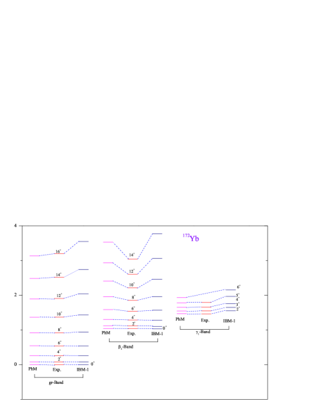
Figure 2:

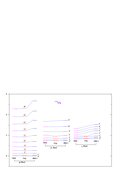
Figure 3:

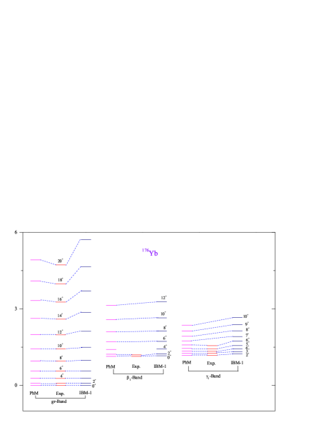
Figure 4:

References

- [1] J N Mo et al. Nucl. Phys. A472 295 (1987)
- [2] S Jonsson, N Roy, H Ryde, W Walus et al. Nucl. Phys. A 449 537 (1986)
- [3] E M Beck, J C.Bcelar, M A Deleplanque, R M Diamond et al. Nucl. Phys. A 464 472 (1987)
- [4] T Byrski et al. Nucl. Phys. A 474 193 (1987)
- [5] M P Fewell et al. Phys. Rev. C 37 101 (1988)
- [6] C Granja, S Posíšil, R E Chrien and S.A.Telezhnikovc Nucl. Phys. A 757 287 (2005)
- [7] I Y Lee et al. Phys. Rev. C 56 753 (1997)
- [8] K Hara and S Iwasaki Nucl. Phys. A 348 200 (1980)
- [9] K Hara and S Iwasaki Nucl. Phys. A 430 175 (1984)
- [10] K Hara and Y Sun Nucl. Phys. A 529 445 (1991)
- [11] K Hara and Y Sun Nucl. Phys. A 531 221 (1991)
- [12] K Hara and Y Sun Nucl. Phys. A 537 77 (1992)
- [13] Y Sun and J L Egido Nucl. Phys. A 580 1 (1994)
- [14] D E Archer et al. Phys. Rev. C 57 2924 (1998)
- [15] W Gelletly et al. J. Phys. G: Nucle. Phys. 13, 69 (1987)
- [16] Ph N Usmanov and I N Mikhailov Phys. Part. Nucl. Lett. 28, 348 (1997) [Fiz.Elem.Chastits At. Yadra 28, 887 (1997)]
- [17] Ph N Usmanov, A A Okhunov, U S Salikhbaev and A Vdovin Phys. Part. Nucl. Lett. 7, 185 (2010) [Fiz.Elem.Chastits At. Yadra 159, 306 (2010)]
- [18] S M Harris Phys. Rev. B 138 509, (1965)
- [19] A Arima and F Iachello Ann. Phys. NY 99 253 (1976)
- [20] A Arima and F Iachello Ann. Phys. NY 111 201 (1978)
- [21] A Arima and F Iachello Ann. Phys. NY 123 468 (1979)
- [22] O Scholten, F Iachello, and A Arima Ann. Phys. NY 115 325 (1978)
- [23] R F Casten and D D Warner Rev. Mod. Phys. 60 389 (1988)
- [24] R Bengtsson and S Fraundorf Nucl.Phys. A 327 139 (1979)
- [25] R B Begzhanov et al. Handbook on Nuclear Physics Vol 1.2 (Tashkent: FAN) (1989)
- [26] C M Baglin Nucl. Data. Sheets 96 611 (2002)
- [27] B Singh Nucl. Data. Sheets 75 199 (1995)
- [28] E Browne and H Junde Nucl. Data. Sheets 87 15 (1999)
- [29] M S Basunia Nucl. Data. Sheets 107 791 (2006)
- [30] http://www.nndc.bnl.gov/chart/getENSDFDatasets.jsp