Galaxies with Supermassive Binary Black Holes:
(II) A Model with Cuspy Galactic Density Profiles

Abstract

The existence and uniqueness of equilibrium points, including Lagrange Points and Jiang-Yeh Points, of a galactic system with supermassive binary black holes embedded in a centrally cuspy galactic halo are investigated herein. Differing from the previous results of non-cuspy galactic profiles that Jiang-Yeh Points only exist under a particular condition, it is found here that the Lagrange Points, L2, L3, L4 and L5, Jiang-Yeh Points, JY1 and JY2, exist under general conditions. The stability analysis shows that L2, L3, JY1 and JY2 are unstable. However, L4 and L5 are only unstable when the galactic total mass is smaller than a critical mass; otherwise they become neutrally stable centers. These results will be important for further studies on the cores of early-type galaxies.

1 Introduction

The general structure of galaxies has been one of the most interesting astronomical subjects due to the beauty and diversity of their morphological shapes. It is also an important research field in that galaxies are building blocks of the universe; so the formation and evolution of galactic structures, which are imprints left by the interactions of galaxies, can trace the history of the universe.

Through astronomical observations, the interaction between galaxies is confirmed to be taking place frequently, for example, the mergers of mice galaxies (NGC 4674 A&B), NGC 2207/IC 2163 and NGC 2623. These results have triggered many further investigations related to mergers. For example, Wu & Jiang (2009) showed that the inter-galactic population could be ejected from galaxies during merging events. Furthermore, the ring galaxies are likely to be the outcome of major mergers, as shown in Wu & Jiang (2012).

On the other hand, it is generally believed that there is a supermassive black hole at the center of galaxies. A merger of two galaxies with supermassive black holes is likely to form a supermassive binary black hole (SBBH) near the center of the newly formed galactic merging system. In fact, the major mergers of two disk galaxies are believed to be the main mechanism forming elliptical galaxies. This is partially due to the fact that elliptical galaxies are generally massive and gas-poor, and major mergers can produce a larger galactic system and reduce the gaseous component by rapid star formation or gas diffusion during merging processes. Thus, the investigations on the dynamics of elliptical galaxies are usually based on the gas-poor assumption.

In order to study the dynamic evolution of SBBH, Quinlan (1996) carried out numerical experiments on the scattering processes for the restricted three-body problem. The main issue addressed in that work was the SBBH hardening. In fact, modifications of the restricted three body problem were employed to model various problems related to planetary systems (Chermnykh 1987; Papadakis 2004, 2005a, 2005b, Jiang & Yeh 2006; Yeh & Jiang 2006; Kushvah 2008a, 2008b, 2009, 2011a, 2011b, 2012). In addition, the discoveries of extra-solar planets have triggered many investigations in the field of planetary systems (see Jiang & Ip 2001; Ji et al. 2002; Jiang & Yeh 2003, 2004a, 2004b, 2004c, 2007, 2009, 2011; Jiang et al. 2003, 2006, 2007, 2009, 2010, 2013; Chatterjee et al. 2008).

Milosavljevic and Merritt (2001) used N-body simulations to investigate the orbital decay of black holes and the formation of SBBHs during galactic mergers. They found that it only takes about a million years for black holes to sink to the center and become a hard binary. However, they claimed that black holes stall at separations of sub-parsec scales. Then, Yu (2002) semi-analytically estimated the possible time-scales to form SBBHs and found that the time-scale of dynamical friction is too long for small black holes to sink into the center, so it is difficult to form SBBHs with very small mass ratio. Thus, the SBBHs with moderate mass ratios are most likely to form and survive with semi-major axes around $10^{-3}$ to $10$ pc in spherical or nearly spherical galaxies.

Moreover, in order to explain the surface brightness of NGC 3706, Kandrup et al. (2003) considered the stellar dynamics under the gravitational fields of SBBH and a fixed galactic potential. They found that the transition between the inner and outer power-law profiles predicted by a Dehnen potential is too gradual to represent real galaxies, so the Nuker law was used in their model.

Motivated by the above work, as in Kandrup et al. (2003), a model of modified restricted three body problems was used in Jiang & Yeh (2014) to study a galactic system with SBBH. Both Kandrup et al. (2003) and Jiang & Yeh (2014) employed the Nuker law as their three dimensional spherical galactic density profiles because the Nuker law is a simple and neat way to present a smooth broken power-law with two power-indexes, and the transition is located at a well defined radius, i.e. the break radius. Note that the Nuker law was originally introduced in Lauer et al. (1992) to fit the two dimensional surface brightness of M32, and later for other galaxies in Lauer et al. (1995). In order to make it clear, we will use the term spherical Nuker law to name the galactic density profiles in this paper.

Jiang & Yeh (2014) discovered that when the galactic density profile is a spherical Nuker law with $\gamma=0$ (i.e. no cusp), $\alpha=2$, $\beta=4$, the usual five Lagrange Points always exist, and the new equilibrium points, i.e. Jiang-Yeh Points, exist if and only if the total galactic mass is larger than the critical mass. The analytic expression of this critical mass was provided and the stability analysis was performed. These results give important implications for the orbital evolution near the centers of galaxies with SBBH, and lead to a possible mechanism to form the cores of early-type galaxies through the existence of unstable Jiang-Yeh Points near supermassive black holes.

However, because the cuspy density profile is expected for the dark matter halo through cosmological simulations, it will be interesting to investigate the existence of Jiang-Yeh Points in a system with SBBH and a central cusp. For spherical Nuker law, i.e. Eq.(6) of Jiang & Yeh (2014), the density profile has a cuspy center when $\gamma\geq 1$. We find that when $\alpha=2$, $\beta=5$, $\gamma=1$, the corresponding gravitational potential of the density profile has an analytic form. Therefore, in this paper, we study the dynamics of a system wherein a test particle moves under the influence of SBBH and a galactic potential, which is dominated by a cuspy dark matter halo following a spherical Nuker law with $\alpha=2$, $\beta=5$, $\gamma=1$. We will investigate the existence of equilibrium points and also perform the stability analysis of these points.

We present our model in Section 2, and the analytical results for the existence of equilibrium points are in Section 3. The bifurcation diagrams, locations of equilibrium points and zero-velocity curves are shown in Section 4. The stability analysis is presented in Section 5, and the concluding remarks are offered in Section 6.

2 The Model

We consider the motion of test particles influenced by the gravitational force from the central binary black holes and the galaxy. The test particles are considered to move on the same plane of the orbital plane of binary black holes.

For the description below, those parts which are exactly the same as the equations in Jiang & Yeh (2014) will be skipped (refer to Jiang & Yeh 2014). After the procedure of non-dimensionalization as done in Yeh et al. (2012) and Jiang & Yeh (2014), in which the scale length is set to be the break radius, i.e. $L_{0}=r_{b}$, the density profile of the galaxy is expressed as:

$$\rho=\rho_{c}r^{-1}\left\{1+r^{2}\right\}^{-2}\,.$$ (1)

where $\rho_{c}$ is a constant; $r$ is the distance (in the unit of break radius $r_{b}$) from the origin in this spherical distribution. This profile gives an NFW central cusp (Navarro, Frenk, White 1995) and also a realistic sharper outer edge, i.e. when $r\to 0$, the density $\rho\propto r^{-1}$ is the cusp in NFW profile; when $r>>1$, the density decays as $\rho\propto r^{-5}$ which is sharper than the NFW’s profile ($\rho\propto r^{-3}$ for $r>>1$). Because NFW profile is not for an equilibrium galaxy (Binney & Trmaine 2008), our profile is a more realistic model for the system considered here. Note that all variables, functions and parameters, such as mass, potential, radius, normalization constants etc., are all written as dimensionless quantities in this paper.

The mass of the galaxy up to $r$ is thus:

$$M(r)=2\pi\rho_{c}\left\{1-\frac{1}{1+r^{2}}\right\}.$$ (2)

If the total galactic mass is $M_{g}$, we have $\rho_{c}=\frac{M_{g}}{2\pi}$. The corresponding potential is:

$$V(r)=-4\pi\left[\frac{1}{r}\int_{0}^{r}\rho(r^{\prime}){r^{\prime}}^{2}dr^{\prime}+\int_{r}^{\infty}\rho(r^{\prime})r^{\prime}dr^{\prime}\right]=-M_{g}\left\{\frac{\pi}{2}-\tan^{-1}r\right\},$$ (3)

Moreover, from the potential, we can obtain the gravitational force as:

$$f_{g}(r)\equiv-\frac{\partial V}{\partial r}=-M_{g}\left(\frac{1}{1+r^{2}}\right).$$ (4)

Considering the motion on the $x-y$ plane of the rotating frame, binary black holes, each with mass $m$ at $(R,0)$, $(-R,0)$, and a test particle located on $x,y$ with velocity $u$, $v$, the equations of motion would be as follows:

$$\left\{\begin{array}[]{ll}&\frac{dx}{dt}=u\\ &\frac{dy}{dt}=v\\ &\frac{du}{dt}=2nv+n^{2}x-\frac{m(x+R)}{r_{1}^{3}}-\frac{m(x-R)}{r_{2}^{3}}-\frac{M_{g}x}{r}\left(\frac{1}{1+r^{2}}\right),\\ &\frac{dv}{dt}=-2nu+n^{2}y-\frac{my}{r_{1}^{3}}-\frac{my}{r_{2}^{3}}-\frac{M_{g}y}{r}\left(\frac{1}{1+r^{2}}\right),\end{array}\right.$$ (5)

where $r_{1}=\sqrt{(x+R)^{2}+y^{2}}$, $r_{2}=\sqrt{(x-R)^{2}+y^{2}}$, $r=\sqrt{x^{2}+y^{2}}$ and $n$ is the angular velocity of black holes. That is, in the inertial frame, each black hole moves along the circular orbit at $r=R$ with an angular velocity, i.e. mean motion:

$$n=\left\{\frac{m}{4R^{3}}+\frac{1}{R}|f_{g}(R)|\right\}^{1/2}=\left\{\frac{m}{4R^{3}}+\frac{M_{g}}{R(1+R^{2})}\right\}^{1/2}$$ (6)

The corresponding Jacobi integral of this system is similar as the one in Jiang & Yeh (2006, 2014):

$$C_{J}=-u^{2}-v^{2}+n^{2}(x^{2}+y^{2})+\frac{2m}{r_{1}}+\frac{2m}{r_{2}}+2M_{g}\left\{\frac{\pi}{2}-\tan^{-1}(\sqrt{x^{2}+y^{2}})\right\}.$$ (7)

3 The Equilibrium Points

The existence and uniqueness of equilibrium points are investigated in this section. We follow the convention introduced in Jiang & Yeh (2014) in naming the equilibrium points except that due to the singular property of the central point of the system, the origin will be named as the singular point. Because the singular point is not considered as an equilibrium point in our system, there will be no stability analysis of this point. The existence and uniqueness of Lagrange Points L4 and L5 will be presented in Theorem 1. The existence and uniqueness of Lagrange Points L2 and L3, and the singularity of the origin of the system will be presented in Theorem 2. The existence and uniqueness of Jiang-Yeh Points JY1 and JY2, will be presented in Theorem 3.

In general, for System (5), equilibrium points $(x_{e},y_{e})$ satisfy $A(x_{e},y_{e})=0$ and $B(x_{e},y_{e})=0$, where:

$$A(x,y)=n^{2}x-\frac{m(x+R)}{r_{1}^{3}}-\frac{m(x-R)}{r_{2}^{3}}-\frac{M_{g}x}{r}\frac{1}{(1+r^{2})},$$ (8)

$$B(x,y)=n^{2}y-\frac{my}{r_{1}^{3}}-\frac{my}{r_{2}^{3}}-\frac{M_{g}y}{r}\frac{1}{(1+r^{2})}.$$ (9)

For convenience, for $y\neq 0$, we define:

$$h(y)\equiv\frac{B(0,y)}{y}=n^{2}-\frac{2m}{\left[R^{2}+y^{2}\right]^{3/2}}-\frac{M_{g}}{|y|}\frac{1}{(1+y^{2})}$$ (10)

and

$$k(x)\equiv A(x,0)=n^{2}x-\frac{m(x+R)}{|x+R|^{3}}-\frac{m(x-R)}{|x-R|^{3}}-\frac{M_{g}x}{|x|}\frac{1}{(1+x^{2})}$$ (11)

From the results in Jiang & Yeh (2006), we have the following remarks:
Remark A:
For $y_{e}\neq 0$, $y_{e}$ satisfies $h(y)=0$, if and only if $(0,y_{e})$ is the equilibrium point of System (5).
Remark B:
$x_{e}$ satisfies $k(x)=0$, if and only if $(x_{e},0)$ is the equilibrium point of System (5).
Then, Remark (A) will be used to study the equilibrium points L4 and L5 in Theorem 1. Remark (B) will be used for all other points in Theorem 2 and 3.

Theorem 1: The Existence and Uniqueness of Lagrange Points L4 and L5
There is one and only one $\bar{y_{1}}>0$ such that $h(\bar{y_{1}})=0$, and only one $\bar{y_{2}}<0$ such that $h(\bar{y_{2}})=0$. That is, excluding the origin (0,0) of $x-y$ plane, there are two equilibrium points on the $y$-axis, i.e. L4 and L5, for System (5).

Proof:

We define

$$P(y)\equiv\frac{2m}{\left[R^{2}+y^{2}\right]^{3/2}}-n^{2}$$ (12)

$${\rm and}\qquad Q(y)\equiv\frac{-M_{g}}{|y|(1+y^{2})}$$ (13)

so from Eq.(10), we have $h(y)=-P(y)+Q(y)$.

At first, we consider the case when $y>0$. Because $\lim_{y\to 0}Q(y)=-\infty$, we have:

$$\lim_{y\to 0}h(y)=\lim_{y\to 0}-P(y)+Q(y)=-\infty;$$ (14)

and since $\lim_{y\to\infty}P(y)=-n^{2}$, $\lim_{y\to\infty}Q(y)=0$, we have $\lim_{y\to\infty}h(y)=n^{2}>0$. Moreover, from Eqs.(12)-(13), we have:

$$P^{\prime}(y)=-6my\left[R^{2}+y^{2}\right]^{-5/2},$$ (15)

and

$$Q^{\prime}(y)=M_{g}\frac{1+3y^{2}}{y^{2}(1+y^{2})^{2}}.$$ (16)

Since $P^{\prime}(y)<0$ and $Q^{\prime}(y)>0$, $h^{\prime}(y)=-P^{\prime}(y)+Q^{\prime}(y)>0$ for any $y>0$. Thus, $h(y)$ is a monotonically increasing function for any $y\in(0,\infty)$. With $\lim_{y\to 0}h(y)=-\infty$ and $\lim_{y\to\infty}h(y)>0$, we conclude there is a unique point $\bar{y_{1}}>0$ such that $h(\bar{y_{1}})=0$.

For the case when $y<0$, from Eqs.(15)-(16), we have $P^{\prime}(y)>0$,$Q^{\prime}(y)<0$, so $h(y)$ is a monotonically decreasing function. We also have $\lim_{y\to\-\infty}h(y)=n^{2}>0$ and $\lim_{y\to 0}h(y)=-\infty$. Thus, we find that there is a unique point $\bar{y_{2}}<0$ such that $h(\bar{y_{2}})=0$. $\Box$

Now we investigate the existence of equilibrium points on the $x$-axis. For convenience, we define

$$S(x)\equiv\frac{m(x+R)}{|x+R|^{3}}+\frac{m(x-R)}{|x-R|^{3}}-n^{2}x,$$ (17)

and therefore,

$$S(x)=\left\{\begin{array}[]{lll}&\frac{m}{(x+R)^{2}}+\frac{m}{(x-R)^{2}}-n^{2}x,&\quad{\rm for}\,\,x>R,\\ &\frac{m}{(x+R)^{2}}-\frac{m}{(x-R)^{2}}-n^{2}x,&\quad{\rm for}\,\,-R<x<R,\\ &-\frac{m}{(x+R)^{2}}-\frac{m}{(x-R)^{2}}-n^{2}x,&\quad{\rm for}\,\,x<-R.\end{array}\right.$$ (18)

We also define:

$$T(x)\equiv-\frac{M_{g}x}{|x|(1+x^{2})}.$$ (19)

From Eqs.(11), (17) and (19), we have:

$$k(x)=-S(x)+T(x).$$ (20)

In the following Theorem 2, the results show that Lagrange Points L2 and L3 exist. However, due to the singular property, the origin (0,0) is a singular point, though the net force shall be physically balanced there. In Theorem 3, it is shown that another two equilibrium points, JY1 and JY2, exist. JY1 is in the region $(-R,0)$ and JY2 is in the region $(0,R)$ of x-axis.

Theorem 2: The Existence and Uniqueness of Lagrange Points L2 and L3 and the Singularity of the Origin Point (0,0)
(i) There is an unique $x_{1}>R$ such that $k(x_{1})=0$ and an unique $x_{2}<-R$ such that $k(x_{2})=0$. That is, on the $x$-axis, there is one and only one equilibrium point in the region $(R,\infty)$, i.e. L2, and there is one and only one equilibrium point in the region $(-\infty,-R)$, i.e. L3.
(ii) Due to the singularity at $x=0$, the origin is not an equilibrium point (i.e. $k(0)\neq 0$), but is a singular point.

Proof of (i):

When $x>R$, from Eqs. (18)-(20),

$$k(x)=-S(x)+T(x)=-\frac{m}{(x+R)^{2}}-\frac{m}{(x-R)^{2}}+n^{2}x-\frac{M_{g}}{1+x^{2}}$$

$${\rm and}\quad k^{\prime}(x)=-S^{\prime}(x)+T^{\prime}(x)=\frac{2m}{(x+R)^{3}}+\frac{2m}{(x-R)^{3}}+n^{2}+\frac{2xM_{g}}{(1+x^{2})^{2}}>0.$$

Thus, we have $\lim_{x\to R^{+}}k(x)=-\infty$, $\lim_{x\to\infty}k(x)=\infty$. Moreover, from $k^{\prime}(x)>0$, we know that $k(x)$ is a monotonic function. Therefore, there is a unique $x_{1}>R$, such that $k(x_{1})=0$.

When $x<-R$, similarly, since $k^{\prime}(x)>0$, $\lim_{x\to-R^{-}}k(x)=\infty$, and $\lim_{x\to-\infty}k(x)=-\infty$, there is a unique $x_{2}<-R$ such that $k(x_{2})=0$. $\Box$

Proof of (ii):

When $-R<x<R$, from Eq. (18), we have:

$$S(x)=\frac{m}{(x+R)^{2}}-\frac{m}{(x-R)^{2}}-n^{2}x,$$ (21)

Thus, $S(0)=0$. Moreover, from Eq.(19), we have :

$$\lim_{x\to 0^{+}}T(x)=\lim_{x\to 0^{+}}-\frac{M_{g}}{(1+x^{2})}=-M_{g}$$

and

$$\lim_{x\to 0^{-}}T(x)=\lim_{x\to 0^{-}}-\frac{M_{g}x}{(-x)(1+x^{2})}=M_{g},$$

so $\lim_{x\to 0}T(x)$ does not exist. Therefore, $k(x)$ is not a continuous function at $x=0$, and so the origin (0,0) is a singular point. $\Box$

Theorem 3: The Existence and Uniqueness of Jiang-Yeh Points JY1 and JY2
There is a unique $x_{3}\in(0,R)$ such that $k(x_{3})=0$ and a unique $x_{4}\in(-R,0)$ such that $k(x_{4})=0$. That is, on the $x$-axis, there is one and only one equilibrium point in the region $(0,R)$, i.e. JY1, and there is one and only one equilibrium point in the region $(-R,0)$, i.e. JY2.

Proof:

When $-R<x<R$, from Eq.(21), we have:

$$S^{\prime}(x)=-\frac{2m}{(x+R)^{3}}+\frac{2m}{(x-R)^{3}}-n^{2}<0.$$ (22)

We first consider the region with $0<x<R$. From Eq.(19):

$$T^{\prime}(x)=-\frac{-2xM_{g}}{(1+x^{2})^{2}}=\frac{2xM_{g}}{(1+x^{2})^{2}}>0,$$ (23)

we have $k^{\prime}(x)=-S^{\prime}(x)+T^{\prime}(x)>0$, and thus $k(x)$ is a monotonic function in this region. Due to the singularity at 0 for $T(x)$ and at $R$ for S(x), we consider the limits and find $\lim_{x\to 0^{+}}k(x)=-S(0)+\lim_{x\to 0^{+}}T(x)=-M_{g}$ and $\lim_{x\to R^{-}}k(x)=-\lim_{x\to R^{-}}S(x)+T(R)=\infty$. Thus, there is a unique $x_{3}\in(0,R)$ such that $k(x_{3})=0$.

Similarly, for the region with $-R<x<0$, from Eq.(19):

$$T^{\prime}(x)=\frac{-2xM_{g}}{(1+x^{2})^{2}}>0,$$ (24)

so we have $k^{\prime}(x)=-S^{\prime}(x)+T^{\prime}(x)>0$ and $k(x)$ is a monotonic function in this region. Because $\lim_{x\to-R^{+}}k(x)=-\infty$ and $\lim_{x\to 0^{-}}k(x)=M_{g}>0$, there is a unique $x_{4}\in(-R,0)$ such that $k(x_{4})=0$.$\Box$

4 The Bifurcations and Zero-Velocity Curves

In order to demonstrate the analytic results proved above, we numerically determine the locations of equilibrium points by solving $k(x)=0$. The locations of the equilibrium points on the x-axis with $m=1$ as a function of $M_{g}$ are shown in Figs.1-2. Fig. 1(a) is for $R=0.25$, Fig. 1(b) is for $R=0.5$, Fig. 2(a) is for $R=1$ and Fig. 2(b) is for $R=2$.

It is clear that when $M_{g}=0$, there are three equilibrium points, L1, L2 and L3 on $x-$axis; when $M_{g}>0$, there are four equilibrium points, L2, L3, JY1 and JY2 on $x-$axis. The separations between these equilibrium points are larger for larger $R$. Moreover, it is interesting that when $M_{g}$ increases from 0 to 20, the separation between L2 and L3 decreases, but the separation between JY1 and JY2 increases.

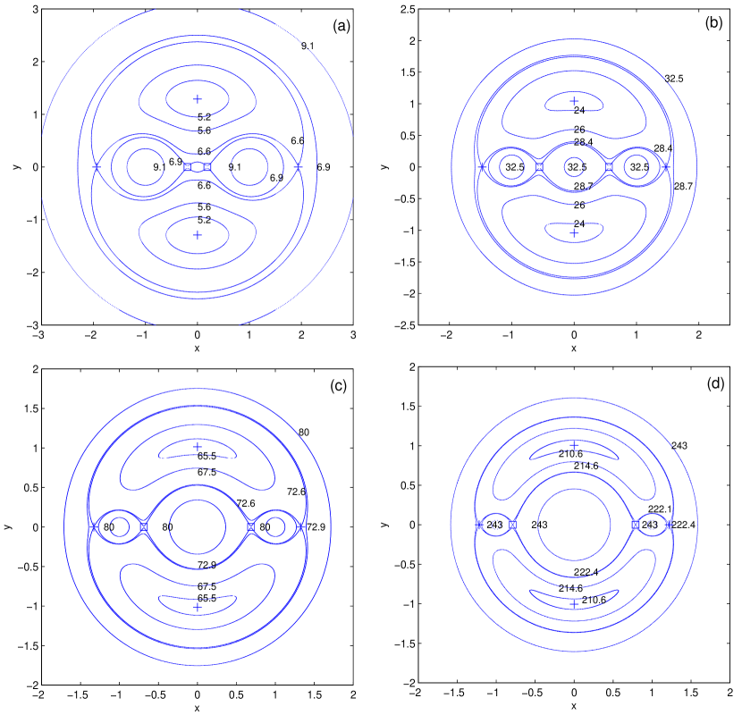
Figure 3: The zero-velocity curves of the system when $R=1$ and $m=1$, on which the corresponding values of the Jacobi integral $C_{J}$ are labeled. (a) is for $M_{g}=1$, (b) is for $M_{g}=10$, (c) is for $M_{g}=30$, (d) is for $M_{g}=100$. The $+$ signs indicate the locations of Lagrange Points and the squares indicate the locations of Jiang-Yeh Points.

In Fig. 3, the zero-velocity curves, which are obtained through Eq.(7), of the case with $m=1$ and $R=1$ are presented. Fig. 3(a) is for $M_{g}=1$, Fig. 3(b) is for $M_{g}=10$, Fig. 3(c) is for $M_{g}=30$ and Fig. 3(d) is for $M_{g}=100$. The $+$ signs are the locations for Lagrange Points, and the squares indicate the Jiang-Yeh Points. These points are numerically determined by solving $k(x)=0$ and $h(y)=0$. It is shown that they are completely consistent with the locations of equilibrium points implied by zero-velocity curves. The locations and the values of Jacobi integral $C_{J}$ of all equilibrium points shown in Fig. 3 are summarized in Table 1.

Table 1. The Locations and $C_{J}$ of Equilibrium Points

$M_{g}=1$		L2	L3	L4	L5	JY1	JY2
	$(x_{e},y_{e})$	(1.94,0)	(-1.94,0)	(0,1.29)	(0,-1.29)	(0.19,0)	(-0.19,0)
	$C_{J}$	6.58		5.02		6.94
$M_{g}=10$		L2	L3	L4	L5	JY1	JY2
	$(x_{e},y_{e})$	(1.47,0)	(-1.47,0)	(0,1.04)	(0,-1.04)	(0.56,0)	(-0.56,0)
	$C_{J}$	28.36		23.77		28.67
$M_{g}=30$		L2	L3	L4	L5	JY1	JY2
	$(x_{e},y_{e})$	(1.33,0)	(-1.33,0)	(0,1.01)	(0,-1.01)	(0.69,0)	(-0.69,0)
	$C_{J}$	72.58		65.20		72.90
$M_{g}=100$		L2	L3	L4	L5	JY1	JY2
	$(x_{e},y_{e})$	(1.22,0)	(-1.22,0)	(0,1.0)	(0,-1.0)	(0.79,0)	(-0.79,0)
	$C_{J}$	222.11		210.16		222.43

5 The Stability of Equilibrium Points

After the existence of equilibrium points is confirmed, and the locations of equilibrium points are determined, it would be interesting to understand the stability around these points. We now consider the following system:

$$\left\{\begin{array}[]{ll}&\frac{dx}{dt}=u,\\ &\frac{dy}{dt}=v,\\ &\frac{du}{dt}=2nv+A(x,y),\\ &\frac{dv}{dt}=-2nu+B(x,y),\end{array}\right.$$ (25)

where $A(x,y)$, $B(x,y)$ are defined in Eqs.(8)-(9).

To study the stability of equilibrium points, we need to know the properties of the eigenvalues of equilibrium points. The characteristic equation of the eigenvalue $\lambda$ is

$$\lambda^{4}+(4n^{2}-A_{x}-B_{y})\lambda^{2}+2n(A_{y}-B_{x})\lambda+A_{x}B_{y}-B_{x}A_{y}=0,$$ (26)

where $A_{x}\equiv{\partial A(x,y)}/{\partial x}$, $A_{y}\equiv{\partial A(x,y)}/{\partial y}$, $B_{x}\equiv{\partial B(x,y)}/{\partial x}$, and $B_{y}\equiv{\partial B(x,y)}/{\partial y}$. Thus,

$$A_{x}=n^{2}-\frac{m}{r_{1}^{3}}-\frac{m}{r_{2}^{3}}+\frac{3m(x+R)^{2}}{r_{1}^{5}}+\frac{3m(x-R)^{2}}{r_{2}^{5}}-\frac{M_{g}}{r(1+r^{2})}+\frac{M_{g}x^{2}(1+3r^{2})}{r(r+r^{3})^{2}},$$ (27)

$$A_{y}=\frac{3m(x+R)y}{r_{1}^{5}}+\frac{3m(x-R)y}{r_{2}^{5}}+\frac{M_{g}xy(1+3r^{2})}{r(r+r^{3})^{2}},$$ (28)

$$B_{x}=\frac{3my(x+R)}{r_{1}^{5}}+\frac{3my(x-R)}{r_{2}^{5}}+\frac{M_{g}xy(1+3r^{2})}{r(r+r^{3})^{2}},$$ (29)

$$B_{y}=n^{2}-\frac{m}{r_{1}^{3}}-\frac{m}{r_{2}^{3}}+\frac{3my^{2}}{r_{1}^{5}}+\frac{3my^{2}}{r_{2}^{5}}-\frac{M_{g}}{r(1+r^{2})}+\frac{M_{g}y^{2}(1+3r^{2})}{r(r+r^{3})^{2}}.$$ (30)

From Eqs.(28) and (29), for any $x_{e}$ we have $A_{y}(x_{e},0)=B_{x}(x_{e},0)=0$, and for any $y_{e}$ we have $A_{y}(0,y_{e})=B_{x}(0,y_{e})=0$. In order to do further investigation, some parameters need to be specified: we set $m=1$ and $R=1$ for all the results in this section. Thus, from Eq.(6) we have:

$$n^{2}=\frac{1}{4}+\frac{M_{g}}{2}.$$

At first, we consider the equilibrium point L2 and JY1, $(x_{e},y_{e})$, which satisfies $k(x_{e})=0$ with $x_{e}>0$ and $y_{e}=0$. Due to $A_{y}(x_{e},0)=0$ and $B_{x}(x_{e},0)=0$, Eq.(26) becomes:

$$\lambda^{4}+(4n^{2}-A_{x}-B_{y})\lambda^{2}+A_{x}B_{y}=0.$$ (31)

For convenience, we define $\Omega=A_{x}B_{y}$ and $\Pi\equiv A_{x}+B_{y}-4n^{2}$. Therefore, we have roots :

$$\lambda^{2}_{+}=\frac{\Pi+\sqrt{\Pi^{2}-4\Omega}}{2}\quad{\rm and}\quad\lambda^{2}_{-}=\frac{\Pi-\sqrt{\Pi^{2}-4\Omega}}{2}.$$ (32)

Moreover, $A_{x}(x_{e},0)$ and $B_{y}(x_{e},0)$ can be expressed as:

$$A_{x}(x_{e},0)=n^{2}+\frac{2}{|x_{e}+1|^{3}}+\frac{2}{|x_{e}-1|^{3}}+\frac{2x_{e}M_{g}}{(1+x_{e}^{2})^{2}}>0,$$ (33)

$$B_{y}(x_{e},0)=\frac{1}{x_{e}}\left(\frac{1}{|{x_{e}}+1|^{3}}-\frac{1}{|{x_{e}}-1|^{3}}\right)<0$$ (34)

(see Appendix A for details).

For L2, $x_{e}>R=1$, from Eqs. (33)-(34), since $A_{x}(x_{e},0)>0$ and $B_{y}(x_{e},0)<0$, we have $\Omega=A_{x}(x_{e},0)B_{y}(x_{e},0)<0$. Thus, $\Pi^{2}-4\Omega>0$, and we have $\lambda^{2}_{+}>0$ and $\lambda^{2}_{-}<0$. As in Szebehely (1967); this indicates that it is an unstable equilibrium point.

For JY1, it has $0<x_{e}<1$ and $y_{e}=0$. From Eqs. (33)-(34), $A_{x}(x_{e},0)>0$ and $B_{y}(x_{e},0)<0$, so $\Omega=A_{x}B_{y}<0$. Thus, $\Pi^{2}-4\Omega>0$, we have $\lambda^{2}_{+}>0$ and $\lambda^{2}_{-}<0$. Therefore, JY1 is also an unstable equilibrium point.

Because our system is symmetric with respect to the $y$-axis, the above results are also valid for L3 and JY2. Thus, the equilibrium points L3 and JY2 are unstable.

Secondly, we study the equilibrium point L4, which can be written as $(0,y_{e})$ with $y_{e}>0$. As mentioned previously, we have $A_{y}(0,y_{e})=B_{x}(0,y_{e})=0$. Thus, Eqs.(31) and (32) are also valid here. We find that:

$$A_{x}(0,y_{e})=\frac{6}{(1+y_{e}^{2})^{5/2}}>0,$$ (35)

but cannot determine the sign of $B_{y}(0,y_{e})$ analytically here. Thus, for each given $M_{g}$, the location of L4, $(0,y_{e})$, and then the corresponding value of $B_{y}(0,y_{e})$, $\Pi^{2}-4\Omega$, and $\Pi$ are determined numerically, as shown in Fig. 4(a)-(c). From Fig. 4(a), we know $B_{y}(0,y_{e})>0$ and so $\Omega=A_{x}B_{y}>0$. Fig. 4(b) shows the value of $\Pi^{2}-4\Omega$ as a function of $M_{g}$. It is clear that $\Pi^{2}-4\Omega$ is not a monotonic function of $M_{g}$. There is a critical value $M_{cr}\sim 4.213$, such that when $0<M_{g}<M_{cr}$, we have $\Pi^{2}-4\Omega<0$; when $M_{g}\geq M_{cr}$, we have $\Pi^{2}-4\Omega\geq 0$. For the case when $\Pi^{2}-4\Omega<0$, both $\lambda^{2}_{+}$ and $\lambda^{2}_{-}$ are complex numbers. This leads to both $\lambda_{+}$ and $\lambda_{-}$ having a root which contains a positive real part, so that L4 is unstable. For the case when $\Pi^{2}-4\Omega\geq 0$, we need to know the value of $\Pi$. As shown in Fig. 4(c), we find that $\Pi<0$ for the considered value of $M_{g}$. We thus have $\lambda^{2}_{+}<0$ and $\lambda^{2}_{-}<0$. This leads to both $\lambda_{+}$ and $\lambda_{-}$ being pure imaginary numbers, so that L4 is a center.

Because our system is symmetric with respect to the $x$-axis, the above results are also valid for L5. Thus, the equilibrium point L5 is either an unstable point or a center.

6 Concluding Remarks

We have studied the existence and uniqueness of equilibrium points, including Lagrange Points and Jiang-Yeh Points, of a galactic system with supermassive binary black holes embedded in a central cuspy galactic halo. Due to the cuspy density profile and focusing on the case with an equal mass binary black hole, we found that the central origin is a singular point. We also found that the Lagrange Points, L2, L3, L4 and L5, and Jiang-Yeh Points, JY1 and JY2, always exist, i.e. there are six equilibrium points in the considered system. This differs from the previous results of non-cuspy galactic profiles that Jiang-Yeh Points only exist under a particular condition (Jiang & Yeh 2014).

The stability analysis was performed for these equilibrium points. It is found that the equilibrium points L2, L3, JY1 and JY2 are unstable. The equilibrium point L4 (L5) is unstable when the galactic total mass $M_{g}<M_{cr}$, and is a neutrally stable center when $M_{g}\geq M_{cr}$. This critical mass $M_{cr}$, which is about 4.213, is therefore an important condition for the stability of L4 and L5. These new results will be employed to investigate the cores of early-type galaxies in the near future.

Appendix A

The details of the calculations of $A_{x}(x_{e},0)$ and $B_{y}(x_{e},0)$ in Section 5 are presented here. If $m=R=1$, then $r_{1}^{2}=(x+1)^{2}+y^{2}$ and $r_{2}^{2}=(x-1)^{2}+y^{2}$. From Eq. (27),

$$A_{x}(x_{e},0)=n^{2}-\frac{1}{|x_{e}+1|^{3}}-\frac{1}{|x_{e}-1|^{3}}+\frac{3(x_{e}+1)^{2}}{|x_{e}+1|^{5}}-\frac{3(x_{e}-1)^{2}}{|x_{e}-1|^{5}}$$

$$\qquad\qquad\qquad-\frac{M_{g}}{|x_{e}|(1+x_{e}^{2})}+\frac{M_{g}x_{e}^{2}(1+3x_{e}^{2})}{|x_{e}|^{3}(1+x_{e}^{2})^{2}}$$

$$=n^{2}+\frac{2}{|x_{e}+1|^{3}}+\frac{2}{|x_{e}-1|^{3}}-\frac{M_{g}(1+x_{e}^{2})}{|x_{e}|(1+x_{e}^{2})^{2}}+\frac{M_{g}(1+3x_{e}^{2})}{|x_{e}|(1+x_{e}^{2})^{2}}$$

$$=n^{2}+\frac{2}{|x_{e}+1|^{3}}+\frac{2}{|x_{e}-1|^{3}}+\frac{2|x_{e}|M_{g}}{(1+x_{e}^{2})^{2}}>0.$$

On the other hand, from Remark B, since $(x_{e},0)$ is an equilibrium point, $k(x_{e})=0$. By Eq.(11) and $m=R=1$, we have

$$-\frac{M_{g}}{|x_{e}|(1+x_{e}^{2})}=\frac{(x_{e}+1)}{x_{e}|x_{e}+1|^{3}}+\frac{(x_{e}-1)}{x_{e}|x_{e}-1|^{3}}-n^{2}.$$ (36)

From Eq. (30) and Eq. (36), we have:

$$B_{y}(x_{e},0)=n^{2}-\frac{1}{|x_{e}+1|^{3}}-\frac{1}{|x_{e}-1|^{3}}-\frac{M_{g}}{|x_{e}|(1+x_{e}^{2})}$$

$$=n^{2}-\frac{x_{e}}{x_{e}|x_{e}+1|^{3}}-\frac{x_{e}}{x_{e}|x_{e}-1|^{3}}+\frac{(x_{e}+1)}{x_{e}|x_{e}+1|^{3}}+\frac{(x_{e}-1)}{x_{e}|x_{e}-1|^{3}}-n^{2}$$

$$=\frac{1}{x_{e}}\left(\frac{1}{|{x_{e}}+1|^{3}}-\frac{1}{|{x_{e}}-1|^{3}}\right)<0.$$

Figure 1: The locations of the equilibrium points on the $x$-axis with $m=1$ as a function of $M_{g}$. (a) is for $R=0.25$ and (b) is for $R=0.5$.

Figure 2: The locations of the equilibrium points on the $x$-axis with $m=1$ as a function of $M_{g}$. (a) is for $R=1$ and (b) is for $R=2$.

Figure 4: (a) The value of $B_{y}(0,y_{e})$ as a function of $M_{g}$ for L4. (b) $\Pi^{2}-4\Omega$ as a function of $M_{g}$ for L4. (c) $\Pi$ as a function of $M_{g}$ for L4.

References

- (1) Binney J., Tremaine S., 2008, Galactic Dynamics, Second Edition (Princeton University Press)
- (2) Chatterjee, S., Ford, E. B., Matsumura, S., Rasio, F. A., 2008, ApJ, 686, 580
- (3) Chermnykh, S. V., 1987, Vest. Leningrad Univ. 2, 10
- (4) Ji, J., Li, G., Liu, L., 2002, ApJ, 572, 1041
- (5) Jiang, I.-G., Ip, W.-H., 2001, A&A, 367, 943
- (6) Jiang, I.-G., Ip, W.-H., Yeh, L.-C., 2003, ApJ, 582, 449
- (7) Jiang, I.-G., Yeh, L.-C., 2003, Int. J. Bifurcation and Chaos, 13, 617
- (8) Jiang, I.-G., Yeh, L.-C., 2004a, AJ, 128, 923
- (9) Jiang, I.-G., Yeh, L.-C., 2004b, Int. J. Bifurcation and Chaos, 14, 3153
- (10) Jiang, I.-G., Yeh, L.-C., 2004c, MNRAS, 355, L29
- (11) Jiang, I.-G., Yeh, L.-C., 2006, Astrophysics and Space Science, 305, 341
- (12) Jiang, I.-G., Yeh, L.-C., 2007, ApJ, 656, 534
- (13) Jiang, I.-G., Yeh, L.-C., 2009, AJ, 137, 4169
- (14) Jiang, I.-G., Yeh, L.-C., 2011, MNRAS, 415, 2859
- (15) Jiang, I.-G., Yeh, L.-C., Hung, W.-L., Yang, M.-S., 2006, MNRAS, 370, 1379
- (16) Jiang, I.-G., Yeh, L.-C., Chang, Y.-C., Hung, W.-L., 2007, AJ, 134, 2061
- (17) Jiang, I.-G., Yeh, L.-C., Chang, Y.-C., Hung, W.-L., 2009, AJ, 137, 329
- (18) Jiang, I.-G., Yeh, L.-C., Chang, Y.-C., Hung, W.-L., 2010, ApJS, 186, 48
- (19) Jiang, I.-G. et al., 2013, AJ, 145, 68
- (20) Jiang, I.-G., Yeh, L.-C., 2014, Astrophysics and Space Science, 349, 881
- (21) Kandrup, H. E., Sideris, I. V., Terzic, B. Bohn, C. L., 2003, ApJ, 597, 111
- (22) Kushvah, B. S., 2008a, Astrophysics and Space Science, 315, 231
- (23) Kushvah, B. S., 2008b, Astrophysics and Space Science, 318, 41
- (24) Kushvah, B. S., 2009, Astrophysics and Space Science, 323, 57
- (25) Kushvah, B. S., 2011a, Astrophysics and Space Science, 332, 99
- (26) Kushvah, B. S., 2011b, Astrophysics and Space Science, 333, 49
- (27) Kushvah, B. S., Kishor, R., Dolas, U., 2012, Astrophysics and Space Science, 337, 115
- (28) Lauer, T. R. et al., 1992, AJ, 104, 552
- (29) Lauer, T. R. et al., 1995, AJ, 110, 2622
- (30) Milosavljevic, M., Merritt, D., 2001, ApJ, 563, 34
- (31) Navarro, J. F., Frenk, C. S., White, S. D. M., 1995, MNRAS, 275, 720
- (32) Papadakis, K. E., 2004, A&A, 425, 1133
- (33) Papadakis, K. E., 2005a, Astrophysics and Space Science, 299, 67
- (34) Papadakis, K. E., 2005b, Astrophysics and Space Science, 299, 129
- (35) Quinlan, G. D., 1996, New Astronomy, 1, 35
- (36) Szebehely, V., 1967, Theory of Orbits: The Restricted Problem of Three Bodies (London: Academic Press, Inc.)
- (37) Wu, Y.-T., Jiang, I.-G., 2009, MNRAS, 399, 628
- (38) Wu, Y.-T., Jiang, I.-G., 2012, ApJ, 745, 105
- (39) Yeh, L.-C., Chen, Y.-C., Jiang, I.-G., 2012, Int. J. Bifurcation and Chaos, 22, 1230040
- (40) Yeh, L.-C., Jiang, I.-G., 2006, Astrophysics and Space Science, 306, 189
- (41) Yu, Q., 2002, MNRAS, 331, 935