Gas-liquid coexistence for the bosons square-well fluid and the $\mbox{}^{4}$He binodal anomaly

Abstract

The binodal of a boson square-well fluid is determined as a function of the particle mass through the newly devised quantum Gibbs ensemble Monte Carlo algorithm [R. Fantoni and S. Moroni, to be published]. In the infinite mass limit we recover the classical result. As the particle mass decreases the gas-liquid critical point moves at lower temperatures. We explicitely study the case of a quantum delocalization de Boer parameter close to the one of $\mbox{}^{4}$He. For comparison we also determine the gas-liquid coexistence curve of $\mbox{}^{4}$He for which we are able to observe the binodal anomaly below the $\lambda$-transition temperature.

Soon after Feynman rewriting of quantum mechanics and quantum statistical physics in terms of the path integral R. P. Feynman (1948); Feynman (1972) it was realized that the new mathematical object could be used as a powerful numerical instrument.

The statistical physics community soon realized that a path integral could be calculated using the Monte Carlo method D. M. Ceperley (1995).

Consider a fluid of $N$ bosons at a given absolute temperature $T=1/k_{B}\beta$ with $k_{B}$ Boltzmann constant. Let the system of particles have a Hamiltonian $\hat{H}=-\lambda\sum_{i=1}^{N}\bm{\nabla}_{i}^{2}+\sum_{i<j}\phi(|\mathbf{r}_{i}-\mathbf{r}_{j}|)$ symmetric under particle exchange, with $\lambda=\hbar^{2}/2m$, $m$ the mass of the particles, and $\phi(|\mathbf{r}_{i}-\mathbf{r}_{j}|)$ the pair-potential of interaction between particle $i$ at $\mathbf{r}_{i}$ and particle $j$ at $\mathbf{r}_{j}$. The many-particles system will have spatial configurations $\{R\}$, with $R\equiv(\mathbf{r}_{1},\ldots,\mathbf{r}_{N})$ the coordinates of the $N$ particles. The partition function of the fluid can be calculated D. M. Ceperley (1995) as a sum over the $N!$ possible particles permutations, ${\cal P}$, of a path integral over closed many-particles paths $X\equiv(R_{0},\ldots,R_{P})$ in the imaginary time interval $\tau\in[0,\beta=P\epsilon]$, discretized into $P$ intervals of equal length $\epsilon$, the time-step, with $R_{P}={\cal P}R_{0}$ the $\beta$-periodic boundary condition.

More recently a grand canonical ensemble algorithm has been devised by Massimo Boninsegni et al. M. Boninsegni, N. Prokof’ev, and B. Svistunov (2006); *Boninsegni2006b for the path integral Monte Carlo method. This paved the way to the development of a quantum Gibbs ensemble Monte Carlo algorithm (QGEMC) to study the gas-liquid coexistence of a generic boson fluid R. Fantoni and S. Moroni (2014). This algorithm is the quantum analogue of Athanassios Panagiotopoulos A. Z. Panagiotopoulos (1987); *Panagiotopoulos88; *Smit89a; *Smit89b; *Frenkel-Smit method which has now been successfully used for several decades to study first order phase transitions in classical fluids A. Z. Panagiotopoulos (1992); *Sciortino2009; *Fantoni2013. However, like simulations in the grand-canonical ensemble, the method does rely on a reasonable number of successful particle insertions to achieve compositional equilibrium. As a consequence, the Gibbs ensemble Monte Carlo method cannot be used to study equilibria involving very dense phases. Unlike previous extensions of Gibbs ensemble Monte Carlo to include quantum effects (some F. Schneider, D. Marx, and P. Nielaba (1995); *Nielaba1996 only consider fluids with internal quantum states; others Q. Wang and J. K. Johnson (1997); *Georgescu2013; *Kowalczyk2013 successfully exploit the path integral Monte Carlo isomorphism between quantum particles and classical ring polymers, but lack the structure of particle exchanges which underlies Bose or Fermi statistics), the QGEMC scheme is viable even for systems with strong quantum delocalization in the degenerate regime of temperature. Details of the QGEMC algorithm will be presented elsewhere R. Fantoni and S. Moroni (2014).

In this communication we will apply the QGEMC method to the fluid of square well bosons in three spatial dimensions as an extension of the work of Vega et al. L. Vega, E. de Miguel, L. F. Rull, G. Jackson, and I. A. McLure (1992); *Liu2005 on the classical fluid. The de Boer quantum delocalization parameter $\Lambda=\hbar/\sigma(m{\cal E})^{1/2}$, with ${\cal E}$ and $\sigma$ measures of the energy and length scale of the potential energy, can be used to estimate the quantum mechanical effects on the thermodynamic properties of nearly classical liquids R. A. Young (1980). We will consider square well fluids with two values of the particle mass $m$: $\Lambda=1/\sqrt{50}$, close but different from zero, and $\Lambda=1/\sqrt{5}$. In the first case we compare our result with the one of Vega and in the second case with the one of $\mbox{}^{4}$He which we consider in our second application. When studying the binodal of $\mbox{}^{4}$He in three spatial dimensions we are able to reproduce the binodal anomaly appearing below the $\lambda$-point where the liquid branch of the coexistence curve shows a re-entrant behavior.

In our implementation of the QGEMC R. Fantoni and S. Moroni (2014) algorithm we choose the primitive approximation to the path integral action discussed in Ref. D. M. Ceperley (1995). The simulation is performed in two boxes (representing the two coexisting phases) of varying volumes $V_{1}$ and $V_{2}=V-V_{1}$ and numbers of particles $N_{1}=V_{1}\rho_{1}$ and $N_{2}=V_{2}\rho_{2}=N-N_{1}$ with $V$ and $N=V\rho$ constants. The Gibbs equilibrium conditions of pressures and chemical potentials equality between the two boxes is enforced by allowing changes in the volumes of the two boxes (the volume move, $q=5$) and by allowing exchanges of particles between the two boxes (the open-insert move, $q=1$, plus the complementary close-remove move, $q=2$, plus the advance-recede move, $q=3$) while at the same time sampling the closed paths configuration space (the swap move, $q=4$, plus the displace move, $q=6$, plus the wiggle move, $q=7$). We thus have a menu of seven, $q=1,2,\ldots,7$, different Monte Carlo moves where a single random attempt of any one of them with probability $G_{q}=g_{q}/\sum_{q=1}^{7}g_{q}$ constitutes a Monte Carlo step.

We denote with ${\cal V}$ the maximum displacement of $\ln(V_{1}/V_{2})$ in the volume move, with ${\cal L}^{(p)}$ the maximum particle displacement in box $p=1,2$ in the displacement move, and with ${\cal M}_{q}<P$ the maximum number of time slices involved in the $q\neq 5,6$ move. In order to fulfill detailed balance we must choose ${\cal M}_{1}={\cal M}_{2}$.

Letting the system evolve at a given absolute temperature $T$ from a given initial state (for example we shall take $\rho_{1}=\rho_{2}=\rho$) we measure the densities of the two coexisting phases, $\rho_{1}<\rho$ and $\rho_{2}>\rho$, which soon approach the coexistence equilibrium values.

First we study a system of bosons in three dimensions interacting with a square well pair-potential

$$\phi(r) = \left\{\begin{array}[]{ll}+\infty&r<\sigma\\ -{\cal A}&\sigma\leq r<\sigma(1+\Delta)\\ 0&\sigma(1+\Delta)\leq r\end{array}\right.$$ (4)

which, for example, can be used as an effective potential for cold atoms C. J. Pethik and H. Smith (2002) with a scattering length $a=\sigma(1+\Delta)[1-\tan(\sigma\Delta\sqrt{{\cal A}/2\lambda})/\sigma(1+\Delta)\sqrt{{\cal A}/2\lambda}]$. We choose ${\cal A}>0$ as the unit of energies and $\sigma$ as the unit of lengths. We then introduce a reduced temperature $T^{*}=k_{B}T/{\cal A}$ and a reduced density $\rho^{*}=\rho\sigma^{3}$. When the mass of the boson is very big, i.e. $\lambda^{*}=\lambda/({\cal A}\sigma^{2})\ll 1$ we are in the classical limit. The classical fluid has been studied originally by Vega et al. L. Vega, E. de Miguel, L. F. Rull, G. Jackson, and I. A. McLure (1992) who found that the critical point of the gas-liquid coexistence moves at lower temperatures and higher densities as $\Delta$ gets smaller. The quantum mechanical effects on the thermodynamic properties of nearly classical liquids can be estimated by the de Boer quantum delocalization parameter $\Lambda=\sqrt{2\lambda^{*}}$.

During the subcritical temperature runs we register the densities of the gas, $\rho_{g}$, and of the liquid, $\rho_{l}(>\rho_{g})$, phase (box). When the densities of the two boxes are too close one another we may observe curves crossing which implies that the two boxes exchange identity. It is then necessary the computation of a density probability distribution function, created using the densities of both boxes. When we are at temperatures sufficiently below the critical point, this distribution appears to be bimodal, i.e. it has two peaks approximated by Gaussians. In some representative cases we checked that the peaks of the bimodal so calculated occur at the same densities as the peaks of the bimodal obtained from the single density distribution of the worm algorithm after a careful tuning of the chemical potential N. B. Wilding (1995).

We study the model with $\Delta=0.5$ near their classical limit $\lambda^{*}=1/100$ ($\Lambda\approx 0.14,a^{*}=a/\sigma\approx 1.44$) and at an intermediate case $\lambda^{*}=1/10$ ($\Lambda\approx 0.45,a^{*}\approx 0.58$). We choose $N=50$, $\rho^{*}=0.3$, ${\cal L}^{(p)}=V_{p}^{1/3}/10$, ${\cal V}=1/10$, we take all ${\cal M}_{q}$ equal, adjusted so as to have the acceptance ratios of the wiggle move close to $50$%, $g_{1}=g_{2}=g_{3}=g_{4}=g_{7}=1$, $g_{5}=0.0001$, and $g_{6}=0.1$. Moreover we choose the relative weight of the Z and G sectors of our extended worm algorithm, $C$ M. Boninsegni, N. Prokof’ev, and B. Svistunov (2006), so as to have the Z-sector acceptance ratios close to $50$%. We started from an initial configuration where we have an equal number of particles in boxes of equal volumes at a total density $\rho^{*}=0.3$.

All our runs were made of $10^{5}$ blocks of $10^{5}$ MC steps with properties measurements every $10^{2}$ steps . The time needed to reach the equilibrium coexistence increases with $P$ and in general with a lowering of the temperature.

If we choose $\lambda^{*}=1/100$ and $P=2$, ${\cal M}_{q}=1$ (in this case the advance-recede move cannot occur) we find that our algorithm gives results close to the ones of Vega L. Vega, E. de Miguel, L. F. Rull, G. Jackson, and I. A. McLure (1992) obtained with the classical statistical mechanics ($\lambda^{*}=0$) algorithm of Panagiotopoulos A. Z. Panagiotopoulos (1987); B. Smit, Ph. De Smedt, and D. Frenkel (1989); B. Smit and D. Frenkel (1989) . As we diminish the time-step $\epsilon^{*}=1/PT^{*}$ at a given temperature we can extrapolate to the zero time-step limit $P\to\infty$ as shown in Fig. 2. We thus obtain the fully quantum statistical mechanics result for the binodal shown in Fig. 1 which turns out to exist for $T^{*}\lesssim 1$. This shows that the critical point due to the effect of the quantum statistics moves at lower temperatures. For the studied temperatures the superfluid fraction E. L. Pollock and D. M. Ceperley (1987) of the system was always negligible as in the systems studied in Ref. Q. Wang and J. K. Johnson (1997); *Georgescu2013; *Kowalczyk2013 like Neon ($\Lambda\approx 0.095$) and molecular Hydrogen ($\Lambda\approx 0.276$).

In order to extrapolate the binodal to the critical point we used the law of “rectilinear diameters”, $\rho_{l}+\rho_{g}=2\rho_{c}+a|T-T_{c}|$, and the Fisher expansion M. E. Fisher (1966), $\rho_{l}-\rho_{g}=b|T-T_{c}|^{\beta_{1}}(|T-T_{c}|+c)^{\beta_{0}-\beta_{1}}$, with $\beta_{1}=1/2$ and $\beta_{0}=0.3265$, and $a,b,c$ fitting parameters with $c=0$ for $\lambda=0$ and $c\neq 0$ for $\lambda\neq 0$.

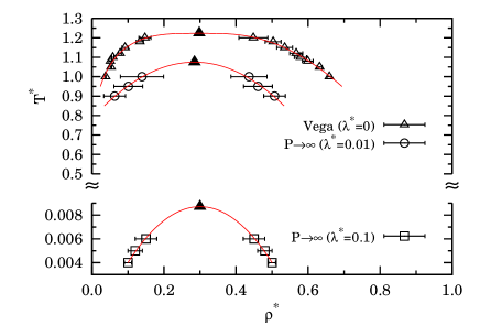
Figure 1: (color online) Binodal for the square well fluid in three dimensions. Shown are the classical results of Vega et al. L. Vega, E. de Miguel, L. F. Rull, G. Jackson, and I. A. McLure (1992) at $\lambda^{*}=0$ and our results in the $P\to\infty$ limit for $\lambda^{*}=1/100,1/10$. In the simulations we used $N=50$ and for the extrapolation to the zero time-step limit up to $P=20$ for $\lambda^{*}=1/100$ and $P=500$ for $\lambda^{*}=1/10$. The curves extrapolating to the critical point are obtained as described in the text. The filled triangles are the expected critical points.

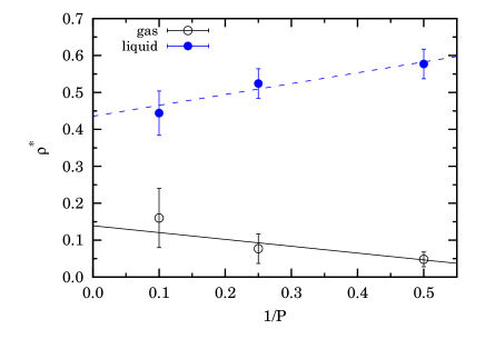
Figure 2: (color online) Linear fit to the zero time-step limit $P\to\infty$ for $T^{*}=1$ and $\lambda^{*}=1/100$.

Upon increasing $\lambda^{*}$ to $1/10$ the binodal now appears at $T^{*}\lesssim 0.008$ where we had a non negligible superfluid fraction E. L. Pollock and D. M. Ceperley (1987) ($\rho_{s}/\rho\approx 0.32(2)$ at $T^{*}=0.006$ on the liquid branch). As a consequence it proves necessary to use bigger $P$ in the extrapolation to the zero time-step limit. Notice also that at lower temperature it is necessary to run longer simulations due to the longer paths and equilibration times. We generally expect that increasing $\lambda^{*}$ the gas-liquid critical temperature decreases and the normal-super fluid critical temperature increases. So the window of temperature for the normal liquid tends to close.

Our second study is on $\mbox{}^{4}$He, for which $\lambda^{*}=6.0596$. We now take $1$Å as unit of lengths and $k_{B}$K as unit of energies. In this case $\sigma\approx 2.5$Å, ${\cal E}\approx 10.9$K, and $\Lambda\approx 0.42$. A situation comparable to the square well case with $\lambda^{*}=1/10$. We use $N=128$ and the Aziz HFDHE2 pair-potential R. A. Aziz, V. P. S. Nain, J. S. Carley, W. L. Taylor, and G. T. McConville (1979)

$$\phi(r) = \left\{\begin{array}[]{ll}\epsilon\phi^{*}(x)&r<r_{\text{cut}}\\ 0&r\geq r_{\text{cut}}\end{array}\right.,$$ (7)

$$\phi^{*}(x) = A\exp(-\alpha x)-\left(\frac{C_{6}}{x^{6}}+\frac{C_{8}}{x^{8}}+\frac{C_{10}}{x^{10}}\right)F(x),$$ (8)

$$F(x) = \left\{\begin{array}[]{ll}\exp[-(D/x-1)^{2}]&x<D\\ 1&x\geq D\end{array}\right.,$$ (11)

where $x=r/r_{m}$, $r_{m}=2.9673$, $\epsilon/k_{B}=10.8$, $A=0.5448504$, $\alpha=13.353384$, $C_{6}=1.3732412$, $C_{8}=0.4253785$, $C_{10}=0.178100$, $D=1.241314$, and $r_{\text{cut}}=6$Å (here we explicitly checked that during the simulation the conditions $V_{p}^{1/3}>2r_{\text{cut}}$ for $p=1,2$ are always satisfied). In this case it proves convenient to choose $\rho^{*}=0.01$, ${\cal L}^{(p)}=V_{p}^{1/3}/10$, ${\cal V}=1/10$, $g_{1}=g_{2}=g_{3}=g_{4}=g_{7}=1$, $g_{5}=0.0001$, and $g_{6}=0.1$. As for the SW case we observe a decrease of the width of the coexistence curve $\rho_{l}-\rho_{g}$ as the number of time slices increases. We thus work at a small (fixed) time-step $\epsilon^{*}=0.002$ about $1/1000$ of the superfluid transition temperature as advised in Ref. D. M. Ceperley (1995) to be necessary when studying Helium with the primitive approximation for the action.

The results for the binodal are shown in Fig. 3. The experimental critical point is at $T_{c}=5.25$K and $\rho_{c}=17.3$mol/l R. D. McCarty (1973); *McCarty1980. Factors explaining the discrepancy with experiment could be the size error or the choice of the pair-potential. Choosing bigger sizes $N$ it is possible to increase $r_{\text{cut}}$ and this shifts the simulated critical temperature to higher values. For the three dimensional $\mbox{}^{4}$He we expect to have the superfluid below a $\lambda$-temperature $T^{*}_{\lambda}=2.193(6)$ M. Boninsegni, N. V. Prokof’ev, and B. V. Svistunov (2006), so our results again show that our method works well even in the presence of a non negligible superfluid fraction. Moreover as shown by the points at the two lowest temperatures we are observing the expected H. Stein, C. Porthun, and G. Röpke (1998) binodal anomaly below the $\lambda$-point.

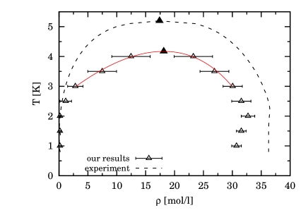
Figure 3: (color online) Binodal for the $\mbox{}^{4}$He of Aziz R. A. Aziz, V. P. S. Nain, J. S. Carley, W. L. Taylor, and G. T. McConville (1979) in three dimensions. In our simulations we used $N=128$, $r^{*}_{\text{cut}}=6$, and a time-step $\epsilon^{*}=0.002$. The continuous (red) curve extrapolating to the critical point are obtained as described in the text. The filled triangle is the estimated critical point. The experimental results from Ref. R. D. McCarty (1980) are also shown as a dashed curve.

In conclusion we determined the gas-liquid binodal of a square well fluid of bosons as a function of the particle mass and of $\mbox{}^{4}$He, in three spatial dimensions, from first principles. The critical point of the square well fluid moves to lower temperatures as the mass of the particles decreases, or as the de Boer parameter increases, while the critical density stays approximately constant.

Our results for $\mbox{}^{4}$He compare well with the experimental critical density even if a lower critical temperature is observed in the simulation. We expect this to be due mainly to a finite size effect unavoidable in the simulation. Nonetheless we are able to determine the binodal anomaly H. Stein, C. Porthun, and G. Röpke (1998) occurring below the $\lambda$-transition temperature. The anomaly that we observe in the simulation appears to be more accentuated than in the experiment and the liquid branch of the binodal falls at slightly lower densities.

Even if our QGEMC method is more efficient at high temperatures it is able to detect the liquid phase at low temperatures even below the superfluid transition temperature. The new numerical method is extremely simple to use and unlike current methods does not need the matching of free energies calculated separately for each phase or the simulation of large systems containing both phases and their interface.

R.F. would like to acknowledge the use of the PLX computational facility of CINECA through the ISCRA grant. We are grateful to Michael Ellis Fisher for correspondence and helpful comments.

References

- R. P. Feynman (1948) R. P. Feynman, Rev. Mod. Phys. 20, 367 (1948).
- Feynman (1972) R. P. Feynman, Statistical Mechanics: A Set of Lectures, Frontiers in Physics, Vol. 36 (W. A. Benjamin, Inc., 1972) notes taken by R. Kikuchi and H. A. Feiveson, edited by Jacob Shaham.
- D. M. Ceperley (1995) D. M. Ceperley, Rev. Mod. Phys. 67, 279 (1995).
- M. Boninsegni, N. Prokof’ev, and B. Svistunov (2006) M. Boninsegni, N. Prokof’ev, and B. Svistunov, Phys. Rev. Lett. 96, 070601 (2006).
- M. Boninsegni, N. V. Prokof’ev, and B. V. Svistunov (2006) M. Boninsegni, N. V. Prokof’ev, and B. V. Svistunov, Phys. Rev. E 74, 036701 (2006).
- R. Fantoni and S. Moroni (2014) R. Fantoni and S. Moroni, (2014), to be published.
- A. Z. Panagiotopoulos (1987) A. Z. Panagiotopoulos, Mol. Phys. 61, 813 (1987).
- A. Z. Panagiotopoulos, N. Quirke, M. Stapleton, and D. J. Tildesley (1988) A. Z. Panagiotopoulos, N. Quirke, M. Stapleton, and D. J. Tildesley, Mol. Phys. 63, 527 (1988).
- B. Smit, Ph. De Smedt, and D. Frenkel (1989) B. Smit, Ph. De Smedt, and D. Frenkel, Mol. Phys. 68, 931 (1989).
- B. Smit and D. Frenkel (1989) B. Smit and D. Frenkel, Mol. Phys. 68, 951 (1989).
- D. Frenkel and B. Smit (1996) D. Frenkel and B. Smit, Understanding Molecular Simulation (Academic Press, San Diego, 1996).
- A. Z. Panagiotopoulos (1992) A. Z. Panagiotopoulos, Mol. Sim. 9, 1 (1992).
- F. Sciortino, A. Giacometti, and G. Pastore (2009) F. Sciortino, A. Giacometti, and G. Pastore, Phys. Rev. Lett. 103, 237801 (2009).
- R. Fantoni and G. Pastore (2013) R. Fantoni and G. Pastore, Phys. Rev. E 87, 052303 (2013).
- F. Schneider, D. Marx, and P. Nielaba (1995) F. Schneider, D. Marx, and P. Nielaba, Phys. Rev. E 51, 5162 (1995).
- P. Nielaba (1996) P. Nielaba, Int. J. of Thermophys. 17, 157 (1996).
- Q. Wang and J. K. Johnson (1997) Q. Wang and J. K. Johnson, Fluid Phase Equilibria 132, 93 (1997).
- I. Georgescu, S. E. Brown, and V. A. Mandelshtam (2013) I. Georgescu, S. E. Brown, and V. A. Mandelshtam, J. Chem. Phys. 138, 134502 (2013).
- P. Kowalczyk, P. A. Gauden, A. P. Terzyk, E. Pantatosaki, and G. K. Papadopoulos (2013) P. Kowalczyk, P. A. Gauden, A. P. Terzyk, E. Pantatosaki, and G. K. Papadopoulos, J. Chem. Theory Comput. 9, 2922 (2013).
- L. Vega, E. de Miguel, L. F. Rull, G. Jackson, and I. A. McLure (1992) L. Vega, E. de Miguel, L. F. Rull, G. Jackson, and I. A. McLure, J. Chem. Phys. 96, 2296 (1992).
- H. Liu, S. Garde, and S. Kumar (2005) H. Liu, S. Garde, and S. Kumar, J. Chem. Phys. 123, 174505 (2005).
- R. A. Young (1980) R. A. Young, Phys. Rev. Lett. 45, 638 (1980).
- C. J. Pethik and H. Smith (2002) C. J. Pethik and H. Smith, Bose-Einstein condensation in dilute gases (Cambridge University Press, Cambridge, 2002) chapter 5.
- N. B. Wilding (1995) N. B. Wilding, Phys. Rev. E 52, 602 (1995).
- Note (1) Our QGEMC code took seconds of CPU time for one million steps of a system of size calculating properties every steps, on an IBM iDataPlex DX360M3 Cluster (2.40GHz). The algorithm scales as , due to the potential energy calculation, and as , due to the volume move.
- Note (2) Note that there is no difference between our algorithm in the limit , and and the one of Panagiotopoulos A. Z. Panagiotopoulos (1987); B. Smit, Ph. De Smedt, and D. Frenkel (1989); B. Smit and D. Frenkel (1989).
- E. L. Pollock and D. M. Ceperley (1987) E. L. Pollock and D. M. Ceperley, Phys. Rev. B 36, 8343 (1987).
- M. E. Fisher (1966) M. E. Fisher, Phys. Rev. Lett. 16, 11 (1966).
- R. A. Aziz, V. P. S. Nain, J. S. Carley, W. L. Taylor, and G. T. McConville (1979) R. A. Aziz, V. P. S. Nain, J. S. Carley, W. L. Taylor, and G. T. McConville, J. Chem. Phys. 70, 4330 (1979).
- R. D. McCarty (1973) R. D. McCarty, J. Phys. Chem. Ref. Data 2 (1973).
- R. D. McCarty (1980) R. D. McCarty, NBS TN , 1024 (1980).
- H. Stein, C. Porthun, and G. Röpke (1998) H. Stein, C. Porthun, and G. Röpke, Eur. Phys. J. B 2, 393 (1998).