Thurstonian Boltzmann Machines: Learning from Multiple Inequalities

Abstract

We introduce Thurstonian Boltzmann Machines ($\mathrm{TBM}$), a unified architecture that can naturally incorporate a wide range of data inputs at the same time. Our motivation rests in the Thurstonian view that many discrete data types can be considered as being generated from a subset of underlying latent continuous variables, and in the observation that each realisation of a discrete type imposes certain inequalities on those variables. Thus learning and inference in $\mathrm{TBM}$ reduce to making sense of a set of inequalities. Our proposed $\mathrm{TBM}$ naturally supports the following types: Gaussian, intervals, censored, binary, categorical, muticategorical, ordinal, (in)-complete rank with and without ties. We demonstrate the versatility and capacity of the proposed model on three applications of very different natures; namely handwritten digit recognition, collaborative filtering and complex social survey analysis.

1 Introduction

Restricted Boltzmann machines (RBMs) have proved to be a versatile tool for a wide variety of machine learning tasks and as a building block for deep architectures [12, 24, 28]. The original proposals mainly handle binary visible and hidden units. Whilst binary hidden units are broadly applicable as feature detectors, non-binary visible data requires different designs. Recent extensions to other data types result in type-dependent models: the Gaussian for continuous inputs [12], Beta for bounded continuous inputs [16], Poisson for count data [9], multinomial for unordered categories [25], and ordinal models for ordered categories [37, 35].

The Boltzmann distribution permits several types to be jointly modelled, thus making the RBM a good tool for multimodal and complex social survey analysis. The work of [20, 29, 40] combines continuous (e.g., visual and audio) and discrete modalities (e.g., words). The work of [34] extends the idea further to incorporate ordinal and rank data. However, there are conceptual drawbacks: First, conditioned on the hidden layer, they are still separate type-specific models; second, handling ordered categories and ranks is not natural; and third, specifying direct correlation between these types remains difficult.

The main thesis of this paper is that many data types can be captured in one unified model. The key observations are that (i) type-specific properties can be modelled using one or several underlying continuous variables, in the spirit of Thurstonian models [31], and (ii) evidences be expressed in the form of one or several inequalities of these underlying variables. For example, a binary visible unit is turned on if the underlying variable is beyond a threshold; and a category is chosen if its utility is the largest among all those of competing categories. The use of underlying variables is desirable when we want to explicitly model the generative mechanism of the data. In psychology and economics, for example, it gives much better interpretation on why a particular choice is made given the perceived utilities [2]. Further, it is natural to model the correlation among type-specific inputs using a covariance structure on the underlying variables.

The inequality observation is interesting in its own right: Instead of learning from assigned values, we learn from the inequality expression of evidences, which can be much more relaxed than the value assignments. This class of evidences indeed covers a wide range of practical situations, many of which have not been studied in the context of Boltzmann machines, as we shall see throughout the paper.

To this end, we propose a novel class of models called Thurstonian Boltzmann Machine ($\mathrm{TBM}$). The $\mathrm{TBM}$ utilises the Gaussian restricted Boltzmann machine (GRBM): The top layer consists of binary hidden units as in standard RBMs; the bottom layer contains a collection of Gaussian variable groups, one per input type. The main difference is that $\mathrm{TBM}$ does not require valued assignments for the bottom layer but a set of inequalities expressing the constraints imposed by the evidences. Except for a limiting case of point assignments where the inequalities are strictly equalities, the Gaussian layer is never fully observed. The $\mathrm{TBM}$ supports more data types in a unified manner than ever before: For any combination of the point assignments, intervals, censored values, binary, unordered categories, multi-categories, ordered categories, (in)-complete ranks with and without ties, all we need to do is to supply relevant subset of inequalities.

We evaluate the proposed model on three applications of very different natures: handwritten digit recognitions, collaborative filtering and complex survey analysis. For the first two applications, the performance is competitive against methods designed for those data types. On the last application, we believe we are among the first to propose a scalable and generic machinery for handle those complex data types.

2 Gaussian RBM

Let $\boldsymbol{x}=(x_{1},x_{2},...,x_{N})^{\top}\in\mathbb{R}^{N}$ be a vector of input variables. Let $\boldsymbol{h}=(h_{1},h_{2},...,h_{K})^{\top}\in\left\{0,1\right\}^{K}$ be a set of hidden factors which are designed to capture the variations in the observations. The input layer and the hidden layer form an undirected bipartite graph, i.e., only cross-layer connections are allowed. The model admits the Boltzmann distribution

$$P(\boldsymbol{x},\boldsymbol{h}) =\frac{1}{Z}\exp\left\{-E(\boldsymbol{x},\boldsymbol{h})\right\}$$ (1)

where $Z=\sum_{\boldsymbol{h}}\int\exp\left\{-E(\boldsymbol{x},\boldsymbol{h})\right\}d\boldsymbol{x}$ is the normalising constant and $E(\boldsymbol{x},\boldsymbol{h})$ is the state energy. The energy is decomposed as

$$E(\boldsymbol{x},\boldsymbol{h})=\sum_{i}\left(\frac{x_{i}^{2}}{2}-\left(\alpha_{i}+W_{i\bullet}\boldsymbol{h}\right)x_{i}\right)-\boldsymbol{\gamma}^{\top}\boldsymbol{h}$$ (2)

where$\left\{\alpha_{i}\right\}_{i=1}^{N},W=\{W_{ik}\},\boldsymbol{\gamma}=\{\gamma_{k}\}$ are free parameters and $W_{i\bullet}$ denotes the $i$-th row.

Given the input $\boldsymbol{x}$, the posterior has a simple form

$$P(\boldsymbol{h}\mid\boldsymbol{x}) = \prod_{k}P(h_{k}\mid\boldsymbol{x})$$ (3)

$$P(h_{k}=1\mid\boldsymbol{x}) = \frac{1}{1+e^{-\gamma_{k}-W_{\bullet k}^{{}^{\prime}}\boldsymbol{x}}}$$

where $W_{\bullet k}$ denotes the $k$-th column. Similarly, the generative process given the binary factor $\boldsymbol{h}$ is also factorisable

$$P(\boldsymbol{x}\mid\boldsymbol{h}) = \prod_{i}P(x_{i}\mid\boldsymbol{h})$$ (4)

$$P(x_{i}\mid\boldsymbol{h}) = \mathcal{N}(\alpha_{i}+W_{i\bullet}\boldsymbol{h},1)$$

where $\mathcal{N}(\mu,1)$ is the normal distribution of mean $\mu$ and unit deviation.

3 Thurstonian Boltzmann Machines

We now generalise the Gaussian RBM into the Thurstonian Boltzmann Machine ($\mathrm{TBM}$). Denote by $\boldsymbol{e}$ an observed evidence of $\boldsymbol{x}$. Standard evidences are the point assignment of $\boldsymbol{x}$ to some specific real-valued vector, i.e., $\boldsymbol{x}=\boldsymbol{e}$. Generalised evidences can be expressed using inequality constraints

$$\boldsymbol{b}\boldsymbol{\leq}_{\odot}A\boldsymbol{x}\boldsymbol{\leq}_{\odot}\boldsymbol{c}$$ (5)

for some transform matrix $A\in\mathbb{R}^{M\times N}$ and vectors $\boldsymbol{b},\boldsymbol{c}\in\mathbb{R}^{M}$, where $\boldsymbol{\leq}_{\odot}$ denotes element-wise inequalities. Thus an evidence can be completely realised by specifying the triple $\left\langle A,\boldsymbol{b},\boldsymbol{c}\right\rangle$. For example, for the point assignment, $\left\langle A=\boldsymbol{I},\boldsymbol{b}=\boldsymbol{e},\boldsymbol{c}=\boldsymbol{e}\right\rangle$, where $\boldsymbol{I}$ is the identity matrix. In what follows, we will detail other useful popular realisations of these quantities.

3.1 Boxed Constraints

This refers to the case where input variables are independently constrained, i.e., $A=\boldsymbol{I}$, and thus we need only to specify the pair $\left\langle\boldsymbol{b},\boldsymbol{c}\right\rangle$.

Censored observations.

This refers to situation where we only know the continuous observation beyond a certain point, i.e., $\boldsymbol{b}=\boldsymbol{e}$ and $\boldsymbol{c}=+\infty$. For example, in survival analysis, the life expectancy of a person might be observed up to a certain age, and we have no further information afterward.

Interval observations.

When the measurements are imprecise, it may be better to specify the range of possible observations with greater confidence rather than a singe point, i.e., $\boldsymbol{b}=\boldsymbol{e}-\boldsymbol{\delta}$ and $\boldsymbol{c}=\boldsymbol{e}+\boldsymbol{\delta}$ for some pair $(\boldsymbol{e},\boldsymbol{\delta})$. For instance, missile tracking may estimate the position of the target with certain precision.

Binary observations.

A binary observation $e_{i}$ can be thought as a result of clipping $x_{i}$ by a threshold $\theta_{i}$, that is $e_{i}=1$ if $x_{i}\geq\theta_{i}$ and $e_{i}=0$ otherwise. The boundaries in Eq. (3.2) become:

$$\left\langle b_{i},c_{i}\right\rangle=\begin{cases}\left\langle-\infty,\theta_{i}\right\rangle&\quad e_{i}=0\\ \left\langle\theta_{i},+\infty\right\rangle&\quad e_{i}=1\end{cases}$$ (6)

Thus, this model offers an alternative to standard binary RBMs of [28, 8].

Ordinal observations.

Denote by $\boldsymbol{e}=(e_{1},e_{2},...,e_{N})$ the set of ordinal observations, where each $e_{i}$ is drawn from an ordered set $\left\{1,2,..,L\right\}$. The common assumption is that the ordinal level $e_{i}=l$ is observed given $x_{i}\in\left[\theta_{l-1},\theta_{l}\right]$ for some thresholds $\theta_{1}\leq\theta_{2}\leq...\theta_{L-1}$. The boundaries thus read

$$\left\langle b_{i},c_{i}\right\rangle=\begin{cases}\left\langle-\infty,\theta_{1}\right\rangle&\quad l=1\\ \left\langle\theta_{l-1},\theta_{l}\right\rangle&\quad l=2,3,..L-1\\ \left\langle\theta_{L-1},+\infty\right\rangle&\quad\mbox{otherwise}\end{cases}$$ (7)

This offers an alternative to the ordinal RBMs of [37].

3.2 Inequality Constraints

Categorical observations.

This refers to the situation where out of an unordered set of categories, we observe only one category at a time. This can be formulated as follows. Each category is associated with a “utility” variable. The category $l$ is observed (i.e., $e_{i}=m$) if it has the largest utility, that is $x_{il}\geq\max_{m\neq l}x_{im}$. Thus, $x_{il}$ is the upper-threshold for all other utilities. On the other hand, $\max_{m\neq l}x_{im}$ is the lower-threshold for $x_{il}$. This suggests an EM-style procedure: (i) fix $x_{il}$ (or treat it as a threshold) and learn the model under the intervals $x_{im}\leq x_{il}$ for all $m\neq l$, and (ii) fix all categories other than $l$, learn the model under the interval $x_{il}\geq\max_{m\neq l}x_{im}$. This offers an alternative to the multinomial logit treatment in [26].

To illustrate the point, suppose there are only four variables $z_{1},z_{2},z_{3},z_{4}$, and $z_{1}$ is observed, then we have $z_{1}\geq\max\left\{z_{2},z_{3},z_{4}\right\}$. This can be expressed as $z_{1}-z_{2}\geq 0;\quad z_{1}-z_{3}\geq 0$ and $z_{1}-z_{4}\geq 0$. These are equivalent to

$$\left\langle A=\left[\begin{array}[]{cccc}1&-1&0&0\\ 1&0&-1&0\\ 1&0&0&-1\end{array}\right];\quad\boldsymbol{b}=\boldsymbol{0};\quad\boldsymbol{c}=+\infty\right\rangle$$

Imprecise categorical observations.

This generalises the categorical case: The observation is a subset of a set, where any member of the subset can be a possible observation. For example, when asked to choose the best sport team of interest, a person may pick two teams without saying which is the best. For instance, suppose the subset is $\{z_{1},z_{2}\}$, then $\min\left\{z_{1},z_{2}\right\}\geq\max\{z_{3},z_{4}\}$, which can be expressed as $z_{1}-z_{3}\geq 0;\quad z_{2}-z_{3}\geq 0$, $z_{1}-z_{4}\geq 0$ and $z_{2}-z_{4}\geq 0$. This translates to the following triple

$$\left\langle A=\left[\begin{array}[]{cccc}1&0&-1&0\\ 1&0&0&-1\\ 0&1&-1&0\\ 0&1&0&-1\end{array}\right];\quad\boldsymbol{b}=\boldsymbol{0};\quad\boldsymbol{c}=+\infty\right\rangle$$

Rank (with Ties) observations.

This generalises the imprecise categorical cases: Here we have a (partially) ranked set of categories. Assume that the rank is produced in a stagewise manner as follows: The best category subset is selected out of all categories, the second best is selected out of all categories except for the best one, and so on. Thus, at each stage we have an imprecise categorical setting, but now the utilities of middle categories are constrained from both sides – the previous utilities as the upper-bound, and the next utilities as the lower-bound.

As an illustration, suppose there are four variables $z_{1},z_{2},z_{3},z_{4}$ and a particular rank (with ties) imposes that $\min\left\{z_{1},z_{2}\right\}\geq z_{3}\geq z_{4}$. This be rewritten as $z_{1}\geq z_{3};\quad z_{2}\geq z_{3};\quad z_{3}\geq z_{4}$, which is equivalent to

$$\left\langle A=\left[\begin{array}[]{cccc}1&0&-1&0\\ 0&1&-1&0\\ 0&0&1&-1\end{array}\right];\quad\boldsymbol{b}=\boldsymbol{0};\quad\boldsymbol{c}=+\infty\right\rangle$$

4 Inference Under Linear Constraints

Under the $\mathrm{TBM}$, MCMC-based inference without evidences is simple: we alternate between $P(\boldsymbol{h}\mid\boldsymbol{x})$ and $P(\boldsymbol{x}\mid\boldsymbol{h})$. This is efficient because of the factorisations in Eqs. (3,4). Inference with inequality-based evidence $\boldsymbol{e}$ is, however, much more involved except for the limiting case of point assignments.

Denote by $\boldsymbol{\Omega}(\boldsymbol{e})=\left\{\boldsymbol{x}\mid\boldsymbol{b}\boldsymbol{\leq}_{\odot}A\boldsymbol{x}\boldsymbol{\leq}_{\odot}\boldsymbol{c}\right\}$ the constrained domain of $\boldsymbol{x}$ defined by the evidence $\boldsymbol{e}$. Now we need to specify and sample from the constrained distribution $P(\boldsymbol{x},\boldsymbol{h}\mid\boldsymbol{e})$ defined on $\boldsymbol{\Omega}(\boldsymbol{e})$. Sampling $P(\boldsymbol{h}\mid\boldsymbol{x})$ remains unchanged, and in what follows we focus on sampling from $P(\boldsymbol{x}\mid\boldsymbol{h},\boldsymbol{e})$.

4.1 Inference under Boxed Constraints

For boxed constraints (Section 3.1), due to the conditional independence, we still enjoy the factorisation $P(\boldsymbol{x}\mid\boldsymbol{h},\boldsymbol{e})=\prod_{i}P(x_{i}\mid\boldsymbol{h},\boldsymbol{e})$. We further have

$$P(x_{i}\mid\boldsymbol{h},\boldsymbol{e}) = \frac{P(x_{i}\mid\boldsymbol{h})}{\Phi(c_{i}\mid\boldsymbol{h})-\Phi(b_{i}\mid\boldsymbol{h})}$$

where $\Phi(\cdot\mid\boldsymbol{h})$ is the normal cumulative distribution function of $P(x_{i}\mid\boldsymbol{h})$. Now $P(x_{i}\mid\boldsymbol{h},\boldsymbol{e})$ is a truncated normal distribution, from which we can sample using the simple rejection method, or more advanced methods such as those in [23].

4.2 Inference under Inequality Constraints

For general inequality constraints (Section 3.2), the input variables are interdependent due to the linear transform $A$. However, we can specify the conditional distribution $P(x_{i}\mid\boldsymbol{x}_{\neg i},\boldsymbol{h},\boldsymbol{e})$ (here $\boldsymbol{x}_{\neg i}=\boldsymbol{x}\backslash x_{i}$) by realising that

$$b_{m}-\sum_{j\neq i}A_{mj}x_{j}\leq A_{mi}x_{i}\leq c_{m}-\sum_{j\neq i}A_{mj}x_{j}$$

where $A_{mi}\neq 0$ for $m=1,2,...,M$. In other words, $x_{i}$ is conditionally box-constrained given other variables.

This suggests a Gibbs procedure by looping through $x_{1},x_{2},...,x_{N}$. With some abuse of notation, let $\tilde{b}_{mi}=\left(b_{m}-\sum_{j\neq i}A_{mj}x_{j}\right)/A_{mi}$ and $\tilde{c}_{mi}=\left(c_{m}-\sum_{j\neq i}A_{mj}x_{j}\right)/A_{mi}$. The constraints can be summarised as

$$x_{i} \in \cap_{m=1}^{M}\left[\min\left\{\tilde{b}_{mi},\tilde{c}_{mi}\right\},\max\left\{\tilde{b}_{mi},\tilde{c}_{mi}\right\}\right]$$

$$= \left[\max_{m}\min\left\{\tilde{b}_{mi},\tilde{c}_{mi}\right\},\min_{m}\max\left\{\tilde{b}_{mi},\tilde{c}_{mi}\right\}\right]$$

The $\min$ and $\max$ operators are needed to handle change in inequality direction with the sign of $A_{mi}$, and the join operator is due to multiple constraints.

For more sophisticated Gibbs procedures, we refer to the work in [10].

4.3 Estimating the Binary Posteriors

We are often interested in the posteriors $P(\boldsymbol{h}\mid\boldsymbol{e})$, e.g., for further processing. Unlike the standard RBMs, the binary latent variables here are coupled through the unknown Gaussians and thus there are no exact solutions unless the evidences are all point assignments. The MCMC-based techniques described above offer an approximate estimation by averaging the samples $\left\{\boldsymbol{h}^{(s)}\right\}_{s=1}^{S}$. For the case of boxed constraints, mean-field offers an alternative approach which may be numerically faster. In particular, the mean-field updates are recursive:

$$Q_{k} \leftarrow \frac{1}{1+\exp\left\{-\gamma_{k}-\sum_{i}W_{ik}\hat{\mu}_{i}\right\}}$$

$$\mu_{i} \leftarrow \alpha_{i}+\sum_{k}W_{ik}Q_{k}$$

$$\hat{\mu}_{i} = \mu_{i}+\frac{\phi(b_{i}-\mu_{i})-\phi(c_{i}-\mu_{i})}{\Phi(c_{i}-\mu_{i})-\Phi(b_{i}-\mu_{i})}$$

where $Q_{k}$ is the probability of the unit $k$ being activated, $\hat{\mu}_{i}$ is the mean of the normal distribution truncated in the interval $[b_{i},c_{i}]$, $\phi(z)$ is the probability density function, and $\Phi(z)$ is normal cumulative distribution function. Interested readers are referred to the Supplement for more details.

4.4 Estimating Probability of Evidence Generation

Given the hidden states $\boldsymbol{h}$ we want to estimate the probability that hidden states generate a particular evidence $\boldsymbol{e}$

$$P(\boldsymbol{e}\mid\boldsymbol{h})=\int_{\boldsymbol{\Omega}(\boldsymbol{e})}P(\boldsymbol{x}\mid\boldsymbol{h})d\boldsymbol{x}$$

For boxed constraints, analytic solution is available since the Gaussian variables are decoupled, i.e., $P(e_{i}\mid\boldsymbol{h})=\Phi(c_{i}-\mu_{i})-\Phi(b_{i}-\mu_{i})$, where $\mu_{i}=\alpha_{i}+\sum_{k}W_{ik}h_{k}$. For general inequality constraints, however, these variables are coupled by the inequalities. The general strategy is to sample from $P(\boldsymbol{x}\mid\boldsymbol{h})$ and compute the portion of samples falling into the constrained domain $\boldsymbol{\Omega}(\boldsymbol{e})$. For certain classes of inequalities we can approximate the Gaussian by appropriate distributions from which the integration has the closed form. In particular, those inequalities imposed by the categorical and rank evidences can be dealt with by using the extreme value distributions. The integration will give the logit form on distribution of categories and Plackett-Luce distribution of ranks. For details, we refer to the Supplement.

5 Stochastic Gradient Learning with Persistent Markov Chains

Learning is based on maximising the evidence likelihood

$$\mathcal{L} = \log P(\boldsymbol{e})=\log\sum_{\boldsymbol{h}}\int_{\boldsymbol{\Omega}(\boldsymbol{e})}P(\boldsymbol{h},\boldsymbol{x})d\boldsymbol{x}$$

where $P(\boldsymbol{h},\boldsymbol{x})$ is defined in Eq. (1). Let $Z(\boldsymbol{e})=\sum_{\boldsymbol{h}}\int_{\boldsymbol{\Omega}(\boldsymbol{e})}\exp\left\{-E(\boldsymbol{x},\boldsymbol{h})\right\}d\boldsymbol{x}$, then $\mathcal{L}=\log Z(\boldsymbol{e})-\log Z$. The gradient w.r.t. the mapping parameter reads

$$\partial_{W_{ik}}\mathcal{L} = \mathbb{E}_{P(x_{i},h_{k}\mid\boldsymbol{e})}\left[x_{i}h_{k}\right]-\mathbb{E}_{P(x_{i},h_{k})}\left[x_{i}h_{k}\right]$$ (8)

The derivation is left to the Supplement.

5.1 Estimating Data Statistics

The data-dependent statistics $\mathbb{E}_{P(x_{i},h_{k}\mid\boldsymbol{e})}\left[x_{i}h_{k}\right]$ and the data-independent statistics
$\mathbb{E}_{P(x_{i},h_{k})}\left[x_{i}h_{k}\right]$ are not tractable to compute in general, and thus approximations are needed.

Data-dependent statistics.

Under the box constraints, the mean-field technique (Section 4.3) can be employed as follows

$$\mathbb{E}_{P(x_{i},h_{k}\mid\boldsymbol{e})}\left[x_{i}h_{k}\right]\approx\hat{\mu}_{i}Q_{k}$$

For general cases, sampling methods are applicable. In particular, we maintain one persistent Markov chain [42, 32] per data instance and estimate the statistics after a very short run. This would explore the space of the data-dependent distribution $P(\boldsymbol{x},\boldsymbol{h}\mid\boldsymbol{e})$ by alternating between $P(\boldsymbol{h}\mid\boldsymbol{x})$ and $P(\boldsymbol{x}\mid\boldsymbol{h},\boldsymbol{e})$ using techniques described in Section 4.

Data-independent statistics.

Mean-field distributions are not appropriate for exploring the entire state space because they tend to fit into one mode. One practical solution is based on the idea of Hinton’s Contrastive Divergence (CD), where we create another Markov chain on-the-fly starting from the latest state of the clamped chain. This chain will be discarded after each parameter update. This is particular useful when the models are instance-specific, e.g., in collaborative filtering, it is much cheaper to build one model per user, all share the same parameters. If it is not the case, then we can maintain a moderate set of parallel chains and collect the samples after a short run at every updating step [42, 32].

5.2 Learning the Box Boundaries

In the case of boxed constraints, sometimes it is helpful to learn the boundaries $\left\langle b_{i},c_{i}\right\rangle$ themselves. The gradient of the log-likelihood w.r.t. the lower boundaries reads

$$\partial_{b_{i}}\mathcal{L} = \frac{1}{Z(\boldsymbol{e})}\sum_{\boldsymbol{h}}\partial_{b_{i}}\int_{\boldsymbol{\Omega}(\boldsymbol{e})}\exp\left\{-E(\boldsymbol{x},\boldsymbol{h})\right\}d\boldsymbol{x}$$

$$= \sum_{\boldsymbol{h}}\partial_{b_{i}}\int_{\boldsymbol{\Omega}(\boldsymbol{e})}P\left(\boldsymbol{x},\boldsymbol{h}\mid\boldsymbol{e}\right)d\boldsymbol{x}$$

$$\approx \frac{1}{S}\partial_{b_{i}}\int_{b_{i}}^{c_{i}}\int_{\boldsymbol{\Omega}(\boldsymbol{e})\backslash[b_{i},c_{i}]}P\left(\boldsymbol{x}\mid\boldsymbol{h}^{(s)},\boldsymbol{e}\right)d\boldsymbol{x}_{\neg i}dx_{i}$$

$$= -\frac{1}{S}\sum_{\boldsymbol{h}}P\left(x_{i}=b_{i}\mid\boldsymbol{h}^{(s)},\boldsymbol{e}\right)$$

where $\left\{\boldsymbol{h}^{(s)}\right\}_{s=1}^{S}$ are samples collected during the MCMC procedure running on the data-dependent distribution $P\left(\boldsymbol{x},\boldsymbol{h}\mid\boldsymbol{e}\right)$. Similarly we would have the gradient w.r.t. the upper boundaries:

$$\partial_{c_{i}}\mathcal{L}=\frac{1}{S}\sum_{\boldsymbol{h}}P\left(\boldsymbol{x}=c_{i}\mid\boldsymbol{h}^{(s)},\boldsymbol{e}\right).$$

6 Applications

In this section, we describe applications of the $\mathrm{TBM}$ for three realistic domains, namely handwritten digit recognition, collaborative filtering and worldwide survey analysis. Before going to the details, let us first address key implementation issues (see Supplement for more details).

One observed difficulty in training the $\mathrm{TBM}$ is that the hidden samples can get stuck in one of the two ends and thus learning cannot progress. The reasons might be the large mapping parameters or the unbounded nature of the underlying Gaussian variables, which can saturate the hidden units. We can control the norm of the mapping parameters, either by using the standard $\ell_{2}$-norm regularisation, or by rescaling the norm of the parameter vector for each hidden unit. To deal with the non-boundedness of the Gaussian variables, then we can restrict their range, making the model bounded.

Another effective solution is to impose a constraint on the posteriors by adding the regularising term to the log-likelihood, e.g.,

$$\lambda\left\{\sum_{k}\left[\rho\log P(h_{k}^{1}\mid\boldsymbol{e})+(1-\rho)\log\left(1-P(h_{k}^{1}\mid\boldsymbol{e})\right)\right]\right\}$$

where $\rho\in(0,1)$ is the expected probability that a hidden unit will turn on given the evidence and $\lambda>0$ is the regularisation weight. Maximising this quantity is essentially minimising the Kullback-Leibler divergence between the expected posteriors and the true posteriors. In our experiments, we found $\rho\in(0.1,0.3)$ and $\lambda\in(0.1,1)$ gave satisfying results.

The main technical issue is that $P(h_{k}^{1}\mid\boldsymbol{e})$ does not have a simple form due to the integration over all the constrained Gaussian variables. Approximation is thus needed. The use of mean-field methods will lead to the simple sigmoid form, but it is only applicable for boxed constraints since it breaks down deterministic constraints among variables (Section 4.3). However, we can estimate the “mean” truncated Gaussian $\hat{\mu}_{i}$ by averaging the recent samples of the Gaussian variables in the data-dependent phase.

Once these safeguards are in place, learning can greatly benefit from quite large learning rate and small batches as it appears to quickly get the samples out off the local energy traps by significantly distorting the energy landscape. Depending on the problem sizes, we vary the batch sizes in the range $[100,1000]$.

6.1 Probit RBM for Handwritten Digits

We use the name Probit RBM to denote the special case of $\mathrm{TBM}$ where the observations are binary (i.e., boxed constraints, see Section 3.1). The threshold $\theta_{i}$ for each visible unit $i$ is chosen so that under the zero mean, the probability of generating a binary evidence equals the empirical probability, i.e., $1-\Phi(\theta_{i})=\bar{e}_{i}$, and thus $\theta_{i}=\Phi^{-1}(1-\bar{e}_{i})$. Since any mismatch in thresholds can be corrected by shifting the corresponding biases, we do not need to update the thresholds further.

      

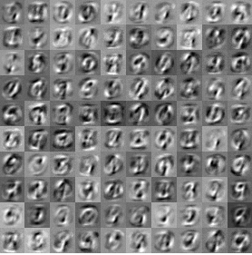
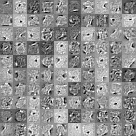
Figure 1: $100$ MNIST feature weights (one image per hidden unit) learned by Probit RBM (left) and RBM with CD-1 (right).

We report here the result of the mean-field method for computing data-dependent statistics, which are averaged over a random batch of $500$ images. For the data-independent statistics, $500$ persistent chains are run in parallel with samples collected after every $5$ Gibbs steps. The sparsity level $\rho$ is set to $0.3$ and the sparseness weight $\lambda$ is set to $0.5$. Once the model has been learned, mean-field is used to estimate the hidden posteriors. Typically this mean-field is quite fast as it converges in a few steps.

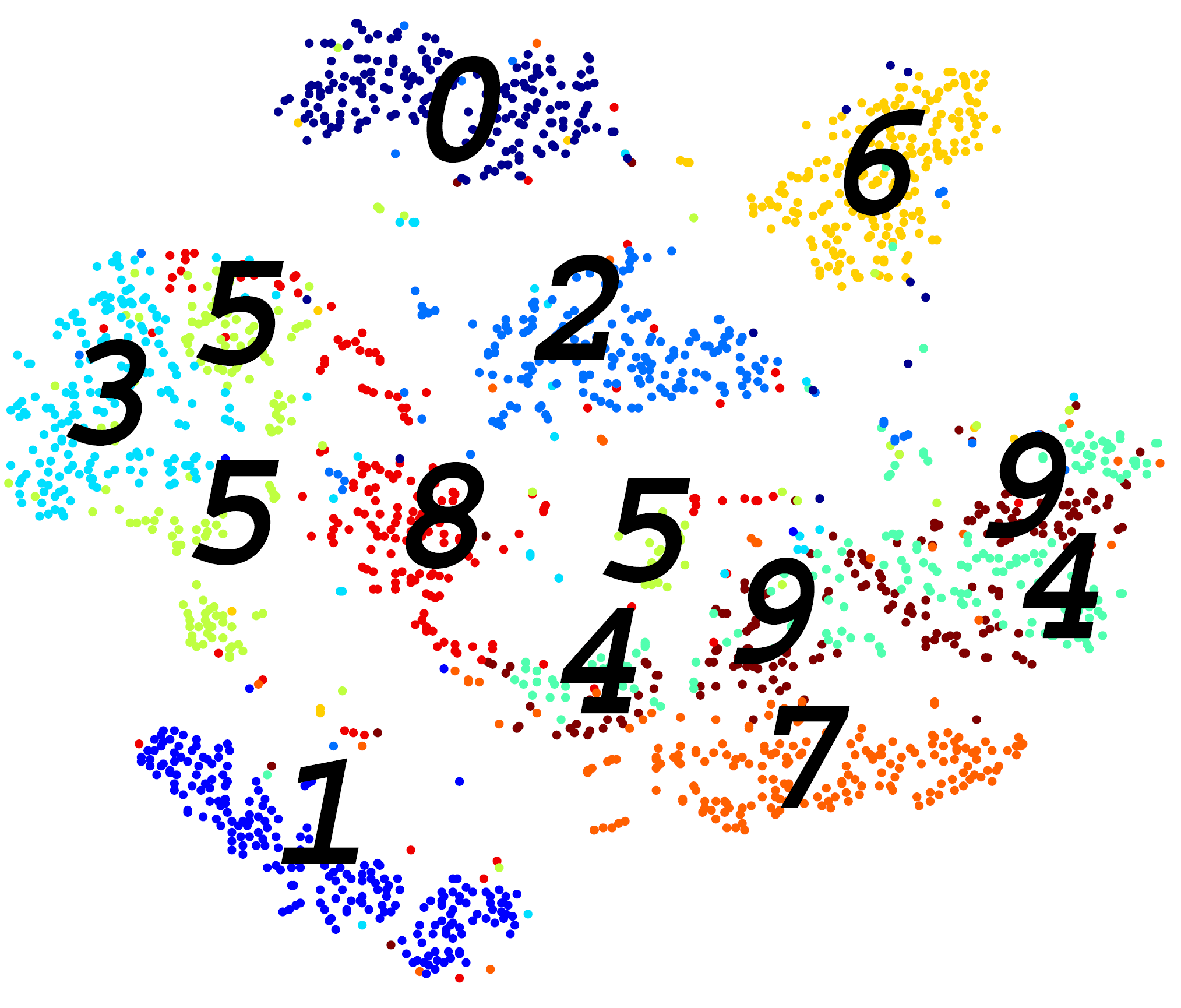
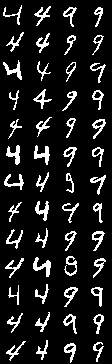
Figure 2: t-SNE visualisation of the learned representations on MNIST (left) and random samples of two confused digits (4,9) (right). Best viewed in colours.

We take the data from MNIST and binarize the images using a mid-intensity threshold. The learned representation is shown in Figure 2. Most digits are well separated in 2D except for digits $4$ and $9$. The learned representation can be used for classifications, e.g., by feeding to the multiclass logistic classifier. For $500$ hidden units, the Probit RBM achieves the error rate of $3.28$%, comparable with those obtained by the RBM trained with CD-$1$ ($3.02$%), and much better than the raw pixels ($8.46$%). The features discovered by the Probit RBM and RBM with CD-$1$ are very different (Figure 1), and this is expected because they operate on different input representations. The energy surface learned by the Probit RBM is smooth enough to allow efficient exploration of modes, as shown in Figure 3.

      

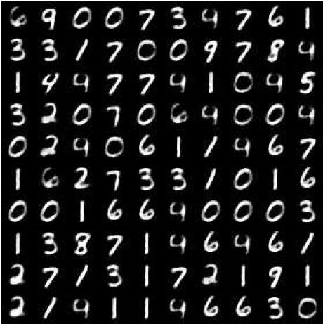
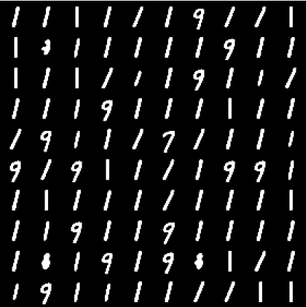
Figure 3: Samples generated from the Probit RBM (left) and RBM with CD-1 (right) by mode seeking procedures (see Supplement).

6.2 Rank Evidences for Collaborative Filtering

In collaborative filtering, one of the main goals is to produce a personalized ranked list of items. Until very recently, the majority in the area, on the other hand, focused on predicting the ratings, which are then used for ranking items. It can be arguably more efficient to learn a rank model directly instead of going through the intermediate steps.

We build one $\mathrm{TBM}$ for ranking with ties (i.e., inequality constraints, see Section 3.2) per user due to the variation in item choices but all the $\mathrm{TBM}$s share the same parameter set. The handling of ties is necessary because during training, many items share the same rating. Unseen items are simply not accounted for in each model: We only need to compare the utilities between the items seen by each person. The result is that the models are very sparse and fast to run. For the data-dependent statistics, we maintain one Markov chain per user. Since there is no single model for all data instances, the data-independent statistics cannot be estimated from a small set of Markov chains. Rather we also maintain a data-independent chain per data instance, which can be persistent on their own, or restarted from the data-dependent chains after every parameter updating step. The latter case, which is reported here, is in the spirit of the Hinton’s Contrastive Divergence, where the data-independent chain is just a few steps away from the data-dependent chain.

Once the model has been trained, the hidden posterior vector $\hat{\boldsymbol{h}}=\left(\hat{h}_{1},\hat{h}_{2},...,\hat{h}_{K}\right)$, where $\hat{h}_{k}=P(h_{k}=1\mid\boldsymbol{e}_{u})$, is used as the new representation of the tastes of user $u$. The rank of unseen movies is the mode of the distribution $P(\boldsymbol{e}^{*}\mid\hat{\boldsymbol{h}})$, where $\boldsymbol{e}^{*}$ are the rank-based evidences (see Section 4.4). For fast computation of $P(\boldsymbol{e}^{*}\mid\hat{\boldsymbol{h}})$, we approximate the Gaussian by a Gumbel distribution, which leads to a simple way of ranking movies using the mean “utility” $\mu_{ui}=\alpha_{i}+W_{i\bullet}\hat{\boldsymbol{h}}_{u}$ for user $u$ (see the Supplement for more details).

The data used in this experiment is the MovieLens, which contains $1$M ratings by approximately $6$K users on $4$K movies. To encourage diversity in the rank lists, we remove the top $10$% most popular movies. We then remove users with less than $30$ ratings on the remaining movies. The most recently rated $10$ movies per user are held out for testing, the next most recent $5$ movies are used for tuning hyper-parameters, and the rest for training.

For comparison, we implement a simple baseline using item popularity for ranking, and thus offering a naive non-personalized solution. For personalized alternatives, we implement two recent rank-based matrix factorisation methods, namely ListRank.MF [27] and PMOP [36]. Two ranking metrics from the information retrieval literature are used: the ERR [3] and the NDCG@T [13]. These metrics place more emphasis on the top-ranked items. Table 1 reports the movie ranking results on test subset (each user is presented with a ranked list of unseen movies), demonstrating that the $\mathrm{TBM}$ is a clear winner in all metrics.

	ERR	N@1	N@5	N@10
Item popularity	0.587	0.560	0.680	0.835
ListRank.MF	0.653	0.673	0.751	0.873
PMOP	0.648	0.664	0.747	0.871
$\mathrm{TBM}$	0.678	0.722	0.792	0.893

Table 1: Item ranking results on MovieLens – the higher the better ($K=50$). Here N@T is a shorthand for NDCG@T.

6.3 Mixed Evidences for World Attitude Analysis

Finally, we demonstrate the $\mathrm{TBM}$ on mixed evidences. The data is from the survey analysis domain, which mostly consists of multiple questions of different natures such as basic facts (e.g., ages and genders) and opinions (e.g., binary choices, single choices, multiple choices, ordinal judgments, preferences and ranks). The standard approach to deal with such heterogeneity is to perform the so-called “coding”, which converts types into some numerical representations (e.g., ordinal scales into stars, ranks into multiple pairwise comparisons) so that standard processing tools can handle. However, this coding process breaks the structure in the data and thus significant information will be lost. Thus our $\mathrm{TBM}$ offers a scalable and generic machinery to process the data in its native format and then convert the mixed types into a more homogeneous posterior vector.

We use the global attitude survey dataset collected by the PewResearch Centre. The survey was conducted on $24,717$ people from $24$ countries during the period of March 17 – April 21, 2008 on a variety of topics concerning people’s life, opinions on issues in their countries and around the world as well as future expectations. There are $52$ binary, $124$ categorical (of variable category sizes), $3$ continuous, $165$ ordinal (of variable level sizes) question types.

Like the case of collaborative filtering, we build one $\mathrm{TBM}$ per respondent due to the variation in questions and answers but all the $\mathrm{TBM}$s share the same parameter set. Unanswered/inappropriate questions are ignored. For each respondent, we maintain $2$ persistent and non-interacting Markov chains for the data-dependent statistics and the data-independent statistics, respectively.

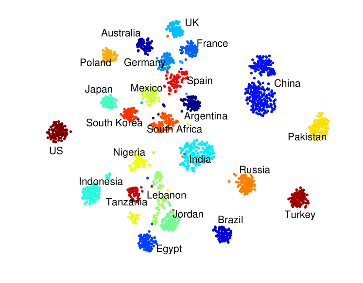
Figure 4: Distribution of global attitudes obtained by projecting the hidden posteriors ($100$ hidden units) on 2D using t-SNE. A dot represents one respondent. Best viewed in colours.

Figure 4 shows the 2D distribution of respondents from $24$ countries obtained by feeding the posteriors to the t-SNE [38] (here no explicit information of countries is used). It is interesting to see the cultural/social clustering and gaps between countries as opposed to the geographical distribution (e.g., between Indonesia and Egypt, Australia and UK and the relative separation of the China, Pakistan, Turkey and the US from the rest). To predict the $24$ countries, we feed the posteriors into the standard multiclass logistic regression and achieve an error rate of $0.49\%$, suggesting that the $\mathrm{TBM}$ has captured the intrastate regularities and separated the interstate variations well.

7 Related Work

Latent multivariate Gaussian variables have been widely studied in statistical analysis, initially to model correlated binary data [1, 4] then now used for a variety of data types such as ordered categories [15], unordered categories [43], and the mixture of types [6]. Learning with the underlying Gaussian model is notoriously difficult for large-scale setting: independent sampling costs cubic time due to the need of inverting the covariance matrix, while MCMC techniques such as Gibbs sampling can be very slow if the graph is dense and the interactions between variables are strong. This can be partly overcome by adding one more layer of latent variables as in factor analysis [39, 14] and probabilistic principle component analysis [33]. The main difference from our $\mathrm{TBM}$ is that those models are directed with continuous factors while ours is undirected with binary factors.

Gaussian RBMs have been used for modelling continuous data such as visual features [12], where the evidences are the value assignments, and thus a limiting case of our evidence system. Some restrictions to the continuous Boltzmann machines have been studied: In [5], Gaussian variables are assumed to be non-negative, and in [41], continuous variables are bounded. However, we do not make these restrictions on the model but rather placing restrictions during the training phase only. GRBMs that handle ordinal evidences have been studied in [35], which is an instance of the boxed-constraints in our $\mathrm{TBM}$.

8 Discussion and Conclusion

Since the underlying variables of the $\mathrm{TBM}$ are Gaussian, various extensions can be made without much difficulty. For example, direct correlations among variables, regardless of their types, can be readily modelled by introducing the non-identity covariance matrix [22]. This is clearly a good choice for image modelling since nearby pixels are strongly correlated. Another situation is when the input units are associated with their own attributes. Each unit can be extended naturally by adding a linear combination of attributes to the mean structure of the Gaussian.

The additive nature of the mean-structure allows the natural extension to matrix modelling (e.g., see [37, 35]). That is, we do not distinguish the role of rows and columns, and thus each row and column can be modelled using their own hidden units (the row parameters and columns parameters are different). Conditioned on the row-based hidden units, we return to the standard $\mathrm{TBM}$ for column vectors. Inversely, conditioned on the column-based hidden units, we have the $\mathrm{TBM}$ for row vectors.

To sum up, we have proposed a generic class of models called Thurstonian Boltzmann machine ($\mathrm{TBM}$) to unify many type-specific modelling problems and generalise them to the general problem of learning from multiple groups of inequalities. Our framework utilises the Gaussian restricted Boltzmann machines, but the Gaussian variables are never observed except for one limiting case. Rather, those variables are subject to inequality constraints whenever an evidence is observed. Under this representation, the $\mathrm{TBM}$ supports a very wide range of evidences, many of which were not possible before in the Boltzmann machine literature, without the need to specify type-specific models. In particular, the $\mathrm{TBM}$ supports any combination of the point assignments, intervals, censored values, binary, unordered categories, multi-categories, ordered categories, (in)-complete ranks with and without ties.

We demonstrated the $\mathrm{TBM}$ on three applications of very different natures, namely handwritten digit recognition, collaborative filtering and complex survey analysis. The results are satisfying and the performance is competitive with those obtained by type-specific models.

Appendix A Supplementary Material

A.1 Inference

A.1.1 Estimating the Partition Function

For convenience, let us re-parameterise the distribution as follows

$$\phi_{i}(x_{i}) = \exp\left\{-\frac{x_{i}^{2}}{2}+\alpha_{i}x_{i}\right\}$$ (9)

$$\psi_{ik}(x_{i},h_{k}) = \exp\left\{W_{ik}x_{i}h_{k}\right\}$$

$$\phi_{k}(h_{k}) = \exp\left\{\gamma_{k}h_{k}\right\}$$

The model potential is then the product of all local potentials

$$\Psi(\boldsymbol{x},\boldsymbol{h})=\left[\prod_{i}\phi_{i}(x_{i})\right]\left[\prod_{ik}\psi_{ik}(x_{i},h_{k})\right]\left[\prod_{k}\phi_{k}(h_{k})\right]$$ (10)

The partition function can be rewritten as

$$Z = \sum_{\boldsymbol{h}}\int_{\boldsymbol{x}}\Psi(\boldsymbol{x},\boldsymbol{h})d\boldsymbol{x}$$

$$= \sum_{\boldsymbol{h}}\Omega(\boldsymbol{h})$$

where $\Omega(\boldsymbol{h})=\int_{\boldsymbol{x}}\Psi(\boldsymbol{x},\boldsymbol{h})d\boldsymbol{x}$. We now proceed to compute $\Omega(\boldsymbol{h})$:

$$\Omega(\boldsymbol{h}) = \left[\prod_{k}\phi_{k}(h_{k})\right]\int_{\boldsymbol{x}}\left[\prod_{i}\phi_{i}(x_{i})\right]\left[\prod_{ik}\psi_{ik}(x_{i},h_{k})\right]d\boldsymbol{x}$$

$$= \left[\prod_{k}\phi_{k}(h_{k})\right]\prod_{i}\int_{x_{i}}\exp\left\{-\frac{x_{i}^{2}}{2}+(\alpha_{i}+\sum_{k}W_{ik}h_{k})x_{i}\right\}dx_{i}$$

$$= \left[\prod_{k}\phi_{k}(h_{k})\right]\prod_{i}C_{i}\int_{x_{i}}\exp\left\{-\frac{\left(x_{i}-\mu_{i}(\boldsymbol{h})\right)^{2}}{2}\right\}dx_{i}$$

$$= \left[\prod_{k}\phi_{k}(h_{k})\right]\prod_{i}C_{i}\sqrt{2\pi\sigma_{i}^{2}}$$

where

$$\mu_{i}(\boldsymbol{h}) = \alpha_{id}+\sum_{k=1}^{K}W_{ik}h_{k}$$

$$C_{i} = \exp\left\{\frac{1}{2}\left(\frac{\mu_{i}(\boldsymbol{h})}{\sigma_{i}}\right)^{2}\right\}$$

Now we can define the distribution over the hidden layer as follows

$$P(\boldsymbol{h})=\frac{1}{Z}\Omega(\boldsymbol{h})$$

Now we apply the Annealed Importance Sampling (AIS) [19]. The idea is to introduces the notion of inverse-temperature $\tau$ into the model, i.e., $P(\boldsymbol{h}|\tau)\propto\Omega(\boldsymbol{h})^{\tau}$.

Let $\{\tau_{s}\}_{s=0}^{S}$ be the (slowly) increasing sequence of temperature, where $\tau_{0}=0$ and $\tau_{S}=1$, that is $\tau_{0}<\tau_{1}...<\tau_{S}$. At $\tau_{0}=0$, we have a uniform distribution, and at $\tau_{S}=1$, we obtain the desired distribution. At each step $s$, we draw a sample $\boldsymbol{h}^{s}$ from the distribution $P(\boldsymbol{h}|\tau_{s-1})$ (e.g. using some Metropolis-Hastings procedure). Let $P^{*}(\boldsymbol{h}|\tau)$ be the unnormalised distribution of $P(\boldsymbol{h}|\tau)$, that is $P(\boldsymbol{h}|\tau)=P^{*}(\boldsymbol{h}|\tau)/Z(\tau)$. The final weight after the annealing process is computed as

$$\omega =\frac{P^{*}(\boldsymbol{h}^{1}|\tau_{1})}{P^{*}(\boldsymbol{h}^{1}|\tau_{0})}\frac{P^{*}(\boldsymbol{h}^{2}|\tau_{2})}{P^{*}(\boldsymbol{h}^{2}|\tau_{1})}...\frac{P^{*}(\boldsymbol{h}^{S}|\tau_{S})}{P^{*}(\boldsymbol{h}^{S}|\tau_{S-1})}$$

The above procedure is repeated $T$ times. Finally, the normalisation constant at $\tau=1$ is computed as $Z(1)\approx Z(0)\left(\sum_{t=1}^{T}\omega^{(t)}/T\right)$ where $Z(0)=2^{K}$, which is the number of configurations of the hidden variables $\boldsymbol{h}$.

A.1.2 Estimating Posteriors using Mean-field

Recall that for evidence $\boldsymbol{e}$ we want to estimate posteriors $P(\boldsymbol{h}\mid\boldsymbol{e})=\sum_{\boldsymbol{x}\in\Omega(\boldsymbol{e})}P_{\Omega(\boldsymbol{e})}(\boldsymbol{h},\boldsymbol{x}\mid\boldsymbol{e})$. Assume that the evidences can be expressed in term of boxed constraints, which lead to the following factorisation

$$P(\boldsymbol{x}\mid\boldsymbol{e},\boldsymbol{h})=\prod_{i}P(x_{i}\mid\boldsymbol{e},\boldsymbol{h})$$

This factorisation is critical because it ensures that there are no deterministic constraints among $\left\{x_{i}\right\}_{i=1}^{n}$, which are the conditions that variational methods such as mean-fields would work well. This is because mean-field solution will generally not satisfy deterministic constraints, and thus may assign non-zeros probability to improbably areas.

To be more concrete, the mean-field approximation would be $Q(\boldsymbol{h},\boldsymbol{x})\approx P(\boldsymbol{h},\boldsymbol{x}\mid\boldsymbol{e})$

$$Q(\boldsymbol{h},\boldsymbol{x}) = \prod_{k}Q_{k}(h_{k})\prod_{i}Q_{i}(x_{i})$$

$$\mbox{s.t.}\quad\boldsymbol{x} \in \Omega(\boldsymbol{e})$$

The best mean-field approximation will be the minimiser of the Kullback-Leibler divergence

$$\mathcal{D}\left(Q||P\right) = \sum_{\boldsymbol{h}}\sum_{\boldsymbol{x}\in\Omega(\boldsymbol{e})}Q(\boldsymbol{h},\boldsymbol{x})\log\frac{Q(\boldsymbol{h},\boldsymbol{x})}{P(\boldsymbol{h},\boldsymbol{x}\mid\boldsymbol{e})}$$ (11)

$$= -H\left[Q(\boldsymbol{h},\boldsymbol{x})\right]-\sum_{\boldsymbol{h}}\sum_{\boldsymbol{x}\in\boldsymbol{\Omega}(\boldsymbol{e})}Q(\boldsymbol{h},\boldsymbol{x})\log P(\boldsymbol{h},\boldsymbol{x}\mid\boldsymbol{e})$$

where $H\left[Q(\boldsymbol{h},\boldsymbol{x})\right]$ is the entropy function. Now first, exploit the fact that $Q$ is factorisable, and thus its entropy is decomposable, i.e.,

$$H\left[Q(\boldsymbol{h},\boldsymbol{x})\right]=\sum_{k}H\left[Q_{k}(h_{k})\right]+\sum_{i}H\left[Q_{i}(x_{i})\right]$$ (12)

Second recall from Eq. (17) that

$$P(\boldsymbol{h},\boldsymbol{x}\mid\boldsymbol{e})=\frac{1}{Z(\boldsymbol{e})}\exp\left\{-E(\boldsymbol{x},\boldsymbol{h})\right\}$$

and thus

$$\sum_{\boldsymbol{h}}\sum_{\boldsymbol{x}\in\boldsymbol{\Omega}(\boldsymbol{e})}Q(\boldsymbol{h},\boldsymbol{x})\log P(\boldsymbol{h},\boldsymbol{x}\mid\boldsymbol{e})=-\sum_{\boldsymbol{h}}\sum_{\boldsymbol{x}\in\boldsymbol{\Omega}(\boldsymbol{e})}Q(\boldsymbol{h},\boldsymbol{x})E(\boldsymbol{x},\boldsymbol{h})-\log Z(\boldsymbol{e})$$

Since $\log Z(\boldsymbol{e})$ is a constraint w.r.t. $Q(\boldsymbol{h},\boldsymbol{x})$, we can safely ignore it here.

Now since $E(\boldsymbol{x},\boldsymbol{h})$ is decomposable (see Eq. (2)), we have

$$\sum_{\boldsymbol{h}}\sum_{\boldsymbol{x}\in\boldsymbol{\Omega}(\boldsymbol{e})}Q(\boldsymbol{h},\boldsymbol{x})E(\boldsymbol{x},\boldsymbol{h}) = \left(\sum_{i}\sum_{x_{i}\in\Omega(e_{i})}Q_{i}(x_{i})E_{i}(x_{i})\right)+\left(\sum_{k}\sum_{h_{k}}Q_{k}(h_{k})E_{k}(h_{k})\right)+$$

$$\quad+\left(\sum_{i}\sum_{k}\sum_{x_{i}\in\Omega(e_{i})}\sum_{h_{k}}Q_{i}(x_{i})Q_{k}(h_{k})E_{ik}(x_{i},h_{k})\right)$$

where

$$E_{i}(x_{i}) = \frac{x_{i}^{2}}{2}-\alpha_{i}x_{i}$$

$$E_{k}(h_{k}) = -\gamma_{k}h_{k}$$

$$E_{ik}(x_{i},h_{k}) = -W_{ik}x_{i}h_{k}$$

Combining this decomposition and Eq. (12), we have completely decomposed the Kullback-Leibler divergence in Eq. (11) into local terms:

$$\mathcal{D}\left(Q||P\right) = \sum_{i}\sum_{x_{i}\in\Omega(e_{i})}Q_{i}(x_{i})E_{i}(x_{i})+\sum_{k}\sum_{h_{k}}Q_{k}(h_{k})E_{k}(h_{k})+$$

$$+\left(\sum_{i}\sum_{k}\sum_{x_{i}\in\Omega(e_{i})}\sum_{h_{k}}Q_{i}(x_{i})Q_{k}(h_{k})E_{ik}(x_{i},h_{k})\right)-\sum_{i}H\left[Q_{i}(x_{i})\right]-\sum_{k}H\left[Q_{k}(h_{k})\right]$$

Now we wish to minimise the divergence with respect to the local distributions $\left\{Q_{i}(x_{i}),Q_{k}(h_{k})\right\}$ for $i=1,2,...,N$ and$k=1,2,...,K$ knowing the proper distribution constraints

$$\int_{x_{i}\in\Omega(e_{i})}Q_{i}(x_{i}) = 1$$

$$\sum_{h_{k}}Q_{k}(h_{k}) = 1$$

By the method of Lagrangian multiplier, we have

$$L(\lambda)=\mathcal{D}\left(Q||P\right)+\sum_{i}\lambda_{i}\left(\int_{x_{i}\in\Omega(e_{i})}Q_{i}(x_{i})-1\right)+\sum_{k}\kappa_{k}\left(\sum_{h_{k}}Q_{k}(h_{k})-1\right)$$

• Let us compute the partial derivative w.r.t. $Q_{i}(x_{i})$:

  $$\partial_{Q_{i}(x_{i})}L(\lambda) = \log Q_{i}(x_{i})+1+E_{i}(x_{i})+\sum_{k}Q_{k}(h_{k}^{1})E_{ik}(x_{i},h_{k}^{1})+\lambda_{i}$$

  where $h_{k}^{1}$ is a short hand for $h_{k}=1$ and we have made use of the fact that $E_{ik}(x_{i},h_{k}=0)=0$. Setting this gradient to zero yields

  $$Q_{i}(x_{i}) = \exp\left\{-\left(E_{i}(x_{i})+\sum_{k}Q_{k}(h_{k}^{1})E_{ik}(x_{i},h_{k}^{1})\right)-1-\lambda_{i}\right\}$$ (13)

  $$= \exp\left\{-\frac{1}{2}\left(x_{i}-\left(\alpha_{i}+\sum_{k}Q_{k}(h_{k}^{1})W_{ik}\right)\right)^{2}-1-\lambda_{i}\right\}$$

  for $x_{i}\in\Omega(e_{i})$. Normalising this distribution would lead to the truncated form of the normal distribution those the mean is

  $$\mu_{i}=\alpha_{i}+\sum_{k}Q_{k}(h_{k}^{1})W_{ik}h_{k}$$ (14)

• In a similar way, the partial derivative w.r.t. $Q_{k}(h_{k})$ would be

  $$\partial_{Q_{k}(h_{k})}L(\lambda)=\log Q_{k}(h_{k})-h_{k}\left(\gamma_{k}+\sum_{i}W_{ik}\sum_{x_{i}\in\Omega(e_{i})}Q_{i}(x_{i})x_{i}\right)+1+\kappa_{k}$$

  Equating the gradient to zero, we have

  $$Q_{k}(h_{k})\propto\exp\left\{h_{k}\left(\gamma_{k}+\sum_{i}W_{ik}\hat{\mu}_{i}\right)\right\}$$

  where $\hat{\mu}_{i}$ is the mean of the truncated normal distribution

  $$\hat{\mu}_{i}=\sum_{x_{i}\in\Omega(e_{i})}Q_{i}(x_{i})x_{i}$$

  Normalising $Q_{k}(h_{k})$ would lead to

  $$Q_{k}(h_{k}^{1})=\left[1+\exp\left\{-\gamma_{k}-\sum_{i}W_{ik}\hat{\mu}_{i}\right\}\right]^{-1}$$ (15)

• Finally, combining these findings in Eqs. (13,14,15), and letting $\Omega(e_{i})=[b_{i},c_{i}]$ be the boxed constraint, and using the fact that the mean of the truncated distribution is

  $$\hat{\mu}_{i}=\mu_{i}+\frac{\phi(b_{i}-\mu_{i})-\phi(c_{i}-\mu_{i})}{\Phi(c_{i}-\mu_{i})-\Phi(b_{i}-\mu_{i})}$$

  we would arrive at the three recursive equations

  $$q_{k} \leftarrow \frac{1}{1+\exp\left\{-\gamma_{k}-\sum_{i}W_{ik}\hat{\mu}_{i}\right\}}$$

  $$\mu_{i} \leftarrow \alpha_{i}+\sum_{k}W_{ik}q_{k}$$

  $$\hat{\mu}_{i} \leftarrow \mu_{i}+\frac{\phi(b_{i}-\mu_{i})-\phi(c_{i}-\mu_{i})}{\Phi(c_{i}-\mu_{i})-\Phi(b_{i}-\mu_{i})}$$

  where $q_{k}$ is a short hand for $Q_{k}(h_{k}^{1})$ and$\phi(z)$ is the normal probability density function, and $\Phi(z)$ is the cumulative distribution function $\clubsuit$

A.1.3 Seeking Modes and Generating Representative Samples

Once the model has been learned, samples can be generated straightforwardly by first sampling the underlying Gaussian RBM and then collect the true samples that satisfy the inequalities of interest. For example, for binary samples, if the generated Gaussian value for a visible unit is larger than the threshold, then we have an active sample. Likewise, rank samples, we only need to rank the sampled Gaussian values.

However, this may suffer from the poor mixing if we use standard Gibbs sampling, that is the Markov chain may get stuck in some energy traps. To jump out of the trap we propose to periodically raise the temperature to a certain level (e.g., $10$) and then slowly cool down to the original temperature (which is $1$). In our experiment, the cooling is scheduled as follows

$$T\leftarrow\eta T$$

where $\eta\in(0,1)$ is estimated so that for $n$ steps, the temperature will drop from $T_{max}$ to $T_{min}$. That is, $T_{min}=\eta^{n}T_{max}$, leading to $\eta=\left(T_{min}/T_{max}\right)^{1/n}$.

To locate a basis of attraction, we can lower the temperature further (e.g., to $0.1$) to trap the particles there. Then we collect $k$ successive samples and take the average to be the representative sample. In our experiments, $k=50$.

A.2 Learning

A.2.1 Gradient of the Likelihood

The log-likelihood of an evidence is

$$\mathcal{L} = \log P(\boldsymbol{e})=\log\sum_{\boldsymbol{h}}\int_{\boldsymbol{\Omega}(\boldsymbol{e})}P(\boldsymbol{h},\boldsymbol{x})d\boldsymbol{x}$$

$$= \log\sum_{\boldsymbol{h}}\int_{\boldsymbol{\Omega}(\boldsymbol{e})}\exp\left\{-E(\boldsymbol{x},\boldsymbol{h})\right\}d\boldsymbol{x}-\log Z$$

$$= \log Z(\boldsymbol{e})-\log Z$$

where $Z(\boldsymbol{e})=\sum_{\boldsymbol{h}}\int_{\boldsymbol{\Omega}(\boldsymbol{e})}\exp\left\{-E(\boldsymbol{x},\boldsymbol{h})\right\}d\boldsymbol{x}$. The gradient of $\log Z(\boldsymbol{e})$ w.r.t. the mapping parameter $W_{ik}$ reads

$$\partial_{W_{ik}}\log Z(\boldsymbol{e}) = \frac{-1}{Z(\boldsymbol{e})}\sum_{\boldsymbol{h}}\int_{\boldsymbol{\Omega}(\boldsymbol{e})}\exp\left\{-E(\boldsymbol{x},\boldsymbol{h})\right\}\partial_{W_{ik}}E(\boldsymbol{x},\boldsymbol{h})d\boldsymbol{x}$$ (16)

$$= -\sum_{\boldsymbol{h}}\int_{\boldsymbol{\Omega}(\boldsymbol{e})}P(\boldsymbol{x},\boldsymbol{h}\mid\boldsymbol{e})\partial_{W_{ik}}E(\boldsymbol{x},\boldsymbol{h})d\boldsymbol{x}$$

where we have moved the constant $Z^{-1}(\boldsymbol{e})$ into the sum and integration and make use of the fact that

$$P(\boldsymbol{x},\boldsymbol{h}\mid\boldsymbol{e})=\frac{P(\boldsymbol{x},\boldsymbol{h})}{P(\boldsymbol{e})}=\frac{1}{Z(\boldsymbol{e})}\exp\left\{-E(\boldsymbol{x},\boldsymbol{h})\right\}$$ (17)

where the domain of the Gaussian is constrained to $\boldsymbol{x}\in\boldsymbol{\Omega}(\boldsymbol{e})$.

From the definition of the energy function in Eq. (2), we know that the energy is decomposable, and thus the gradient w.r.t. $W_{ik}$ only involves the pair $(x_{i},h_{k})$. In particular

$$\partial_{W_{ik}}E(\boldsymbol{x},\boldsymbol{h})=-x_{i}h_{k}$$

This simplifies Eq. (16)

$$\partial_{W_{ik}}\log Z(\boldsymbol{e}) = -\sum_{h_{i}}\int_{\Omega(e_{i})}P(x_{i},h_{k}\mid\boldsymbol{e})\partial_{W_{ik}}E(\boldsymbol{x},\boldsymbol{h})dx_{i}$$

$$= \mathbb{E}_{P(\boldsymbol{x},\boldsymbol{h}\mid\boldsymbol{e})}\left[x_{i}h_{k}\right]$$

A similar process would lead to

$$\partial_{W_{ik}}\log Z=\mathbb{E}_{P(x_{i},h_{k})}\left[x_{i}h_{k}\right]$$

and finally:

$$\partial_{W_{ik}}\mathcal{L} = \mathbb{E}_{P(x_{i},h_{k}\mid\boldsymbol{e})}\left[x_{i}h_{k}\right]-\mathbb{E}_{P(x_{i},h_{k})}\left[x_{i}h_{k}\right]\clubsuit$$

A.2.2 Regularising the Markov Chains

One undesirable feature of the MCMC chains used in learning we have experiences so far is the tendency for the binary hidden states to get stuck, i.e., after some point they do not flip their assignments as learning progresses. We conjecture that this phenomenon may be due to the saturation effect inherent in the factor posterior:

$$P(h_{k}=1\mid\boldsymbol{x})=\frac{1}{1+\exp\left(-\gamma_{k}-\sum_{i}W_{ik}x_{i}\right)}$$

i.e., once the collected value to a node $\left(\gamma_{k}+\sum_{i}W_{ik}x_{i}\right)$ is too high or too low, it is very hard to over turn.

Fortunately, there is a known technique to regularise the chain: we enforce that at a time, there should be only a fraction $\rho$ of nodes which are active, where $\rho\in(0,1)$. One way is to maximise the following objective function

$$\mathcal{L}_{2} = \mathcal{L}+\lambda\int\left[\sum_{k}\sum_{h_{k}}\rho(h_{k})\log P(h_{k}\mid\boldsymbol{x})\right]P(\boldsymbol{x}\mid\boldsymbol{e})d\boldsymbol{x}$$

where $\lambda>0$ is the weighting factor, $\rho(h_{k})=\rho$ if $h_{k}=1$ and $\rho(h_{k})=1-\rho$ otherwise.

The gradient with respect to $g_{k}=\left(\gamma_{k}+\sum_{i}W_{ik}x_{i}\right)$ is then

$$\partial_{g_{k}}\mathcal{L}_{2} = \partial_{g_{k}}\mathcal{L}+\lambda\int\left[\partial_{g_{k}}\sum_{h_{k}}\rho(h_{k})\log P(h_{k}\mid\boldsymbol{x})\right]P(\boldsymbol{x}|\boldsymbol{e})d\boldsymbol{x}$$

$$= \partial_{g_{k}}\mathcal{L}+\lambda\int\left[\rho-P(h_{k}^{1}\mid\boldsymbol{x})\right]P(\boldsymbol{x}|\boldsymbol{e})d\boldsymbol{x}$$

$$\approx \partial_{g_{k}}\mathcal{L}+\frac{1}{S}\lambda\sum_{s}\left[\rho-P(h_{k}^{1}\mid\boldsymbol{x}^{(s)})\right]$$

where $S$ is the number of samples and $P(h_{k}^{1}\mid\boldsymbol{x})$ is a shorthand for $P(h_{k}=1\mid\boldsymbol{x})$. Using the chain rule, we have:

$$\partial_{\gamma_{k}}\mathcal{L}_{2} \approx \partial_{\gamma_{k}}\mathcal{L}+\frac{1}{S}\lambda\sum_{s}\left[\rho-P(h_{k}^{1}\mid\boldsymbol{x}^{(s)})\right]$$

$$\partial_{W_{ik}}\mathcal{L}_{2} \approx \partial_{w_{ikd}}\mathcal{L}+\frac{1}{S}\lambda\sum_{s}x_{i}\left[\rho-P(h_{k}^{1}\mid\boldsymbol{x}^{(s)})\right]$$

A.2.3 Online Estimation of Posteriors

For tasks such as data completion (e.g., collaborative filtering) we need the posteriors $P(\boldsymbol{h}\mid\boldsymbol{e})$ for the prediction phase. One way is to run the Markov chain or doing mean-field from scratch. Here we suggest a simple way to obtain an approximation directly from the training phase without any further cost. The idea is to update the estimated posterior $\hat{\boldsymbol{h}}$ at each learning step $t$ in an exponential smoothing fashion:

$$\hat{\boldsymbol{h}}^{(t)}\leftarrow\eta\hat{\boldsymbol{h}}^{(t-1)}+(1-\eta)\hat{\boldsymbol{h}}^{(t)}$$

for some smoothing factor $\eta\in(0,1)$ and initial $\hat{\boldsymbol{h}}^{(0)}$, where $\bar{h}_{k}^{(t)}=P(h_{k}^{1}\mid\boldsymbol{x}^{(t)},\boldsymbol{e})$ and $\boldsymbol{x}^{(t)}$ is the sampled Gaussian at time $t$.

As learning progresses, early samples, which are from incorrect models, will be exponentially weighted down. Typically we choose $\eta$ close to $1$, e.g., $\eta=0.9$.

A.2.4 Monitoring the Learning Progress

It is often of practical importance to track the learning progress, either by the reconstruction errors or by the data likelihood. The data likelihood can be estimated as

$$P(\boldsymbol{e})\approx\frac{1}{S}\sum_{s=1}^{S}\int_{\boldsymbol{\Omega}(\boldsymbol{e})}P(\boldsymbol{x}\mid\boldsymbol{h}^{(s)})d\boldsymbol{x}$$

where $\boldsymbol{h}^{(s)}$ are those samples collected as learning progressed in the data-independent phase, and the integration can be carried out using the technique described in the main text.

A.3 Extreme Value Distributions

Extreme value distributions are a class of distributions of extremal measurements [11]. Here we are concerned about the popular Gumbel’s distribution.

A.3.1 Gumbel Distribution for Categorical Choices

Let us start from the Gumbel density function

$$P(x)=\frac{1}{\sigma}\exp\left\{-\left(\frac{x-\mu}{\sigma}+e^{-\frac{x-\mu}{\sigma}}\right)\right\}$$

where $\mu$ is the mode (location) and $\sigma$ is the scale parameter.

Using Laplace’s approximation (e.g., via Taylor’s expansion of $\left(\frac{x-\mu}{\sigma}+e^{-\frac{x-\mu}{\sigma}}\right)$ using the second-order polynomial around $\mu$), we have

$$P(x)\propto\frac{1}{e\sigma}\exp\left\{-\frac{(x-\mu)^{2}}{2\sigma^{2}}\right\}$$

Renormalising this distribution, e.g., by replacing $e\approx 2.7183$ by $\sqrt{2\pi}\approx 2.5066$ we obtain the standard Gaussian distribution. Thus, we can use the Gumbel as an approximation to the Gaussian distribution.

Now we turn to the categorical model using Gumbel variables. We maintain one variable per category, which plays the role of the utility for the category. Assume that all utilities share the same scale parameter $\sigma$. The existing literature [18] asserts that the probability of choosing the $m$-th category is

$$P(e=c_{m})=\frac{e^{\mu_{m}/\sigma}}{\sum_{l}e^{\mu_{l}/\sigma}}$$

where $\mu_{l}$ is the location of the $l$-th utility.

When we choose a the $m$-th category we must ensure that $x_{m}>\max_{l\neq m}x_{l}$.

Let $y_{l}=\exp\left(-\frac{x_{l}-\mu_{l}}{\sigma}\right)$ or equivalently $x_{l}=\mu_{l}-\sigma\log y_{l}$. Thus $x_{l}<x_{m}$ means $\mu_{l}-\sigma\log y_{l}<\mu_{m}-\sigma\log y_{m}$, or $y_{l}>y_{m}\exp\left(\frac{\mu_{l}-\mu_{m}}{\sigma}\right)$.

The CDF of the $l$-th Gumbel distribution is

$$F_{l}(x_{m}) = \exp\left(-e^{-\frac{x_{m}-\mu_{l}}{\sigma}}\right)$$

$$= \exp\left(-e^{-\frac{x_{m}-\mu_{m}}{\sigma}}e^{\frac{\mu_{l}-\mu_{m}}{\sigma}}\right)$$

$$= \exp\left(-y_{m}e^{\frac{\mu_{l}-\mu_{m}}{\sigma}}\right)$$

Thus choosing category $c_{m}$ would mean

$$P(e=c_{m}) = \int P(x_{m})\left(\prod_{l\neq m}\int^{xm}P(x_{l})dx_{l}\right)dx_{m}$$

$$= \int P(x_{m})\prod_{l\neq m}F_{l}(x_{m})dx_{m}$$

We rewrite the Gumbel density function by changing variable from $x_{m}$ to $y_{m}$:

$$P(y_{m})=\frac{1}{\sigma}y_{m}\exp\left\{-y_{m}\right\}$$

for $y_{m}\geq 0$. Thus

$$P(x_{m})\prod_{l\neq m}F_{l}(x_{m})=\frac{1}{\sigma}y_{m}\exp\left(-y_{m}\left\{1+\sum_{l\neq m}e^{\frac{\mu_{l}-\mu_{m}}{\sigma}}\right\}\right)$$

Now, by changing variable under the integration from $x_{m}$ to $y_{m}$, we have

$$P(e=c_{m}) = \sigma\int_{0}^{\infty}P(y_{m})\prod_{l\neq m}F_{l}(y_{m})\frac{1}{y_{l}}dy_{m}$$

$$= \int_{0}^{\infty}\exp\left(-y_{m}\left\{1+\sum_{l\neq m}e^{\frac{\mu_{l}-\mu_{m}}{\sigma}}\right\}\right)dy_{m}$$

$$= \frac{1}{1+\sum_{l\neq m}e^{\frac{\mu_{l}-\mu_{m}}{\sigma}}}$$

$$= \frac{e^{\mu_{m}/\sigma}}{\sum_{l}e^{\mu_{l}/\sigma}}$$

A.3.2 Gumbel Distribution for Rank

We now extend the case of categorical evidences rank evidences. Again we maintain one Gaussian variable per category. Without loss of generality, for a particular rank $\pi$ we assume that we must ensure that $x_{1}>x_{2}>...>x_{D}$. This is equivalent to

$$\left[x_{1}>\max_{l>1}x_{l}\right]\cap\left[x_{2}>\max_{l>2}x_{l}\right]\cap...\cap\left[x_{D-1}>x_{D}\right]$$

The probability of this is essentially

$$P\left(\left\{e_{m}=m\right\}_{m=1}^{D}\right)=P(e_{1}=1)\prod_{m>2}P\left(e_{l}=m\mid\left\{e_{d}=l\right\}_{l=1}^{m-1}\right)$$

In words, this offers a stagewise process to rank categories: first we pick the best category, the pick the second best from the remaining categories and so on (see also [7]).

The probability of picking the best category out of a subset is already given in Appendix A.3.1:

$$P(e_{1}=1) = \frac{e^{\mu_{1}/\sigma}}{\sum_{l\geq 1}e^{\mu_{l}/\sigma}}$$

$$P\left(e_{l}=m\mid\left\{e_{d}=l\right\}_{l=1}^{m-1}\right) = \frac{e^{\mu_{m}/\sigma}}{\sum_{l\geq m}e^{\mu_{l}/\sigma}}$$

This gives us the Plackett-Luce model [17, 21] as mentioned in [30].

A.4 Global Attitude: Sample Questions

• Q4 (Ordinal): […] how would you describe the current economic situation in (survey country) – {very good, somewhat good, somewhat bad, or very bad}?

• Q11a (Binary): How do you think people in other countries of the world feel about China? – {like, disliked}?

• Q35,35a (Category-ranking): Which one of the following, if any, is hurting the world’s environment the most/second-most {India, Germany, China, Brazil, Japan, United States, Russia, Other}?

• Q76 (Continuous): How old were you at your last birthday?

• Q85 (Categorical): What is your current employment situation {A list of employment categories}?

A.5 Other Supporting Materials

A.5.1 Laplace Approximation

Laplace approximation is the technique using a Gaussian distribution to approximate another distribution. For the univariate case, assume that the original density distribution has the form

$$P(x)\propto\exp\left\{-f(x)\right\}$$

First we find the mode $\mu$ of $P(x)$ or equivalently the minimiser of $f(x)$ given it exists. Then we apply Taylor’s expansion

$$f(x)\approx f(\mu)+f^{\prime\prime}(\mu)\frac{\left(x-\mu\right)^{2}}{2}$$

The Gaussian approximation has the form

$$P^{*}(x)\propto\exp\left\{-f^{\prime\prime}(\mu)\frac{\left(x-\mu\right)^{2}}{2}\right\}$$

where $1/f^{\prime\prime}(\mu)$ is the new variance.

A.5.2 Some Properties of the Truncated Normal Distribution

For a normal distribution $P(x|\mu,\sigma)$ of mean $\mu$ and standard deviation $\sigma$ truncated from both sides, i.e., $\alpha<x<\beta$, the new density reads

$$\bar{P}_{[\alpha,\beta]}(x\mid,\mu,\sigma)=\frac{Q(x^{*})}{\sigma\left[\Phi(\beta^{*})-\Phi(\alpha^{*})\right]}$$

where

$$x^{*} = \frac{x-\mu}{\sigma};\quad\alpha^{*}=\frac{\alpha-\mu}{\sigma};\quad\beta^{*}=\frac{\beta-\mu}{\sigma}$$

and $Q(\cdot)$ and $\Phi(\cdot)$ are the probability density function and the cumulative distribution of the standard normal distribution, respectively. In particular, we are interested in the mean of the distribution $\bar{P}_{[\alpha,\beta]}$:

$$\bar{\mu}=\mu_{i}+\sigma\frac{Q(\alpha^{*})-Q(\beta^{*})}{\Phi(\beta^{*})-\Phi(\alpha^{*})}$$

Some special cases:

• When $\alpha=\beta$, this distribution reduces to the Dirac’s delta.

• When $\alpha=-\infty$, we have a one-sided truncation from above since $\Phi(\alpha^{*})=0$.

• When $\beta=+\infty$, we obtain a one-sided truncation form below since $\Phi(\beta^{*})=0$.

References

- [1] JR Ashford and RR Sowden. Multi-variate probit analysis. Biometrics, pages 535–546, 1970.
- [2] U. Böckenholt. Thurstonian-based analyses: past, present, and future utilities. Psychometrika, 71(4):615–629, 2006.
- [3] O. Chapelle, D. Metlzer, Y. Zhang, and P. Grinspan. Expected reciprocal rank for graded relevance. In CIKM, pages 621–630. ACM, 2009.
- [4] S. Chib and E. Greenberg. Analysis of multivariate probit models. Biometrika, 85(2):347–361, 1998.
- [5] O.B. Downs, D.J.C. MacKay, and D.D. Lee. The nonnegative Boltzmann machine. Advances in Neural Information Processing Systems, 12:428–434, 2000.
- [6] D.B. Dunson and A.H. Herring. Bayesian latent variable models for mixed discrete outcomes. Biostatistics, 6(1):11, 2005.
- [7] M.A. Fligner and J.S. Verducci. Multistage ranking models. Journal of the American Statistical Association, 83(403):892–901, 1988.
- [8] Y. Freund and D. Haussler. Unsupervised learning of distributions on binary vectors using two layer networks. Advances in Neural Information Processing Systems, pages 912–919, 1993.
- [9] P.V. Gehler, A.D. Holub, and M. Welling. The rate adapting Poisson model for information retrieval and object recognition. In Proceedings of the ICML, pages 337–344, 2006.
- [10] J. Geweke. Efficient simulation from the multivariate normal and student-t distributions subject to linear constraints and the evaluation of constraint probabilities. In Computing science and statistics: Proceedings of the 23rd symposium on the interface, pages 571–578, 1991.
- [11] EJ Gumbel. Statistical of extremes. Columbia University Press, New York, 1958.
- [12] G.E. Hinton and R.R. Salakhutdinov. Reducing the dimensionality of data with neural networks. Science, 313(5786):504–507, 2006.
- [13] K. Järvelin and J. Kekäläinen. Cumulated gain-based evaluation of IR techniques. ACM Transactions on Information Systems (TOIS), 20(4):446, 2002.
- [14] E. Khan, B. Marlin, and K. Murphy. Variational bounds for mixed-data factor analysis. In Proc. of Neural Information Processing Systems, 2010.
- [15] A. Kottas, P. Müller, and F. Quintana. Nonparametric Bayesian modeling for multivariate ordinal data. Journal of Computational and Graphical Statistics, 14(3):610–625, 2005.
- [16] N. Le Roux, N. Heess, J. Shotton, and J. Winn. Learning a generative model of images by factoring appearance and shape. Neural Computation, 23(3):593–650, 2011.
- [17] R.D. Luce. Individual choice behavior. Wiley New York, 1959.
- [18] D. McFadden. Conditional logit analysis of qualitative choice behavior. Frontiers in Econometrics, pages 105–142, 1973.
- [19] R.M. Neal. Annealed importance sampling. Statistics and Computing, 11(2):125–139, 2001.
- [20] J. Ngiam, A. Khosla, M. Kim, J. Nam, H. Lee, and A.Y. Ng. Multimodal deep learning. In ICML, 2011.
- [21] R.L. Plackett. The analysis of permutations. Applied Statistics, pages 193–202, 1975.
- [22] M.A. Ranzato and G.E. Hinton. Modeling pixel means and covariances using factorized third-order Boltzmann machines. In CVPR, pages 2551–2558. IEEE, 2010.
- [23] C.P. Robert. Simulation of truncated normal variables. Statistics and computing, 5(2):121–125, 1995.
- [24] R. Salakhutdinov and G. Hinton. Deep Boltzmann Machines. In Proceedings of 20th AISTATS, volume 5, pages 448–455, 2009.
- [25] R. Salakhutdinov and G. Hinton. Replicated softmax: an undirected topic model. Advances in Neural Information Processing Systems, 22, 2009.
- [26] R. Salakhutdinov, A. Mnih, and G. Hinton. Restricted Boltzmann machines for collaborative filtering. In Proceedings of the 24th ICML, pages 791–798, 2007.
- [27] Y. Shi, M. Larson, and A. Hanjalic. List-wise learning to rank with matrix factorization for collaborative filtering. In ACM RecSys, pages 269–272. ACM, 2010.
- [28] P. Smolensky. Information processing in dynamical systems: Foundations of harmony theory. Parallel distributed processing: Explorations in the microstructure of cognition, 1:194–281, 1986.
- [29] N. Srivastava and R. Salakhutdinov. Multimodal learning with deep Boltzmann machines. In NIPS, pages 2231–2239, 2012.
- [30] H. Stern. Models for distributions on permutations. Journal of the American Statistical Association, 85(410):558–564, 1990.
- [31] L.L. Thurstone. A law of comparative judgment. Psychological review, 34(4):273, 1927.
- [32] T. Tieleman. Training restricted Boltzmann machines using approximations to the likelihood gradient. In Proceedings of the 25th ICML, pages 1064–1071, 2008.
- [33] M.E. Tipping and C.M. Bishop. Probabilistic principal component analysis. Journal of the Royal Statistical Society: Series B, 61(3):611–622, 1999.
- [34] T. Tran, D.Q. Phung, and S. Venkatesh. Mixed-variate restricted Boltzmann machines. In Proc. of 3rd Asian Conference on Machine Learning (ACML), Taoyuan, Taiwan, 2011.
- [35] T. Tran, D.Q. Phung, and S. Venkatesh. Cumulative restricted Boltzmann machines for ordinal matrix data analysis. In Proc. of 4th Asian Conference on Machine Learning (ACML), Singapore, 2012.
- [36] T. Truyen, D.Q Phung, and S. Venkatesh. Probabilistic models over ordered partitions with applications in document ranking and collaborative filtering. In Proc. of SIAM Conference on Data Mining (SDM), Mesa, Arizona, USA, 2011. SIAM.
- [37] T.T. Truyen, D.Q. Phung, and S. Venkatesh. Ordinal Boltzmann machines for collaborative filtering. In Twenty-Fifth Conference on Uncertainty in Artificial Intelligence (UAI), Montreal, Canada, June 2009.
- [38] L. van der Maaten and G. Hinton. Visualizing data using t-SNE. Journal of Machine Learning Research, 9(2579-2605):85, 2008.
- [39] M. Wedel and W.A. Kamakura. Factor analysis with (mixed) observed and latent variables in the exponential family. Psychometrika, 66(4):515–530, 2001.
- [40] E. Xing, R. Yan, and A.G. Hauptmann. Mining associated text and images with dual-wing harmoniums. In Proceedings of the 21st UAI, 2005.
- [41] M. Yasuda and K. Tanaka. Boltzmann machines with bounded continuous random variables. Interdisciplinary Information Sciences, 13(1):25–31, 2007.
- [42] L. Younes. Parametric inference for imperfectly observed Gibbsian fields. Probability Theory and Related Fields, 82(4):625–645, 1989.
- [43] X. Zhang, W.J. Boscardin, and T.R. Belin. Bayesian analysis of multivariate nominal measures using multivariate multinomial probit models. Computational statistics & data analysis, 52(7):3697–3708, 2008.