Sum Rule Constraint on Models Beyond the Standard Model

Abstract

In most versions of beyond the standard model (BSM) physics, the Yukawa couplings of the quarks and charged leptons are not all to the same complex scalar doublet but to different ones. Comparison to the standard model (SM) with only one scalar doublet, using the known mass of the W boson, provides a sum rule constraint on the Yukawa couplings $Y_{i},~{}~{}i=t,b,\tau,.....$ of the form $\Sigma_{i}r_{i}^{2}=1$ where $r_{i}=Y_{i}^{(SM)}/Y_{i}^{(BSM)}$ and the sum is over distinct scalar doublets. The LHC data on the branching ratios $H\rightarrow\gamma\gamma,~{}\bar{b}b,~{}\tau^{+}\tau^{-},~{}etc.,$ allows detailed comparison to this sum rule constraint and, as accuracy improves, will constrain or exclude many BSM theories.

Starting with the discovery, in 2012, of the scalar boson H with mass $M_{H}\simeq 126$ GeV CMSandATLAS and appropriate CP and spin properties CP ; spin underlying the Brout-Englert-Higgs mechanism Higgs:1964ia ; Englert:1964et for spontaneously breaking Guralnik:1964eu the electroweak $SU(2)\times U(1)$ gauge symmetry, we are now entering a golden age of particle phenomenology, a field which had previously been data-starved for a very long time. In particular, the detailed examination of the properties of H PDG ; Aad:2013wqa ; Chatrchyan:2013mxa ; couplings can drastically whittle down viable possibilities for constructing theories which go beyond the standard model.

A general characteristic of most models beyond the standard model (BSM) which distinguishes them from the standard model (SM) is that they contain more than one complex scalar doublet. The different flavors of quarks and leptons couple generically not all to the same scalar doublet but to different ones. The detailed pattern of these couplings varies from model to model but we shall take a general approach which includes all possibilities. Namely, we shall first assume that each flavor couples to a different doublet, and then special cases will be degenerate examples of this general case. In the SM, all flavors couple to the same scalar doublet.

The Large Hadron Collider (LHC) has not only made the dramatic discovery of the H boson and finally nailed down its previously-unknown mass but equally importantly opens up the experimental measurement of the detailed couplings of H through its production cross section and especially through its decay modes and partial decay widths. Of special interest here are the couplings of H to fermions. We recall the scandal of the fermion masses that none of the twelve quark and lepton masses have a satisfactory theoretical understanding. These masses are simply parametrized in the SM by Yukawa couplings $Y_{i}$ where $i=t,b,\tau,...$.

Let us begin by reviewing the situation in the SM. We shall focus on the third generation fermions $t,b$, and $\tau$ but the generalization to the lighter fermions will be straightforward. The third generation is the most relevant to the LHC experiments.

The corresponding Yukawa couplings of the SM are written

$${\cal L}_{Y}^{(SM)}=\left[Y_{t}^{(SM)}\bar{t}t+Y_{b}^{(SM)}\bar{b}b+Y_{\tau}^{(SM)}\bar{\tau}\tau\right]H+c.c.$$ (1)

in terms of the mass eigenstates. The spontaneous breaking occurs through the BEH mechanism where H develops a vacuum expectation value $<H>$ uniformly throughout the universe and given by

$$<H>=V=(\sqrt{2}G_{F})^{-1/2}\simeq 246~{}{\rm GeV}.$$ (2)

From Eq.(1), the SM Yukawa couplings

$$Y_{i}^{(SM)}=\left(\frac{M_{i}}{V}\right)$$ (3)

for $i=t,b,\tau$. have the values $Y_{t}^{(SM)}\simeq 0.704$, $Y_{b}^{(SM)}\simeq 0.0170$, and $Y_{\tau}^{(SM)}\simeq 0.00722$, where we have used $M_{t}=173.07$ GeV, $M_{b}=4.18$ GeV, and $M_{\tau}=1.77682$ GeV.

Note that the W mass $M_{W}$ is given by

$$M_{W}^{2}=\left(\frac{g_{2}^{2}V^{2}}{4}\right)=(80.385{\rm GeV})^{2}$$ (4)

where $g_{2}$ is the gauge coupling for the $SU(2)$ factor of the electroweak gauge group.

In a BSM model, the generalization of Eq.(1) involves different H doublet scalar fields and can be written

$${\cal L}_{Y}^{(BSM)}=Y_{t}^{(BSM)}\bar{t}tH_{t}+Y_{b}^{(BSM)}\bar{b}bH_{b}+Y_{\tau}^{(BSM)}\bar{\tau}\tau H_{\tau}+c.c.$$ (5)

and, writing the VEVs as $<H_{i}>=V_{i}$, the generalization of Eq.(3) are now written in the form

$$Y_{i}^{(BSM)}=\left(\frac{M_{i}}{V_{i}}\right)$$ (6)

for $i=t,b,\tau$.

In such a theory, the W mass is given by a generalization of Eq.(4) to

$$M_{W}^{2}=\left(\frac{g_{2}^{2}}{4}\right)\Sigma_{i}V_{i}^{2}=(80.385{\rm GeV})^{2}$$ (7)

where the sum is over the distinct scalar doublets, i.e., any of the $H_{i}$ fields in Eq. (5) that are identified separately, are included in the sum only once.

Defining

$$r_{i}=\left(\frac{Y_{i}^{(SM)}}{Y_{i}^{(BSM)}}\right)$$ (8)

then using Eqs.(3,4,6,7) one finds the useful sum rule

$$\Sigma_{i}r_{i}^{2}=1$$ (9)

where, in any given BSM model, the summation is restricted as discussed following Eq. (7). Note that there could, in principle, be further scalar doublets $K_{i}$ with $<K_{i}>=k_{i}\neq 0$ coupling normally to $W$ but not at all to $t,b,$ and $\tau$ whereupon Eq.(9) is $\Sigma_{i}r_{i}^{2}\leq 1$. However, because the unequality is not experimentally motivated and, in any case, serves only to strengthen all the constraints discussed, we shall focus on an equality sign in Eq.(9).

One interesting consequence of the sum rule, Eq. (9), is that consistency with experiment requires that

$$|Y_{i}^{(BSM)}|\geq|Y_{i}^{(SM)}|$$ (10)

for all $i=t,b,\tau,...$

There exist a large number of BSM theories in the literature and a majority of the popular ones fall into one of two classes, (I) and (II), as follows proceeding in a direction away from the standard model:

Class I: In Eq.(5), the $b$ and $\tau$ scalar doublet are identified, $H_{b}=H_{\tau}$.

In this class, the sum rule simplifies to

$$r_{t}^{2}+r_{b}^{2}=r_{t}^{2}+r_{\tau}^{2}=1~{}~{}~{}r_{b}=r_{\tau}$$ (11)

and it is conventional to parametrize

$$V_{t}=V{\rm sin}\beta~{}~{}~{}V_{b}=V_{\tau}=V{\rm cos}\beta$$ (12)

Examples of Class I are the minimal supersymmetric standard model (MSSM), the most usual type of two Higgs double model (2HDM), and the Peccei-Quinn model (PQ).

Class II: In Eq.(5), the scalar doublets $H_{t},H_{b},,H_{\tau}$ are all distinct.

In this case, the sum rule is

$$r_{t}^{2}+r_{b}^{2}+r_{\tau}^{2}=1$$ (13)

and it is conveneient to parametrize the VEVs as

$$V_{t}=V{\rm sin}\beta~{}~{}~{}V_{b}=V{\rm cos}\beta~{}{\rm sin}\alpha~{}~{}~{}V_{\tau}=V{\rm sin}\beta~{}{\rm cos}\alpha$$ (14)

Most renormalizable flavor models using as symmetry $SU(3)\times SU(2)\times U(1)\times G_{F}$ where $G_{F}$ is a global flavor symmetry are of this class. Many models of this type have appeared in the literature Altarelli:2010gt ; Ishimori:2010au , including in our own work Frampton:1994rk .

There are some BSMs that are not constrained by the sum rule Eq. (9). These have extra Higgs doublets, but they do not get VEVs. For example, inert Higgs models InertHiggs can be of this type. See Arhrib:2014pva for a recent discussion.

Our purpose here is mainly to present the sum rule constraint Eq. (9) on building BSMs, but we now indicate how one can confront the already existing LHC data with this constraint. Here we give just a few examples and use the present LHC experimental results to demonstrate the procedure. A more complete analysis will be presented elsewhere.

To lowest order the amplitude for $H\rightarrow\tau\bar{\tau}$ is proportional to $Y_{\tau}$ and the dominant production is by gluon fusion via a top loop so the cross section goes like $(Y_{t}Y_{\tau})^{2}$. Likewise to lowest order the cross section $H\rightarrow b\bar{b}$ goes like $(Y_{t}Y_{b})^{2}$. The CMS and ATLAS experiments quote values for the cross section and compares it with that predicted by the SM. (See Chatrchyan:2014nva ; ATLAS-CONF-2013-108 for $H\rightarrow\tau\bar{\tau}$ decays and Grippo:2014zea ; ATL-PHYS-PUB-2014-011 for $H\rightarrow b\bar{b}$.)

Table 1: $r_{t}^{2}r_{\tau}^{2}$ lower limits

LHC Collaboration	$1\sigma$	$2\sigma$	$3\sigma$
CMS	0.952	0.719	0.581
ATLAS	0.562	0.400	- - -

As an example we now use the $1\sigma$ CMS results to extract values for $r_{\tau}$ and $r_{b}$. For $m_{H}=125$ GeV, the CMS best fit of the observed $H\rightarrow\tau\tau$ signal strength is $(0.78\pm 0.27)$, which is the ratio of cross section times branching fraction for BSM to the SM $Y_{\tau}^{SM}=m_{\tau}/V$ and we use $m_{\tau}=(1776.82\pm 0.16)$ MeV. If we ignore alternative sub-dominant production processes then we have

$$\sigma(gg\rightarrow H\rightarrow\tau\tau)_{expt}=(0.78\pm 0.27)\sigma(gg\rightarrow H\rightarrow\tau\tau)_{SM}~{}~{}~{}~{}~{}~{}~{}~{}~{}~{}~{}~{}~{}~{}1\sigma~{}({\rm CMS})$$ (15)

where all errors quoted are one standard deviation. We also assume all the difference from the SM is in the Yukawas. The total width of the scalar can be altered by such changes but this is a measurement which can be made independently to confirm or refute deviations from the SM. Hence we conclude $(Y_{t}^{2}Y_{\tau}^{2})_{expt}=(0.78\pm 0.27)~{}(Y_{t}^{2}Y_{\tau}^{2})_{SM}$ where we identify $(Y_{i})_{expt}$ with the BSM Yukawa $(Y_{i})_{BSM}$. We can also write Eq.(15) as

$$r_{t}^{-2}r_{\tau}^{-2}=0.78\pm 0.27~{}~{}~{}~{}~{}~{}~{}~{}~{}~{}~{}~{}~{}~{}~{}~{}~{}~{}~{}~{}~{}~{}~{}~{}1\sigma~{}({\rm CMS})$$ (16)

and requiring that the $r_{i}$ are consistent with our sum rule Eq.(9) which dictates that $r_{i}^{2}\leq 1$ or $r_{i}^{-2}\geq 1$ gives

$$r_{\tau}^{2}\geq 0.95,~{}~{}~{}~{}~{}~{}~{}~{}~{}~{}~{}~{}~{}~{}~{}~{}~{}~{}~{}~{}~{}~{}~{}~{}1\sigma~{}({\rm CMS})$$ (17)

thus $r_{\tau}\geq 0.976$ and $\tan\beta\leq 0.22$.

For $H\rightarrow b\bar{b}$ the CMS signal cross section times branching fraction for $m_{H}=125$ GeV is $(1.0\pm 0.5)$ times the standard model expectation, hence (Using $Y_{b}^{SM}=m_{b}/V$ where $m_{b}=(4.18\pm.03)$ GeV in the $\overline{MS}$ scheme.) $(Y_{t}^{2}Y_{b}^{2})_{expt}={(1.0\pm 0.5)}(Y_{t}^{2}Y_{b}^{2})_{SM}$ where as above we identify $(Y_{\tau})_{expt}$ with the BSM Yukawa $(Y_{\tau})_{BSM}$. Again we assume the only unknown in the cross section are the Yukawa couplings, by ignoring other production processes and effects of the total width, so that we can also write

$$r_{t}^{-2}r_{b}^{-2}=(1.0\pm 0.5)~{}~{}~{}~{}~{}~{}~{}~{}~{}~{}~{}~{}~{}~{}~{}~{}~{}~{}~{}~{}~{}~{}~{}~{}1\sigma~{}({\rm CMS})$$ (18)

and requiring that $r_{i}$ remain consistent with Eq.(9) gives

$$r_{b}^{2}\geq 0.66~{}~{}~{}~{}~{}~{}~{}~{}~{}~{}~{}~{}~{}~{}~{}~{}~{}~{}~{}~{}~{}~{}~{}~{}~{}1\sigma({\rm CMS})$$ (19)

thus $r_{b}\geq 0.819$, which corresponds to $\tan\beta\leq 0.70$. Hence the bound on $\beta$ from $H\rightarrow b\bar{b}$ is somewhat weaker than from $H\rightarrow\tau\tau$, but they both will impact Class I BSMs including a variety of 2HDMs Branco:2011iw ; Ferreira:2012nv and various SUSY models Belanger:2013xza ; Dumont:2013npa including MSSM. We stress that we have made approximations that can and will be improved, but it is clear that the sum rule constraint will have teeth. As in the above examples, the $1\sigma$, $2\sigma$ and $3\sigma$ lower limit values of $r_{\tau}^{2}$ and $r_{b}^{2}$ are calculated from CMS and ATLAS data and are quoted in tables 1 and 2 respectively.

Regarding Class II BSMs, even without including $r^{2}_{t}$, it is clear that the combined $3\sigma$ CMS result ($r^{2}_{\tau}+r^{2}_{b}$) will begin to be able to constrain models of this Class. Note that CMS results are more restrictive than those of ATLAS in this case, as for most of the discussion in this paper.

Table 2: $r_{t}^{2}r_{b}^{2}$ lower limits

LHC Collaboration	$1\sigma$	$2\sigma$	$3\sigma$
CMS	0.658	0.476	0.286
ATLAS	0.909	- - -	- - -

Now we proceed to the top Yukawa coupling and $H\rightarrow\gamma\gamma$. For this decay the partial width can be extracted directly at LHC by comparison to other decays: the production mechanism of $H$ is thus factored out. The effect of the $\gamma\gamma$ decay on total width is very small because of the tiny branching ratio. Since the top is heaver than $M_{H}/2$ we estimate $Y_{t}$ using the decay mode $H\rightarrow\gamma\gamma$. There are two one-loop contributions to $H\rightarrow\gamma\gamma$, a top loop and a $W$ loop. We assume the $W$ loop is known and as in the SM, and the deviation from SM results of the decay width of the Higgs in this channel is all in the top Yukawa $Y_{t}$. We need to compare the data with the SM calculation Ellis:1975ap ; Ioffe:1976sd ; Shifman:1979eb which has been recently summarized in Marciano:2011gm .

This calculation has a venerable history and was first presented in 1976 Ellis:1975ap in a certain limit, then more generally in 1979 Shifman:1979eb . These early results were confirmed much more recently in 2011 Marciano:2011gm ; Shifman:2011ri in response to a false criticism by Gastmans:2011ks ; Gastmans:2011wh . We therefore use the following established formulas from Marciano:2011gm , generalized for BSM, where the rate is given by

$$\Gamma(H\rightarrow\gamma\gamma)=|F|^{2}\left(\frac{\alpha}{4\pi}\right)^{2}\frac{G_{F}m_{H}^{3}}{8\sqrt{2}\pi}$$ (20)

where the function $F$ for BSMs is given by

$$F=F(\beta_{W})+\Sigma_{f}N_{c}Q_{f}^{2}r_{f}^{-1}F(\beta_{t})$$ (21)

with $\beta_{W}=\frac{4m_{W}}{m_{H}^{2}}$, $\beta_{t}=\frac{4m_{t}}{m_{H}^{2}}$. The standard model form of $F$ is recovered by setting $r_{f}=1,\forall~{}{}_{f}$. If we include only the top quark in the sum, with color factor $N_{c}=3$ and $Q_{t}=2/3$, then

$$F=F(\beta_{W})+\frac{4}{3}r_{t}^{-1}F(\beta_{t})$$ (22)

where

$$F_{W}=2+3\beta+3\beta(2-\beta)f(\beta),$$ (23)

$$F_{t}=-2\beta[1+(1-\beta)f(\beta)]$$ (24)

and

$$f(\beta)=\left[\arcsin(\frac{1}{\sqrt{\beta}})\right]^{2}.$$ (25)

This last expression is valid for $\beta>1$ as is true for both $\beta_{W}$ and $\beta_{t}$.

Eq.(20) with $r_{t}=1$, as in the SM, is consistent with the observed $H\rightarrow\gamma\gamma$ rate. In a Class I model, such as the MSSM, on the other hand, the sums rule constraint together with the $\bar{\tau}\tau$ final state constrain $r_{t}\geq 0.111$

Substituting the observed masses for $W$, $t$ and $H$ we find that,

$$\frac{F_{BSM}}{F_{SM}}=\frac{8.354-1.836r_{t}^{-1}}{6.519}$$ (26)

and thence

$$\frac{\Gamma_{BSM}(H\rightarrow\gamma\gamma)}{\Gamma_{SM}(H\rightarrow\gamma\gamma)}\leq 1.58~{}~{}~{}~{}~{}~{}~{}~{}~{}~{}~{}~{}~{}~{}~{}~{}3\sigma({\rm CMS})$$ (27)

which is displayed in Fig. 1.

Table 3: Upper limits of measured $H\rightarrow\gamma\gamma$ rate divided by SM rate.

LHC Collaboration	$1\sigma$	$2\sigma$	$3\sigma$
CMS	1.04	1.31	1.58
ATLAS	1.88	2.21	2.54

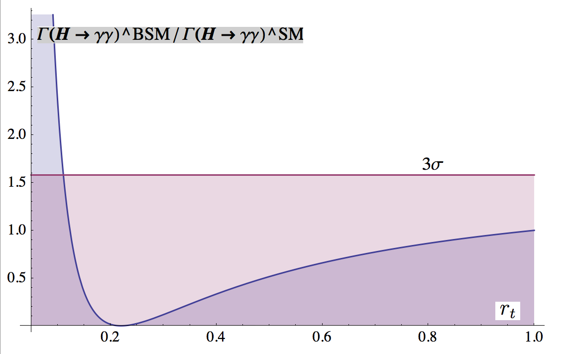
Figure 1: $\Gamma(H\rightarrow\gamma\gamma)$ for BSM/SM

The ratio of $\Gamma(H\rightarrow\gamma\gamma)$ for the BSM vs the SM as a function of $r_{t}$. The SM is on the curve at the point (1,1).

The combination of the above results suggests that some MSSM, PQ and Class II models are disfavored.

The next to leading order (NLO) percentage corrections to the decay width $\Gamma(H\rightarrow\gamma\gamma)$ has been calculated Passarino:2007fp where it is found that the electroweak and QCD correction are both about $2\%$ but of opposite signs, so they nearly cancel leading to a total correction of less than one percent compared with the leading order calculation.

Additional particles can alter the decay widths, as can the variations of the Yukawa couplings from their SM values on which we have focused. If the BSM Yukawas $Y_{i}^{BSM}$ do deviate from the SM values $Y_{i}^{SM}$, one may suspect additional states although the range of possibilities is too wide-ranging to analyze succinctly here. Even if we have focused on $H\rightarrow\bar{b}b,\bar{\tau}\tau,\gamma\gamma$ other decays such as $H\rightarrow VV$ where $V$ are vector gauge bosons can also be useful to probe departure from the SM.

Although the preliminary LHC data on H decay is presently of limited accuracy, it is nevertheless exciting that it is already enough to dispose of some examples of BSM models.

With the upcoming second run of the LHC, anticipated to begin in 2015 at higher energy and luminosity, one can confidently expect a great improvement in the accuracy of the measurements for the H partial decay modes and hence a better and more detailed check of the constraint sum rule. This heralds a new chapter of particle phenomenology. Constructing viable theories beyond the standard model will become very tightly constrained which is obviously a good thing. There are models with extra Higgs doublets that do not acquire VEVs, like inert Higgs models, that can avoid the sum rule constraint.

To conclude, we have found a sum rule that applies to BSMs that have more than one Higgs doublet with VEVs and Yukawa coupling to light fermions. The sum rule constrains all models of this type including but not limited to a large class of flavor symmetry models, 2HDMs, SUSY models including MSSM.

Acknowledgment: The work of TWK was supported by DoE grant# DE-SC0011981.

References

- (1) G. Aad et al. (ATLAS), Phys. Lett. B 716, 1 (2012) arXv:1207.7214 [hep-ex]; S. Chatrchyan et al. (CMS), Phys. Lett. B 716, 30 (2012) arXiv:1207.7235 [hep-ex];
- (2) S. Chatrchyan et al. (CMS), Phys. Rev. Lett. 110, 081803 (2013) arXiv:1212.6639 [hep-ex]; ATLAS Collaboration, ATLAS-CONF-2013-013; CMS Collaboration, CMS PAS HIG-13-002.
- (3) ATLAS Collaboration, ATLAS-CONF-2013-031; CMS Collaboration, CMS PAS HIG-13-003; ATLAS Collaboration, ATLAS-CONF-2013-029 and ATLAS-CONF-2013-040.
- (4) P. W. Higgs, Phys. Lett. 12, 132 (1964).
- (5) F. Englert and R. Brout, Phys. Rev. Lett. 13, 321 (1964).
- (6) G. S. Guralnik, C. R. Hagen and T. W. B. Kibble, Phys. Rev. Lett. 13, 585 (1964).
- (7) For a recent review of Higgs physics see M. Carena, C. Grojean, M. Kado and V. Sharma, in the 2013 partial update for the 2014 edition of J. Beringer et al. (Particle Data Group), Phys. Rev. D 86, 010001 (2012), [http://pdg.lbl.gov/2013/reviews/rpp2013-rev-higgs-boson.pdf].
- (8) G. Aad et al. (ATLAS), Phys. Lett. B 726, 88 (2013) arXiv:1307.1427 [hep-ex].
- (9) S. Chatrchyan et al. (CMS), Phys. Rev. D 89, 092007 (2014) arXiv:1312.5353 [hep-ex].
- (10) ATLAS Collaboration, ATLAS-CONF-2013-034; CMS Collaboration, CMS PAS HIG-13-005.
- (11) G. Altarelli and F. Feruglio, Rev. Mod. Phys. 82, 2701 (2010) arXiv:1002.0211 [hep-ph].
- (12) H. Ishimori, T. Kobayashi, H. Ohki, Y. Shimizu, H. Okada and M. Tanimoto, Prog. Theor. Phys. Suppl. 183, 1 (2010) arXiv:1003.3552 [hep-th].
- (13) P. H. Frampton and T. W. Kephart, Int. J. Mod. Phys. A 10, 4689 (1995) hep-ph/9409330.
- (14) N.G. Deshpande, E. Ma, Phys. Rev. D 18, 2574 (1978); E. Ma, Phys. Rev. D 73, 077301 (2006). hep-ph/0601225
- (15) A. Arhrib, R. Benbrik and T. -C. Yuan, Eur. Phys. J. C 74, 2892 (2014) arXiv:1401.6698 [hep-ph].
- (16) S. Chatrchyan et al. (CMS), JHEP 1405, 104 (2014) arXiv:1401.5041 [hep-ex].
- (17) (for ) ATLAS NOTE, ATLAS-CONF-2013-108, ATLAS Collab., November 28, 2013
- (18) M. T. Grippo et al. (CMS), Nuovo Cim. C 037, 293 (2014).
- (19) (for ) ATLAS NOTE, ATL-PHYS-PUB-2014-011, ATLAS Collab., July 4, 2014
- (20) G. C. Branco, P. M. Ferreira, L. Lavoura, M. N. Rebelo, M. Sher and J. P. Silva, Phys. Rept. 516, 1 (2012) arXiv:1106.0034 [hep-ph].
- (21) P. M. Ferreira, R. Santos, H. E. Haber and J. P. Silva, Phys. Rev. D 87 5, 055009 (2013) arXiv:1211.3131 [hep-ph].
- (22) G. Belanger, B. Dumont, U. Ellwanger, J. F. Gunion and S. Kraml, Phys. Rev. D 88, 075008 (2013) arXiv:1306.2941 [hep-ph].
- (23) B. Dumont, J. F. Gunion and S. Kraml, Phys. Rev. D 89, 055018 (2014) arXiv:1312.7027 [hep-ph].
- (24) J. R. Ellis, M. K. Gaillard and D. V. Nanopoulos, Nucl. Phys. B 106, 292 (1976).
- (25) B. L. Ioffe and V. A. Khoze, Sov. J. Part. Nucl. 9, 50 (1978) [Fiz. Elem. Chast. Atom. Yadra 9, 118 (1978)].
- (26) M. A. Shifman, A. I. Vainshtein, M. B. Voloshin and V. I. Zakharov, Sov. J. Nucl. Phys. 30, 711 (1979) [Yad. Fiz. 30, 1368 (1979)].
- (27) W. J. Marciano, C. Zhang and S. Willenbrock, Phys. Rev. D 85, 013002 (2012) arXiv:1109.5304 [hep-ph].
- (28) M. Shifman, A. Vainshtein, M. B. Voloshin and V. Zakharov, Phys. Rev. D 85, 013015 (2012) arXiv:1109.1785 [hep-ph].
- (29) R. Gastmans, S. L. Wu and T. T. Wu, arXiv:1108.5322 [hep-ph].
- (30) R. Gastmans, S. L. Wu and T. T. Wu, arXiv:1108.5872 [hep-ph].
- (31) G. Passarino, C. Sturm and S. Uccirati, Phys. Lett. B 655, 298 (2007) arXiv:0707.1401 [hep-ph].