Beyond KernelBoost

Abstract

In this Technical Report we propose a set of improvements with respect to the KernelBoost classifier presented in [3]. We start with a scheme inspired by Auto-Context, but that is suitable in situations where the lack of large training sets poses a potential problem of overfitting. The aim is to capture the interactions between neighboring image pixels to better regularize the boundaries of segmented regions. As in Auto-Context [32] the segmentation process is iterative and, at each iteration, the segmentation results for the previous iterations are taken into account in conjunction with the image itself. However, unlike in [32], we organize our recursion so that the classifiers can progressively focus on difficult-to-classify locations. This lets us exploit the power of the decision-tree paradigm while avoiding over-fitting.

In the context of this architecture, KernelBoost represents a powerful building block due to its ability to learn on the score maps coming from previous iterations. We first introduce two important mechanisms to empower the KernelBoost classifier, namely pooling and the clustering of positive samples based on the appearance of the corresponding ground-truth. These operations significantly contribute to increase the effectiveness of the system on biomedical images, where texture plays a major role in the recognition of the different image components. We then present some other techniques that can be easily integrated in the KernelBoost framework to further improve the accuracy of the final segmentation.

We show extensive results on different medical image datasets, including some multi-label tasks, on which our method is shown to outperform state-of-the-art approaches. The resulting segmentations display high accuracy, neat contours, and reduced noise.

roberto.rigamonti@epfl.ch http://cvlab.epfl.ch/ rigamont vincent.lepetit@epfl.ch http://cvlab.epfl.ch/ lepetit pascal.fua@epfl.ch http://cvlab.epfl.ch/ fua

School of Computer and Communication Sciences
Swiss Federal Institute of Technology, Lausanne (EPFL)

EPFL-REPORT-200378

July 22, 2014

1 Introduction

Many recent papers [32, 19, 17, 10] have shown the importance of using context when segmenting biomedical images. It helps avoid large segmentation errors without having to rely on ad hoc regularization priors [24, 15], which are commonly used but can only improve results to a limited extent. Using context in this manner can therefore be understood as learning to capture more complex interactions to better regularize the segmented regions.

Original image		Ground-truth
Random Forests		Improved KernelBoost
Auto-Context [32]		Our approach

Figure 1: Segmentation example for a test image from the Jurkat dataset [18] (the area highlighted in orange is ignored during training/testing, as it includes cells that do not appear in the ground truth). The thresholds were selected to give, for each method, the highest accuracy. Note that our approach finds accurate boundaries between the different regions, and that it avoids the errors made by the other methods especially in the light gray region. Red overlays in the segmentations are used to mark the mistakes. Best viewed in color.

(a)                               (b)                                           (c)

Figure 2: (a) Schematic representation of the Auto-Context approach [32]. At each iteration, the segmentation results from the previous iterations are taken into account in addition to the input image. (b) Ideal structure of our system, which we have dubbed Expanded Trees. The output of the first segmentation (Sc) is split between positive and negative samples, and two separate classifiers are trained. The procedure is iterated for the desired number of levels, and finally a classifier collects the different output to produce the final segmentation. Since we use powerful classifiers, many training samples are required, otherwise we would quickly run out of samples and therefore overfit after few iterations. Also, the number of classifiers to train – and therefore the computational costs – grows exponentially with the depth of the structure. (c) The approach we propose. We “knot” some branches together, and the classifiers in charge of a specific class at each level are now the same. This avoids overfitting, as the classifiers are trained with larger training sets, while retaining most of the classification power of the tree structure and keeping the computational effort limited. Again, the output of all the intermediate steps is fed to a classifier that produces the final segmentation.

In this paper, we go one step further by showing that we can use context not only to avoid segmentation errors but also to accurately find region boundaries. This is challenging for several reasons. First, in most kinds of images, classifiers trained to differentiate locations belonging to one kind of region from those belonging to another may struggle near boundaries. This is because locations on both sides of the boundaries can be hard to distinguish, especially when using feature vectors computed using filters having a substantial spatial extent. Second, in biomedical images in general and particularly in those at the scale of living cells, boundaries can have arbitrarily complex shapes.

To overcome these difficulties we propose an approach that is inspired by the popular Auto-Context algorithm [32] but, unlike it, progressively focuses more and more on difficult-to-classify samples.

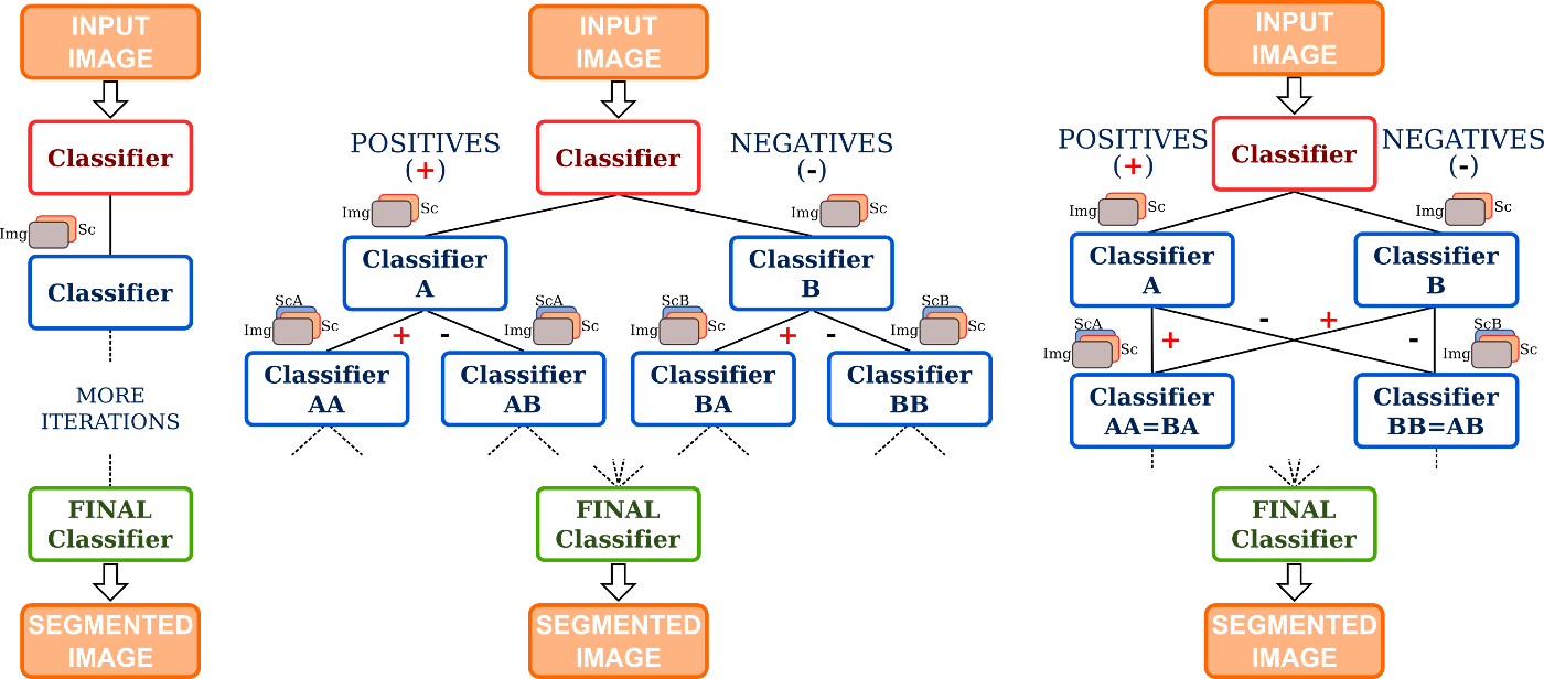
More specifically, for foreground/background segmentation purposes, Auto-Context trains a chain of classifiers as depicted by Fig. 2(a): The input to the first classifier is simply the image data but the next classifiers also have access to the segmentation results produced by previous stages. To achieve our goal of focusing on difficult-to-classify samples, we could instead leverage the powerful decision tree strategy [5]. This would mean recursively splitting the pixels into those that are classified as foreground and background and train a new classifier for each subset, as depicted by Fig. 2(b). Unfortunately, unless the training set is sufficiently large, that would be suboptimal because each subsequent classifier would have to be trained on an ever smaller fraction of it, to the point where the training would become ineffective. This is particularly true in the biomedical field, where often the amount of training data is limited because it is cumbersome to label. Also, this would require the training of an exponentially growing number of classifier, and therefore a considerable computational effort. We will refer to this approach in the following as Expanded Trees.

As shown in Fig. 2(c), our solution is to train only two classifiers at each stage. The first operates on the samples that are classified as potential foreground ones by either classifiers at the previous stage, and the second one on samples classified as potential negatives. In this way, the number of training examples used to train the classifiers can be kept roughly constant at all stages, which avoids overfitting. Since we “knot” the two branches of the tree, we have dubbed this approach Knotted Trees. To focus on the difficult-to-classify examples, we use permissive bounds to decide if a sample is potentially foreground or background. For example, a sample classified as negative but with a low confidence score is a difficult-to-classify sample, and it is sent to the two classifiers at the next stage. In this way, both classifiers will have access to these important samples. A final classifier collects the partial results from the different branches and outputs the final segmentation.

In the evaluation of the schemes we presented, we use in each node a KernelBoost classifier [3]. However, other classifiers can be used as long as they are powerful enough, at least in the earlier stages.

Our approach naturally extends to multi-label segmentation problems. We simply train our approach for each label in a 1-versus-1 scheme, where separate binary problem are set up for each pair of classes. Again, a final classifier collects the partial results from the different branches and outputs the final segmentation.

We use four different datasets to demonstrate that our approach outperforms both Auto-Context [32] and a recent CRF-based method [15], and to assess the strengths and weaknesses of the methods we propose.

2 Related Work

Image segmentation algorithms typically rely on local image cues combined with spatial constraints. For example, Markov Random Fields (MRFs) use unary terms that depend on image features together with pairwise potentials that enforce simple smoothness priors [12, 21]. With Conditional Random Fields (CRFs), the smoothness terms can also be made dependent on the image cues [30, 22]. This can exploit the fact that boundaries between image regions have specific image appearance, and significantly improves the quality of the resulting segmentation.

However it is not entirely clear that simple spatial features truly make a difference when powerful image features are used, and several authors report good results even without spatial constraints [23, 33, 26, 14]. Higher orders terms [9] or hierarchical approaches [11] have therefore been introduced to capture more global constraints. Unfortunately, optimizing the parameters of such complex models in CRFs quickly becomes intractable. [20] shows that decision trees can be used in Decision Tree Fields to model both the unary and the pairwise terms. This makes the parameter estimation problem much more tractable. [15] relies on subgradient descent to efficiently learn CRF models for segmentation using a working set of constraints in a Structured SVM formulation. This method obtains state-of-the-art results on medical data, and we compare against it in the Experimental Results section.

However despite the widespread interest in them, CRFs are still computationally expensive at run-time. A more efficient approach to enforcing spatial constraints was introduced in [32] under the name of Auto-Context. In Auto-Context, a first segmentation is obtained by simple pixel-wise segmentation, followed by a second segmentation obtained by combining image features with “context features”. They are similar to image features but are computed on the output of the first iteration. This process can be iterated until convergence. This scheme was inspired by [13]. A similar approach was also developed in [26] together with a CRF model. Entangled Forests [17] use similar features in the nodes of Random Forests, applied to the output of previous nodes. Geodesic Forests [10] extend these features to depend on geodesic distances between pairs of locations to exploit long-distance correlations. However using the geodesic distances assumes that strong image gradients are highly correlated with boundaries between regions, which is often not true in medical images, as shown in Figs. 1, 3, and 6.

We also use features computed from previous segmentations. However we show how to leverage this general approach to significantly improve the quality of the final segmentation, by focusing on the difficult-to-classify locations.

The idea of splitting samples according to the estimated probabilities was already proposed in [31], but they adopt a traditional binary tree structure, they do not pass the estimated probabilities down the tree to enrich the input features – therefore they lack context information –, they do not learn features on the newly estimated probabilities, and they do not have a final classification stage.

3 Our Approach

In this section we describe our approach. It relies on a statistical segmentation method that can take as input the original image and the results of the previous segmentation steps. In practice we use the KernelBoost method [3], which we improved for this work. We therefore describe it in Section 4 for completeness, along with our modifications.

3.1 Knotting Branches for Segmentation

In our approach, as illustrated in Fig. 2(c), we first segment the input image using a classifier that predicts for each image location to which class the location belongs, together with a confidence measure about this prediction.

In general this first segmentation has margins for improvement, and we perform subsequent segmentations that rely not only on the original image but also on the output of previous steps.

This is similar to what Auto-Context does, but differs in a critical way: we separate image locations into a “positive set” made of the ones classified as positives, and a “negative set” made of the ones classified as negatives. Each set is then processed independently by a new classifier. We iterate this process until convergence on the training set. The output of the different classifiers are then fed to a final classifier to produce the final segmentation.

More formally, let $\mathcal{T}=\{({\bf X}_{i},{\bf Y}_{i})\}_{i}$ be a set of training images ${\bf X}_{i}$ together with the corresponding ground truth labels ${\bf Y}_{i}$. We write

$${\bf Y}_{i}(u,v)=\left\{\begin{array}[]{cc}+1&\text{ if }(u,v)\text{ in }{\bf X}_{i}\text{ belongs to foreground,}\\ -1&\text{ otherwise.}\\ \end{array}\right.$$ (1)

We train a first classifier

$$\varphi^{0}=\operatorname*{\arg\!\min}_{\varphi}\sum_{i}\sum_{(u,v)}L\big{(}{\bf Y}_{i}(u,v),\varphi({\bf X}_{i})(u,v)\big{)}\>,$$ (2)

where $L$ is a loss function.

$\varphi^{0}({\bf X})$ can be seen as a confidence map: $|\varphi^{0}({\bf X})(u,v)|$ is a confidence measure for location $(u,v)$ in ${\bf X}$. However, to avoid locations with large absolute values bias the further steps, we use instead a version normalized to lie in the $[-1,+1]$ by considering

$$\overline{\varphi}^{0}({\bf X})=2p\left({\bf Y}_{i}=1\left|\right.{\bf X}_{i}\right)-1,$$ (3)

where $p\left({\bf Y}_{i}=1\left|\right.{\bf X}_{i}\right)$ is the probability of a pixel of being in the positive class. We use

$$p\left({\bf Y}_{i}=1\left|\right.{\bf X}_{i}\right)=\frac{1}{1+\exp(-2\varphi^{0}({\bf X}))}$$ (4)

as in [8].

We then define the positive $P_{i}^{0}$ and negative $N_{i}^{0}$ sets for each training image ${\bf X}_{i}$ as

$$\begin{array}[]{ll}P_{i}^{0}&=\left\{(u,v)\>|\>\overline{\varphi}^{0}({\bf X}_{i})(u,v)>-\varepsilon\right\}\>,\text{ and}\\ N_{i}^{0}&=\left\{(u,v)\>|\>\overline{\varphi}^{0}({\bf X}_{i})(u,v)<+\varepsilon\right\}\>.\\ \end{array}$$ (5)

Because we use $\varepsilon>0$, the positive sets $\{P_{i}^{0}\}_{i}$ contain locations that are classified by $\overline{\varphi}^{0}$ as positive but also locations classified as negative but with low confidence. In practice, we use $\varepsilon=\frac{1}{2}$. Similarly, the negative sets $\{N_{i}^{0}\}_{i}$ contain locations classified as positive with low confidence. Both the positive and negative sets therefore contain all the difficult-to-classify samples, which will be treated by two new classifiers $\varphi_{P}^{1}$ and $\varphi_{N}^{1}$. The first is taken to be

$$\begin{array}[]{ll}\varphi_{P}^{1}=&\operatorname*{\arg\!\min}\limits_{\varphi}\sum\limits_{i}\sum\limits_{(u,v)\in P_{i}^{0}}L\big{(}{\bf Y}_{i}(u,v),\varphi({\bf X}_{i}^{1})(u,v)\big{)}\>,\\ \end{array}$$ (6)

where ${\bf X}_{i}^{1}=\big{(}{\bf X}_{i},\overline{\varphi}^{0}({\bf X}_{i})\big{)}$. $\varphi_{P}^{1}$ is therefore trained on the locations in the positive sets only, and has access to the normalized confidence maps $\overline{\varphi}^{0}({\bf X}_{i})$ in addition to the training images. Its task is thus simpler than that of the first classifier. The $\varphi_{N}^{1}$ classifier is defined in a similar way.

New positive and negative sets, respectively noted $P_{i}^{1}$ and $N_{i}^{1}$, are computed as before from the output of the two classifiers $\varphi_{P}^{1}$ and $\varphi_{N}^{1}$. Next, we train a second pair of classifiers $\varphi_{P}^{2}$ and $\varphi_{N}^{2}$. The $\varphi_{P}^{2}$ classifier is taken as:

$$\begin{array}[]{ll}\varphi_{P}^{2}=&\operatorname*{\arg\!\min}\limits_{\varphi}\sum\limits_{i}\sum\limits_{(u,v)\in P_{i}^{1}}L\big{(}{\bf Y}_{i}(u,v),\varphi({\bf X}_{i}^{2,P})(u,v)\big{)}\>,\\ \end{array}$$ (7)

where ${\bf X}_{i}^{2,P}$ is made of image ${\bf X}_{i}$, and all the corresponding confidence maps computed up to this point: ${\bf X}_{i}^{2,P}=\big{(}{\bf X}_{i},\overline{\varphi}^{0}({\bf X}_{i}),\overline{\varphi}_{P}^{1}({\bf X}_{i}^{1})\big{)}$. Similarly,

$$\begin{array}[]{ll}\varphi_{N}^{2}=&\operatorname*{\arg\!\min}\limits_{\varphi}\sum\limits_{i}\sum\limits_{(u,v)\in N_{i}^{1}}L\big{(}{\bf Y}_{i}(u,v),\varphi({\bf X}_{i}^{2,N})(u,v)\big{)}\>,\\ \end{array}$$ (8)

This process is iterated as long as the numbers of misclassified samples in both branches of our “tree” remain above a threshold.

Finally we train a Randomized Forest to predict the locations labels based on all the available data, including the input image, feeding the classifier with a feature descriptor

$$\Delta=\Big{\{}\Big{(}\big{(}{\bf X}_{i},\overline{\varphi}^{0}({\bf X}_{i}),\overline{\varphi}_{P}^{1}({\bf X}_{i}^{1}),\overline{\varphi}_{N}^{1}({\bf X}_{i}^{1}),\cdots\big{)},{\bf Y}_{i}\Big{)}\Big{\}}_{i}.$$ (9)

To incorporate additional information about a pixel’s neighborhood, we also consider the values located on the corners and on the middle of the side of two nested squares centred on the point, with side of 5 and 10 pixels respectively, in a stylized snowflake configuration.

In the case of a multi-label segmentation problem, we proceed as described above for each label in a 1-versus-all scheme. Again, a final Randomized Forest is trained to predict the label based on all the intermediate data created for all the labels.

At run-time, we simply have to apply to the input image ${\bf X}$ the successive classifiers $\varphi^{0}$, $\varphi_{P}^{0}$, $\varphi_{N}^{1}$, $\cdots$ to compute the normalized confidence maps, which are then fed to the final Randomized Forest to obtain a final confidence map.

3.2 Expanded Trees

In the case of the ideal structure of Fig. 2(b), we proceed as explained above for what concerns the splitting criteria, but instead of sending samples to the parallel branch when they meet the criteria to switch branch, we simply continue the splitting process. When the number of samples in a node falls below a critical threshold, we stop the growing of that branch.

4 KernelBoost, Improved KernelBoost, and extensions

KernelBoost (KB) is a statistical method that segments an image by classifying each pixel independently into two classes. It has the key advantage of not requiring to hand-design the kernels it operates with, and that of having very few, easily tunable parameters.

The training data is a set of training samples $\{({\bf x}_{i},y_{i})\}_{i=1...N}$, where ${\bf x}_{i}\in{\mathbb{R}}^{n}$ is an image patch and $y_{i}\in\{-1,1\}$ its corresponding label. From this set, KernelBoost first generates a bank of discriminative kernels, and then builds a binary GradientBoost classifier, with weak learners of the form of regression trees. Each node of these trees contains a test selected from the kernel bank. At run-time, the selected kernels ${\bf k}_{j}$ can simply be used as convolutional filters applied to the image to segment, which makes the approach efficient.

4.1 Pooling and training sample clustering

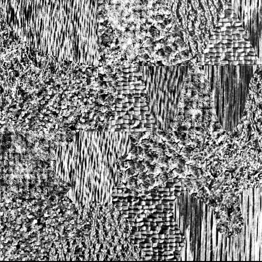
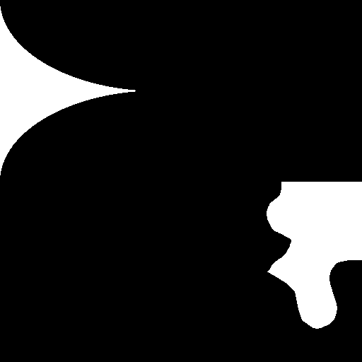
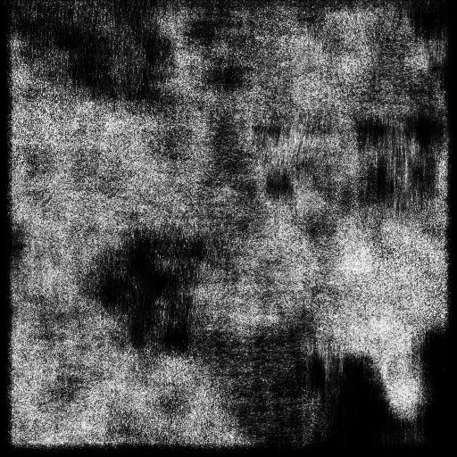
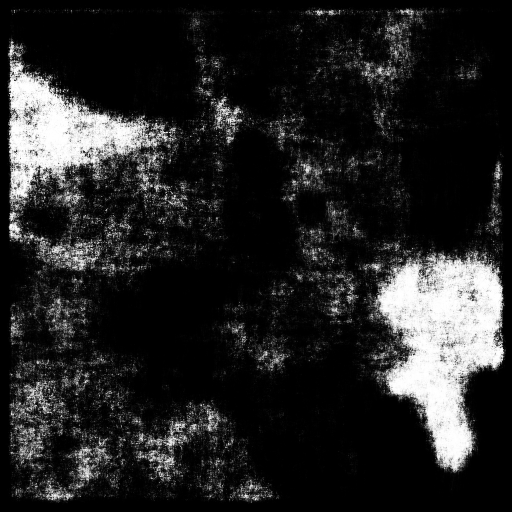
While obtaining excellent performances in the delineation of curvilinear structures [3], the original KernelBoost method lacks a mechanism for dealing with more complex patterns, such as the ones that typically appear in medical images. To highlight this deficiency, we applied the original KernelBoost to a texture segmentation problem. As shown in Fig. 3(c), the quality of the segmentation is quite poor.

(a)		(b)
(c)		(d)

Figure 3: Texture experiment. The segmented image is a mosaic of Brodatz images, created at USC-SIPI for research on texture segmentation. The dataset is available at the address http://sipi.usc.edu/database/?volume=textures. (a) Original test pattern. (b) Ground-truth for the selected material. (c) Segmentation obtained by the KernelBoost algorithm [3]. (d) Segmentation obtained by the KernelBoost algorithm coupled with the POSNEG/MAX-pooling scheme.

This is because, for texture recognition problems, the filter responses should be made robust to slight shifts in the images. We therefore introduce a pooling mechanism [4] over the filter responses. We evaluated several possible mechanisms, and we empirically noticed that keeping the maximum value of the responses of the POSNEG operator [25] over a region performed best.

The POSNEG operator transforms the result of a convolution $C$ into two images, one made of the positive values of $C$, the other one made of the opposite of the negative values of $C$. The optimization over each node finds which filter and which of these two images should be used for best performances.

Moreover, the kernels learned by the original KernelBoost filters are not always optimal. This is because they are learned in a discriminative fashion in the attempt to distinguish all the positive samples from the negative ones. However, this leads to suboptimal performances because positive samples can be very different from each other, for example in presence of texture.

We therefore cluster the positive samples based on their appearances, and each kernel is generated by classifying the positive samples of one cluster randomly chosen against all the negative samples. We empirically observed that this second modification also improves the results compared to the original KernelBoost.

However, even with these improvements, KernelBoost can make significant mistakes if not incorporated in the framework we propose, as shown in Fig. 1. In the following we will refer to KernelBoost, when both pooling and clustering are used, as Improved KernelBoost (IKB for short).

4.2 Superpixel pooling and superpixel features

Superpixels [7] emerged as an efficient way of dealing with large images and image stacks, while at the same time improving the performances by averaging the results of pixel-based approaches over small, homogeneous image regions. The idea behind them is to group meaningful regions and to use them as a substitute of the regular grid structures imposed by pixels [1]. The same pixel-based regular grid is used by traditional pooling operators available in literature, we have therefore considered replacing it with a structure based on superpixels. However, given the homogeneity of the pixels captured inside each superpixel, pooling the feature values inside each superpixel would be of little use. Indeed, the main goal of the pooling step is to introduce robustness against small distortions, translations and rotations, and this requires the pooling scheme to be independent from the underlying data.

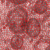
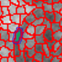
The idea of analyzing filter responses over structures whose shapes are not imposed by rigid rules, but by the image itself, is nonetheless appealing. We have therefore considered not the superpixels extracted from the images, but the regions which can be computed from them by erosion and dilation by a given amount of pixels. If we consider, for instance, the superpixel segmentation of Fig. 4(a), we can observe that it is able to group interesting regions, such as the membranes of the mitochondria. While pooling directly on them would simply average very similar filter responses on an homogeneous region, if we consider smaller and larger regions we can hope that, for instance, the classifier gets fed with the border of each membrane, easing its recognition. As an example, this can happen by considering the two regions, outlined in green and blue respectively, of Fig. 4(b). We have dubbed this approach superpixel pooling.

(a)	(b)

Figure 4: Analysis of the regions identified by SLIC superpixels [1] on a fragment of a medical image. (a) SLIC superpixels extracted by the code provided by [1]. Notice that they accurately distinguish different regions, such as the membranes of the mitochondria. (a) Example extended/shrinked regions — in blue and green respectively — where pooling can be performed to extract meaningful information about the mitochondrion’s membrane.

In the KernelBoost context we can go even further and perform operations over different regions computed from the individual superpixels. The classifier present in each weak learner will be fed with a set of features resulting from potentially nonlinear operations over multiple regions — for instance the difference of the absolute values of the negative parts of the two regions in Fig. 4(b) — and will then be able to select the most discriminative combinations for a given training set.

Among the different approaches available in literature, SLIC superpixels [1] emerged for their simplicity and their capability to adhere to image boundaries. We have therefore based our proposal on the superpixels extracted by this approach.

4.3 External features

KernelBoost is particularly well suited to exploit the power of external hand-crafted or learned features. It can indeed load them as additional channels, and perform filter learning on them, thus empowering them by building a two-level architecture. A particularly interesting example of features is constituted by Ilastik features [28]. They are constituted by multiple hand-crafted features — such as Gaussians, Structure Tensor, …— computed with different parameter settings, for instance different Gaussian smoothing. They are used in many state-of-the-art segmentation tools used by practitioners.

The features that can be used are usually dataset-dependent. For instance, in one dataset where the task is the segmentation of mitochondria, we have included as an additional channel the mitochondria membranes obtained by the algorithm of [27], and this proved to significantly improve the final performance, as shown in Section 5.

4.4 Multiple scales

When dealing with medical images, the structures of interest commonly appear at very different scales or occupy relevant portions of the images. In typical EM images of mitochondria, for example, a single mitochondrion might be several hundreds pixels in length. For this reason, learning filters from data at full image scale might lead to a set of filters which are able to capture only small fractions of the objects, engendering errors in a pixel-level segmentation.

The KernelBoost approach can be easily extended to deal with multiple scales, given its ability to operate on separate input channels. We just have to incorporate the notion of scale in the sampling scheme, to ensure that the same sample is collected over the different scales considered. The filter learning process is then performed independently for each individual channel at the proper scale, and the regression tree learning scheme will then be in charge of selecting which filter and which scale are more discriminative.

4.5 Fake-3D

EM imagery often produces complete, anisotropic image stacks. Full 3D information can be very useful in discriminating the different components of the scene, but it is usually computationally expensive and memory intensive to deal with. Moreover, the anisotropicity of the data might result in degenerate filters and therefore poor performance. For these reasons, while KernelBoost could in principle operate on N-D data — experiments with 3D image stacks are presented in [3] — we have chosen to operate on 2D data but incorporating data from multiple neighboring slices. In particular, the whole segmentation scheme operates on individual slices until it reaches the final classifier stage. At that point the classifier is fed not only with the features extracted on the considered slice, but also with the features extracted on a slice $D$ steps before and on a slice $D$ steps after it. Padding is performed to deal with stack’s boundaries. We have considered in our experiments $D=3$, but its exact value has to be tuned according to the size of the structures of interest and the inter-slice distance.

4.6 Z-cut

Biomedical image stacks usually contain components with no predominant orientation. The choice of the axes is therefore arbitary. When enough slices are available, it might be interesting to consider not only the images in the traditional X-Y plane, but also in the X-Z and Y-Z ones. This is particularly useful in the context of an architecture such as those presented in the previous chapter, where different levels of recursion can focus on different image planes. Indeed, if the anisotropicity is not too elevated, filters can impose a regularity on the structures found in these planes, giving a final 3D result which is smoother and less noisy.

5 Experimental Results

To validate our approach we performed extensive experiments on four very different medical image datasets.

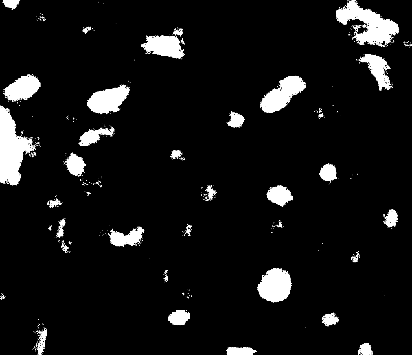
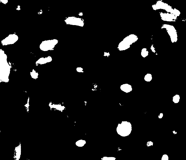
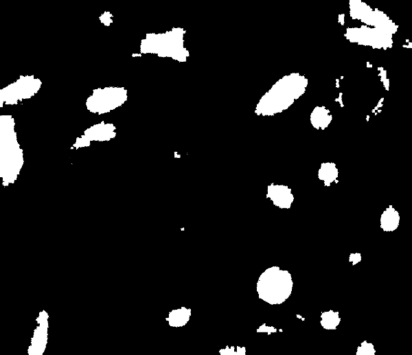
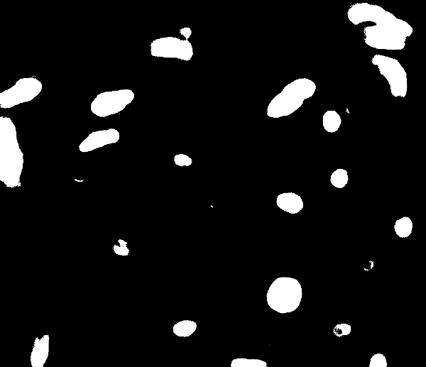
5.1 The Human T-Cell Line Jurkat Dataset [18]

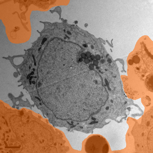
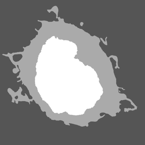
The first dataset we consider is composed by Transmission Electron Microscopy (TEM) images of the human T-cell line Jurkat [18]. We randomly selected 10 training images and 4 test images, each with size $1024\times 1024$ pixels. We then created a set of masks to ignore, both in training and in testing, the components that are not considered in the available ground-truth images. The particularity of this dataset is that it contains three different classes, for the background, the cytoplasm, and the nuclei. A sample training image, along with the corresponding ground-truth, is depicted by Fig. 1. The goal of the final user of this data is to estimate, with the higher accuracy possible, the areas of the different components of the cells, in order to use these values to tune numerical models of the response of illnesses to different treatments.

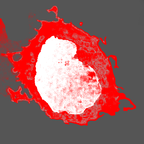
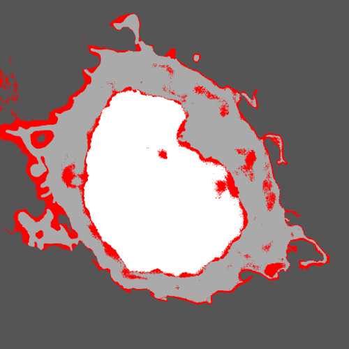
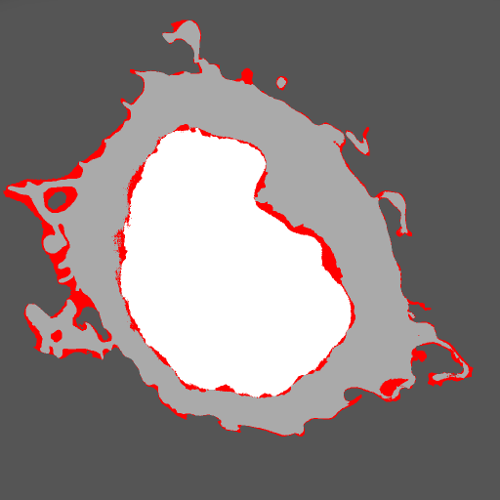
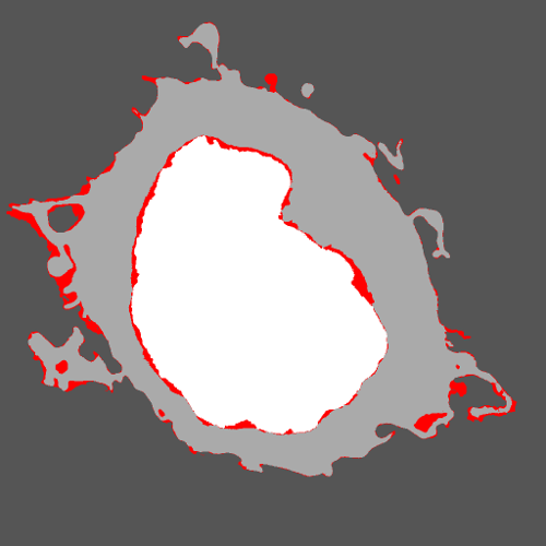
The main challenge of this dataset is the fact that the cytoplasm and the cell’s nucleus look very similar. The results obtained by the different approaches are given in Table 1. Our proposal significantly outperforms the other methods, including that of [16]. Visual inspection of our approach, as seen in Fig. 1, shows that not only the accuracy score is higher, but also the contours are significantly better delineated and macroscopic mistakes get fixed.

Table 1: Results for the Jurkat dataset [18]. The segmentation accuracy is computed as the fraction of pixels whose label match the ground-truth data. See Section 5.1 for more details.

Method	Accuracy
Random Forests	0.753
Lucchi et al. [16]	0.836
Improved KernelBoost	0.929
Auto-Context [32] (on Improved KernelBoost)	0.956
our approach (on Improved KernelBoost), no norm.	0.941
our approach (on Improved KernelBoost)	0.973

Table 1 also shows that normalization of the classifiers’ output as expressed by Eq. (3) is an important step, as the results without it are not significantly better than the ones obtained with the original Improved KernelBoost method on this dataset.

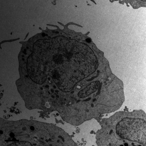
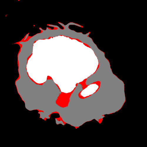
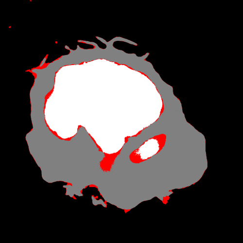
Finally, we have applied the Auto-Context approach [32] on the output of the Improved KernelBoost method. While Auto-Context improves the segmentation results for this dataset, the improvement is smaller than that achieved by our strategy. Fig. 5 shows how errors are distributed for different approaches on a test image. Note also that what we have labeled Auto-Context is an improved version of the algorithm of [32], since filters are learned at each stage on the newly added score images, and the final set of score maps is used to feed a Random Forest classifier instead of simply relying on the last score map. In our tests with methods that do not learn filters on the feature maps, for instance [2], the improvements linked with the use of Auto-Context are negligible.

Original image	Auto-Context [32]	Our approach

Figure 5: Segmentation errors for a test image from the Jurkat dataset [18]. The errors are highlighted in red in the images. Our approach significantly reduces the mistakes — the accuracy for our approach is 0.972, while it is 0.956 for Auto-Context. Best viewed in color.

To validate our results, we have randomly selected another set of 10 training and 6 testing images — denoted here as Jurkat-B dataset —, and we have reported the results obtained by the three methods of Fig. 2 in Table 2. As it can be seen, our approach performs better then Auto-Context — which is reasonable and confirms the results obtained in the other random split — but also the Expanded Trees, since the amount of training images is limited and therefore the system might suffer because of that.

Table 2: Results for the Jurkat-B dataset [18].

Method	Accuracy
KernelBoost	0.909
Auto-Context [32] (on KernelBoost)	0.922
Expanded Trees (on KernelBoost)	0.934
Knotted Trees (on KernelBoost)	0.948

5.2 NIH-3T3 Fibroblast Cells Dataset [6]

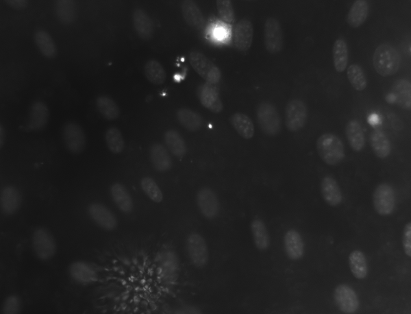
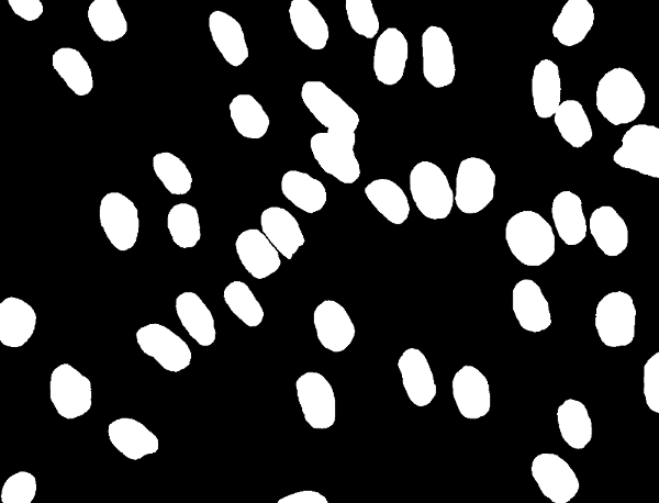
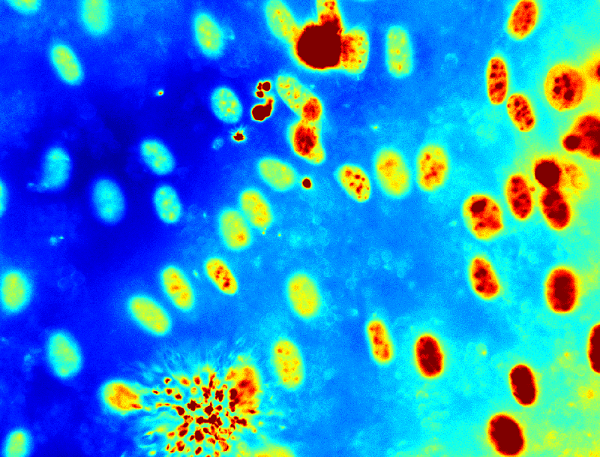
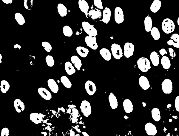
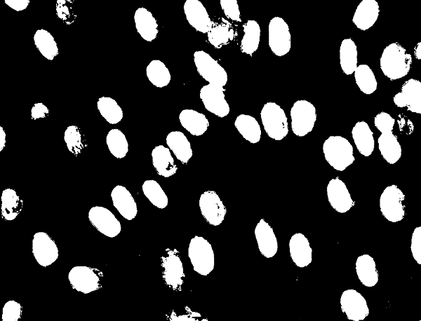
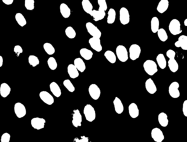
The second dataset we consider is constituted by 2D fluorescence microscopy images of Hoechst 33342-stained NIH-3T3 mouse embryonic fibroblast cells [6]. As it can be seen in the sample test image depicted by Fig. 6, the images often contain debris and the nuclei vary greatly in brightness, making their segmentation challenging. For these reasons, this dataset was chosen for one of the competitions in the ISBI2009 challenge. The training set is composed by 4 randomly chosen test images with size $1344\times 1024$ pixels, while the test set contains the remaining 45 images.

(a)		(b)
(c)		(d)
(e)		(f)

Figure 6: Segmentation results for a randomly-selected test image from the NIH-3T3 fibroblast cells dataset [6]. The thresholds used to obtain the segmentations from the score images are given by the values that maximize the VOC score for the given image. (a) Original test image. The poor contrast exhibited by the images is one of the characteristics that make this dataset difficult. (b) Ground-truth for the selected image. (c) Original test image, after being manually altered to improve the visual quality. Best viewed in colors. (d) Segmentation obtained with Improved KernelBoost. The VOC score is 0.7243. (e) Segmentation obtained by our approach except that the samples are split into two balanced sets instead of a positive and negative sets. The VOC score is 0.8024. (f) Segmentation obtained by our approach. The VOC score is 0.8160.

Table 3 shows that our approach, using our Improved KernelBoost for the $\varphi$ classifiers, significantly outperforms the state-of-the-art algorithm for this dataset [29], as well as the other methods we evaluated. Our approach improves on the starting point, given by Improved KernelBoost, which in turn is better than the original KernelBoost classifier. It is also better than Auto-Context, which does not bring a significative improvement over the starting point.

Table 3: Segmentation accuracy for the NIH-3T3 fibroblast cells dataset [6]. The results for the human expert were obtained by a second human expert on a subset of 5 images of the test set, and are given only to demonstrate the complexity of the task. See Section 5.2 for more details.

Method	VOC	RI	DI
Human expert [6]	-	0.93	-
Song et al. [29]	0.852	0.932	0.906
KernelBoost	0.817	0.921	0.899
Improved KernelBoost	0.833	0.929	0.909
Auto-Context (on Improved KernelBoost)	0.842	0.920	0.914
our approach (on Improved KernelBoost)	0.874	0.946	0.932
same, but with 50%-50% split	0.842	0.906	0.914

We also investigated the impact of splitting the samples in two balanced sets rather than splitting the samples classified as positives from the ones classified as negatives. As shown in the last row of Table 3, this gives results very similar to those of Auto-Context, demonstrating again the advantages of splitting the samples according to the scheme we propose.

5.3 3D Electron Microscopy Stacks [15]

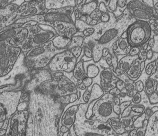
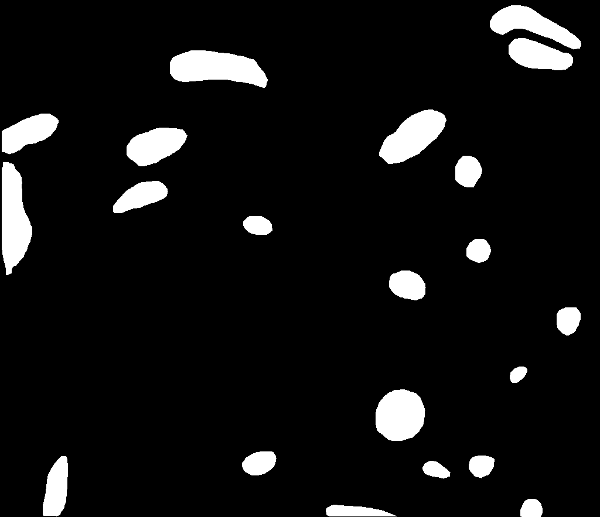
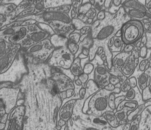
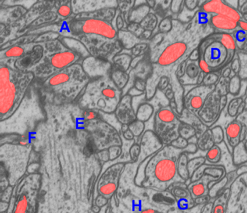
Our third dataset is composed by two 3D Electron Microscopy (EM) stacks of the CA1 hippocampus region of a rodent brain [15]. The training volume contains 165 slices with size $1024\times 653$ pixels, while the test volume has the same number of slices but with size $1024\times 883$ pixels. A sample slice, along with its corresponding ground-truth, is depicted by Fig. 7. The goal is to segment the mitochondria.

(a)		(b)
(c)		(d)
(e)		(f)

Figure 7: Segmentation results for a test image from the CA1 Hippocampus dataset [15]. The image has been randomly selected, but taken away from the stack’s borders to avoid penalizing the method of [15] which otherwise could not exploit neighboring slices to improve its result. The thresholds used to obtain the segmentations from the score images are given by the values that maximize the VOC score for the given image. (a) Original test image. (b) Ground-truth outlining the mitochondria in the selected image. (c) Segmentation obtained by KernelBoost. The VOC score on this image is 0.567. (d) Segmentation obtained by KernelBoost + pooling + clustering. The VOC score on this image is 0.632. (e) Segmentation obtained by the approach of [15]. The VOC score on this image is 0.679. (f) Segmentation obtained by our approach. The VOC score on this image is 0.719.

As Table 4 shows, we outperform the state-of-the-art algorithm [15], even though we operate on 2D slices only for simplicity, without enforcing any consistency between consecutive slices, while the approach of [15] relies on a 3D CRF.

Table 4: Results for the CA1 Hippocampus dataset [15]. The values have been computed by ignoring a 1-pixel width region around the mitochondria to account for imprecisions in the manual segmentations. See Section 5.3 for more details.

Method	VOC	F-measure
Lucchi et al. [15]	0.722	0.839
KernelBoost	0.625	0.769
KernelBoost + pooling only	0.649	0.787
Improved KernelBoost	0.711	0.831
our approach (on Improved KernelBoost)	0.776	0.874

From the table, it is also possible to appreciate the contribution given by the pooling and sample selection steps as explained in Section 4 with respect to the original KernelBoost method. A visual analysis of the segmentation mistakes is given in Fig. 8.

(a)		(b)

Figure 8: Analysis of the major segmentation mistakes made by our algorithm on a test image from the CA1 Hippocampus dataset [15]. (a) Original image. (b) Original image with the segmentation we have obtained overlayed. We have selected this image because the segmentation presents several mistakes, affecting significantly the final score. (A) The strong background difference in the mitochondrion makes our algorithm prematurely end the segmentation. (B) The two mitochondria are very close, and the texture between them mislead our algorithm. (C) Error in the ground-truth: the component identified by our algorithm is indeed a mitochondrion. (D) Two shadowed parts of the image are incorrectly identified as mitochondria, probably due to the borders on both sides (such structures are not present in the training data). (E,F) Minor mistakes due to shadows in the image. (G) Error in the ground-truth: a component is incorrectly identified as a mitochondrion, while it is not. (H) Dark element on the image’s border incorrectly identified as a mitochondrion. Best viewed in color.

Furthermore, we have randomly chosen a small subset of this dataset — 9 training and 6 test images — to perform an in-depth analysis of the performance of the different KernelBoost components listed in Section 4. The results are presented in Table 5.

Table 5: Comparison of the effectiveness of the different KernelBoost components on a subset of the CA1 Hippocampus dataset [15].

Method	VOC
KB	0.592
KB + pooling	0.638
KB + clustering	0.599
KB + pooling + clustering	0.638
KB + Ilastik features	0.667
KB + Ilastik features + pooling	0.673
KB + superpixel pooling	0.653
KB + superpixel pooling + superpixel features	0.660
KB + Ilastik features + superpixel pooling	0.683

In the case of this subset clustering does not seem to be that relevant. This might be due to the size of the dataset, as categorizing the positive samples might overly reduce the pool of samples used for the filter learning step. Pairing the input image channel with Ilastik features seems to be an interesting opportunity, as this allows to achieve very good performance. However, adding a pooling step on top of this does not increase significantly the performance. This can be explained by the fact that the smoothed images that are included in the Ilastik features can partially compensate for the lack of a pooling step. Superpixel pooling represents an effective strategy to improve the performance of the system, although computationally expensive. Adding on the top of it superpixel features does not significantly improve the final result. Finally, the pair superpixel pooling/Ilastik features performed best, achieving a VOC score that is almost 10% higher than the original KernelBoost score.

From the insights given by these experiments, we performed extensive tests on the architectures presented in Section 4. The results are given in Table 6.

Table 6: Comparison of the architectures of Section 4 on the CA1 Hippocampus dataset [15]. The base result is given by KernelBoost with Ilastik features, and all the subsequent processing starts from the score maps this method produces. Although very effective, we have skipped superpixel pooling because of its high computational costs.

Method	VOC
KernelBoost + Ilastik features	0.654
Auto-Context	0.701
Auto-Context + pooling (on image channel only)	0.704
Auto-Context + pooling (on all channels)	0.714
Auto-Context + pooling (on image channel only) + fake3D	0.735
Expanded Trees + pooling (on image channel only)	0.720
Expanded Trees + pooling (on image channel only) + fake3D	0.746
Knotted Trees + pooling (on image channel only)	0.717
Knotted Trees + pooling (on image channel only) + fake3D	0.743
Knotted Trees + pooling (on image channel only) + fake3D + Z-cut	0.762

The results show that pooling on all the channels — thus including the score images from the previous iterations — slightly improves the segmentation results. A more significative contribution comes, as expected, from the fake3D approach and the Z-cut. In this experiment the Expanded Trees performed 0.3% better than Knotted Trees — a negligible difference that shows that in presence of enough training samples the two architectures are equivalent, while the experiments on the Jurkat dataset show the superiority of Knotted Trees when few training samples are available.

5.4 2D Electron Microscopy Cell dataset

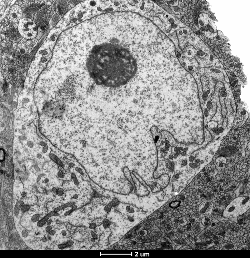
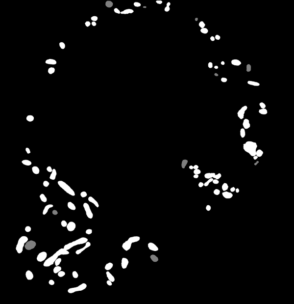
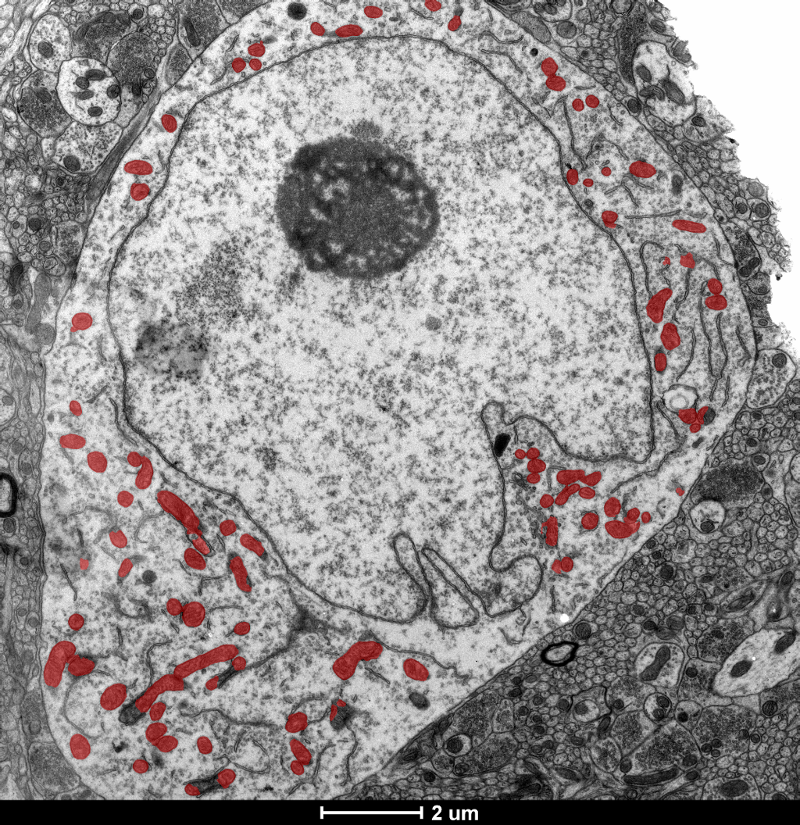
The last dataset is composed by 2D EM images of cells. The images are high-dimensional (4096 $\times$ 4224), and we randomly selected 8 images for training and 4 for testing. The goal is to segment the mitochondria inside the cell, when masks excluding the outside of the cell and the nuclei are provided. An example image is given in Fig. 9, along with the corresponding ground-truth. Without additional information some structures appearing in the images are not clearly categorizable by a human expert. We have therefore introduced a third class, depicted in gray in the ground-truth, to account for these elements. This makes the problem more complex, but allows the final user to individually select whether these elements have to be included in the final result or not.

We have experimented with multiple scales, to deal with the different size of the mitochondria present in the images. Also, we have used as additional channel the membranes extracted by the approach of [27]. Note that, fed with the appropriate ground-truth, KernelBoost is capable of extracting membranes with an accuracy close to that of [27], making the approach self-contained. From the results, presented in Table 7, we can deduce that, while both multiple scales and membranes contribute to the final result, they work best when combined together. Auto-Context, preferred over Knotted Trees for its speed, significantly contributes to the final segmentation when few weak learners are used in the original KernelBoost classifier, while its impact is less relevant when a large number of weak learners is used. A visual example of the quality of the final segmentation is given in Fig. 10

(a)		(b)

Figure 9: Example test image from the 2D Electron Microscopy Cell dataset, along with the corresponding ground-truth. Gray elements in the ground-truth indicate parts whose label can not be decided with certainty by a human expert.

(a)		(b)

Figure 10: Segmentation of the image in Fig. 9. (a) In red, segmented mitochondria overlayed to the input image. (b) Overlay with both the segmentation (red) and the ground-truth (green), which outlines the system’s mistakes.

Table 7: Evaluation of different KernelBoost components on the 2D Electron Microscopy Cell dataset.

Method	VOC
KB + multiscale, 200 weak learners	0.659
KB + membranes, 200 weak learners	0.706
KB + multiscale + membranes, 200 weak learners	0.762
Auto-Context (on KB + multiscale + membranes, 200 weak learners)	0.799
KB + multiscale + membranes, 1000 weak learners	0.790
Auto-Context on (KB + multiscale + membranes, 1000 weak learners)	0.805

6 Conclusion

We have introduced a novel approach to exploiting context in a way to capture complex interactions between neighboring image pixels. Our method outperforms current state-of-the-art segmentation algorithms, obtaining results which exhibit accurate boundaries between the different image regions.

In future work we plan to operate directly on 3D data, a natural extension of our approach, to exploit context across slices in image stacks, and to consider different imaging types, such as Magnetic Resonance Imaging (MRI) scans.

References

- [1] R. Achanta, A. Shaji, K. Smith, A. Lucchi, P. Fua, and S. Suesstrunk. SLIC Superpixels Compared to State-Of-The-Art Superpixel Methods. PAMI, 2012.
- [2] C. Becker, K. Ali, G. Knott, and P. Fua. Learning Context Cues for Synapse Segmentation in EM Volumes. In MICCAI, 2012.
- [3] C. Becker, R. Rigamonti, V. Lepetit, and P. Fua. Supervised Feature Learning for Curvilinear Structure Segmentation. In MICCAI, 2013.
- [4] Y.-L. Boureau, J. Ponce, and Y. LeCun. A Theoretical Analysis of Feature Pooling in Visual Recognition. In ICML, 2010.
- [5] L. Breiman, J. Friedman, R. Olshen, and C. Stone. Classification and Regression Trees. Chapman & Hall, New York, 1984.
- [6] L. Coelho, A. Shariff, and R. Murphy. Nuclear Segmentation in Microscope Cell Images: A Hand-Segmented Dataset and Comparison of Algorithms. In International Symposium on Biomedical Imaging, 2009.
- [7] P. Felzenszwalb and D. Huttenlocher. Efficient Graph-Based Image Segmentation. IJCV, 2004.
- [8] T. Hastie, R. Tibshirani, and J. Friedman. The Elements of Statistical Learning. Springer, 2001.
- [9] P. Kohli, L. Ladicky, and P. Torr. Robust Higher Order Potentials for Enforcing Label Consistency. In CVPR, 2008.
- [10] P. Kontschieder, P. Kohli, J. Shotton, and A. Criminisi. GeoF: Geodesic Forests for Learning Coupled Predictors. In CVPR, 2013.
- [11] L. Ladicky, C. Russell, P. Kohli, and P. Torr. Associative Hierarchical CRFs for Object Class Image Segmentation. In ICCV, 2009.
- [12] S. Z. Li. Markov Random Field Modeling in Computer Vision. Springer-Verlag, 1995.
- [13] M. Loog and B. van Ginneken. Segmentation of the posterior ribs in chest radiographs using iterated contextual pixel classification. IEEE Trans. Med. Imaging, 2006.
- [14] A. Lucchi, Y. Li, X. Boix, K. Smith, and P. Fua. Are Spatial and Global Constraints Really Necessary for Segmentation? In ICCV, 2011.
- [15] A. Lucchi, Y. Li, and P. Fua. Learning for Structured Prediction Using Approximate Subgradient Descent with Working Sets. In CVPR, June 2013.
- [16] A. Lucchi, K. Smith, R. Achanta, G. Knott, and P. Fua. Supervoxel-Based Segmentation of Mitochondria in EM Image Stacks with Learned Shape Features. TMI, 2011.
- [17] A. Montillo, J. Shotton, J. Winn, J. Iglesias, D. Metaxas, and A. Criminisi. Entangled Decision Forests and Their Application for Semantic Segmentation of CT Images. In International Conference on Information Processing in Medical Imaging, 2011.
- [18] V. Morath, M. Keuper, M. Rodriguez-Franco, S. Deswal, G. Fiala, B. Blumenthal, D. Kaschek, J. Timmer, G. Neuhaus, S. Ehl, O. Ronneberger, and W. Schamel. Semi-Automatic Determination of Cell Surface Areas Used in Systems Biology. Frontiers in Bioscience, 2013.
- [19] D. Munoz, J. Bagnell, and M. Hebert. Stacked Hierarchical Labeling. In ECCV, 2010.
- [20] S. Nowozin, C. Rother, S. Bagon, T. Sharp, B. Yao, and P. Kohli. Decision Forests for Computer Vision and Medical Image Analysis, chapter Decision Tree Fields: An Efficient Non-Parametric Random Field Model for Image Labeling, 2013.
- [21] P. Perez. Markov Random Fields and Images. CWI Quarterly, 1998.
- [22] N. Plath, M. Toussaint, and S. Nakajima. Multi-Class Image Segmentation Using Conditional Random Fields and Global Classification. In ICML, 2009.
- [23] D. Ramanan. Learning to Parse Images of Articulated Bodies. In NIPS, 2006.
- [24] J. Rao, R. Abugharbieh, and G. Hamarneh. Adaptive Regularization for Image Segmentation Using Local Image Curvature Cues. In ECCV, 2010.
- [25] R. Rigamonti, M. Brown, and V. Lepetit. Are Sparse Representations Really Relevant for Image Classification? In CVPR, 2011.
- [26] J. Shotton, J. Winn, C. Rother, and A. Criminisi. TextonBoost for Image Understanding: Multi-Class Object Recognition and Segmentation by Jointly Modeling Texture, Layout, and Context. IJCV, 2009.
- [27] A. Sironi, V. Lepetit, and P. Fua. Multiscale Centerline Detection by Learning a Scale-Space Distance Transform. In CVPR, 2014.
- [28] C. Sommer, C. Straehle, U. Koethe, and F. Hamprecht. Interactive Learning and Segmentation Tool Kit. In Systems Biology of Human Disease, 2010.
- [29] Y. Song, W. Cai, H. Huang, Y. Wang, D. Feng, and M. Chen. Region-Based Progressive Localization of Cell Nuclei in Microscopic Images with Data Adaptive Modeling. BMC Bioinformatics, 2013.
- [30] C. Sutton and A. Mccallum. Piecewise Pseudolikelihood for Efficient Training of Conditional Random Fields. In ICML, 2007.
- [31] Z. Tu. Probabilistic Boosting-Tree: Learning Discriminative Models for Classification, Recognition, and Clustering. In ICCV, 2005.
- [32] Z. Tu and X. Bai. Auto-Context and Its Applications to High-Level Vision Tasks and 3D Brain Image Segmentation. PAMI, 2009.
- [33] J. Verbeek and B. Triggs. Scene Segmentation with Conditional Random Fields Learned from Partially Labeled Images. In NIPS, 2007.