Explaining the Observed Relation Between Stellar Activity and Rotation

Abstract

Observations of late-type main-sequence stars have revealed empirical scalings of coronal activity versus rotation period or Rossby number $Ro$ (a ratio of rotation period to convective turnover time) which has hitherto lacked explanation. For $Ro>>1$, the activity observed as X-ray to bolometric flux varies as $Ro^{-q}$ with $2\leq q\leq 3$, whilst $|q|<0.12$ for $Ro<<1$. Here we explain the transition between these two regimes and the power law in the $Ro>>1$ regime by constructing an expression for the coronal luminosity based on dynamo magnetic field generation and magnetic buoyancy. We explain the $Ro<<1$ behavior from the inference that observed rotation is correlated with internal differential rotation and argue that once the shear time scale is shorter than the convective turnover time, eddies will be shredded on the shear time scale and so the eddy correlation time actually becomes the shear time and the convection time drops out of the equations. We explain the $Ro>>1$ behavior using a dynamo saturation theory based on magnetic helicity buildup and buoyant loss.

1 Introduction

Observed relations between coronal activity and rotation period in low-mass stars (Pallavicini et al. 1981; Noyes et al. 1984; Vilhu 1984; Micela et al. 1985; Randich 2000; Montesinos et al. 2001; Wright et al. 2011; Vidotto et al. 2014; Reiners et al. 2014) have challenged theorists. A measure of activity is the total X-ray luminosity $\mathcal{L}_{X}$, expressed as

$${\mathcal{L}_{X}\over\mathcal{L}_{*}}\propto Ro^{-q},$$ (1)

where $\mathcal{L}_{*}$ is the bolometic luminosity, $Ro$ is the Rossby number, $Ro\equiv{1/\Omega\tau_{c}}={\tau_{r}/2\pi\tau_{c}}$, where $\Omega$ is the surface angular velocity, $\tau_{r}$ is the rotation period, and $\tau_{c}$ is the convective turnover time. For $Ro>>0.12$, the data show that $2\leq q\leq 3$ , whilst for $Ro<<0.12$, the data show that $|q|<0.2$ (Wright et al. 2011; Reiners et al. 2014).

While $\tau_{r}$ can be inferred directly from time-series photometry of variability associated with star spots, $\tau_{c}$ is typically inferred from stellar models using the technique of Noyes et al. (1984). In this approach, $\tau_{c}=\Lambda h_{p}/v$ where $h_{p}$ is the pressure scale height at the base of the convection zone, $v$ is a convective velocity, and $\Lambda$ is a dimensionless mixing-length parameter (e.g. Shu 1992). Stellar model values of $h_{p}$ and $v$ produce a specific color index such as $B-V$, that can be compared with observations to obtain $\tau_{c}(B-V)$. The ill-constrained $\Lambda$ is typically chosen in the range $1<\Lambda<3$.

Associating $\mathcal{L}_{X}$ with magnetic activity arises from a paradigm in which some fraction of the magnetic field energy created within the star by dynamo action rises buoyantly through the star and ultimately converts some of its energy into accelerated particles that radiate as coronal X-rays (e.g Schrijver & Zwaan 2000). The connection between X-ray activity, magnetic field generation, and rotation and differential rotation for dynamos (e.g. Moffatt 1978; Parker 1979 Krause and Rädler 1980), has led to the notion that increased activity has something to do with efficiency of dynamo action (Noyes et al. 1984; Montesinos et al. 2001; Wright et al. 2011) but connecting this to a theoretical explanation of Eq. (1) has been lacking.

Previous efforts to explain Eq. (1) have focused on the dimensionless dynamo number. In Sec. 2 we show that such approaches used in previous work are invalid for $Ro<1$. After revising these estimates, we then argue that the more conceptually relevant quantity for connecting X-ray activity with dynamo action is in fact the saturated field strength before magnetic buoyancy ensues, which we derive. The saturated value we derive emerges with a scaling consistent with that shown to match a wide range of simulations (Christensen 2009). In Sec. 3 we use our results of section 2 to derive an expression for $\mathcal{L}_{X}/\mathcal{L}_{*}$. We conclude in Sec. 4.

2 Rethinking Key Dynamo Quantities

How and where the dynamo operates in solar-like stars remains an open question (see Charbonneau 2014). Interface dynamos, in which the shear layer of a tachocline beneath the convection zone dominates the toroidal field amplification by differential rotation ($\Omega$- effect) while the convection zone above provides the helical $\alpha$ effect, have been proposed in order to avoid the problem that field strengths greater than a few 100 Gauss might rise too quickly through the convection zone and thus could not easily be generated therein (e.g. Deluca & Gilman 1986; Parker 1993; Thomas et al. 1995; Markiel & Thomas 1999). The low latitudes of flux emergence and the small tilt angles of loops anchored at sunspots indicate local field strengths of order $10^{5}$ Gauss is needed to avoid too much deflection of rising flux tubes by the Coriolis force. Such strong fields are most easily anchored in the tachocline. (The field strength in local structures is much larger than that of the spatially averaged mean field.)

However, Brandenburg (2005) emphasizes that there remain plausible arguments that the dynamo could be more distributed in the convection zone, akin to original models (Parker 1955; Moffatt 1978; Parker 1979 Krause & Rädler 1980). Downward turbulent pumping can substantially reduce the rate of buoyant rise of flux tubes (e.g. Hurlburt et al. 1984; Tobias et al. 2001; Thomas et al. 2002; Brummell et al. 2008), perhaps obviating one of the motivations for the interface dynamo. Also, regions of strong shear near the tachocline are located at high latitudes, not low latitudes where sunspots appear. In contrast, the near-surface shear layers are closer to latitudes where the sunspots appear. In addition, surface layers show rotational variations on the solar cycle time scale. Finally, the fact that fully convective M stars have dynamos and activity shows that an interface dynamo is not generally needed, although this does not preclude its existence in higher-mass stars.

Here we revisit previous parameter scalings for both interface and distributed dynamos that are valid for $Ro>>1$ but have been unwittingly used when $Ro<<1$ . We revise them by taking into account the fact that the eddy correlation time is not the convective turnover time for $Ro<<1$. We also estimate the saturated magnetic field strength, which we argue to be most important for the activity-Rossby number relation we derived in section 3.

2.1 Dynamo Number for $Ro<<1$ and $Ro>>1$

The spherical $\alpha-\Omega$ mean field dynamo equations can be written (Durney & Robinson 1982; Thomas et al. 1995)

$${\partial A_{\phi}\over\partial t}=\alpha B_{\phi}+\beta_{1}\left(\nabla^{2}-{1\over r^{2}sin^{2}\theta}\right)A_{\phi}$$ (2)

and

$${\partial B_{\phi}\over\partial t}=rsin\theta({\bf B}_{p}\cdot\nabla)\Omega+\beta\nabla^{2}B_{\phi}$$ (3)

where the large-scale magnetic field is ${\bf B}=B_{\phi}{\hat{\phi}}+\nabla{\times}(A_{\phi}{\hat{\phi}})$, $B_{\phi}$ and $A_{\phi}$ are the large-scale toroidal magnetic field and vector potential components, ${\bf B}_{p}=\nabla{\times}(A_{\phi}{\hat{\phi}})$ is the poloidal magnetic field component, and $(r,\theta,\phi)$ are spherical coordinates. The angular velocity $\Omega=\Omega(r,\theta)$ in general. In Eqs. (2) and (3), $\alpha$, $\beta_{1}$ and $\beta$ are respectively pseudoscalar helicity and scalar diffusion transport coefficients (discussed later) that incorporate turbulent correlations of in the electromotive force (EMF) $\langle{\bf v}\times{\bf b}\rangle=\alpha\overline{\bf B}-\beta\nabla{\times}\overline{\bf B}$.

We remove the $r$ dependence in Eqs. (2) and (3) by assuming that the poloidal variation dominates the radial variation (Yoshimura 1975; Durney & Robinson 1982) and write ${A_{\phi}}sin\theta=A(t)e^{i\theta kr_{c}}$, and ${B_{\phi}}=B(t)e^{i\theta kr_{c}}$, where $r_{c}$ is a radius in the convection zone nearest to where the shear is strongest (i.e. the base for the sun) and $k$ is the wavenumber associated with the radius of curvature for quantities dependent on $\theta$. With a buoyancy loss term added to to Eq. (3), Eqs. (2) and (3) then become (Durney & Robinson 1982)

$${\partial A\over\partial t}=\alpha B-\beta_{1}k^{2}A$$ (4)

and

$${\partial B\over\partial t}=ikr_{c}\Delta\Omega{A\over L}-\beta k^{2}B-{u_{b}B\over L},$$ (5)

where $L$ is the thickness of the shear layer of differential rotation $\Delta\Omega$, and $u_{b}$ is a buoyancy speed. Eqs. (4) and (5) can be applied to a distributed dynamo or an interface dynamo. For a distributed dynamo $L$ is the width of the convection zone. For an interface dynamo, Eqs. (4) and (5) provide a 1-D approximation where each layer is separately assumed to have fields that vary slowly in radius (e.g. Thomas et al. 1995), and where $L$ is the thickness of the shear layer just beneath the convection zone and $L_{1}$ is the thickness of the layer above $r=r_{c}$ where the $\alpha$ effect operates.

To proceed, we use a standard substitution $A(t)=A_{0}e^{-i\omega t}$ and $B(t)=B_{0}e^{-i\omega t}$ with $\omega=\omega_{R}+i\omega_{I}$, where $\omega_{R}$ and $\omega_{I}$ are real. We assume that buoyancy kicks in when the field has reached a value beyond that attained in the early-time kinematic growth phase, so we here estimate the growth condition without the last term in Eq. (5). Eqs. (4) and (5) have growing solutions when the absolute value of the product of the growth coefficients of the two equations divided by the product of the decay coefficients)

$$N_{D}={\alpha_{0}r_{c}\Delta\Omega\over L\beta_{1}\beta k^{3}},$$ (6)

exceeds unity. This $N_{D}$ is the dynamo number.

We now specify explicit expressions for $\alpha_{0}$, $\beta_{1}$, and $\beta$. An estimate of $\alpha_{0}$ that incorporates the Coriolis force is (Durney & Robinson 1982):

$$\alpha_{0}={\tau_{ed}\over 3}\langle{\bf v}\cdot\nabla{\times}{\bf v}\rangle\sim{q_{\alpha}\over 6}\tau_{ed}^{2}{\Omega v^{2}\over r_{c}}cos\theta,$$ (7)

where $\bf v$ is the turbulent convection velocity of magnitude $v$ and $\tau_{ed}$ is the eddy correlation time (assumed short enough to replace a time-correlation integral e.g Moffat 1978, although see Blackman & Field (2002) for a different interpretation of $\tau_{ed}$.) in the convection zone. Note that $\tau_{ed}$ need not equal $\tau_{c}$ since the latter is inferred from the pressure scale height and convective velocity (Noyes et al. 1984). The constant $q_{\alpha}=[{\Omega(r_{c})/\Omega}][{k^{2}_{v,\theta}/(k^{2}_{v,\phi}+k^{2}_{v,\theta})}]$ accounts for both the factor by which the angular velocity at the base of the convection zone differs from that at the surface, and anisotropy of turbulent wave vectors. We take

$$\beta_{1}={1\over 3}v^{2}\tau_{ed}=q_{\beta}\beta,$$ (8)

where $q_{\beta}\geq 1$ is a constant.

Eqs. (7) and (8) apply only for $Ro>>1$, for which $\tau_{ed}=\tau_{c}$. Their invalidity for $Ro<<1$ is evident from Eq. (7): when $\tau_{ed}\Omega>>1$, the magnitude of $\alpha_{0}$, which has dimensions of velocity, could otherwise exceed $v$ (Robinson & Durney 1982). Only $|\alpha_{0}|<v$ can be physical, since only a fraction $\leq 1$ of the velocity is helical, and the gradient scales entering $\alpha_{0}$ can be no smaller than that of the dominant eddy scale. This restriction on the regime of validity has not been taken into account previously in studies where $N_{D}$ is presented in the context of activity versus Rossby number relations (e.g. Montesinos et al. 2001; Wright et al. 2011).

However, we now extend the regime of validity by a physically motivated redefinition of $\tau_{ed}$. A strong surface rotation is plausibly also indicative of strong differential rotation within the star and if a convective eddy is shredded by shear on a time scale $\tau_{s}<\tau_{c}$, then the shorter shear time scale $\tau_{s}$ becomes the relevant eddy correlation lifetime such that $\tau_{ed}\sim\tau_{s}$. We assume $\tau_{s}=s\tau_{r}$ where $s$ is a constant that accounts for differential rotation. For $2\pi sRo={s\tau_{r}\over\tau_{c}}<<1$ we have $\tau_{ed}\sim s\tau_{r}<<\tau_{c}$ so $Ro$ should drop out of the equations. The transition will occur approximately at $2\pi Ro\sim 1/s$. As discussed further later, we interpret the observational transition where the activity becomes independent of $Ro$ as exactly the transition to this shear dominated regime. An empirical transition at $2\pi Ro\sim 0.12$ (Wright et al. 2011) would imply $s\simeq 8.3$.

To capture both regimes $Ro>>1$ and $Ro<<1$ based on the physical argument just presented, we write

$$\tau_{ed}={s\tau_{r}\over 1+2\pi sRo}.$$ (9)

The dynamo coefficients (and thus the EMF) decrease with shear, consistent with simulations of Cattaneo & Tobias (2014). Using $\tau_{r}={2\pi/\Omega}$ with Eq. (7) and (8) with Eq. (9) in Eq. (6), along with $\Delta\Omega=\Omega/s$ and $kr_{c}\sim 1$, we obtain

$$N_{D}\sim{3q_{\alpha}q_{\beta}\Omega^{2}r_{c}^{3}cos\theta_{s}\over 2sLv^{2}}={3q_{\alpha}q_{\beta}r_{c}^{3}cos\theta_{s}\over 2sLv^{2}\tau_{ed}^{2}}\left({2\pi s\over 1+2\pi sRo}\right)^{2},$$ (10)

where $\theta_{s}$ is a fiducial value for colatitude associated with $s=s(\theta_{s})$. For $Ro>>1$, $\tau_{ed}\sim\tau_{c}$ from Eq. (9), and we write $v\tau_{ed}\simeq v\tau_{c}\sim h_{p}$, where $h_{p}$ is a pressure scale height satisfying $L_{1}\sim\xi h_{p}$, where the constant $\xi\sim\$few. Thus

$$N_{D}(Ro>>1)\sim{3q_{\alpha}q_{\beta}cos\theta_{s}\xi^{2}r_{c}^{3}\over 2sLL_{1}^{2}}Ro^{-2},$$ (11)

highlighting the $Ro^{-2}$ scaling as in Montesinos et al. (2001) but with different coefficients in part because we have used a more general formula for $\alpha_{0}$. Note that Eq. (11) applies only for $Ro>>1$ as discussed above. If we assume a distributed dynamo, for which $L\sim L_{1}$ and $q_{\beta}=1$, then

$$N_{D}(Ro>>1,dist)\sim{3q_{\alpha}cos\theta_{s}\xi^{2}r_{c}^{3}\over 2sL^{3}}Ro^{-2}.$$ (12)

For $Ro<<1$, we have $\tau_{ed}<<\tau_{c}$ and so $\tau_{ed}\propto\tau_{r}$ in Eq. (9). In this regime $\Omega/v\sim 2\pi s/l_{ed}$, where $l_{ed}$ is the eddy scale. Eq. (9) and (10) then imply that

$$N_{D}(Ro<<1)\sim{6\pi^{2}sq_{\alpha}q_{\beta}r_{c}^{3}cos\theta_{s}\over Ll_{ed}^{2}}.$$ (13)

If we further assume a distributed dynamo so that $L\sim L_{1}$, and $q_{\beta}=1$ then

$$N_{D}(Ro<<1,dist)\sim{6\pi^{2}sq_{\alpha}r_{c}^{2}cos\theta_{s}\over Ll_{ed}^{2}}.$$ (14)

Previous discussions linking activity to dynamos have focused on the $Ro$ dependence of $N_{D}$ using the $Ro>>1$ formulae (Montesinos et al. 2001; Wright et al. 2011) but without making a specific theoretical connection to coronal luminosity. We argue in Sec. 4 that $N_{D}$ is not the most important quantity for predicting the activity-$Ro$ relation.

2.2 Saturated Field Strength: Estimate and Role

Although $N_{D}$ determines the kinematic cycle period and growth rate it does not determine the nonlinear cycle period (e.g. Tobias 1998), nor the saturated magnetic field strength. The saturated dynamo field strength is in fact commonly imposed by hand (e.g. Markiel & Thomas 1999; Montesinos et al. 2001; Charbonneau 2014). But the saturated field strength is important for determining how much magnetic energy is delivered to the corona and thus the X-ray luminosity averaged over a cycle period.

Recent work has progressed toward a saturation theory that agrees with simulations of simple helical dynamos when 20th-century textbook mean field theory is augmented to include a tracking of the evolution of magnetic helicity (for reviews see Brandenburg & Subramanian 2005; Blackman 2014). When the predominant kinematic driver is kinetic helicity, a key ingredient is that the dynamo $\alpha$ is best represented as the difference $\alpha_{0}-\alpha_{M}$, where $\alpha_{M}=\langle{\bf b}\cdot\nabla{\times}{\bf b}\rangle\tau_{ed}$, proportional to the current helicity density of magnetic fluctuations. This form emerged from the spectral approach of Pouquet et al. (1976) and from a simpler two-scale mean-field dynamo approach (Blackman & Field 2002; Field & Blackman 2002). In the Coloumb gauge, $\alpha_{M}$ is proportional to the magnetic helicity density of fluctuations, a result that is also approximately true in an arbitrary gauge when the fluctuation scale is much less than the averaging scale (Subramanian & Brandenburg 2006).

Saturation in the stellar context might proceed as follows (Blackman & Brandenburg 2003): kinetic helicity initially drives the large-scale helical magnetic field growth, which, to conserve magnetic helicity for large $R_{M}$, builds up small-scale magnetic helicity of the opposite sign. This grows $\alpha_{M}$ to offset $\alpha_{0}$. To lowest order in ${l_{ed}\over L_{1}}$, the greatest strength the large-scale helical field can attain before catastrophically slowing the cycle period is estimated by setting $\alpha_{0}-\alpha_{M}\simeq 0$ and using magnetic helicity conservation to connect $\alpha_{M}$ to the large scale helical field. The toroidal field is further amplified non-helically by differential rotation above the strength of the mean poloidal field to a value which is limited by magnetic buoyancy. We assume that downward turbulent pumping (e.g. Tobias et al 2001) hampers buoyant loss only above some threshold field strength (Weber et al. 2011; Mitra et al. 2014) such that $\alpha_{M}$ can approach the value $\alpha_{0}$. A sustained dynamo is then maintained with large-field amplification is balanced by buoyant loss, coupled to a beneficial loss of small scale helicity: for dynamos with shear, small scale helicity fluxes seem to be essential not only for sustaining a fast cycle period but also to avoid catastrophic field decay (e.g. Brandenburg & Sandin 2004; Sur et al. 2007).

The saturation strength of the large-scale poloidal field, based on the aforementioned circumstance of $\alpha_{M}\sim\alpha_{0}$ is (Blackman & Field 2002; Blackman & Brandenburg 2003)

$$B_{p}^{2}\sim 8\pi{l_{ed}\over L_{1}}f_{h}\rho v^{2},$$ (15)

where $f_{h}$ is the fractional magnetic helicity when the initial driver is kinetic helicity. For our present purpose, $f_{h}={l_{ed}\langle{\bf v}\cdot\nabla{\times}{\bf v}\rangle|/v^{2}}={q_{\alpha}cos\theta_{s}\over 6}{s\over 1+2\pi sRo}{l_{ed}\over r_{c}}$, where the latter expression follows from Eqs. (7) and (9).

The toroidal field is linearly amplified by shear above this value during a buoyant loss time $\tau_{b}\sim L_{1}/u_{b}$, where $u_{b}$ is a typical buoyancy speed for those structures that escape. This gives,

$${B^{2}\over 8\pi}\simeq{B_{p}^{2}\over 8\pi}(\Omega\tau_{b}/s)^{2},$$ (16)

where the latter similarity assumes $B_{\phi}>B_{p}$ which is valid long as $\Omega\tau_{b}/s>1$. If we further assume that $u_{b}\simeq{B_{\phi}^{2}/(12\pi\rho v)}$ from calculations of buoyant flux rise (Parker 1979; Moreno-Insertis 1986; Vishniac 1995; Weber et al. 2011), then $\tau_{b}\simeq{12\pi L_{1}\rho v/B_{\phi}^{2}}$. Using these in (16) and solving for $B^{2}\sim B_{\phi}^{2}$ gives

$$\begin{array}[]{r}{B^{2}\over 8\pi}\sim\left({12\rho B_{p}\Omega vL_{1}\over 8^{3/2}s{\sqrt{\pi}}}\right)^{2\over 3}\sim{(3\pi)^{2\over 3}}\left({sL_{1}q_{\alpha}cos\theta\over 6r_{c}}\right)^{1\over 3}{\rho v^{2}\over(1+2\pi sR_{o})}\end{array}$$ (17)

where we have used the above expression for $f_{h}$, Eq. (15), $\tau_{ed}\Omega={2\pi l_{ed}\over v\tau_{r}}$ and Eq. (9). Eq. (17) leads self-consistently to $B_{\phi}>B_{p}$ as long as $\Omega vL_{1}/s>{B_{p}^{2}/(8\pi\rho)}$, which is satisfied even for slow rotators like the sun since for $s=5$, $\Omega/s\sim 4\times 10^{-7}$/s, $v\sim 4000$cm/s, $L_{1}\sim 10^{10}$cm, and ${B_{p}^{2}/8\pi}<\rho v^{2}$ from Eq. (15). Eq. (17) also agrees with the $Ro<<1$ scaling of Christensen et al. (2009) which matches planetary and stellar dynamos simulations since for $Ro<<1$, $Ro$ drops out and $B^{2}$ becomes independent of $\Omega$, and $B^{2}\propto\rho^{1/3}({\rho v^{3}})^{2/3}$.

3 X-ray Activity and Rossby Number

Overall stellar activity can be gauged by $\mathcal{L}_{X}/\mathcal{L}_{*}$, where $\mathcal{L}_{X}$ is assumed to result from dissipation of dynamo-produced magnetic fields that rise into the corona. Each single observation of $\mathcal{L}_{X}$ probes a time scale short compared to the cycle period and hence can be thought of as taken from an ensemble of luminosities from a distribution over a cycle period. The solar X-ray luminosity varies by s little more than an order of magnitude over a solar cycle (Peres et al. 2000), so even a cycle averaged estimate is meaningful. The saturated value of the field is then more important than $N_{D}$.

We estimate the coronal X-ray luminosity as the product of the magnetic energy flux that results from the dynamo field production and buoyant rise into the corona, assumed to be averaged over a dynamo cycle period. A significant fraction (but not all) of the magnetic energy is kept from rising by the action of downward turbulent pumping (e.g. Tobias et al. 2001; Thomas et al. 2001; Brummell et al. 2008). Focusing on the fraction that rises, we then estimate the X-ray luminosity as

$$\begin{array}[]{r}\mathcal{L}_{X}\simeq\mathcal{L}_{mag}\simeq{B^{2}u_{b}\over 8\pi}\Theta r_{c}^{2}={2\over 3}\left({B^{2}\over 8\pi}\right)^{2}{\Theta r_{c}^{2}\over\rho v}\end{array}$$ (18)

where $B\sim{B}_{\phi}$ and $\Theta$ is the solid angle through which the field rises, and we have used the expression for $u_{b}$ below Eq. (16). Using Eq. (17) in Eq. (18) then gives

$$\begin{array}[]{r}{\mathcal{L}_{X}\over\mathcal{L}_{*}}\simeq\left({L_{1}\over r_{c}}\right)^{2/3}\left({s^{1/3}\over 1+2\pi sRo}\right)^{2}\Theta\left({3\pi\over 8}\right)^{1\over 3}\left({q_{\alpha}cos\theta_{s}\over 6}\right)^{2/3}.\end{array}$$ (19)

where we have used $\mathcal{L}_{*}\simeq\mathcal{L}_{c}\simeq 4\pi r_{c}^{2}\rho{v^{3}},$ the luminosity associated with the convective heat flux through the convection zone (e.g. Shu 1992). For the sun $2\pi Ro\sim 2$ and $L_{1}\sim 2r_{c}/5$. We posit that $\Theta/4\pi$ is proportional to the areal fraction through which the strongest buoyant fields penetrate. This is likely related to the areal fraction of sunspots $a_{spt}$. For the sun $a_{spt}\mathrel{\hbox to0.0pt{\lower 4.0pt\hbox{\hskip 1.0pt$\sim$}\hss}\raise 1.0pt\hbox{$<$}}0.005$ (Solanki and Unruh 2004). For very active stars $a_{spt}\geq 0.01$ (O’Neal et al 2004). Fig. 1 shows the result of Eq. (19) for $q_{\alpha}cos\theta_{s}\sim 0.1$ and $\Theta=\Theta_{0}[({\mathcal{L}}_{X}/{\mathcal{L}}_{*})/6.6\times 10^{-7}]^{\lambda}$ for two cases of $\lambda=0$ and one case of $\lambda=1/3$, normalized by the average solar value (Peres et al. 2000).

From Eq. (19) for $Ro>>1$, the $\lambda=0$ cases gives $q\sim 2$ and the $\lambda=1/3$ case gives $q=3$. Larger $\lambda$ would make $q>3$, whereas the range $2\leq q\leq 3$ is suggested by observations (Wright et al. 2011). A curve with $\lambda>0$ can accommodate the higher observed saturation values of $\mathcal{L}_{X}$, compared to the curves of $\lambda=0$, while still matching the sun.

Most importantly, note that the expression for $\mathcal{L}_{x}/\mathcal{L}_{*}$ in Eq. (19) becomes independent of $Ro$ for $Ro<<1$, regardless of the specific behavior in the $Ro>>1$ regime.

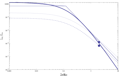
Figure 1: ${\mathcal{L}_{X}/\mathcal{L}_{*}}$ from Eq. (19). Dashed curve: $\Theta_{0}=4.3\times 10^{-4}$; Dotted curve: $\Theta_{0}=1.1\times 10^{-3}$, both for $\lambda=0$ and thus $q=2$ (see text); Solid curve: $\Theta=2.6\times 10^{-3}[(\mathcal{L}_{X}/\mathcal{L}_{*})/(\mathcal{L}_{X}/6.6\times 10^{-7}]^{1/3}$, corresponding to $q=3$. All cases use $q_{\alpha}cos\theta_{s}=0.14$. The dots correspond to the solar average (lower) and maximum (upper) (Peres et al. 2000) and the straight line to the right of $2\pi Ro=0.12$ is the Wright et al. (2011) data fit. Straight lines to the left of this point correspond to $q=0$ (Wright et al. 2011) and $q=0.16$ (Reiners et al. 2014) data fits.

4 Conclusion

Using physical arguments, we have developed a relationship between $\mathcal{L}_{X}/\mathcal{L}_{*}$ and $Ro$. The result accounts for both a transition to $Ro$ quasi-independence at low $Ro$ and a strong inverse dependence at large $Ro$, in general agreement with observations. Our result that the predicted transition toward $Ro$ independence at low $Ro$– is independent of the specific dependence on $Ro$ for $Ro>>1$. Our emergent saturated field strength s for $Ro<<1$ also agrees with the scalings of Christensen (2009), shown to match a range of planetary and stellar dynamo simulations.

Previous attempts to explain the activity–$Ro$ number relation have focused on the possible role of the dynamo number but the expressions commonly used are invalid for $Ro<<1$ limit because the convection turnover time is no longer a good approximation for the turbulent correlation time. When eddies are sheared faster than convection can overturn them, the shear time should replace the convection time when estimating correlation times. We have accounted for this using Eq (9), which reduces to $\tau_{c}$ for $Ro>>1$ and to $\tau_{r}$ for $Ro<<1$. This prescription is widely applicable.

More fundamentally, the dynamo number is insufficient for capturing activity because it does not determine the saturated magnetic field strength. We estimated the latter using a saturation theory rooted in magnetic helicity evolution, combined with a loss of magnetic field by magnetic buoyancy. The associated magnetic flux provides the source of the X-ray luminosity and, when combined with the generalized $\tau_{ed}$ just described, culminates in Eq.(19).

Opportunities for further work abound. Observational constraints on $\lambda$ and on the connection between rotation and internal differential rotation would be desirable in testing Eq.(19).

References

- (1) Blackman E. G., Field G. B., 2002, PRL, 89, 265007
- Blackman & Brandenburg (2003) Blackman E. G., Brandenburg A., 2003, ApJL, 584, L99
- Blackman (2014) Blackman E. G., 2014, Sp. Sci. Rev., doi: 10.1007/s11214-014-0038-6
- (4) Brandenburg A. 2001, ApJ, 550, 824
- Brandenburg (2005) Brandenburg A., 2005, ApJ, 625, 539
- Brandenburg & Sandin (2004) Brandenburg A., Sandin C., 2004, A&A, 427, 13
- (7) Brandenburg A., Subramanian, K. 2005, Phys Rep., 417, 1
- Brummell et al. (2008) Brummell N. H., Tobias S. M., Thomas J. H., Weiss N. O., 2008, ApJ, 686, 1454
- Cattaneo & Tobias (2014) Cattaneo F., Tobias S. M., 2014, ApJ, 789, 70
- Charbonneau (2014) Charbonneau P., 2014, ARA&A, 52, 251
- Christensen, Holzwarth, & Reiners (2009) Christensen U. R., Holzwarth V., Reiners A., 2009, Nature, 457, 167
- Deluca & Gilman (1986) Deluca E. E., Gilman P. A., 1986, GApFD, 37, 85
- Durney & Robinson (1982) Durney B. R., Robinson R. D., 1982, ApJ, 253, 290
- Field & Blackman (2002) Field G. B., Blackman E. G., 2002, ApJ, 572, 685
- Hartmann & Noyes (1987) Hartmann L. W., Noyes R. W., 1987, ARA&A, 25, 271
- Hurlburt, Toomre, & Massaguer (1984) Hurlburt N. E., Toomre J., Massaguer J. M., 1984, ApJ, 282, 557
- Karak et al. (2014) Karak, B. B., Kitchatinov, L. L., & Choudhuri, A. R. 2014, ApJ, 791, 59
- (18) Krause F., Rädler K. H., 1980, Mean Field Magnetohydrodynamics and Dynamo Theory, Pergamon Press
- Markiel & Thomas (1999) Markiel J. A., Thomas J. H., 1999, ApJ, 523, 827
- Micela et al. (1985) Micela G., Sciortino S., Serio S. et al., 1985, ApJ, 292, 172
- (21) Moffatt, H. K. 1978, Magnetic Field Generation in Electrically Conducting Fluids, Cambridge Univ. Press
- Mitra et al. (2014) Mitra D., Brandenburg A., Kleeorin N., Rogachevskii I., 2014, arXiv, arXiv:1404.3194, submitted to MNRAS
- Moreno-Insertis (1986) Moreno-Insertis F., 1986, A&A, 166, 291
- Montesinos et al. (2001) Montesinos B., Thomas J. H., Ventura P., Mazzitelli I., 2001, MNRAS, 326, 877
- Noyes et al. (1984) Noyes R. W., Hartmann L. W., Baliunas S. L., Duncan D. K., Vaughan A. H., 1984, ApJ, 279, 763
- O’Neal et al. (2004) O’Neal D., Neff J. E., Saar S.H. et al. 2004, AJ, 128, 1802
- Pallavicini et al. (1981) Pallavicini R., Golub L., Rosner R. et al. 1981, ApJ, 248, 279
- Parker (1955) Parker E. N., 1955, ApJ, 122, 293
- (29) Parker, E. N. 1979, Cosmical Magnetic Fields: their Origin and their Activity, Clarendon Press, Oxford
- Parker (1993) Parker E. N., 1993, ApJ, 408, 707
- Peres et al. (2000) Peres G., Orlando S., Reale F. et al, 2000, ApJ, 528, 537
- Pevtsov et al. (2003) Pevtsov A. A., Fisher G. H., Acton L. W. et al. 2003, ApJ, 598, 1387
- Pouquet et al. (1976) Pouquet A., Frisch U., Leorat J., 1976, JFM, 77, 321
- (34) Randich, S. 2000, in ASP Conf. Series, Vol. 198, Stellar Clusters and Associations: Convection, Rotation, and Dynamos, ed. R. Pallavicini, G. Micela, & S. Sciortino, 401
- Reiners, Schuessler, & Passegger (2014) Reiners A., Schuessler M., Passegger V.M., 2014, in press ApJ
- Schrijver & Zwaan (2000) Schrijver C.J., Zwaan C., 2000, Solar and Stellar Magnetic Activity, Cambridge University Press
- Shu (1992) Shu F. H., 1992, The physics of astrophysics. Volume II: Gas dynamics, University Science Books, Mill Valley, CA
- Solanki & Unruh (2004) Solanki S. K., Unruh Y. C., 2004, MNRAS, 348, 307
- (39) Subramanian K., Brandenburg A., 2006, ApJL, 648, L71
- Sur, Shukurov, & Subramanian (2007) Sur S., Shukurov A., Subramanian K., 2007, MNRAS, 377, 874
- Thomas, Markiel, & van Horn (1995) Thomas J. H., Markiel J. A., van Horn H. M., 1995, ApJ, 453, 403
- Thomas et al. (2002) Thomas J. H., Weiss N. O., Tobias S. M., Brummell N. H., 2002, Nature, 420, 390
- Tobias (1998) Tobias S. M., 1998, MNRAS, 296, 653
- Tobias et al. (2001) Tobias S. M., Brummell N. H., Clune T. L., Toomre J., 2001, ApJ, 549, 1183
- Vidotto et al. (2014) Vidotto A. A., et al., 2014, MNRAS, 441, 2361
- Vishniac (1995) Vishniac E. T., 1995, ApJ, 451, 816
- Vilhu (1984) Vilhu O., 1984, A&A, 133, 117
- Weber, Fan, & Miesch (2013) Weber M. A., Fan Y., Miesch M. S., 2013, SoPh, 287, 239
- Wright et al. (2011) Wright N. J., Drake J. J., Mamajek E. E., Henry G. W., 2011, ApJ, 743, 48
- Yoshimura (1975) Yoshimura H., 1975, ApJ, 201, 740