Theory of weakly nonlinear self sustained detonations

Abstract

We propose a theory of weakly nonlinear multi-dimensional self sustained detonations based on asymptotic analysis of the reactive compressible Navier-Stokes equations. We show that these equations can be reduced to a model consisting of a forced, unsteady, small disturbance, transonic equation and a rate equation for the heat release. In one spatial dimension, the model simplifies to a forced Burgers equation. Through analysis, numerical calculations and comparison with the reactive Euler equations, the model is demonstrated to capture such essential dynamical characteristics of detonations as the steady-state structure, the linear stability spectrum, the period-doubling sequence of bifurcations and chaos in one-dimensional detonations and cellular structures in multi-dimensional detonations.

1 Introduction

The phenomenon of detonation was discovered in the late ninetheenth century as a supersonic combustion wave that propagates around a thousand times faster than an ordinary flame. The precise nature of detonation was elucidated in the works of Mikhelson, Chapman and Jouguet at the turn of the twentieth century and of Zel’dovich, von Neumann and Döring in the 1940’s (ZND theory, [9, 20]). It was established that a detonation is a shock wave that compresses and heats the reactive gas to temperatures sufficiently high to ignite chemical reactions within a short distance from the shock. Gas expansion caused by the heat release in these reactions creates pressure waves that, on the one hand, support the propagation of the shock and, on the other, accelerate the flow relative to the shock. A self-sustained detonation is possible if such flow acceleration is sufficient to make the flow reach sonic conditions relative to the shock. The presence of a sonic state at some distance from the shock isolates the flow between the shock and the sonic point from the influence of the conditions downstream of the sonic locus, thus making the wave self sustained. Most actual detonations are self sustained and therefore represent an important class of detonations.

In ZND theory, a detonation is assumed to be one-dimensional and in a steady-state in a Galilean frame moving with the wave. The theory is successful in explaining the fundamental nature of a detonation as a coupled shock-reaction zone system. However, in experiments with gaseous detonations, it was observed as early as 1926 that detonations tend to be unsteady and multi-dimensional with rather complex structures and dynamics [37, 9, 20]. To explain these dynamics, theoretical efforts focused on analysis of the stability of ZND solutions began in the 1960’s in the works of Zaidel, Pukhnachev, Schelkin and, most comprehensively, Erpenbeck (see [9] for an early literature review). The theory of linear stability of gaseous detonations was found to be rather involved especially with regard to specific numerical computations for real gaseous mixtures. Much later, Lee and Stewart [19] revisited the stability problem and solved it for an idealized system by employing a relatively straightforward normal-mode approach. Solving the linear stability problem for real complex gaseous mixtures or for systems with losses remains an open problem.

Linear stability theory is successful in predicting, for idealized systems, why and how ZND detonations are unstable to linear perturbations. It is able to predict the neutral stability boundary and the most unstable modes and thus the characteristic length scales of various multi-dimensional structures seen in experiments. However, the predictive power of linear stability theory is limited by its very nature as a linear theory. Gaseous detonations are known to be highly nonlinear and unsteady. The lead shock of such a detonation wave propagates with strong oscillations in its velocity and with a highly non-uniform flow behind the shock that involves additional shocks propagating transversely to the lead shock with triple points forming at their intersection. The triple points in complex detonation waves propagating in tubes with walls covered with soot leave fish-scale traces called detonation cells [37, 20, 9], and these detonations are termed cellular.

Theoretical prediction of the origin and structure of cellular detonations remains an outstanding and challenging open problem. However, some progress has been achieved with use of the tools of asymptotic analysis that allow for insight into the nature of the problem under various limiting conditions. For example, large activation energy [30], small heat-release [32, 4, 5], slow time evolution and small shock curvature [41, 2], weak nonlinearity [29, 3, 27], strong overdrive [5] and other limiting assumptions lead to relatively simple asymptotic models. These asymptotic theories in general describe idealized systems and are thus also limited in their predictive power. Nevertheless, they provide important information about the mechanisms involved in the existence of particular qualitative traits in the real phenomenon.

Two fundamental structural and dynamical properties of gaseous detonations are first that they propagate in a galloping regime in narrow tubes, as characterized by large amplitude pulsations in an essentially one-dimensional wave, and second that the structure of detonation fronts in large channels/tubes or open environments is cellular. From a theoretical point of view, the basic problem is to describe and explain, at least at a qualitative level, the origin and dynamics of these galloping and cellular detonations. Importantly, such detonations have been reproduced and extensively studied in numerical simulations of the reactive Navier-Stokes/Euler equations with simpified descriptions of the chemical reactions and equations of state [25]. Thus, from a modeling standpoint, the use of these equations is frequently appropriate. Some features of pulsating and cellular detonations have been reproduced theoretically in [33, 5]. However, the following questions remain: 1) Can an asymptotic theory predict the observed period-doubling sequence of bifurcations in one-dimensional detonations and the self-sustained cellular structures in two-dimensional detonations? 2) How quantitatively close are the asymptotic predictions to the numerical results from the reactive Navier-Stokes/Euler equations?

Our aim here is to develop a theory that captures the linear and nonlinear dynamics of self sustained detonations, especially with regard to the bifurcation sequence seen in numerical simulations of one-dimensional detonations and the cellular structures found in two-dimensional detonations. Our theory is asymptotic and relies on a number of approximations, namely small heat release, large activation energy, slow time evolution, weak curvature and the Newtonian limit ($0<\gamma-1\ll 1$, where $\gamma$ is the ratio of specific heats). We build on the theory developed in [27, 29] by employing, as an additional approximation, the Newtonian limit (also used in [4] in one spatial dimension for Euler equations) for two-dimensional detonations with retained dissipative effects. The resulting system is a coupled set of three nonlinear partial differential equations. When the dissipative terms are neglected, it is a hyperbolic system for which we compute the traveling wave solutions analogous to ZND waves, their multi-dimensional linear stability properties and full nonlinear dynamics. We provide a quantitative comparison with the results from the reactive Euler equations for all three asymptotic predictions: the steady-state solutions, the linear stability spectrum and the cellular structure. The analysis of the reduced system with retained dissipative effects is postponed for future work.

As we show in Section 3, the two-dimensional reactive Navier-Stokes equations reduce to a forced version of the unsteady, small disturbance, transonic equations (UTSD) given by

$$u_{\tau}+uu_{x}+v_{y} = -\frac{1}{2}\lambda_{x}+\nu u_{xx},$$ (1.1)

$$v_{x} = u_{y},$$ (1.2)

$$\lambda_{x} = -k(1-\lambda)\exp\left(\theta\left(\sqrt{q}u+q\lambda\right)\right),$$ (1.3)

where $u,v$ and $\lambda$ represent leading-order corrections to the $x$ velocity, $y$ velocity and reaction progress variable. The right-hand side of (1.3) is the leading-order contribution of the reaction rate assumed for simplicity to follow a single step Arrhenius kinetics. The parameters $\nu,k,\theta$ and $q$ are the rescaled viscosity, pre-exponential factor, activation energy and heat release, respectively. We find that this reduced asymptotic model captures, at both the qualitative and quantitative levels, not only the ZND structure, but also the linear stability spectrum, the pulsating non-linear dynamics of one-dimensional detonations and the cellular dynamics of two-dimensional detonations.

We also mention the attempts at understanding the nonlinear dynamics of detonations via the use of qualitative models such as those introduced by Fickett [8] and Majda [23]. The idea behind these models is to produce simplified systems that, although not derived from first principles, are capable of reproducing the observed complexity of the solutions of reactive Euler equations while considerably simplifying the analysis. The qualitative models of Fickett and Majda are closely related to the weakly nonlinear theory of detonations developed in [29]. Although these models and the asymptotic theory of Rosales and Majda have enjoyed some success in explaining certain features of different types of traveling wave solutions of reactive Euler/Navier-Stokes equations (i.e., weak and strong detonations), they were shown to lack the necessary complexity needed to reproduce the dynamical properties of real detonations with the rate functions used in prior work [12]. However, simple ad hoc modifications of these models can reproduce much of the complexity of one-dimensional detonations as shown in recent work [26, 15, 7] and also explained in the present work.

The remainder of this paper is organized as follows. In Section 2, we state the main governing equations together with the modeling assumptions regarding the medium and the chemical reactions. In Section 3, we develop an asymptotic approximation of the governing equations and obtain the weakly nonlinear reduced system. We then investigate in Section 4 the possible traveling wave solutions of the asymptotic equations and their linear stability properties. Both the traveling wave solutions and stability spectrum of the asymptotic model are compared with their corresponding results in the reactive Euler system. For the case with no dissipative effects, predictions of the asymptotic model are calculated numerically in Section 5, and a quantitative comparison with the predictions of the reactive Euler equations is presented as well. Finally, in Section 6, we discuss the results as well as point out some remaining open problems.

2 The main governing equations of reactive flow

We assume that the medium is described by the following system of equations expressing, respectively, the laws of conservation of mass, momentum and energy, and the chemical heat release:

$$\frac{\mathrm{D}\rho}{\mathrm{D}t}+\rho\nabla\cdot\mathbf{u} = 0,$$ (2.1)

$$\rho\frac{\mathrm{D}\mathbf{u}}{\mathrm{D}t} = \text{div}\left(\mathbf{T}\right),$$ (2.2)

$$\rho\frac{\mathrm{D}e}{\mathrm{D}t} = \mathbf{T}:\mathbf{D}-\text{div}\left(\mathbf{q}_{e}\right),$$ (2.3)

$$\rho\frac{\mathrm{D}\Lambda}{\mathrm{D}t} = \rho\tilde{W}-\text{div}(\mathbf{q}_{\Lambda}).$$ (2.4)

Here, $\mathrm{D}/\mathrm{D}t=\partial/\partial t+\mathbf{u}\cdot\nabla$ is the material derivative, $\mathrm{v}=1/\rho$ is the specific volume, $\rho$ is the density, $\mathbf{u}$ is the velocity, $\mathbf{T}$ is the Cauchy stress tensor, $\mathbf{D}=\left(\nabla\mathbf{u}+\nabla\mathbf{u}^{T}\right)/2$ is the deformation tensor, $\mathbf{T}:\mathbf{D}=\sum_{i,j}T_{ij}D_{ij}$ is the double contraction of tensors, $e=e_{i}-\tilde{Q}\Lambda$ is the total internal energy per unit mass, $\tilde{Q}$ is the heat release per unit mass, $\mathbf{q}_{e}$ and $\mathbf{q}_{\Lambda}$ represent the flux of energy and species, respectively, $\tilde{W}(\Lambda,T)$ is the rate of reaction and $\Lambda$ is the reaction-progress variable that changes from $\Lambda=0$ in the fresh mixture to $\Lambda=1$ in the fully burnt products.

We make the following standard modeling assumptions (e.g., [40]):

1. The fluid is Newtonian, with the Stokes assumption on the bulk viscosity, so that
   $\mathbf{T}=-\left(p+\frac{2}{3}\mu\text{div}\left(\mathbf{u}\right)\right)\mathbf{I}+2\mu\mathbf{D}$, where $\mu$ is the dynamic viscosity, $p$ is the pressure and $\mathbf{I}$ is the identity tensor.

2. The species flux is given by Fick’s law, $\mathbf{q}_{\Lambda}=\mbox{-$\rho$}d\nabla\Lambda$, with $d$ denoting the diffusion coefficient.

3. The energy flux has contributions from both the heat conduction (given by Fourier’s law) and the species diffusion, so that $\mathbf{q}_{e}=-\kappa\nabla T+\tilde{Q}\rho d\nabla\Lambda$, where $\kappa$ is the heat diffusion coefficient.

4. The medium is a perfect gas described by the ideal-gas equation of state, $p=\rho RT$, with the internal energy given by $e_{i}=p\mathrm{v}/\left(\gamma-1\right)$, where $R$ is the universal gas constant divided by the molecular weight and $\gamma$ is the ratio of specific heats, assumed to be constant.

5. For simplicity, we take the rate of reaction to be $\tilde{W}=\tilde{k}(1-\Lambda)\exp(-\tilde{E}/RT)$, with the added ignition temperature assumption that $\tilde{W}=0$ for $T<T_{i}$ for some temperature, $T_{i}$. Here, $\tilde{k}$ is the rate constant and $\tilde{E}$ is the activation energy. More general rate functions can be considered, in principle, as long as appropriate sensitivity to temperature is preserved.

With these assumptions, we can then rewrite (2.1-2.4) as

$$\frac{\mathrm{D}\rho}{\mathrm{D}t}+\rho\nabla\cdot\mathbf{u} = 0,$$ (2.5)

$$\rho\frac{\mathrm{D}\mathbf{u}}{\mathrm{D}t} = \nabla\cdot\left(-\left(p+\frac{2}{3}\mu\text{div}\left(\mathbf{u}\right)\right)\mathbf{I}+2\mu\mathbf{D}\right),$$ (2.6)

$$\rho\frac{\mathrm{D}e}{\mathrm{D}t} = -p\nabla\cdot\mathbf{u}-\frac{2}{3}\mu\left(\nabla\cdot\mathbf{u}\right)^{2}+\mu\left(\nabla\mathbf{u}:\nabla\mathbf{u}\right)+\mu\left(\nabla\mathbf{u}:\nabla\mathbf{u}^{T}\right)+\nabla\cdot\left(\kappa\nabla T-\tilde{Q}\rho d\nabla\Lambda\right),\qquad$$ (2.7)

$$\rho\frac{\mathrm{D}\Lambda}{\mathrm{D}t} = \mbox{$\rho$}\tilde{W}+\nabla\cdot(\mbox{$\rho$}d\nabla\Lambda).$$ (2.8)

For the analysis that follows, it is convenient to use $e=e_{i}-\tilde{Q}\lambda=RT/(\gamma-1)-\tilde{Q}\Lambda$ to express the energy equation as

$$\rho\frac{\mathrm{D}T}{\mathrm{D}t}-\frac{\gamma-1}{R\gamma}\frac{\mathrm{D}p}{\mathrm{D}t} = \frac{\gamma-1}{R\gamma}\left(\tilde{Q}\rho\tilde{W}-\frac{2}{3}\mu\left(\nabla\cdot\mathbf{u}\right)^{2}+\mu\left(\nabla\mathbf{u}:\nabla\mathbf{u}\right)+\mu\left(\nabla\mathbf{u}:\nabla\mathbf{u}^{T}\right)+\nabla\cdot\left(d\nabla T\right)\right).\qquad$$ (2.9)

We shall focus on the two-dimensional case for simplicity. Consider a localized wave moving into an equilibrium, quiescent state and let $\rho_{a}$, $p_{a}$, $T_{a}$ and $u_{a}=\sqrt{p_{a}/\rho_{a}}$ denote, respectively, the density, pressure, temperature and Newtonian sound speed in the fresh mixture ahead of the wave. We rescale the dependent variables with respect to this reference state. The independent variables are rescaled as follows:

$$x=\frac{X-D_{0}t}{x_{0}},\quad y=\frac{Y}{y_{0}},\quad\tau=\frac{t}{t_{0}},$$ (2.10)

where $X$ and $Y$ are the original spatial variables and $D_{0}$ is a typical wave speed, which is to be determined in the process of deriving the asymptotic model by requiring non-triviality of the leading-order corrections. The length scales, $x_{0}$, $y_{0}$ and the time scale, $t_{0}$, are chosen to reflect the appropriate physics of weakly non-linear waves. We assume that $\epsilon=x_{0}/\left(u_{a}t_{0}\right)$ is small, which means that the spatial scale of interest in the $x$-direction, which is related to the size of the reaction zone, is small compared with the typical distance covered by acoustic waves in time $t_{0}$. For the transverse dimension, we assume the scaling $y_{0}=x_{0}/\sqrt{\epsilon}$ . This follows from the fact that, along a weakly curved front, a distance $\epsilon$ in the normal direction corresponds to a distance $O(\sqrt{\epsilon})$ in the transverse direction.

Several dimensionless groups appear upon rescaling of the governing equations. We define the Reynolds, Pradtl and Lewis numbers, respectively, as follows:

$$\mathrm{Re}=\frac{\rho_{a}u_{a}x_{0}}{\mu},\quad\mathrm{Pr}=\frac{c_{p}\mu}{\kappa},\quad\mathrm{Le}=\frac{\kappa}{\rho_{a}c_{p}d},$$ (2.11)

where $c_{p}=\gamma R/\left(\gamma-1\right)$. Writing $\mathbf{u}=\left(U,V\right)^{T}$, it is convenient to introduce the differential operator:

$$L=\partial_{\tau}+\frac{1}{\epsilon}(U-D_{0})\partial_{x}+\frac{1}{\sqrt{\epsilon}}V\partial_{y}.$$ (2.12)

Introducing the dimensionless parameters,

$$Q=\frac{\tilde{Q}}{RT_{a}},\quad E=\frac{\tilde{E}}{RT_{a}},\quad K=t_{0}\tilde{k}\exp\left(-E\right),$$ (2.13)

the non-dimensional governing equations become:

$$L[\rho]+\rho\left(\frac{1}{\epsilon}U_{x}+\frac{1}{\sqrt{\epsilon}}V_{y}\right) = 0,$$ (2.14)

$$\rho L[U]+\frac{1}{\epsilon}p_{x} = \frac{1}{3\epsilon\mathrm{Re}}\left(U_{xx}+\sqrt{\epsilon}V_{xy}\right)+\frac{1}{\mathrm{\epsilon Re}}\left(U_{xx}+\epsilon U_{yy}\right),$$ (2.15)

$$\rho L[V]+\frac{1}{\sqrt{\epsilon}}p_{y} = \frac{1}{3\epsilon\mathrm{Re}}\left(\sqrt{\epsilon}U_{xy}+\epsilon V_{yy}\right)+\frac{1}{\epsilon\mathrm{Re}}\left(V_{xx}+\epsilon V_{yy}\right),$$ (2.16)

$$\rho L[T]-\frac{\left(\gamma-1\right)}{\gamma}L[p] = \frac{\gamma-1}{\gamma}\left(Q\rho W-\frac{2}{3\epsilon\mathrm{Re}}\left(U_{x}+\sqrt{\epsilon}V_{y}\right)^{2}+\frac{1}{\epsilon\mathrm{Re}}\left(U_{x}^{2}+\epsilon U_{y}^{2}+V_{x}^{2}+\epsilon V_{y}^{2}\right)\right)$$ (2.17)

$$+\frac{\gamma-1}{\gamma}\frac{1}{\mathrm{\epsilon Re}}\left(U_{x}^{2}+\sqrt{\epsilon}U_{y}V_{x}+\sqrt{\epsilon}V_{x}U_{y}+\epsilon V_{y}^{2}\right)+\frac{1}{\mathrm{\epsilon Re}\mathrm{Pr}}\left(T_{xx}+\epsilon T_{yy}\right),\quad\qquad$$

$$\rho L[\Lambda] = \rho W+\frac{1}{\mathrm{\epsilon Re}\mathrm{Pr}\mathrm{Le}}\left(\left(\rho\Lambda_{x}\right)_{x}+\epsilon\left(\rho\Lambda_{y}\right)_{y}\right),$$ (2.18)

where $W$ is defined as

$$W=K(1-\Lambda)\exp\left[E\left(1-\frac{1}{T}\right)\right].$$ (2.19)

3 Weakly nonlinear approximation

We develop an asymptotic simplification of the above general formulation by considering a weakly nonlinear detonation wave, for which we assume that the heat release is small, the activation energy is large and the Newtonian limit, $0<\gamma-1\ll 1$, holds. To be precise, we start from (2.14-2.18) and make the following assumptions:

1. $K=k/\epsilon$, $k=O(1)$. This assumption is chosen to ensure that the reaction rate affects the leading order expansion of $\Lambda$. Since $K=t_{0}\tilde{k}$, this assumption implies that the characteristic time scale, $t_{0}$, of weakly nonlinear detonations is large compared to the collision time, $1/\tilde{k}$, i.e., $t_{0}\sim(1/\tilde{k})/\epsilon$.

2. $\left(\gamma-1\right)Q/\gamma=\epsilon^{2}q$, $q=O\left(1\right)$. This assumption implies that the heat release does not play a role at the linear level. It does not mean that the chemistry is unimportant, but that the heat release must have the appropriate size to balance the nonlinear effects. The extra factor of $\left(\gamma-1\right)/\gamma$ in front of $Q$ arises naturally in the governing equations (see (2.17)) and is retained in the definition of $q$. With the further assumption below of small $\gamma-1$, this implies that $Q$ is $O\left(\epsilon\right)$.

3. $E=\theta/\epsilon^{2},$ $\theta=O\left(1\right)$. This ensures that small temperature deviations – which are $O\left(\epsilon^{2}\right)$ for weak shocks in the Newtonian limit – have an $O\left(1\right)$ influence on the reaction rate.

4. $\gamma-1=\gamma_{1}\epsilon$, $\gamma_{1}=O\left(1\right)$. This assumption is needed to balance the temperature fluctuations with both the acoustics and chemistry at the same order. Without this assumption, the leading order corrections for density, velocity and temperature all behave the same way, as in a weakly nonlinear inert shock [13, 28]. As we show later, having a temperature profile that is different from density/velocity profiles is crucial, as it allows the model derived here to incorporate the dynamical instabilities of detonation waves.

5. $\mathrm{Le}$ and $\mathrm{Pr}$ are $O\left(1\right)$, while $\mathrm{Re}$ is $O(1/\epsilon)$. Other scalings that highlight different transport effects are of course possible, but they are not considered in this work.

To understand some of the intuition behind the asymptotic ordering above, recall the following well-known fact for weak shocks [39]. If the shock strength is measured by the relative jump in pressure across the shock, $\Delta p=\left(p_{s}-p_{a}\right)/p_{a}$ (subscripts $s$ and $a$ denoting post- and pre-shock states, respectively), then the shock Mach number is $\mathrm{M}=1+\left[\left(\gamma+1\right)/(4\gamma)\right]\,\Delta p+O\left(\left(\Delta p\right)^{2}\right)$ and the shock temperature is $T_{s}/T_{a}=1+\left[\left(\gamma-1\right)/\gamma\right]\,\Delta p+O\left(\left(\Delta p\right)^{2}\right)$. Therefore, for weak shocks, with $\mathrm{M}-1=O\left(\epsilon\right)$, in the Newtonian limit, $\gamma-1=O\left(\epsilon\right)$, the leading-order temperature correction is $O\left(\epsilon^{2}\right)$. That is, all variables have an $O\left(\epsilon\right)$ jump across the shock, but the temperature jump is smaller, only $O\left(\epsilon^{2}\right)$. In the chosen asymptotic approximation, we therefore expect similar temperature behavior in the reaction zone as well, at least with inviscid detonations.
Now, we assume the following expansions in the reaction zone:

$$\rho =1+\rho_{1}\epsilon+\rho_{2}\epsilon^{3/2}+\rho_{3}\epsilon^{2}+o(\epsilon^{2}),$$ (3.1)

$$T =1+T_{1}\epsilon+T_{2}\epsilon^{3/2}+T_{3}\epsilon^{2}+o(\epsilon^{2}),$$ (3.2)

$$p =1+p_{1}\epsilon+p_{2}\epsilon^{3/2}+p_{3}\epsilon^{2}+o(\epsilon^{2}),$$ (3.3)

$$\boldsymbol{u} =\mathbf{u}_{1}\epsilon+\mathbf{u}_{2}\epsilon^{3/2}+\mathbf{u}_{3}\epsilon^{2}+o(\epsilon^{2}),$$ (3.4)

$$\Lambda =\lambda+o(\epsilon).$$ (3.5)

The fractional powers appear here because we aim at capturing weak curvature effects in the detonation front. These effects induce a flow velocity transverse to the front, which is $O(\sqrt{\epsilon})$ smaller than the longitudinal velocity. Expansions of this type are standard for waves incorporating the weak-curvature effect (e.g., [17]).

Expanding $p=\rho T$, we find that $p_{1}=\rho_{1}+T_{1}$, $p_{2}=\rho_{2}+T_{2}$ and $p_{3}=\rho_{3}+T_{3}+\rho_{1}T_{1}$. Using these relations to eliminate pressure perturbations, (2.14-2.18) yield

$$\left(-D_{0}\rho_{1x}+U_{1x}\right)+\sqrt{\epsilon}\left(-D_{0}\rho_{2x}+U_{2x}+V_{1y}\right)+$$

$$\epsilon\left(\rho_{1\tau}-D_{0}\rho_{3x}+U_{1}\rho_{1x}+U_{3x}+\rho_{1}U_{1x}+V_{2y}\right) = o(\epsilon),$$ (3.6)

$$\left(-D_{0}U_{1x}+T_{1x}+\rho_{1x}\right)+\sqrt{\epsilon}\left(-D_{0}U_{2x}+T_{2x}+\rho_{2x}\right)+$$

$$\epsilon\left(U_{1\tau}-D_{0}U_{3x}+U_{1}U_{1x}+T_{1}\rho_{1x}+T_{3x}+\rho_{3x}-\rho_{1}\rho_{1x}\right) = \frac{4}{3}\frac{1}{\mathrm{Re}}\left(U_{1}\right)_{xx}+o(\epsilon),$$ (3.7)

$$\left(-D_{0}V_{1x}\right)+\sqrt{\epsilon}\left(-D_{0}V_{2x}+T_{1y}+\rho_{1y}\right)+$$

$$\epsilon\left(V_{1\tau}-D_{0}V_{3x}+U_{1}V_{1x}+T_{2y}+\rho_{2y}\right) = \frac{1}{\mathrm{Re}}\left(V_{1}\right)_{xx}+o(\epsilon),$$ (3.8)

$$\left(-D_{0}T_{1x}\right)+\sqrt{\epsilon}\left(-D_{0}T_{2x}\right)+$$

$$\epsilon\left(T_{1\tau}-D_{0}T_{3x}+U_{1}T_{1x}+\frac{\gamma_{1}}{\gamma}D_{0}\left(\rho_{1x}+T_{1x}\right)\right) = \epsilon q\omega+o(\epsilon),$$ (3.9)

$$-D_{0}\lambda_{x} = \omega+o(1).$$ (3.10)

Because of the weak heat release assumption, we need to expand only the reaction progress variable and the reaction rate to the leading order. As we shall see later, the leading-order corrections to temperature are of order $\epsilon^{2}$, i.e., $T_{1}=T_{2}=0$, and therefore the leading-order reaction rate is given by

$$\omega=k(1-\lambda)\exp\left(\theta T_{3}\right).$$ (3.11)

Balancing $O(1)$ terms, we find that

$$\left[\begin{array}[]{rrrr}-D_{0}&1&0&0\\ 1&-D_{0}&0&1\\ 0&0&-1&0\\ 0&0&0&-1\end{array}\right]\left[\begin{array}[]{r}\rho\\ U\\ V\\ T\end{array}\right]_{1x}=\left[\begin{array}[]{r}0\\ 0\\ 0\\ 0\end{array}\right].$$ (3.12)

This homogeneous system has non-trivial solutions if and only if the coefficient matrix (denoted by $\mathbf{A}$ from now on) is singular. Therefore, we must have $D_{0}=\pm 1$. We focus on a right-going wave for which $D_{0}=1$.

After substituting $D_{0}=1,$ we integrate the first equation in (3.12) to obtain $U_{1}=u(x,y,\tau)+\bar{U}(y,\tau),\ \rho_{1}=u(x,y,\tau)+\bar{\rho}\left(y,\tau\right)$ for some, so far arbitrary, functions $\bar{U}\left(y,t\right)$ and $\bar{\rho}\left(y,t\right)$. In order for our asymptotic expansions to hold as we approach the upstream state, which is assumed to be quiescent and uniform at all times, we require $\rho_{1}=U_{1}\equiv 0$ as $x\to\infty$ (upstream of the wave). As a consequence, it follows that $\bar{U}(y,t)=\bar{\rho}\left(y,t\right)\equiv 0$. Had we considered the case where the wave moves into a non-uniform background, the functions $\bar{\rho}$ and $\bar{U}$ would provide the freedom needed to match the asymptotic expansion in the wave zone to the flow ahead (see, e.g., [29]). A similar reasoning can be used to deduce from the third and fourth equation in (3.12) that $T_{1}=V_{1}\equiv 0$.

At $O(\epsilon^{1/2})$, we obtain

$$\left[\begin{array}[]{rrrr}-1&1&0&0\\ 1&-1&0&1\\ 0&0&-1&0\\ 0&0&0&-1\end{array}\right]\left[\begin{array}[]{r}\rho\\ U\\ V\\ T\end{array}\right]_{2x}=\left[\begin{array}[]{r}0\\ 0\\ -u_{y}\\ 0\end{array}\right],$$ (3.13)

with the same matrix of coefficients, $\mathbf{A}$, as before. Since $\mathbf{A}$ is singular, this system has solutions if and only if the right-hand side is orthogonal to $\mathbf{l}_{0}=\left[1\,1\,0\,1\right]$, which spans the left null-space of $\mathbf{A}$. Clearly, this condition is always satisfied here. Note that from the third and fourth equation in 3.13, we obtain that $V_{2x}=u_{y}$ and $T_{2}=0$, i.e., letting

$$v=V_{2}$$ (3.14)

such that

$$v_{x}=u_{y}.$$ (3.15)

Finally, at $O\left(\epsilon\right)$, we obtain

$$\left[\begin{array}[]{rrrr}-1&1&0&0\\ 1&-1&0&1\\ 0&0&-1&0\\ 0&0&0&-1\end{array}\right]\left[\begin{array}[]{r}\rho\\ U\\ V\\ T\end{array}\right]_{3x}=\left[\begin{array}[]{r}-u_{\tau}-2uu_{x}-v_{y}\\ -u_{\tau}+\frac{4}{3}\frac{1}{\mathrm{\epsilon Re}}u_{xx}\\ -\rho_{2y}\\ q\omega-\frac{\gamma_{1}}{\gamma}u_{x}\end{array}\right].$$ (3.16)

Notice that since $\mathrm{Re}=O(1/\epsilon)$, all terms in (3.16) are $O\left(1\right)$. The solvability condition for this system is that the right-hand side be orthogonal to $\mathbf{l}_{0}=\left[1\,1\,0\,1\right]$, which yields:

$$2u_{\tau}+2uu_{x}+v_{y} = q\omega-\frac{\gamma_{1}}{\gamma}u_{x}+\frac{4}{3}\frac{1}{\mathrm{\epsilon Re}}u_{xx}.$$ (3.17)

This equation together with

$$v_{x} = u_{y},$$ (3.18)

$$\lambda_{x} = -\omega,$$ (3.19)

forms a closed system of equations. The temperature dependence in the leading order rate function, (3.11), can be eliminated by integrating the last equation in (3.16),

$$T_{3}=\frac{\gamma_{1}}{\gamma}u+q\lambda,$$ (3.20)

giving

$$\omega=k(1-\lambda)\exp\left(\theta\left(\frac{\gamma_{1}}{\gamma}u+q\lambda\right)\right).$$ (3.21)

Therefore, we obtain

$$2u_{\tau}+2uu_{x}+\frac{\gamma_{1}}{\gamma}u_{x}+v_{y} = -q\lambda_{x}+\frac{4}{3}\frac{1}{\epsilon\mathrm{Re}}u_{xx},$$ (3.22)

$$v_{x} = u_{y},$$ (3.23)

$$\lambda_{x} = -k(1-\lambda)\exp\left(\theta\left(\frac{\gamma_{1}}{\gamma}u+q\lambda\right)\right).$$ (3.24)

As can be seen from (3.16), species and heat diffusion play no role in the asymptotic equations up to $O\left(\epsilon\right)$. Had we considered different asymptotic orderings for the Lewis and Prandtl numbers, these effects would introduce diffusive terms in the energy and the reaction-rate equations. We consider no such effects in this work and hence the only effective diffusion in the asymptotic model comes from the viscous dissipation.

It is convenient to further rescale the variables as:

$$x\mapsto x-\gamma_{1}/\left(2\gamma\right)\tau,\ y\mapsto 2^{-1/2}q^{-1/4}y,\ \tau\mapsto q^{-1/2}\tau,\ u\mapsto q^{1/2}u,\ v\mapsto 2^{1/2}q^{3/4}v,$$ (3.25)

where the scale for $u$ is chosen so that the traveling wave solution found later in Section 4.1 has speed $1$. We also choose $\epsilon=\left(\gamma-1\right)/\gamma$, which means that $\gamma_{1}=\gamma$. Other choices of $\epsilon$ are possible as long as $\epsilon$ and $\gamma-1$ are of the same asymptotic order when $\epsilon\to 0$. These choices, although equivalent in the limit $\epsilon\rightarrow 0$, will have some effect on the quantitative numerical predictions for finite $\epsilon$. With this rescaling and the choice of $\epsilon$, we obtain our final asymptotic system of equations of weakly nonlinear detonation:

$$u_{\tau}+uu_{x}+v_{y} = -\frac{1}{2}\lambda_{x}+\mbox{$\nu$}u_{xx},$$ (3.26)

$$v_{x} = u_{y},$$ (3.27)

$$\lambda_{x} = -k(1-\lambda)\exp\left[\theta\left(\sqrt{q}u+q\lambda\right)\right],$$ (3.28)

where $\nu=2/\left(3\sqrt{q}\epsilon\mathrm{Re}\right)$ is the dimensionless viscosity coefficient.

In the inviscid case, (3.26-3.28) must be supplemented by the appropriate jump conditions across shocks. If the shock locus is defined by $\phi(x,y,\tau)=x-s(y,\tau)=0$ and $[z]$ denotes the jump of $z$ across the shock, the Rankine-Hugoniot conditions are:

$$s_{\tau}\left[u\right]-\frac{1}{2}\left[u^{2}\right]+s_{y}\left[v\right] = 0,$$ (3.29)

$$s_{y}\left[u\right]+\left[v\right] = 0,$$ (3.30)

$$\left[\lambda\right] = 0.$$ (3.31)

These equations follow from the conservation form of (3.26-3.28).

Implicit in the definition (2.19) of the rate of reaction, $W$, lies the ignition temperature assumption, such that $W\equiv 0$ for $T<T_{i}/T_{a}$. Thus, the leading order reaction rate, $\omega$, given by (3.11) also satisfies $\omega\equiv 0$ for $T_{3}<\left(T_{i}/T_{a}-1\right)/\epsilon^{2}$ or, equivalently, for $u+q\lambda<\left(T_{i}/T_{a}-1\right)/\epsilon^{2}$. In order to prevent reactions from occurring in the ambient state, a reasonable constraint on the ignition temperature is that it be larger than the ambient temperature, $T_{a}$. Furthermore, for the ZND solution to exist, it is necessary that the ignition temperature, $T_{i}$, be smaller than the temperature at the von Neumann state of the ZND solution. In the weakly nonlinear regime considered in this paper, we must therefore have $0<T_{i}-T_{a}=O\left(\epsilon^{2}\right)$. This should be viewed as a modeling assumption about the chemical kinetics. Notice that in the inviscid case, the ignition temperature, if taken to be $T_{i}\gtrapprox T_{a}$, has no effect on the ZND profiles and their stability properties. Simply, it states that the reactions occur only after the shock and therefore, $\omega=0$ ahead of the wave. When considering viscous effects, however, the traveling wave profiles and their dynamical evolution will depend on the ignition temperature and $T_{i}$ should therefore be considered as another parameter that affects the properties of the solutions.

For the convenience of the reader, in Table 1, we collect the relations between various dimensionless and dimensional quantities.

Dimensional	Dimensionless	Physical meaning
$\tilde{Q}$	$Q=\tilde{Q}/RT_{a}=\epsilon q$	Heat release
$\tilde{E}$	$E=\tilde{E}/RT_{a}=\theta/\epsilon^{2}$	Activation energy
$\tilde{k}$	$K=t_{0}\tilde{k}\exp(-E)=k/\epsilon$	Reaction prefactor
$t$	$\tau=t/t_{0}=\epsilon tu_{a}/x_{0}$	Time
$X$	$x=\left(X-D_{0}t\right)/x_{0}-\tau=\left[X-\left(D_{0}+\epsilon u_{0}\right)t\right]/x_{0}$	Longitudinal direction
$Y$	$y=\left(\sqrt{2\epsilon}q^{1/4}/x_{0}\right)Y$	Transverse direction
$\mu,d,\kappa$	$\nu=2/\left(3\sqrt{q}\epsilon\mathrm{Re}\right)$	Dissipative effects

Table 1: Summary of scaling relationships.

The relationships between the asymptotic variables $u$, $v$ and $\lambda$ and the physical (dimensionless, rescaled with the upstream state) quantities, $\rho,\,U,\,V,\,T$ and $\Lambda$ are given by

$$\rho = 1+\epsilon\sqrt{q}u+O(\epsilon^{3/2}),$$ (3.32)

$$U = \epsilon\sqrt{q}u+O(\epsilon^{3/2}),$$ (3.33)

$$V = \epsilon^{3/2}\sqrt{2}q^{3/4}v+O(\epsilon^{2}),$$ (3.34)

$$T = 1+\epsilon^{2}\left(\sqrt{q}u+q\lambda\right)+O(\epsilon^{5/2}),$$ (3.35)

$$\Lambda = \lambda+O(\epsilon).$$ (3.36)

For the remainder of the paper, we focus exclusively on the inviscid case such that the asymptotic equations take the form

$$u_{\tau}+uu_{x}+v_{y} = -\frac{1}{2}\lambda_{x},$$ (3.37)

$$v_{x} = u_{y},$$ (3.38)

$$\lambda_{x} = -k(1-\lambda)\exp\left[\theta\left(\sqrt{q}u+q\lambda\right)\right].$$ (3.39)

We note here that without the chemical reaction, (3.37-3.39) reduce to

$$u_{\tau}+\left(\frac{u^{2}}{2}\right)_{x}+v_{y} = 0,$$ (3.40)

$$v_{x} = u_{y},$$ (3.41)

which are canonical equations appearing in the analysis of various physical phenomena modelled by weakly-nonlinear quasi-planar hyperbolic waves. In terms of the velocity potential, $\phi$, such that $\nabla\phi=\left(u,v\right)$, these equations can be rewritten as

$$\phi_{x\tau}+\left(\frac{\phi_{x}}{2}\right)_{x}^{2}+\phi_{yy}=0,$$ (3.42)

which is the well-known unsteady small disturbance transonic equation [22]. In nonlinear acoustics, this equation is also known as the Zabolotskaya-Khokhlov equation [42].

In the following sections, we investigate the steady-state solutions of (3.37-3.39), their spectral stability and nonlinear dynamics, and demonstrate that the asymptotic theory contains the essential features of not only the steady-state one-dimensional, but also the unsteady and multi-dimensional travelling waves of the reactive Euler equations.

4 Travelling wave solutions and their linear stability

In this section, we analyze the travelling wave solutions of the asymptotic equations and their spectral stability, showing that the asymptotic solutions are analogous to their ZND counterparts. We start by presenting the one-dimensional travelling wave solutions in Section 4.1, which are the basis for the one- and multi-dimensional stability analyses presented in Section 4.2.

4.1 Travelling wave solutions of the asymptotic model

Seeking the one-dimensional travelling wave solutions of the inviscid asymptotic model (3.37-3.39) of the form $\bar{u}=\bar{u}(x-\bar{D}\tau)$, we obtain

$$\bar{u}=\bar{D}+\sqrt{\bar{D}^{2}-\bar{\lambda}},$$ (4.1)

where $\bar{D}$ is the speed of the wave and the bar denotes the steady state. It is easily seen that, for the solution to remain real at the end of the reaction zone, we must choose $\bar{D}\geq 1$. The precise choice of the value is related to the degree of overdrive of the wave. Even though the overdriven detonations can be included in the analysis, we focus on the important case of a self sustained detonation in which the steady state has a sonic point at the end of the reaction zone. Then, $\bar{D}=1$ and

$$\bar{u}=1+\sqrt{1-\bar{\lambda}},$$ (4.2)

where $\bar{\lambda}$ solves

$$\bar{\lambda}_{\xi}=-k\left(1-\bar{\lambda}\right)\exp\left(\theta\left(\sqrt{q}\bar{u}+q\bar{\lambda}\right)\right)$$ (4.3)

with $\xi=x-\tau$ and boundary condition $\bar{\lambda}(0)=0$ (this is analogous to the ZND theory, see [9]). This solution is used in the analysis that follows.

The steady-state structure of the asymptotic model contains substantial information about the underlying modeling assumptions. A crucial qualitative feature of the structure is that, because of the behaviour of the leading order correction to temperature, $T_{3}=u+q\lambda$, it is possible to have a maximum of the reaction-rate function, (4.3), inside the reaction zone, as we show in Fig. 4.1.

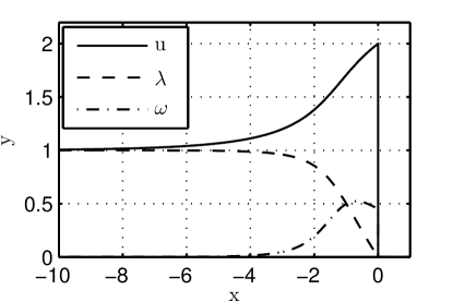
Figure 4.1: Steady-state profiles and the rate function of the asymptotic solution for $q=1.7$ and $\theta=1.7$.

The presence of the internal maximum in the reaction rate appears to be a key factor responsible for the observed unsteady dynamics of real detonations, consistent with our previous work on a closely related model equation [15, 7]. In fact, we have verified that even the qualitative models of Fickett,

$$u_{t}+\left(\frac{u^{2}}{2}+q\lambda\right)_{x} = 0,\qquad\lambda_{t}=\omega(\lambda,u),$$ (4.4)

and Majda (in the inviscid limit),

$$\left(u+q\lambda\right)_{t}+\left(\frac{u^{2}}{2}\right)_{x} = 0,\qquad\lambda_{t}=\omega(\lambda,u),$$ (4.5)

are capable of capturing the one-dimensional instabilities of detonation waves if the reaction rate is taken as (3.21). We recall that, in these models, the reaction rate usually takes the form

$$\omega=\left(1-\lambda\right)\varphi\left(u\right),$$ (4.6)

where the ignition function, $\varphi\left(u\right)$, is

$$\varphi=\begin{cases}\varphi_{0}\left(u\right),&u>u_{i}\\ 0,&u<u_{i}\end{cases},$$ (4.7)

and $u_{i}$ is the “ignition-temperature” parameter (see, e.g., [23, 12]). The new rate function, given by (3.21), reflects the crucially important feature of the heat-release in unstable detonations, which exhibits a maximum inside the reaction zone. Thus, both Fickett’s and Majda’s models possess the necessary complexity needed to capture the qualitative dynamics of one-dimensional unstable detonations provided that the reaction-rate function is chosen appropriately.

The steady-state solution also provides a first quantitative test of the accuracy of the asymptotic approximation. In Fig. 4.2, we show a comparison between the ZND solutions of the reactive Euler equations and their asymptotic counterparts as predicted by the present theory. We see that the asymptotic approximation performs rather well when the heat release is small and the activation energy is large, i.e., when $Q\sim\epsilon$ and $E\sim 1/\epsilon^{2}$. For example, for the realistic value of $\gamma=1.2$ $\left(\epsilon=1/6\right)$, the relative error is only a small percentage (Fig. 4.2(c)). As expected, for the smaller value of $\gamma=1.1$ ($\epsilon=1/11$), the agreement is seen to improve (Fig. 4.2(b,d)), with the maximum relative error approximately two percent of the flow velocity. As expected, the approximation worsens as the values of $\gamma-1$ and $Q$ increase or the value of $E$ decreases.

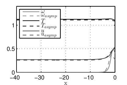
(a) Profiles for $\gamma=1.2,\ Q=0.4,\ E=50$; $\epsilon=1/6$.

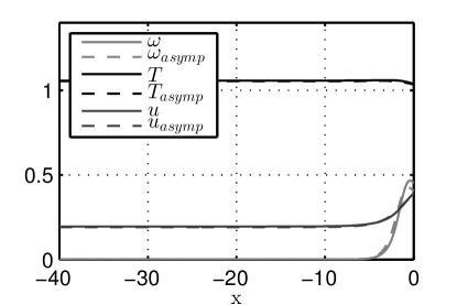
(b) Profiles for $\gamma=1.1,\ Q=0.4,\ E=50$; $\epsilon=1/11$.

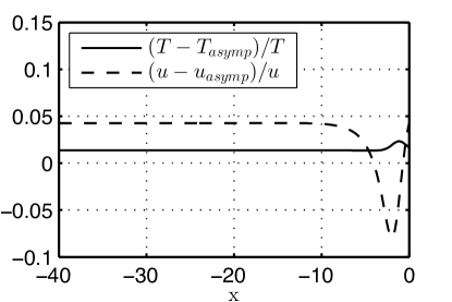
(c) Error for $\gamma=1.2,\ Q=0.4,\ E=50$; $\epsilon=1/6$.

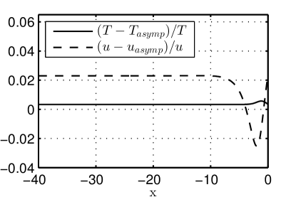
(d) Error for $\gamma=1.1,\ Q=0.4,\ E=50$; $\epsilon=1/11$.

Figure 4.2: Comparison between the exact and asymptotic steady-state ZND profiles. The asymptotic solutions are calculated using (3.32-3.36).

4.2 Linear stability theory for the asymptotic model

With the steady-state solutions in reasonable agreement with the reactive Euler equations, we next investigate their stability properties. It is well known that the reactive Euler equations for the ideal-gas equation of state and simple-depletion Arrhenius kinetics predict that the steady-state detonations are unstable when the activation energy is large enough at a fixed heat release [6, 19, 31]. In this section, we analyze the linear stability of the traveling wave solutions obtained in the previous section to see if the asymptotic theory agrees with the Euler equations in this regard as well. We show that, indeed, the steady-state detonation waves become unstable if either the heat release or the activation energy crosses a certain threshold. We also demonstrate that multi-dimensional effects play a nontrivial role in the onset of instabilities.

To proceed with the analysis, let $\bar{u}$ and $\bar{\lambda}$ be the steady-state solution obtained in Section 4.1. Rewriting (3.37-3.39) in a shock-attached frame, $\chi=x-s(y,\tau)$, where $s(y,\tau)$ is the shock position, we obtain

$$u_{\tau}+\left(u-s_{\tau}\right)u_{\chi}+\frac{1}{2}\lambda_{\chi}+v_{y}-s_{y}v_{\chi} = 0,$$ (4.8)

$$u_{y}-s_{y}u_{\chi}-v_{\chi} = 0,$$ (4.9)

$$\lambda_{\chi} = -k\left(1-\lambda\right)\exp\left(\theta\left(\sqrt{q}u+q\lambda\right)\right).$$ (4.10)

Next, we expand the solution in normal modes,

$$u = \bar{u}(\chi)+\delta u_{1}(\chi)\exp\left(\sigma\tau+ily\right)+O\left(\delta^{2}\right),$$ (4.11)

$$v = \delta v_{1}(\chi)\exp(\sigma\tau+ily)+O(\delta^{2}),$$ (4.12)

$$\lambda = \bar{\lambda}(\chi)+\delta\lambda_{1}(\chi)\exp\left(\sigma\tau+ily\right)+O\left(\delta^{2}\right),$$ (4.13)

$$s = \bar{D}\tau+\delta\exp\left(\sigma\tau+ily\right),$$ (4.14)

and let $\delta\rightarrow 0$. The linearized equations are then

$$\left(\bar{u}-\bar{D}\right)u_{1}^{\prime} = -(\sigma+\bar{u}^{\prime})u_{1}+\sigma\bar{u}^{\prime}-ilv_{1}-\frac{1}{2}\left(g(\chi)u_{1}+h(\chi)\lambda_{1}\right),$$ (4.15)

$$v_{1}^{\prime} = ilu_{1}-il\bar{u}^{\prime},$$ (4.16)

$$\lambda_{1}^{\prime} = g(\chi)u_{1}+h(\chi)\lambda_{1},$$ (4.17)

where the prime denotes a differentiation with respect to $\chi$ and

$$g(\chi) = -\frac{\partial\omega}{\partial u}\left(\bar{u},\bar{\lambda}\right)=-k\theta\sqrt{q}\left(1-\bar{\lambda}\right)\exp\left[\theta\left(\sqrt{q}\bar{u}+q\bar{\lambda}\right)\right],$$ (4.18)

$$h(\chi) = -\frac{\partial\omega}{\partial\lambda}\left(\bar{u},\bar{\lambda}\right)=-k\left[\theta q\left(1-\bar{\lambda}\right)-1\right]\exp\left[\theta\left(\sqrt{q}\bar{u}+q\bar{\lambda}\right)\right].$$ (4.19)

The boundary conditions for (4.15-4.17) are obtained from linearizing (3.29-3.31):

$$u_{1}(0)=2\sigma;\qquad v_{1}(0)=-2il;\qquad\lambda_{1}(0)=0.$$ (4.20)

Noticing that for self sustained detonation, $\bar{u}-\bar{D}\to 0$ as $\chi\rightarrow-\infty$, we require that the right-hand side of (4.15) vanish in the limit as well, i.e.,

$$H(\sigma,l)=-(\sigma+\bar{u}^{\prime})u_{1}+\sigma\bar{u}^{\prime}-ilv_{1}-\frac{1}{2}\left(g(\chi)u_{1}+h(\chi)\lambda_{1}\right)\rightarrow 0\quad\text{as }\chi\rightarrow-\infty.$$

Because $\bar{u^{\prime}}\rightarrow 0,\ g(\chi)\rightarrow 0$ as $\chi\rightarrow-\infty$, this solvability condition (alternatively called the “boundedness” or the “radiation” condition [19]) simplifies to

$$-\sigma u_{1}-ilv_{1}-\frac{1}{2}h\left(-\infty\right)\lambda_{1}\to 0\quad\text{as }\chi\to-\infty.$$ (4.21)

To eliminate the numerical inconvenience of $\sigma=0,\ l=0$ always being an eigenvalue – a consequence of the translation invariance of the traveling wave – we rescale $u_{1}$ and $\lambda_{1}$ by $\sigma$ and $v_{1}$ by $il$. The stability problem is then posed as follows:

Solve

$$\left(\bar{u}-\bar{D}\right)u_{1}^{\prime} = -(\sigma+\bar{u}^{\prime})u_{1}+\bar{u}^{\prime}+\frac{l^{2}}{\sigma}v_{1}-\frac{1}{2}\left(g(\chi)u_{1}+h(\chi)\lambda_{1}\right),$$ (4.22)

$$v_{1}^{\prime} = \sigma u_{1}-\bar{u}^{\prime},$$ (4.23)

$$\lambda_{1}^{\prime} = g(\chi)u_{1}+h(\chi)\lambda_{1},$$ (4.24)

subject to $u_{1}(0)=2,\ v_{1}(0)=-1$ and $\lambda_{1}(0)=0$ at the shock and the boundedness condition (4.21) at negative infinity.

The preceding eigenvalue problem is solved numerically using the shooting method of [19]. We solve the problem for different values of $\theta$, $q$ and $l$, which are the only remaining parameters. Consistent with the behaviour of the stability spectrum of detonation waves in reactive Euler equations [19], we find that unstable modes do exist either for large enough $q$ or for large enough $\theta$. We also find that the transverse modes, where $l\neq 0$, tend to be more unstable than purely longitudinal disturbances [31].

First, we consider the purely one-dimensional problem, i.e., with $l=0$. In Fig. 4.3, we show the contour plot of the absolute value of the stability function,

$$|H\left(\sigma,0\right)|=\left|-(\sigma+\bar{u}^{\prime})u_{1}+\sigma\bar{u}^{\prime}-\frac{1}{2}\left(g(\chi)u_{1}+h(\chi)\lambda_{1}\right)\right|,$$ (4.25)

as a function of real and imaginary parts of $\sigma$. The valleys in the plot of $|H(\sigma,0)|$, which correspond to the darker regions in Fig. 4.3, provide an initial guess for the location of eigenvalues. A root solver is then used wherein the complex function, $H(\sigma,0)$, is set to zero in order to accurately locate the eigenvalues. An increasing number of unstable eigenvalues is seen as the neutral boundary is crossed by increasing the heat release, $q$, for a given value of the activation energy, $\theta$. The qualitative behavior of the spectrum is in agreement with that known for the Euler detonations [19]. Furthermore, Figs. 4.3(a-d) show the migration of the oscillatory complex conjugates, with $\sigma_{i}\neq 0$, into non-oscillatory unstable modes that are also observed in the Euler equations [30]. Finally, in Figs. 4.3(e,f), we see that far into the unstable regime, many eigenvalues are found, indicating a complexity of the linear spectrum.

We also obtain the neutral stability curves for the first two unstable eigenvalues in the asymptotic model, as shown in Fig. 4.4(a). It is seen that the lowest frequency mode $1$ is more unstable than mode $2$ for a wide range of $q$ and $\theta$. Substantially away from the neutral boundary, the non-oscillatory root may become dominant, as is seen in the example shown in Fig. 4.3(c,d).

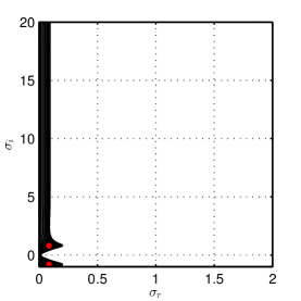
(a) $q=1.8$

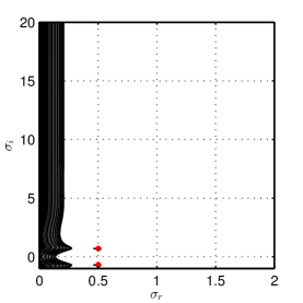
(b) $q=2.2$

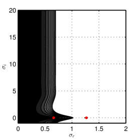
(c) $q=2.6$

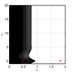
(d) $q=2.75$

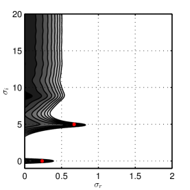
(e) $q=3.5$

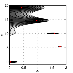
(f) $q=4.5$

Figure 4.3: Contour plots of the spectral function (4.25) for $\theta=1.8$ and increasing $q$. Note that the real part of the non-oscillatory root increases with $q$. The red dots in the figures represent the eigenvalues. In (e) and (c), the dominant non-oscillatory root is not shown.

In Fig. 4.4(b), we plot the neutral curve for the lowest frequency eigenvalue, indicated by the solid line in Fig. 4.4(a), in the plane of the heat release, $Q$, and the activation energy, $E$. The result is compared with the neutral curve computed directly from the reactive Euler equations [19] and a reasonably close agreement between the two is seen. We observe that, as expected, the agreement improves with smaller $Q$ and larger $E$. Finally, since the asymptotic model allows for easy calculations of the high activation energy/small heat release limit, we extend the prediction of the neutral boundary to rather high values of $E\approx 250$ and note that the asymptotic curve follows the scaling $Q\sim 1/E$ very well. In fact, a simple least-squares fitting of the form $Q=c_{1}/E$ gives an $r^{2}$ value of $0.9841$.

(a) Neutral stability boundaries for the first two low-frequency modes in the asymptotic model. The modes are unstable to the right of the curves.

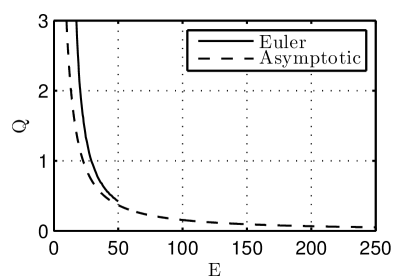
(b) Comparison of the asymptotic and the exact [19] neutral stability boundaries for $\gamma=1.2$, in the heat release, $Q$, versus activation energy, $E$, plane.

Figure 4.4: Neutral stability curves.

If $l\neq 0$, then there is the possibility that transverse waves will trigger the instabilities. This occurs in the Euler equations, where it is found that multi-dimensional instability prevails over purely longitudinal instability. Again, using the shooting method, we solve (4.22-4.24) numerically for various values of $l$. Solving for the roots of the radiation function,

$$H(\sigma,l)=-(\sigma+\bar{u}^{\prime})u_{1}+\sigma\bar{u}^{\prime}-ilv_{1}-\frac{1}{2}\left(g(\chi)u_{1}+h(\chi)\lambda_{1}\right),$$ (4.26)

at $\chi=-\infty$, we obtain the two-dimensional stability spectrum. We first fix $q=1.7$ and vary $\theta=1.65,\,1.60,\,1.55$. In Fig. 4.5, we show the real and imaginary parts of the unstable modes for relatively small values of $l$. It is seen that the model predicts purely two-dimensional instabilities for a certain range of the transverse wave numbers, and that increasing the activation-energy parameter, $\theta$, has a destabilizing effect on the steady-state solutions.

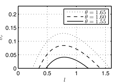
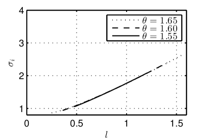
Figure 4.5: Growth rate and frequency for the most unstable mode versus the wave-number, $l$, for several values of the activation energy, $\theta$.

We also perform a quantitative comparison between the two-dimensional stability of the asymptotic model and the known stability diagram for the Euler equations. We choose the values of $\gamma=1.2,\ Q=0.4$ and $E=50$. Then, after performing the appropriate conversion between dimensionless variables, we compare the asymptotic results with those obtained in [36] (see Fig. 4.6). We observe a fair agreement. There are, however, some differences. We see that for the parameters chosen in Fig. 4.6, the asymptotic model predicts one-dimensional instabilities, while the reactive Euler equations do not. Also, we observe that the disagreement between the imaginary parts of the eigenvalues increases with increasing wavenumber. This should be expected because short transverse wavelengths cannot be represented accurately in the weak curvature limit assumed for this model. In the next section, we investigate the long-time non-linear dynamics of the asymptotic solutions in regimes corresponding to linearly unstable steady-state one-dimensional solutions. The calculations are performed in both one and two spatial dimensions.

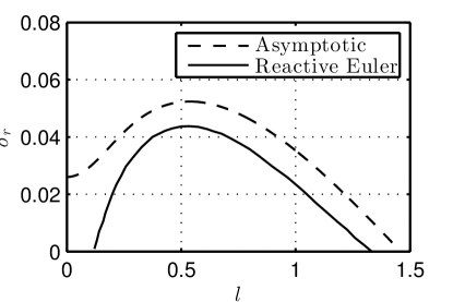
Figure 4.6: Comparisons of the growth rate and frequency for the most unstable mode versus the wave number, for $Q=0.4$ and $E=50$. The dashed curve corresponds to the model in this paper. The solid line corresponds to the reactive Euler equations as computed in [36].

5 Nonlinear dynamics of the asymptotic model

In the previous section, we showed that the asymptotic model exhibits the same linear stability behavior as the reactive Euler equations. The question of what happens after the onset of instabilities can be investigated through direct numerical simulations of the model equations. We show below that the traveling wave solutions of the asymptotic model reproduce, in both one and two spatial dimensions, the complexity observed in solutions of the reactive Euler equations.

5.1 Galloping detonations

We focus here on the ability of the asymptotic model to predict the complex nonlinear dynamics of pulsating (galloping) detonations. We perform a detailed numerical investigation of the large time asymptotic behaviour of oscillatory solutions of the model. In the one-dimensional inviscid case, the system given by (3.26-3.28) reduces to

$$u_{\tau}+uu_{x} = -\frac{1}{2}\lambda_{x},$$ (5.1)

$$\lambda_{x} = -k(1-\lambda)\exp(\theta(\sqrt{q}u+q\lambda)).$$ (5.2)

This system resembles the one derived in [29] with one crucial difference – as a consequence of the $\gamma-1=O(\epsilon)$ assumption, the reaction rate function in (5.2) has a more complicated $\lambda$-dependence, which is in fact at the heart of the complexity of the solutions obtained here. System (5.1-5.2) is also the same as in [4], where the $\gamma-1=O(\epsilon)$ assumption is used.

We solve (5.1-5.2) numerically in a shock-attached frame [16], using a second-order finite volume scheme with a second-order Total Variation Diminishing (TVD) Runge-Kutta temporal discretization [21]. Because no differentiation across the shock is performed, true second-order convergence is obtained for the cases tested, which include the convergence to various stable steady-state ZND solutions. We further verified the numerical algorithm by performing a cross-validation between the linear stability solver and the direct numerical solver. That is, we made sure that for several values of $q$, the linear stability prediction of the neutral boundary agrees with the neutral stability boundary of the numerical scheme for the nonlinear model. For example, when $q=1.7$, the linear stability curve in Fig. 4.4(a) indicates that $\theta_{c}=1.710$ is the neutral value of the activation energy, i.e., the ZND wave is unstable for $\theta>\theta_{c}$ and stable for $\theta<\theta_{c}$. Numerical simulations of (5.1-5.2) with $\theta$ slightly above and slightly below $\theta_{c}$ confirm this prediction, as shown in Fig. 5.1, where the shock state, $u_{s}$, is plotted as a function of time.

(a) Stability of the ZND solution at $\theta=1.705<\theta_{c},\ q=1.7$.

(b) Instability of the ZND solution and the limit-cycle attractor at $\theta=1.715>\theta_{c},\ q=1.7$. Notice that the amplitude of the limit cycle scales roughly as the distance to the bifurcation point, as in a super-critical Hopf bifurcation.

Figure 5.1: Nonlinear dynamics of (5.1-5.2) near the neutral boundary, $\theta_{c}=1.710$, as predicted by the linear stability theory for $q=1.7$.

We also compute solutions of (5.1-5.2) further away from the neutral boundary in order to check if the model captures a sequence of bifurcations leading to chaos as occurs in the reactive Euler equations [24, 11]. Such a sequence of bifurcations is indeed present in the model. Long time simulations show that the solutions tend to either a fixed point, a limit cycle or (what appears to be) a chaotic attractor. We run the simulations at $q=5$ and plot the post-shock state, $u_{s}$ (by the Rankine-Hugoniot conditions, $u_{s}=2D$, where $D$ is the shock speed), as a function of time for several different types of solution, as shown in Fig. 5.2. Beyond the stability boundary, the shock velocity becomes oscillatory. Near the neutral boundary, the oscillations have a small amplitude and are periodic (Fig. 5.2(a)), but the structure of each period becomes more complex as we move away from the neutral boundary by increasing the activation energy (Fig. 5.2(b,c)). Eventually, a value of $\theta$ is reached at which no obvious period is evident as seen in Fig. 5.2(d).

(a) $\theta=0.75$

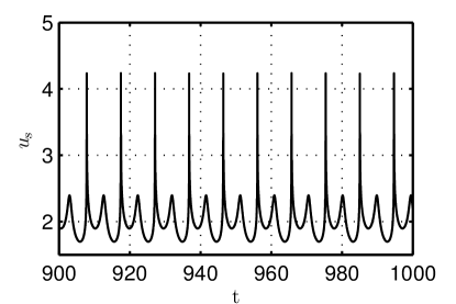
(b) $\theta=0.8$

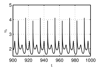
(c) $\theta=0.83$

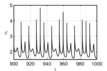
(d) $\theta=0.85$

Figure 5.2: The shock state as a function of time for increasing values of $\theta$ and fixed $q=5$ showing pulsations of different complexity.

The behaviour described in the previous paragraph can be understood in terms of a period doubling sequence of bifurcations where the period becomes longer and more complex with each bifurcation. In order to construct a bifurcation diagram illustrating this process, we proceed as follows: for each value of $\theta$, we follow the evolution of the solution until it settles on the attractor. Then, we extract the set of local minima for $u_{s}(\tau)$ – a finite set for any periodic solution. The values of these minima are then plotted versus the bifurcation parameter, $\theta$. The result is shown in Fig. 5.4, which is reminiscent of the standard Feigenbaum period doubling cascade leading to chaos [34].

It is important to note that the further we move into the unstable region, the harder it is to numerically capture the wave dynamics with good accuracy. That is, in the highly unstable regime ($\theta\gtrapprox 0.85$ in Fig. 5.4), the quantitative details of the bifurcation diagram are sensitively dependent on the grid resolution. In a truly chaotic regime, such sensitivity is intrinsic and reflects the nature of the system. However, another reason, which is at play even before the apparently chaotic regime sets on, is that the wave dynamics can involve spatial scales that undergo large changes (by orders of magnitude) during the wave evolution. This is a direct consequence of the Arrhenius exponential dependence of the reaction rate, which can trigger large variations in the reaction rate from moderate changes in the temperature when the activation energy is large. This issue of stiffness associated with high-activation energy detonations in unstable regimes is discussed next in more detail.

In theoretical and numerical studies of detonation, a widely used spatial scale is taken to be the half-reaction length, $x_{1/2}$, defined as the distance from the shock where half of the energy is released in the ZND solution. The space is then non-dimensionalized, as done in this work, so that the half-reaction happens over a unit length. The numerical resolution is thus measured as a number of points per this unit of length. Although appropriate for stable or weakly unstable detonations, the ZND half-reaction length and therefore the resolution measured on this scale become less meaningful when considering unstable detonations at high activation energies. The reason is that the energy release can become extremely localized during the dynamical evolution of pulsating waves and therefore the actual number of grid points used to capture the heat release region can significantly decrease.

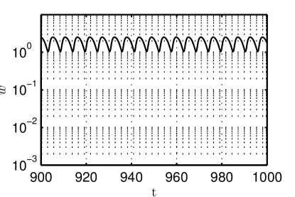
(a) $\theta=0.75$

(b) $\theta=0.8$

(c) $\theta=0.83$

(d) $\theta=0.85$

Figure 5.3: The width of the reaction zone as a function of time. The simulations were performed in a domain of length $L=30$ and with $N=30,000$ grid points ($dx=10^{-3}$).

In order to provide a more quantitative measure of the variations of relevant spatial scales during the time evolution of a pulsating detonation, we introduce the width of the reaction zone as the smallest value, $w_{m}$, such that there exists an interval, $\mathcal{I}$, of length $w_{m}$, where $m$ percent of the energy is released. For nice enough rate functions, $w_{1/2}$ of the ZND solution is roughly equivalent to the half-reaction length, $x_{1/2}$. Notice, however, that for chemical reactions with large induction zones and/or localized heat release, the values of $w_{1/2}$ and $x_{1/2}$ are significantly different, with $w_{1/2}$ becoming a more relevant spatial scale. In the calculations below, we use $m=0.95$ such that $w_{0.95}$ represents, at a given time, the smallest width containing $95\%$ of the heat release.

In Fig. 5.3, we show $w_{0.95}$ as a function of time during the detonation evolution. We fix the numerical resolution at $1000$ points per half-reaction length ($dx=0.001$), which may be considered an overkill for a steady ZND wave. We then compute $w_{0.95}$ as a function of time at different activation energies. As can be seen in Fig. 5.3(a), in the weakly unstable regime, the width of the heat-release zone changes by a factor of about two during the time evolution of the wave; the heat release region is still well resolved. Further into the unstable regime (Fig. 5.3(b,c)), we see that the relevant size of the reaction zone can shrink by more than an order of magnitude and, thus, even with $1000$ points per half-reaction length, there are times when only about $30$ points are used to resolve the heat-release region. If we increase the activation energy even further, stepping into the apparently chaotic regime, we observe very short windows of time when only about $10$ points are being used per heat-release zone.

Figure 5.4: The bifurcation diagram at $q=5$ showing the local minima of the attractor solution’s shock value, $u_{s}(\tau)$, as a function of the activation energy, $\theta$. The simulations were carried out at $N=15,000$ (red) and $N=30,000$ (black) grid points on the computational domain of length $L=30$. Away from the chaotic regimes, the predictions are seen to be nearly identical.

Because of the difficulties outlined above, without resorting to adaptive mesh refinement, $500-1000$ points per half-reaction length are needed to obtain a bifurcation diagram with features that are essentially grid independent away from the chaotic regimes (see Fig. 5.4). While recognizing that such sensitivity to initial conditions or discretization errors is natural for chaotic dynamics, caution is still required when interpreting the results of numerical simulations of unstable detonations with high activation energies.

5.2 Cellular detonation

Multi-dimensional instability is very important in gaseous detonations and results in cellular structures involving triple-point interactions on the detonation lead shock [25, 9, 20]. It is therefore crucial to check if the asymptotic model, (3.26-3.28), can reproduce the dynamics of not only one-dimensional, but also multi-dimensional detonations. As we have seen in Section 4.2, multi-dimensional instabilities can be dominant in the asymptotic model, with the dispersion relation showing a maximum growth rate for some nonzero transverse wave number $l$ (see Fig. 4.5). In this section, we calculate the long-term dynamics of detonation waves when two-dimensional effects are present. In particular, we show that the asymptotic model retains the essential complexity required to reproduce multi-dimensional cellular patterns. Solving (3.37-3.39) numerically turns out to be a non-trivial task and requires special care. In the following subsection, we present a discussion of the algorithm employed in this work.

5.2.1 Numerical algorithm for the two-dimensional asymptotic system

In order to appreciate the subtlety associated with (3.37-3.39), we note that the equations comprise a nonlinear hyperbolic system with one of its characteristic planes orthogonal to time. This means that:

• The initial data are given on a characteristic surface, the $x-y$ plane. The absence of a time derivative in (3.27-3.28) requires the initial conditions to satisfy $v_{x}=u_{y}$, $\lambda_{x}=\omega\left(\lambda,u\right)$.

• Evolving in $\tau$ is a nonlocal procedure and, in the presence of a shock, care has to be taken to avoid spurious numerical oscillations.

Many existing numerical methods for solving (3.40-3.41) are based on a formal rewriting of the system as a single equation,

$$u_{xt}+\left(\frac{u^{2}}{2}\right)_{xx}+u_{yy}=0,$$ (5.3)

by cross-differentiation and substitution. Two concerns arise with this approach. First, the validity of such a transformation is not obvious when $u$ and $v$ are discontinuous functions. Second, in the presence of chemical reactions, differentiation of (3.37) with respect to $x$ produces a delta forcing at the ignition-temperature locus due to the discontinuous nature of the reaction rate. Thus, the techniques based on solving (5.3) are inadequate for our purposes.

Another common technique is to solve for the potential, $\phi$, that satisfies

$$\phi_{x\tau}+\left(\frac{\phi_{x}}{2}\right)_{x}^{2}+\phi_{yy}=0.$$ (5.4)

Again, when chemical reactions are present, complications arise because the reaction rate now becomes an exponential function of $\phi_{x}$ and the discretization errors in $\phi_{x}$ therefore exponentially amplify, requiring very high-order methods for good accuracy.

The method we employ here is based on a direct semi-implicit discretization of (3.26-3.27) following some of the ideas found in [14]. In this method, all terms except for $v_{y}$ are treated explicitly. By chosing second-order spatial and temporal discretizations, we obtain an algorithm that is formally second order in time and space. The general procedure is outlined here to explain our reasoning for the choice of the algorithm.

Assuming that the solution at time $\tau=\tau^{n}$ is known, we evolve it to $\tau=\tau^{n+1}$ as follows:

1. First, we employ a semi-implicit time discretization, where the $v_{y}$ term is treated implicitly. The motivation for this comes from the fact that some waves propagate infinitely fast in the $x-y$ plane. In the simple case of a forward Euler time discretization, we obtain

   $$\frac{u^{n+1}-u^{n}}{\Delta\tau}+(F^{n}(u))_{x}+v_{y}^{n+1} = \lambda_{x}^{n},$$ (5.5)

   $$v_{x}^{n+1} = u_{y}^{n+1},$$ (5.6)

   $$\lambda_{x}^{n+1} = \omega\left(\lambda^{n+1},u^{n+1}\right),$$ (5.7)

   where $F(u)=u^{2}/2$. A more quantitative reason for treating $v_{y}$ implicitly can be seen from the von Neumann stability analysis of the linearized system without chemical reactions, wherein a fully explicit scheme can be unstable (see Appendix A for details).

2. We approximate the explicit terms $\lambda_{x}^{n}$ and $F_{x}^{n}$ using a shock-capturing scheme, e.g., finite volume or ENO/WENO algorithms [21].

3. Using (5.6), we write a forward difference representation of $v_{i,j}^{n+1}$ in terms of $u_{i,j}^{n+1}$ and $u_{i^{\prime},j}^{n+1}$ for $i^{\prime}>i$. For instance, a first-order forward difference scheme can be used, i.e.,

   $$v_{i,j}^{n+1}=v_{i+1,j}^{n+1}-\Delta x\left(u_{i,j}^{n+1}\right)_{y},$$ (5.8)

   where the $y$ derivative approximation is postponed until the next step. The use of the forward difference here is a consequence of up-winding the infinitely fast waves propagating from right to left.

4. Approximate the $y$ derivatives, e.g., by centered differences, to obtain the fully discrete scheme:

   $$u_{i,j}^{n+1} = u_{i,j}^{n}+\Delta\tau\left[-\frac{1}{2}\left(\lambda_{x}\right)_{i,j}^{n}-\left(F_{x}\right)_{i,j}^{n}-\frac{1}{2\Delta y}\left(v_{i,j+1}^{n+1}-2v_{i,j}^{n+1}+v_{i,j-1}^{n+1}\right)\right],$$ (5.9)

   $$v_{i,j}^{n+1} = v_{i+1}^{n+1}-\frac{\Delta x}{2\Delta y}\left(u_{i,j+1}^{n+1}-u_{i,j}^{n+1}+u_{i,j-1}^{n+1}\right).$$ (5.10)

5. In order to solve (5.9-5.10), sweep from right to left, assuming the right boundary values of $u$ and $v$ are known at all times, in the following way:

   1. For some fixed $i$, insert (5.10) into (5.9) and solve the linear system for the vector $u_{i,j}^{n+1}$.

   2. With $u_{i,j}^{n+1}$ find $v_{i,j}^{n+1}$ using (5.9).

   3. Repeat (a),(b) with $i=i-1$ until the left boundary is reached.

6. Finally, compute $\lambda^{n+1}$ by solving (5.7) with a boundary condition on the right of the domain, which is given by

   $$\lambda_{x}^{n+1}(x_{right},y)=0.$$ (5.11)

   Notice that (5.7) is actually an initial value problem for $\lambda^{n+1}$ for fixed $y$ wherein $-x$ is a time-like direction. It can be solved with any initial value solver (e.g., a Runge-Kutta method) if desired.

It may seem counterintuitive at first that the simplified model requires a semi-implicit method while the reactive Euler equations can be solved explicitly. The reason is that the asymptotic approximation is performed in a limit where the reactive Euler equations themselves would have to be treated implicitly. In order to understand this, we look at the three waves present in the Euler equations. Since the weak heat release approximation implies that the detonation velocity is nearly acoustic, and an acoustic wave induces no flow behind it, we see that the speed of the forward acoustic characteristic, given by $u+c-D$ in a frame moving with the wave, is actually an $O\left(\epsilon\right)$ quantity ($D\approx c$ and $u\approx\epsilon$). The entropy and backward acoustic characteristics, on the other hand, have $O\left(1\right)$ speeds. In the asymptotic model, a slow time, $\tau$, is chosen so that the dynamics happen on $O\left(1\right)$ time scales and therefore some characteristics have speeds of $O\left(1/\epsilon\right)$ in the slow time variable. When an explicit method is used to solve the Euler equations in this limit, a typical CFL condition would require a time step, $\Delta\tau\sim\epsilon\Delta x$, and as $\epsilon\to 0$, it becomes clear that the time step restriction becomes unattainable and an implicit method is needed.

The infinite characteristic velocity arises because the $x,y$ plane is a characteristic surface for the equations. A simple rotation in space-time "resolves", to some extent, this issue such that in the "rotated" space-time the system behaves as a standard system of conservation laws. The trade-off for recovering a classical hyperbolic system with finite wave speeds is that one must now consider a grid with moving boundaries. This idea can be exploited to produce fully explicit schemes as shown in [35] for the case without reactions.

5.2.2 Two-dimensional cellular detonations

Using the algorithm described in the previous section, we solve (3.37-3.39) in a frame moving with constant speed, $D_{0}=1$. All simulations are initialized with the one-dimensional ZND solutions obtained in Section 4.1. We then investigate, in the context of the asymptotic equations: 1) the effect of the width of the channel on nonlinear stability properties of the travelling wave solutions; 2) the effect of the periodic boundary conditions; and 3) the effect of increasing heat relase on the wave dynamics.

In Fig. 5.5, we show the profile of $u$ at $\tau\approx 500$ for varying widths of the domain, $L_{y}$, in the $y$ direction. The $y$ boundaries are modelled as rigid walls, appropriate for a detonation in a two-dimensional channel (i.e., a channel with negligible depth). The parameters are fixed at $q=1.7$ and $\theta=1.65$, for which the linear stability calculation shows that the ZND wave is unstable only to two-dimensional perturbations. In a channel of width $L_{y}=2$, the ZND wave remains stable, as seen in Fig. 5.5(a), as the spacing is too narrow for the two-dimensional instability to develop. Increasing the width of the channel, however, allows for a number of transverse modes to be excited, leading to the formation of a multi-dimensional cellular pattern as shown in Figs. 5.5(c,d). The cell size appears to remain around $10$ in all Figs. 5.5(b-d).

When we replace the solid wall boundary conditions with periodic conditions, we observe a two-dimensional version of a spinning detonation. There is only one family of transverse shock waves that all propagate in the same direction. Such a wave can be imagined to form in a narrow gap between two concentric cylindrical tubes, as in a rotating detonation engine [37]. A snapshot of the solution field, $u$, is shown in Fig. 5.6, where relatively strong transversely propagating shocks can be seen.

(a) $L_{y}=2$

(b) $L_{y}=10$

(c) $L_{y}=50$

(d) $L_{y}=100$

Figure 5.5: Dynamics of the asymptotic model in channels of different widths. The plots show the asymptotic variable $u$. The parameters are $q=1.7$, $\theta=1.65$, as in Fig. 4.5. The white region corresponds to the ambient state ahead of the wave, with $u=0$.

Figure 5.6: Detonation in a channel of width $L=100$ with periodic boundary conditions. Parameters are $q=1.7$ and $\theta=1.65$.

(a) $q=1.7$

(b) $q=1.8$

(c) $q=1.9$

(d) $q=2.5$

Figure 5.7: Dynamics of the asymptotic model for varying heat release at a fixed width $L=100$ and activation energy $\theta=1.65$.

In Fig. 5.7, we show the effect of the heat release on the solution structure. We fix $\theta=1.7$ and increase the value of $q$ from $1.7$ to $2.5$. Consistent with the behaviour of detonations in the reactive Euler equations, regular cells are observed at small $q$, as in Figs. 5.7(a,b), but with increasing $q$, the structure of the detonation front becomes more complex with the formation of irregular cells as in Fig. 5.7(d).
All of the previous results show that, at least at a qualitative level, the asymptotic model captures many important characteristics of multi-dimensional detonations. Next, we investigate how quantitatively close the predictions are to the solutions of the reactive Euler equations. The numerical simulations of the reactive Euler equations were carried out using PyCLAW [18], which provides, among other things, a Python wrapper for the classic routines in CLAWPACK. The software requires the user to provide a Riemann solver. We use a Roe-linearized Riemann solver with a Harten-Hyman entropy fix [21]. The classic package of PyCLAW employs a second-order finite volume algorithm with a fractional step method for the time evolution [21]. For the numerical simulations, the reactive Euler equations were non-dimensionalized in the conventional form by the ambient state with velocities scaled by $u_{a}=\sqrt{p_{a}/\rho_{a}},$ spatial variables scaled by the half-reaction length, $x_{1/2}$, and time by $u_{a}/x_{1/2}$.
In Fig. 5.8, we show a comparison between the asymptotic solutions and the solutions of the reactive Euler equations. The parameters chosen are the same as in Fig. 4.6(b), i.e., $\gamma=1.2$, $Q=0.4$ and $E=50$, which in the asymptotic variables are given by $q=2.4$ and $\theta=50/36\approx 1.389$. We start both simulations with the ZND solution and solve for a time interval large enough such that instabilities have already fully developed. Notice that since the asymptotic model uses the slow time variable, $\tau$, we only need to solve it for a relatively short time interval, $\tau\approx 100$. The reactive Euler system, on the other hand, was non-dimensionalized in the conventional way using the regular time variable, $t$, and thus we must solve the system up to $t\approx\tau/\epsilon=600$. We perform all necessary scaling conversions between the variables so that the lengths and amplitudes shown in Fig. 5.8 are consistent. The length of the $y$ domain is fixed in the asymptotic model to be $20$, which corresponds to a length $27.83$ in the regular dimensionless $y$, while the $x$ domain is of length $40$.

(a) Density field, $\rho=1+\epsilon\sqrt{q}u$, as predicted by the asymptotic model.

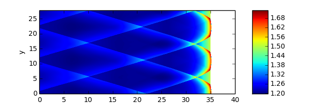
(b) Density field computed from the reactive Euler equations.

Figure 5.8: Comparison between asymptotic and full solutions of the reactive Euler equations for a cellular detonation in a channel.

We see from Fig. 5.8 that the asymptotic model captures the salient features of multi-dimensional detonations with good quantitative agreement. The characteristic scales of the detonation cells are seen to be close. A small difference in the transverse propagation velocity of the triple points is apparent, in the asymptotic case the speed being higher. The transverse shocks in the asymptotic solutions far from the lead shock are seen to be smoother than in the full solutions, which is due to a larger numerical diffusion in the algorithm for the asymptotic model.

Finally, we remark that weakly nonlinear detonations operate in the same fluid dynamic regime as weak shock wave focusing or weak shock reflection at near grazing incidence. As pointed out by von Neumann [38], in this limit the "classical" Mach triple point shock structure is impossible. Yet, both experiments and numerical calculations [10] consistently exhibit triple shock structures in this regime. This apparent contradiction is known as the "von Neumann paradox". Although the structures behind the lead shock in our calculations resemble the triple-points observed in detonations (Fig. (5.9)), a simple algebraic argument can show that the asymptotic equations do not admit “classical” triple points, where three shocks separated by smooth flows meet [35, 14]. Thus, much like in the problem of weak shock reflection, the observed cells in the weak heat release detonations considered in this work present yet another instance of the “von-Neumann paradox”. Here, we make no attempt to address this problem and simply note that triple-point-like structures appear in our numerical simulations behind the lead shock; whether they are true discontinuities, sharp waves or some singularities remains an open problem.

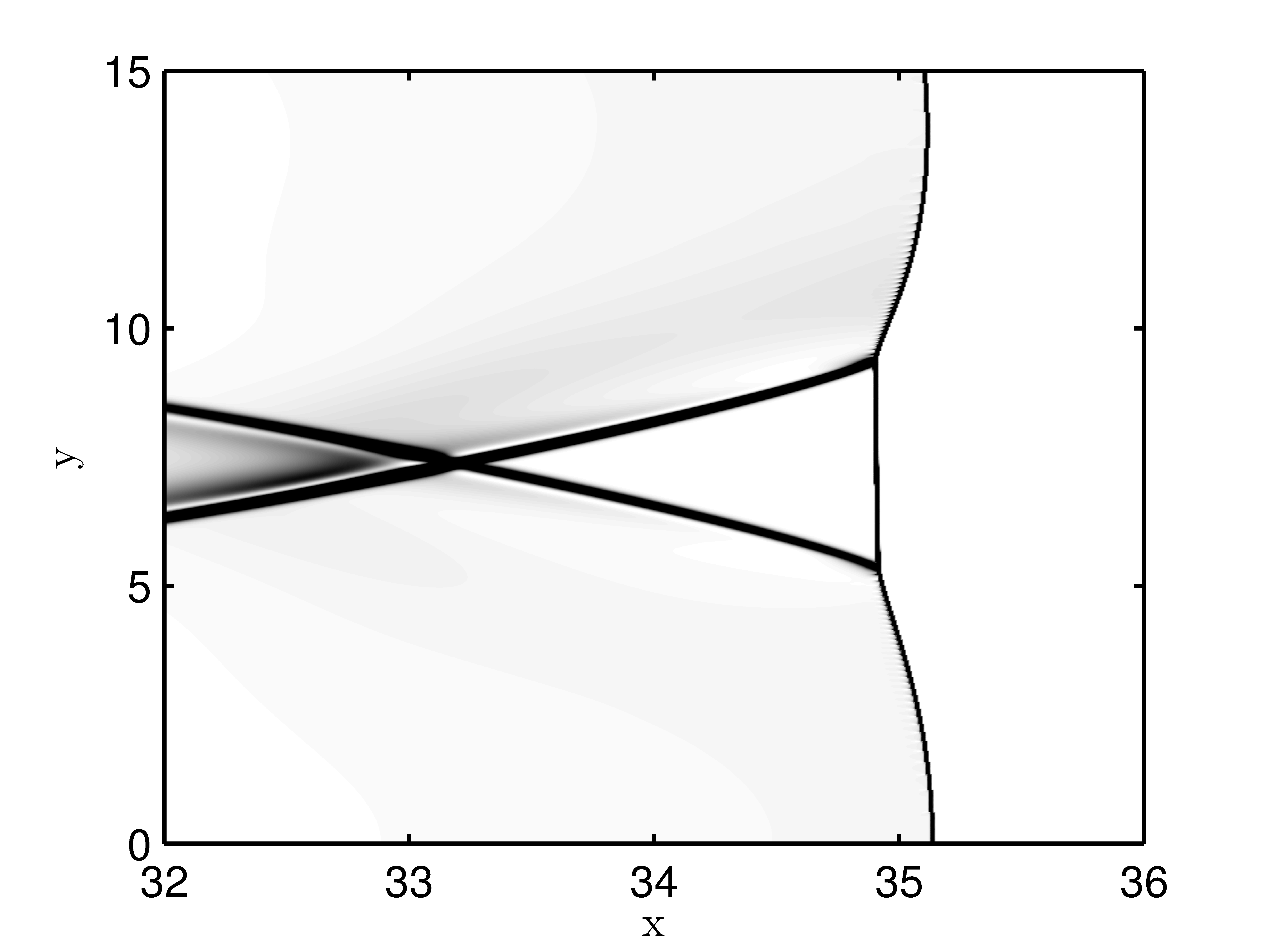
Figure 5.9: Triple-point-like structures in the asymptotic solution of the weakly nonlinear detonation as shown by the magnitude of the density gradient.

6 Discussion and conclusions

In this work, we develop an asymptotic theory of multi-dimensional detonations within the framework of the compressible Navier-Stokes equations for a perfect gas reacting with a one-step heat-release law. The main outcome is a reduced model that consists, in two spatial dimensions, of a forced Burgers-like equation coupled with a heat release equation and an equation that enforces zero vorticity. After specializing the model to the case without dissipative effects, we have analyzed it in detail and have shown that it captures many of the dynamical features of detonations in reactive Euler equations. These include: 1) existence of steady-state travelling waves (i.e., ZND solutions), 2) linear instability of the ZND solutions, 3) existence of a period-doubling bifurcation road to chaos in the one-dimensional case, and 4) onset of cellular detonations in the two-dimensional case. Our theory considers weakly nonlinear detonations in the distinguished limit of small heat release, large activation energy and small $\gamma-1$. In this limit, the dynamics occur on time scales that are long compared with the scale of a characteristic chemical reaction time. Our reduced evolution system builds on the weakly nonlinear theory in [29, 27] by adding the Newtonian approximation to it. In the one-dimensional and non-dissipative special case, our theory contains the model in [4].

As a consequence of the $\gamma-1=O(\epsilon)$ assumption, the temperature expansion in our analysis starts with an $O\left(\epsilon^{2}\right)$ correction to the leading-order term, as opposed to $O\left(\epsilon\right)$ correction in [27, 29]. This is precisely what allows us to escape the fact that in [27, 29] there must be leading-order corrections to temperature, velocity and density that behave exactly the same way. The present scaling highlights an important difference between a reactive and a non-reactive shock, namely, that the temperature in a reactive shock can increase at some distance from the shock front because of heat release. This increase in the post-shock temperature means that the energy release can possess a maximum inside the reaction zone. As we previously elucidated with a reactive Burgers model [15, 7], the presence of such an internal maximum appears to be a key factor for the mechanism that generates resonances and subsequent amplification of the waves in the reaction zone.

Note that all one-dimensional weakly nonlinear asymptotic models as well as the ad hoc models devised to capture detonation dynamics [8, 23, 26, 15] are extensions of the Burgers equation modified by adding a reaction forcing term, with an extra equation for the reaction progress variable. The reason is that the dynamics of any one-dimensional genuinely nonlinear hyperbolic system reduces to that of an inviscid Burgers equation in the weakly nonlinear limit [28].

While the reduced weakly nonlinear asymptotic theory has clear predictive power, as demonstrated in this work, recognizing its limitations is important and helps highlight open problems that require further investigation. For example, at parameter values (especially of the heat release) corresponding to strong cellular and pulsating detonations typical in experiments and numerical simulations, the asymptotic predictions are not sufficiently accurate when compared to the reactive Euler equations. While it is not clear how to extend the present approach directly to strongly nonlinear detonations, the ability of the reduced system obtained in this work to capture essential dynamical characteristics of unsteady and multi-dimensional detonations serves as a strong indication that a theory of comparable simplicity may be possible for strongly nonlinear detonations.

Recent work [1] on the role of dissipation in the compressible reactive Navier-Stokes system in one spatial dimension indicates that dissipation can have non-trivial effects on the stability of detonation waves. Elucidation of the role played by the transport effects in the asymptotic model is therefore of interest and we believe that the model retaining these effects, as in (3.26-3.28), should be investigated further.

A problem that merits exploration, in our opinion, is that of the evolution of a small-amplitude, localized initial perturbation to a detonation wave, considered in the same weakly nonlinear asymptotic regime as in the present work. All of the underlying assumptions in the theory remain valid for this different initial-value problem, which is relevant to the problem of detonation initiation.

From a mathematical point of view, the reduced system obtained in this work and its connection with the issue of the non-existence of triple-point shock structures for the Zabolotskaya-Khokhlov equation pose some puzzling and challenging problems.

Finally, recall that the qualitative models introduced by Fickett and Majda do not contain instabilities with the rate functions used in prior work with these models (e.g., see [12]). However, using the rate function derived in this paper (and, for that matter, the two-step rate function used in [26]) can be shown to lead to the same complexity of the solutions as occurs in the reactive Euler equations. A modified Fickett’s analog can be written as

$$u_{t}+uu_{x}= -\frac{1}{2}\lambda_{x},$$ (6.1)

$$\lambda_{t}= k\left(1-\lambda\right)\exp\left(\alpha u+\beta\lambda\right),$$ (6.2)

with the “activation energy” and “heat release” parameters, $\alpha$ and $\beta$, respectively. Clearly, one can treat more general right-hand sides for the rate function in (6.2), such as $\omega=\psi\left(\lambda\right)\phi\left(u\right)$, as long as $\psi$ and $\phi$ retain the same qualitative properties as their corresponding expressions in (6.2). This modification, even though simple, reflects the physics of the phenomenon responsible for the dynamics of pulsating detonations by allowing a local maximum in the reaction rate to exist behind the precursor shock in the detonation wave. Mathematical study of the modified analog model is of interest from the point of view of the theory of hyperbolic balance laws and the dynamics of their solutions.

Appendix A von Neumann stability analysis of a simple fully explicit scheme

In order to motivate the use of a semi-implicit scheme to solve (3.26-3.28), here we perform a von-Neumann stability analysis of a "natural/reasonable" explicit scheme and show that it leads to instabilities. Since such an analysis requires a constant coefficient linear system, we consider here the linearized, unsteady, transonic small disturbance equations

$$u_{t}+u_{x}+v_{y} = 0,$$ (A.1)

$$v_{x} = u_{y}.$$ (A.2)

We discretize these equations using forward finite differences in $t$ and $x$, and centered finite differences in $y$. This leads to the scheme

$$U_{i,j}^{n+1} = U_{i,j}^{n}-\Delta t\left(\frac{U_{i,j}^{n}-U_{i-1,j}^{n}}{\Delta x}+\frac{V_{i,j+1}^{n}-V_{i,j-1}^{n}}{2\Delta y}\right),$$ (A.3)

$$V_{i,j}^{n} = V_{i+1}^{n}-\Delta x\left(\frac{U_{i,j+1}^{n}-U_{i,j-1}^{n}}{2\Delta y}\right).$$ (A.4)

Then we compute the (periodic) discrete eigenfunctions for the scheme using the ansatz

$$U_{p,q}^{n} = AG^{n}e^{i\left(kx_{p}+ly_{q}\right)},$$ (A.5)

$$V_{p,q}^{n} = BG^{n}e^{i\left(kx_{p}+ly_{q}\right),}$$ (A.6)

where $k$ and $l$ are the discrete wave numbers, $G$ is the growth factor, $A$ and $B$ are constants, $x_{p}=p\Delta x$, $y_{q}=q\Delta y$, and

$$U_{p,q}^{n} = U(x_{q},y_{p},t^{n}),$$ (A.7)

$$V_{p,q}^{n} = V(x_{q},y_{p},t^{n}).$$ (A.8)

In the standard fashion of the von Neumann stability analysis, this leads to an eigenvalue problem for the vector with components $A$ and $B$, with eigenvalue $G$. Solving this problem yields

$$G = 1-\frac{\Delta t}{\Delta x}\frac{1-e^{-ik\Delta x}}{\Delta x}-\frac{\Delta t\Delta x}{\Delta y^{2}}\frac{\sin^{2}(l\Delta y)}{\left(1-e^{ik\Delta x}\right)}.$$ (A.9)

Note that, in (A.9), the term

$$\frac{\Delta t\Delta x}{\Delta y^{2}}\frac{\sin^{2}(l\Delta y)}{\left(1-e^{ik\Delta x}\right)}$$ (A.10)

can be traced back to the explicit treatment of $v_{y}$. This term causes instability, since it can become arbitrarily large for $k\Delta x$ small and $\sin^{2}\left(l\Delta y\right)$ away from zero, independently of the size of $\Delta t$. Hence, the scheme is unstable. Instabilities like this one are inevitable in explicit finite difference schemes, regardless of the choice. The reason is that the wave speeds in the $y$-direction are unbounded. No explicit scheme can hence satisfy the CFL (Courant-Friedrichs-Lewy) condition.

References

- [1] B. Barker, J. Humpherys, G. Lyng, and K. Zumbrun. Viscous hyperstabilization of detonation waves in one space dimension. arXiv preprint arXiv:1311.6417, 2013.
- [2] J. B. Bdzil and D. S. Stewart. Theory of detonation shock dynamics. In Shock Waves Science and Technology Library, Vol. 6, pages 373–453. Springer, 2012.
- [3] A. Bourlioux, A. J. Majda, and V. Roytburd. Theoretical and numerical structure for unstable one-dimensional detonations. SIAM Journal of Applied Mathematics, 51:303–343, 1991.
- [4] P. Clavin and F. A. Williams. Dynamics of planar gaseous detonations near Chapman-Jouguet conditions for small heat release. Combustion Theory and Modelling, 6(1):127–139, 2002.
- [5] P. Clavin and F. A. Williams. Analytical studies of the dynamics of gaseous detonations. Philosophical Transactions of the Royal Society A: Mathematical, Physical and Engineering Sciences, 370(1960):597–624, 2012.
- [6] J. J. Erpenbeck. Stability of idealized one-reaction detonations. Phys. Fluids, 7:684–696, 1964.
- [7] L. M. Faria, A. R. Kasimov, and R. R. Rosales. Study of a model equation in detonation theory. SIAM Journal on Applied Mathematics, 74(2):547–570, 2014.
- [8] W. Fickett. Detonation in miniature. American Journal of Physics, 47(12):1050–1059, 1979.
- [9] W. Fickett and W. C. Davis. Detonation: theory and experiment. Dover Publications, 2011.
- [10] H. M. Glaz, P. Colella, I. I. Glass, and R. L. Deschambault. A numerical study of oblique shock-wave reflections with experimental comparisons. Proceedings of the Royal Society of London. A. Mathematical and Physical Sciences, 398(1814):117–140, 1985.
- [11] A. K. Henrick, T. D. Aslam, and J. M. Powers. Simulations of pulsating one-dimensional detonations with true fifth order accuracy. J. Comput. Phys., 213(1):311–329, 2006.
- [12] J. Humpherys, G. Lyng, and K. Zumbrun. Stability of viscous detonations for Majda’s model. Physica D: Nonlinear Phenomena, 259:63–80, 2013.
- [13] J. K. Hunter. Asymptotic equations for nonlinear hyperbolic waves. In Surveys in applied mathematics, pages 167–276. Springer, 1995.
- [14] J. K. Hunter and M. Brio. Weak shock reflection. J. Fluid Mech., 410:235–261, 2000.
- [15] A. R. Kasimov, L. M. Faria, and R. R. Rosales. Model for shock wave chaos. Physical Review Letters, 110(10):104104, 2013.
- [16] A. R. Kasimov and D. S. Stewart. On the dynamics of self-sustained one-dimensional detonations: A numerical study in the shock-attached frame. Physics of Fluids, 16:3566, 2004.
- [17] J. B. Keller. Rays, waves and asymptotics. Bulletin of the American mathematical society, 84(5):727–750, 1978.
- [18] D. I. Ketcheson, K. T. Mandli, A. J. Ahmadia, A. Alghamdi, M. Quezada de Luna, M. Parsani, M. G. Knepley, and M. Emmett. PyClaw: Accessible, Extensible, Scalable Tools for Wave Propagation Problems. SIAM Journal on Scientific Computing, 34(4):C210–C231, November 2012.
- [19] H. I. Lee and D. S. Stewart. Calculation of linear detonation instability: One-dimensional instability of plane detonation. J. Fluid Mech., 212:103–132, 1990.
- [20] J. H. S. Lee. The Detonation Phenomenon. Cambridge University Press, 2008.
- [21] R. J. LeVeque. Finite volume methods for hyperbolic problems. Cambridge University Press, 2002.
- [22] C. C. Lin, E. Reissner, and H. S. Tsien. On two-dimensional non-steady motion of a slender body in a compressible fluid. Journal of Mathematics and Physics, 27(3):220, 1948.
- [23] A. Majda. A qualitative model for dynamic combustion. SIAM Journal on Applied Mathematics, 41(1):70–93, 1980.
- [24] H. Ng, A. Higgins, C. Kiyanda, M. Radulescu, J. Lee, K. Bates, and N. Nikiforakis. Nonlinear dynamics and chaos analysis of one-dimensional pulsating detonations. Combust. Theory Model, 9(1):159–170, 2005.
- [25] E. Oran and J. P. Boris. Numerical simulation of reactive flow. Cambridge University Press, Cambridge, UK, 2001.
- [26] M. I. Radulescu and J. Tang. Nonlinear dynamics of self-sustained supersonic reaction waves: Fickett’s detonation analogue. Phys. Rev. Lett., 107(16), 2011.
- [27] R. R. Rosales. Diffraction effects in weakly nonlinear detonation waves. In Nonlinear Hyperbolic Problems, pages 227–239. Springer, 1989.
- [28] R. R. Rosales. An introduction to weakly nonlinear geometrical optics. In Multidimensional Hyperbolic Problems and Computations, pages 281–310. Springer, 1991.
- [29] R. R. Rosales and A. J. Majda. Weakly nonlinear detonation waves. SIAM Journal on Applied Mathematics, 43(5):1086–1118, 1983.
- [30] M. Short. Multidimensional linear stability of a detonation wave at high activation energy. SIAM Journal on Applied Mathematics, 57(2):307–326, 1997.
- [31] M. Short and D. S. Stewart. Cellular detonation stability. Part 1. A normal-mode linear analysis. Journal of Fluid Mechanics, 368:229–262, 1998.
- [32] M. Short and D. S. Stewart. The multi-dimensional stability of weak-heat-release detonations. Journal of Fluid Mechanics, 382:109–135, 1999.
- [33] D. S. Stewart, T. D. Aslam, and J. Yao. On the evolution of cellular detonation. In Proceedings of the Combustion Institute, volume 26, pages 2981–2989, Pittsburgh, PA, 1996. The Combustion Institute.
- [34] S. H. Strogatz. Nonlinear dynamics and chaos: With applications to physics, biology, chemistry, and engineering. Westview Press, 1994.
- [35] E. G. Tabak and R. R. Rosales. Focusing of weak shock waves and the von Neumann paradox of oblique shock reflection. Physics of Fluids (1994-present), 6(5):1874–1892, 1994.
- [36] B. D. Taylor, A. R. Kasimov, and D. S. Stewart. Mode selection in weakly unstable two-dimensional detonations. Combustion Theory and Modelling, 13(6):973–992, 2009.
- [37] B. V. Voitsekhovskii, V. V. Mitrofanov, and M. Y. Topchian. The Structure of Detonation Front in Gases. Report FTD-MTD-64-527. Foreign Technology Division, Wright Patterson Air Force Base, OH (AD 633-821)., 1966.
- [38] J. von Neumann. Oblique reflection of shocks. In Collected Works, volume VI, pages 238–299. Pergamon, New York, 1963.
- [39] G. B. Whitham. Linear and Nonlinear Waves. John Wiley and Sons, New York, NY, 1974.
- [40] F. A. Williams. Combustion theory. Westview Press, 1985.
- [41] J. Yao and D. S. Stewart. On the dynamics of multi-dimensional detonation. J. Fluid Mech., 309:225–275, 1996.
- [42] E. A. Zabolotskaya and R. V. Khokhlov. Quasi-planes waves in the nonlinear acoustics of confined beams. Sov. Phys. Acoust., 15(1):35–40, 1969.