Mueller-Navelet jets in next-to-leading order

BFKL: theory versus experiment

F. Caporale^1∗, D.Yu. Ivanov^2¶, B. Murdaca^1† and A. Papa^1‡

¹ Dipartimento di Fisica, Università della Calabria,

and Istituto Nazionale di Fisica Nucleare, Gruppo collegato di Cosenza,

Arcavacata di Rende, I-87036 Cosenza, Italy

² Sobolev Institute of Mathematics and Novosibirsk State University,

630090 Novosibirsk, Russia

We study, within QCD collinear factorization and including BFKL resummation at the next-to-leading order, the production of Mueller-Navelet jets at LHC with center-of-mass energy of 7 TeV. The adopted jet vertices are calculated in the approximation of small aperture of the jet cone in the pseudorapidity-azimuthal angle plane.

We consider several representations of the dijet cross section, differing only beyond the next-to-leading order, to calculate a few observables related with this process. We use various methods of optimization to fix the energy scales entering the perturbative calculation and compare thereafter our results with the experimental data from the CMS collaboration.

$\begin{array}[]{ll}{}^{\ast}\mbox{{\it e-mail address:}}&\mbox{francesco.caporale@fis.unical.it}\\ {}^{\P}\mbox{{\it e-mail address:}}&\mbox{d-ivanov@math.nsc.ru}\\ {}^{{\dagger}}\mbox{{\it e-mail address:}}&\mbox{beatrice.murdaca@fis.unical.it}\\ {}^{\ddagger}\mbox{{\it e-mail address:}}&\mbox{alessandro.papa@fis.unical.it}\\ \end{array}$

1 Introduction

The investigation of jet production in perturbative QCD is an important element of phenomenological studies at LHC. Many interesting physical topics could be studied in such experiments.

In these last years, the inclusive hadroproduction of two jets with large and similar transverse momenta and a big relative separation in rapidity $Y$, the so-called Mueller-Navelet jets [1], has become very popular. It allows discriminating between BFKL [2] dynamics of parton-parton interaction and the standard collinear fixed-order QCD factorization, which should work only when $Y$ is not big enough, $Y\sim 1$. If we compare the BFKL dynamics with the fixed-order DGLAP [3] calculation, we expect a larger cross-section and a reduced azimuthal correlation between the detected two forward jets. If $Y$ is large, the leading terms in a perturbative expansion of the cross section (related with forward amplitude) on the coupling $\alpha_{s}$ are those proportional to powers of $\alpha_{s}Y$, and they are resummed in the BFKL series. At a first, naive analysis Mueller-Navelet jets should manifest an exponential growth with $Y$, but the hard matrix elements are convoluted via collinear factorization with the parton distribution functions (PDFs), which damp this behavior.

Taking into account the effects of the PDFs, it is useful to look for ratios of distributions. Examples of such ratios are azimuthal angle correlations between the two measured jets, i.e. average values of $\cos{(n\phi)}$, that depend on $Y$ (here $n$ is an integer and $\phi$ is the angle in the azimuthal plane between the direction of one jet and the opposite direction of the other jet). Other useful observables are the ratios of two such cosines, introduced for the first time in Refs. [4]. We expect a decrease of these observables as $Y$ increases, due to the larger amount of undetected parton radiation in between the two tagged jets.

It is a well known fact that the next-to-leading order (NLO) BFKL corrections for the $n=0$ conformal spin are with opposite sign with respect to the leading order (LO) result and large in absolute value. This happens both to the NLO BFKL kernel [5], which enters the integral equation giving the process-independent BFKL Green’s function, and to process-dependent NLO impact factors (see, e.g. Ref. [6], for the case of the vector meson photoproduction). The impact factor needed for the BFKL description of the Mueller-Navelet jet production, the so-called forward jet vertex [7, 8], is of no exception. For this reason it is strictly necessary to optimize the amplitude by (i) including some pieces of the (unknown) next-to-NLO corrections and/or (ii) suitably choosing the values of the energy and renormalization scales, which, though being arbitrary within the NLO, can have a sizeable numerical impact through subleading terms. A remarkable example of the former approach is the so-called collinear improvement [9], based on the inclusion of terms generated by renormalization group (RG), or collinear, analysis, leading to more convergent kernels. As for the latter approach, the most common ways to optimize the choice of the energy and renormalization scales are those inspired by the principle of minimum sensitivity (PMS) [10], the fast apparent convergence (FAC) [11] and the Brodsky-LePage-McKenzie method (BLM) [12].

In an ideal situation, the use of one or the other optimization procedure should not change much the prediction for any of the observables related with a given process. In practice, this may well not be the case. Then, it becomes fundamental to identify those observables, if any, which show no or small sensitivity to the change of optimization procedure. Otherwise, the preference to one optimization procedure should be assigned by evaluating the agreement with the experimental data in a certain setup and, thereafter, assumed to apply also in other setups.

The study of Mueller-Navelet jet production process at LHC is, in this respect, a paradigmatic case. The first, pioneer paper devoted to the study of this process within full NLO BFKL [13] used kinematical (i.e. non-optimized) energy scales and considered also as an option the case of an RG-improved kernel. Here the predictions for differential cross section and several azimuthal correlations at the design LHC center-of-mass energy of 14 TeV were built. Later, a similar analysis was redone [14], using the standard (i.e. non-RG-improved) kernel, but energy scales optimized according to the PMS method. Besides, in [14] the analytic expressions for jet vertices derived in a small-cone approximation [8] were used. The small-cone approximation allows to simplify the numerical analysis and is an adequate tool since typically the difference between it and the exact jet definition is much smaller than other theoretical uncertainties inherent to the BFKL approach. A third paper [15] followed the same approach of Ref. [14], but adopted an RG-improved kernel and observed a tendency of optimal values of the energy scales towards “naturalness”.

The appearance of the first CMS data at a center-of-mass energy of 7 TeV [16] triggered the theoretical analysis in the same kinematical setup, which showed that the use of a RG-improved kernel with non-optimized energy scales does not lead to agreement with the experiment [17], but a nice agreement is found at the larger values of $Y$ when BLM-optimal energy scales are used instead [18], both in pure BFKL and RG-improved calculations. Recently some effects subleading to the BFKL approach, dubbed as “violation of the energy-momentum conservation”, were studied in the context of the Mueller-Navelet jet production process [19].

The aim of the present paper is to supplement the nice results achieved in Refs. [17, 18] with some further information. In particular, we will try to answer, at least partially, to the following questions:

- are there observables weakly sensitive (or insensitive at all) to the optimization procedure?

- do other optimization schemes, such as PMS and FAC, reproduce the CMS experimental data as well as BLM, if necessary by modifying the amplitude with the inclusion of some of the unknown next-to-NLO corrections?

- does the BLM method reproduce experimental data also for the total Mueller-Navelet cross section as it does for azimuthal correlations?

The paper is organized as follows: in the next Section we will give the kinematics and the basic formulae for the Mueller-Navelet jet process cross section, present the different, NLO-equivalent representations of the amplitude adopted in this work and briefly recall the PMS, FAC and BLM optimization methods; in Section 3 we will present our results; finally, in Section 4 we will draw our conclusions and discuss some issues which we believe to be important in confronting the theoretical predictions with experimental data.

2 The Mueller-Navelet jet process

We consider the production of Mueller-Navelet jets [1] in proton-proton collisions

$$p(p_{1})+p(p_{2})\to{\rm jet}(k_{J_{1}})+{\rm jet}(k_{J_{2}})+X\;,$$ (1)

where the two jets are characterized by high transverse momenta, $\vec{k}_{J_{1}}^{2}\sim\vec{k}_{J_{2}}^{2}\gg\Lambda_{QCD}^{2}$ and large separation in rapidity; $p_{1}$ and $p_{2}$ are taken as Sudakov vectors satisfying $p_{1}^{2}=p_{2}^{2}=0$ and $2\left(p_{1}p_{2}\right)=s$.

In QCD collinear factorization the cross section of the process (1) reads

$$\frac{d\sigma}{dx_{J_{1}}dx_{J_{2}}d^{2}k_{J_{1}}d^{2}k_{J_{2}}}=\sum_{i,j=q,{\bar{q}},g}\int_{0}^{1}dx_{1}\int_{0}^{1}dx_{2}\ f_{i}\left(x_{1},\mu_{F}\right)\ f_{j}\left(x_{2},\mu_{F}\right)\frac{d{\hat{\sigma}}_{i,j}\left(x_{1}x_{2}s,\mu_{F}\right)}{dx_{J_{1}}dx_{J_{2}}d^{2}k_{J_{1}}d^{2}k_{J_{2}}}\;,$$ (2)

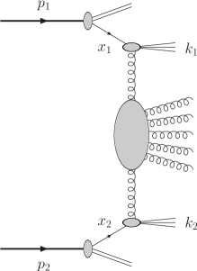
Figure 1: Mueller-Navelet jet production process.

where the $i,j$ indices specify the parton types (quarks $q=u,d,s,c,b$; antiquarks $\bar{q}=\bar{u},\bar{d},\bar{s},\bar{c},\bar{b}$; or gluon $g$), $f_{i}\left(x,\mu_{F}\right)$ denotes the initial proton PDFs; $x_{1,2}$ are the longitudinal fractions of the partons involved in the hard subprocess, while $x_{J_{1,2}}$ are the jet longitudinal fractions; $\mu_{F}$ is the factorization scale; $d\hat{\sigma}_{i,j}\left(x_{1}x_{2}s,\mu_{F}\right)$ is the partonic cross section for the production of jets and $x_{1}x_{2}s\equiv\hat{s}$ is the squared center-of-mass energy of the parton-parton collision subprocess (see Fig. 1).

In the BFKL approach [2], the cross section of the hard subprocess can be written as (see Ref. [14] for the details of the derivation)

$$\frac{d\sigma}{dy_{J_{1}}dy_{J_{2}}\,d|\vec{k}_{J_{1}}|\,d|\vec{k}_{J_{2}}|d\phi_{J_{1}}d\phi_{J_{2}}}=\frac{1}{(2\pi)^{2}}\left[{\cal C}_{0}+\sum_{n=1}^{\infty}2\cos(n\phi)\,{\cal C}_{n}\right]\,,$$ (3)

where $\phi=\phi_{J_{1}}-\phi_{J_{2}}-\pi$ and the cross section ${\cal C}_{0}$ and the other coefficients ${\cal C}_{n}$ are given by

$${\cal C}_{n}\equiv\int_{0}^{2\pi}d\phi_{J_{1}}\int_{0}^{2\pi}d\phi_{J_{2}}\,\cos[n(\phi_{J_{1}}-\phi_{J_{2}}-\pi)]\,\frac{d\sigma}{dy_{J_{1}}dy_{J_{2}}\,d|\vec{k}_{J_{1}}|\,d|\vec{k}_{J_{2}}|d\phi_{J_{1}}d\phi_{J_{2}}}\;$$ (4)

$$=\frac{x_{J_{1}}x_{J_{2}}}{|\vec{k}_{J_{1}}||\vec{k}_{J_{2}}|}\int_{-\infty}^{+\infty}d\nu\,\left(\frac{x_{J_{1}}x_{J_{2}}s}{s_{0}}\right)^{\bar{\alpha}_{s}(\mu_{R})\chi(n,\nu)}$$

$$\times\alpha_{s}^{2}(\mu_{R})c_{1}(n,\nu,|\vec{k}_{J_{1}}|,x_{J_{1}})c_{2}(n,\nu,|\vec{k}_{J_{2}}|,x_{J_{2}})\,$$

$$\times\left[1+\alpha_{s}(\mu_{R})\left(\frac{c_{1}^{(1)}(n,\nu,|\vec{k}_{J_{1}}|,x_{J_{1}})}{c_{1}(n,\nu,|\vec{k}_{J_{1}}|,x_{J_{1}})}+\frac{c_{2}^{(1)}(n,\nu,|\vec{k}_{J_{2}}|,x_{J_{2}})}{c_{2}(n,\nu,|\vec{k}_{J_{2}}|,x_{J_{2}})}\right)\right.$$

$$\left.+\bar{\alpha}_{s}^{2}(\mu_{R})\ln\left(\frac{x_{J_{1}}x_{J_{2}}s}{s_{0}}\right)\left(\bar{\chi}(n,\nu)+\frac{\beta_{0}}{8C_{A}}\chi(n,\nu)\left(-\chi(n,\nu)+\frac{10}{3}+\ln\frac{\mu_{R}^{4}}{\vec{k}_{J_{1}}^{2}\vec{k}_{J_{2}}^{2}}\right)\right)\right]\;.$$

Here $\bar{\alpha}_{s}(\mu_{R})\equiv\alpha_{s}(\mu_{R})N_{c}/\pi$, with $N_{c}$ the number of colors,

$$\beta_{0}=\frac{11}{3}N_{c}-\frac{2}{3}n_{f}$$ (5)

is the first coefficient of the QCD $\beta$-function,

$$\chi\left(n,\nu\right)=2\psi\left(1\right)-\psi\left(\frac{n}{2}+\frac{1}{2}+i\nu\right)-\psi\left(\frac{n}{2}+\frac{1}{2}-i\nu\right)$$ (6)

is the LO BFKL characteristic function,

$$c_{1}(n,\nu,|\vec{k}|,x)=2\sqrt{\frac{C_{F}}{C_{A}}}(\vec{k}^{\,2})^{i\nu-1/2}\,\left(\frac{C_{A}}{C_{F}}f_{g}(x,\mu_{F})+\sum_{a=q,\bar{q}}f_{q}(x,\mu_{F})\right)$$ (7)

and

$$c_{2}(n,\nu,|\vec{k}|,x)=\biggl{[}c_{1}(n,\nu,|\vec{k}|,x)\biggr{]}^{*}\;,$$ (8)

are the LO jet vertices in the $\nu$-representation. The remaining objects are related with the NLO corrections of the BFKL kernel ($\bar{\chi}(n,\nu)$) and of the jet vertices in the small-cone approximation ($c_{1,2}^{(1)}(n,\nu,|\vec{k}_{J_{2}}|,x_{J_{2}})$) in the $\nu$-representation. Their expressions are given in Eqs. (23), (36) and (37) of Ref. [14].

The representation (4) is valid both in the leading logarithm approximation (LLA), which means resummation of leading energy logarithms, all terms $\left(\alpha_{s}\ln\left(s\right)\right)^{n}$, and in the next-to-leading approximation (NLA), which means resummation of all terms $\alpha_{s}\left(\alpha_{s}\ln\left(s\right)\right)^{n}$. The scale $s_{0}$ is artificial. It is introduced in the BFKL approach at the time to perform the Mellin transform from the $s$-space to the complex angular momentum plane and cancels in the full expression, up to terms beyond the NLA.

Eq. (4) represents just one of infinitely many representations of the coefficients ${\cal C}_{n}$. One can consider alternative representations, aiming at catching some of the unknown next-to-NLA corrections. Introducing for the sake of brevity the definitions

$$Y=\ln\frac{x_{J_{1}}x_{J_{2}}s}{|\vec{k}_{J_{1}}||\vec{k}_{J_{2}}|}\;,\;\;\;\;\;Y_{0}=\ln\frac{s_{0}}{|\vec{k}_{J_{1}}||\vec{k}_{J_{2}}|}\;,$$

the representations we will use in this work are the following:

• the so-called exponentiated representation,

  $${\cal C}_{n}^{\rm exp} = \frac{x_{J_{1}}x_{J_{2}}}{|\vec{k}_{J_{1}}||\vec{k}_{J_{2}}|}\int_{-\infty}^{+\infty}d\nu\ e^{(Y-Y_{0})\bigl{[}\bar{\alpha}_{s}\left(\mu_{R}\right)\chi\left(n,\nu\right)+\bar{\alpha}_{s}^{2}\left(\mu_{R}\right)\left(\chi^{\left(1\right)}\left(n,\nu\right)+\frac{\beta_{0}}{8C_{A}}\chi\left(n,\nu\right)\log\frac{\mu_{R}^{4}}{\vec{k}_{J_{1}}^{2}\vec{k}_{J_{2}}^{2}}\right)\bigr{]}}\alpha_{s}^{2}\left(\mu_{R}\right)$$ (9)

  $$\times c_{1}\left(n,\nu\right)c_{2}\left(n,\nu\right)\left[1+\alpha_{s}\left(\mu_{R}\right)\left(\frac{c_{1}^{\left(1\right)}\left(n,\nu\right)}{c_{1}\left(n,\nu\right)}+\frac{c_{2}^{\left(1\right)}\left(n,\nu\right)}{c_{2}\left(n,\nu\right)}\right)\right]\;,$$

  where the dependence on $|\vec{k}_{J_{i}}|$ and $x_{J_{i}}$ in $c_{1,2}^{(1)}$ has been omitted for simplicity and

  $$\chi^{\left(1\right)}\left(n,\nu\right)=\bar{\chi}\left(n,\nu\right)+\frac{\beta_{0}}{8C_{A}}\chi\left(n,\nu\right)\left(-\chi\left(n,\nu\right)+\frac{10}{3}\right)\;,$$

  with $\bar{\chi}(n,\nu)$ given by Eq. (23) in Ref. [14].

• the exponentiated representation with an extra, irrelevant in the NLA term, given by the product of the NLO corrections of the two jet vertices,

  $${\cal C}_{n}^{\rm sq} = \frac{x_{J_{1}}x_{J_{2}}}{|\vec{k}_{J_{1}}||\vec{k}_{J_{2}}|}\int_{-\infty}^{+\infty}d\nu\ e^{(Y-Y_{0})\bigl{[}\bar{\alpha}_{s}\left(\mu_{R}\right)\chi\left(n,\nu\right)+\bar{\alpha}_{s}^{2}\left(\mu_{R}\right)\left(\chi^{\left(1\right)}\left(n,\nu\right)+\frac{\beta_{0}}{8C_{A}}\chi\left(n,\nu\right)\log\frac{\mu_{R}^{4}}{\vec{k}_{J_{1}}^{2}\vec{k}_{J_{2}}^{2}}\right)\bigr{]}}\alpha_{s}^{2}\left(\mu_{R}\right)$$ (10)

  $$\times c_{1}\left(n,\nu\right)c_{2}\left(n,\nu\right)\left[1+\alpha_{s}\left(\mu_{R}\right)\left(\frac{c_{1}^{\left(1\right)}\left(n,\nu\right)}{c_{1}\left(n,\nu\right)}+\frac{c_{2}^{\left(1\right)}\left(n,\nu\right)}{c_{2}\left(n,\nu\right)}\right)\right.$$

  $$+ \left.\alpha_{s}^{2}\left(\mu_{R}\right)\left(\frac{c_{1}^{\left(1\right)}\left(n,\nu\right)}{c_{1}\left(n,\nu\right)}\frac{c_{2}^{\left(1\right)}\left(n,\nu\right)}{c_{2}\left(n,\nu\right)}\right)\right]\;,$$

• the exponentiated representation with an RG-improved kernel,

  $${\cal C}_{n}^{\rm RG} = \frac{x_{J_{1}}x_{J_{2}}}{|\vec{k}_{J_{1}}||\vec{k}_{J_{2}}|}\int_{-\infty}^{+\infty}d\nu\ e^{(Y-Y_{0})\bigl{[}\bar{\alpha}_{s}\left(\mu_{R}\right)\chi\left(n,\nu\right)+\bar{\alpha}_{s}^{2}\left(\mu_{R}\right)\left(\chi^{\left(1\right)}\left(n,\nu\right)+\frac{\beta_{0}}{8C_{A}}\chi\left(n,\nu\right)\log\frac{\mu_{R}^{4}}{\vec{k}_{J_{1}}^{2}\vec{k}_{J_{2}}^{2}}\right)+\chi_{RG}\left(n,\nu\right)\bigr{]}}$$ (11)

  $$\times \alpha_{s}^{2}\left(\mu_{R}\right)c_{1}\left(n,\nu\right)c_{2}\left(n,\nu\right)\left[1+\alpha_{s}\left(\mu_{R}\right)\left(\frac{c_{1}^{\left(1\right)}\left(n,\nu\right)}{c_{1}\left(n,\nu\right)}+\frac{c_{2}^{\left(1\right)}\left(n,\nu\right)}{c_{2}\left(n,\nu\right)}\right)\right]\;,$$

  where $\chi^{(1)}_{\rm RG}(n,\nu)$ is given in Eqs. (13)-(15) of Ref. [15];

• a combination of the previous two representations,

  $${\cal C}_{n}^{\rm RG+sq} = \int_{-\infty}^{+\infty}d\nu\ e^{(Y-Y_{0})\bigl{[}\bar{\alpha}_{s}\left(\mu_{R}\right)\chi\left(n,\nu\right)+\bar{\alpha}_{s}^{2}\left(\mu_{R}\right)\left(\chi^{\left(1\right)}\left(n,\nu\right)+\frac{\beta_{0}}{8C_{A}}\chi\left(n,\nu\right)\log\frac{\mu_{R}^{4}}{\vec{k}_{J_{1}}^{2}\vec{k}_{J_{2}}^{2}}\right)+\chi_{RG}\left(n,\nu\right)\bigr{]}}$$ (12)

  $$\times \frac{x_{J_{1}}x_{J_{2}}}{|\vec{k}_{J_{1}}||\vec{k}_{J_{2}}|}\alpha_{s}^{2}\left(\mu_{R}\right)c_{1}\left(n,\nu\right)c_{2}\left(n,\nu\right)\left[1+\alpha_{s}\left(\mu_{R}\right)\left(\frac{c_{1}^{\left(1\right)}\left(n,\nu\right)}{c_{1}\left(n,\nu\right)}+\frac{c_{2}^{\left(1\right)}\left(n,\nu\right)}{c_{2}\left(n,\nu\right)}\right)\right.$$

  $$+ \left.\alpha_{s}^{2}\left(\mu_{R}\right)\left(\frac{c_{1}^{\left(1\right)}\left(n,\nu\right)}{c_{1}\left(n,\nu\right)}\frac{c_{2}^{\left(1\right)}\left(n,\nu\right)}{c_{2}\left(n,\nu\right)}\right)\right]\;.$$

3 Numerical results

In this Section we present our results for the dependence on $Y=y_{J_{1}}-y_{J_{2}}$ of the coefficients ${\cal C}_{n}$ and of their ratios ${\cal R}_{nm}\equiv{\cal C}_{n}/{\cal C}_{m}$. Among them, the ratios of the form $R_{n0}$ have a simple physical interpretation, being the azimuthal correlations $\langle\cos(n\phi)\rangle$.

In order to match the kinematical cuts used by the CMS collaboration, we will consider the integrated coefficients given by

$$C_{n}=\int_{y_{1,\rm min}}^{y_{1,\rm max}}dy_{1}\int_{y_{2,\rm min}}^{y_{2,\rm max}}dy_{2}\int_{k_{J_{1},\rm min}}^{\infty}dk_{J_{1}}\int_{k_{J_{2},\rm min}}^{\infty}dk_{J_{2}}\delta\left(y_{1}-y_{2}-Y\right){\cal C}_{n}\left(y_{J_{1}},y_{J_{2}},k_{J_{1}},k_{J_{2}}\right)\;,$$ (13)

with $y_{1,\rm min}=y_{2,\rm min}=-4.7$, $y_{1,\rm max}=y_{2,\rm max}=4.7$, $k_{J_{1},\rm min}=k_{J_{2},\rm min}=35$ GeV, and their ratios $R_{nm}\equiv C_{n}/C_{m}$. We fix the jet cone size at the value $R=0.5$ and the center-of-mass energy at $\sqrt{s}=7$ TeV. We use the PDF set MSTW2008nlo [20] and the two-loop running coupling with $\alpha_{s}\left(M_{Z}\right)=0.11707$.

As discussed in the Introduction, to improve the stability of the perturbative series, which is particularly relevant in the BFKL framework, several methods have been devised for the optimal choice of the several energy scales entering the above expressions. We will use the following:

• principle of minimal sensitivity (PMS) [10],

• fast apparent convergence (FAC) [11],

• Brodsky-LePage-McKenzie (BLM) method [12].

3.1 PMS

We used an adaptation of the standard PMS method, as usual in our works, valid when more than one energy scale is present. The optimal choices for $\mu_{R}$ and $s_{0}$ are those values for which the physical observable under exam exhibits the minimal sensitivity under variation of both these scales.

We applied the method to the four representations given in Eqs. (9)-(12). As for the optimal choice of the third scale, the factorization scale $\mu_{F}$, we considered the following two options:

(i) let $\mu_{F}$ follow the same fate of the renormalization scale $\mu_{R}$,

(ii) fix $\mu_{F}$ at $|\vec{k}_{J_{1}}|$ in the vertex of the jet 1 and at $|\vec{k}_{J_{2}}|$ in the vertex of the jet 2.

This leads to consider the eight following possibilities:

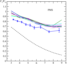
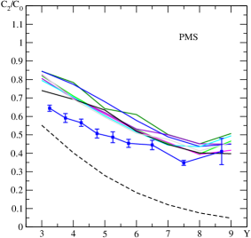
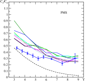
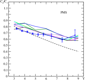
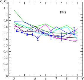
Figure 2: $Y$ dependence of several azimuthal correlations and some of their ratios. Results were obtained with the PMS method. The dashed line gives the LLA BFKL result; the colored broken lines give the NLA BFKL result for the eight options NLA_i, $i=1,...,8$ considered (see text).

NLA1,	$[{\cal C}_{n}^{\rm exp}]_{\mu_{F}=\mu_{R}}$	(Eq. (9) + option (i); dark green in Figs. 2)
NLA2,	$[{\cal C}_{n}^{\rm exp}]_{\mu_{F}=k_{J_{i}}}$	(Eq. (9) + option (ii); green in Figs. 2)
NLA3,	$[{\cal C}_{n}^{\rm sq}]_{\mu_{F}=\mu_{R}}$	(Eq. (10)+ option (i); violet in Figs. 2)
NLA4,	$[{\cal C}_{n}^{\rm sq}]_{\mu_{F}=k_{J_{i}}}$	(Eq. (10) + option (ii); magenta in Figs. 2)
NLA5,	$[{\cal C}_{n}^{\rm RG}]_{\mu_{F}=\mu_{R}}$	(Eq. (11) + option (i); blue in Figs. 2)
NLA6,	$[{\cal C}_{n}^{\rm RG}]_{\mu_{F}=k_{J_{i}}}$	(Eq. (11)+ option (ii); cyan in Figs. 2)
NLA7,	$[{\cal C}_{n}^{\rm RG+sq}]_{\mu_{F}=\mu_{R}}$	(Eq. (12) + option (i); black in Figs. 2)
NLA8,	$[{\cal C}_{n}^{\rm RG+sq}]_{\mu_{F}=k_{J_{i}}}$	(Eq. (12) + option (ii); gray in Figs. 2)

Following Refs. [6, 14, 15], in our search of the optimal values for the $Y_{0}$ and $\mu_{R}$, we considered integer values for $Y_{0}$ in the range $0\div 6$ and values for $\mu_{R}$ given by multiples of $\sqrt{|\vec{k}_{J_{1}}||\vec{k}_{J_{2}}|}$,

$$\mu_{R}=n_{R}\sqrt{|\vec{k}_{J_{1}}||\vec{k}_{J_{2}}|}\;,$$ (14)

with the integer $n_{R}$ in the range $1\div 9$.

We looked for stationary points of the coefficient $C_{n}$ in the $Y_{0}-n_{R}$ plane, then the ratios $C_{n}/C_{m}$ were obtained indirectly by using the optimal results for the coefficients $C_{n}$ and $C_{m}$. In particular, following Ref. [16], we studied the ratios $R_{10}$, $R_{20}$, $R_{30}$, $R_{21}$ and $R_{32}$. We carried out this analysis for all the representations NLA_i, $i$=1,…,8, listed above. Results are reported in Tables 1-5 and in Figs. 2. For the sake of brevity, we do not show in these Tables the optimal values of $Y_{0}-n_{R}$, but simply say that they are quite sparse in the given intervals, with more recurrent values for $Y_{0}$ in the range $2\div 5$ and for $n_{R}$ in the range $2\div 6$.

We can see that the theoretical predictions overshoot data at all values of $Y$ in the cases of $C_{1}/C_{0}$ and $C_{2}/C_{0}$ and at the smaller $Y$’s for $C_{3}/C_{0}$, while there is a agreement, at least for some of the eight options, for the ratios $C_{2}/C_{1}$ and $C_{3}/C_{2}$.

3.2 FAC

This method consists in fixing the renormalization scale $\mu_{R}$ at the value for which the highest-order correction term is exactly zero. In our case, the application of this method requires an adaptation, since there is a second energy parameter to take care of, $Y_{0}$.

We applied it to the representation labeled by NLA₁ and, for each $Y_{0}$ in a finite set of integer and half-integer values in the range 0-6, we found the value of $\mu_{R}$ such that the highest-order correction term of a certain coefficient $C_{n}$ is exactly zero. Then, a stationary point was searched for varying $Y_{0}$ in the given set.

This method in general did not allow to find clear regions of stability. Nevertheless, we report some of our results in Table 6, for the sake of comparison with the other methods.

3.3 BLM

This method consists in choosing the scale $\mu_{R}$ such that it makes vanish completely the $\beta_{0}$-dependence of a given observable.

Also in this case we considered only the representation labeled by NLA₁, i.e. the exponential representation with $\mu_{F}=\mu_{R}$. We implemented the BLM procedure in a slightly different way from Ref. [18]. As a matter of fact, we realized that a clear-cut way to implement this procedure in the present case is not obviously found. We rather implemented two variants of the BLM method, dubbed $(a)$ and $(b)$, and give here all the relevant formulae, but refer to a separate publication for details [21].

The variant $(a)$ is given by

$${\cal C}_{n}^{\rm exp-BLM_{a}} = \frac{x_{J_{1}}x_{J_{2}}}{|\vec{k}_{J_{1}}||\vec{k}_{J_{2}}|}\int_{-\infty}^{+\infty}d\nu\ e^{(Y-Y_{0})\left[\bar{\alpha}_{s}\left(\mu_{R}\right)\chi\left(n,\nu\right)+\bar{\alpha}_{s}^{2}\left(\mu_{R}\right)\left(\bar{\chi}\left(n,\nu\right)-\frac{T^{\beta}}{C_{A}}\chi\left(n,\nu\right)-\frac{\beta_{0}}{8C_{A}}\chi^{2}\left(n,\nu\right)\right)\right]}\alpha_{s}^{2}\left(\mu_{R}\right)$$ (15)

$$\times c_{1}\left(n,\nu\right)c_{2}\left(n,\nu\right)\left[1-\frac{2}{\pi}\alpha_{s}\left(\mu_{R}\right)T^{\beta}+\alpha_{s}\left(\mu_{R}\right)\left(\frac{\bar{c}_{1}^{\left(1\right)}\left(n,\nu\right)}{c_{1}\left(n,\nu\right)}+\frac{\bar{c}_{2}^{\left(1\right)}\left(n,\nu\right)}{c_{2}\left(n,\nu\right)}\right)\right]\;,$$

with $\mu_{R}$ fixed at the value

$$(\mu_{R}^{\rm BLM})^{2}=k_{J_{1}}k_{J_{2}}\ \exp\left[2\left(1+\frac{2}{3}I\right)-\frac{5}{3}\right]\;;$$ (16)

the variant $(b)$ is given by

$${\cal C}_{n}^{\rm exp\ BLM_{b}} = \frac{x_{J_{1}}x_{J_{2}}}{|\vec{k}_{J_{1}}||\vec{k}_{J_{2}}|}\int_{-\infty}^{+\infty}d\nu\ e^{(Y-Y_{0})\left[\bar{\alpha}_{s}\left(\mu_{R}\right)\chi\left(n,\nu\right)+\bar{\alpha}_{s}^{2}\left(\mu_{R}\right)\left(\bar{\chi}\left(n,\nu\right)-\frac{T^{\beta}}{C_{A}}\chi\left(n,\nu\right)\right)\right]}\alpha_{s}^{2}\left(\mu_{R}\right)$$

$$\times c_{1}\left(n,\nu\right)c_{2}\left(n,\nu\right)$$

$$\times \left[1+\alpha_{s}\left(\mu_{R}\right)\left(\frac{\beta_{0}}{4\pi}\chi\left(n,\nu\right)-2\frac{T^{\beta}}{\pi}\right)+\alpha_{s}\left(\mu_{R}\right)\left(\frac{\bar{c}_{1}^{\left(1\right)}\left(n,\nu\right)}{c_{1}\left(n,\nu\right)}+\frac{\bar{c}_{2}^{\left(1\right)}\left(n,\nu\right)}{c_{2}\left(n,\nu\right)}\right)\right]\;,$$

with $\mu_{R}$ fixed at the value

$$(\mu_{R}^{\rm BLM})^{2}=k_{J_{1}}k_{J_{2}}\ \exp\left[2\left(1+\frac{2}{3}I\right)-\frac{5}{3}+\frac{1}{2}\chi\left(\nu,n\right)\right]\;.$$ (18)

In Eqs. (15) and (3.3), we have

$$T = T^{\beta}+T^{conf}\;,$$

$$T^{\beta} = -\frac{\beta_{0}}{2}\left(1+\frac{2}{3}I\right)\;,$$

$$T^{conf} = \frac{C_{A}}{8}\left[\frac{17}{2}I+\frac{3}{2}\left(I-1\right)\xi+\left(1-\frac{1}{3}I\right)\xi^{2}-\frac{1}{6}\xi^{3}\right]\;,$$

where $I=-2\int_{0}^{1}dx\frac{\ln\left(x\right)}{x^{2}-x+1}\simeq 2.3439$ and $\xi$ is a gauge parameter, fixed at zero, while $\bar{c}_{i}^{(1)}/c_{i}$ is the NLO impact factor defined as in Eqs. (9)-(12) with the terms proportional to $\beta_{0}$ removed.

Results are reported in Tables 7 and 8 and in Figs. 3. We can see that, except for the ratio $C_{1}/C_{0}$, the agreement with experimental data is very good, for both variants, at the larger values of $Y$.

4 Discussion

In this paper we have studied several, equivalent within the NLA, representations of the coefficients entering the definition of cross section, azimuthal decorrelations and ratios of azimuthal decorrelations, and have compared them with the corresponding CMS experimental data at the center-of-mass energy of 7 TeV.

We have considered three different procedures to optimize the perturbative series (PMS, FAC and BLM, the latter in two variants) and found that:

• the FAC method does not lead to any sensible result for most observables;

• the ratios $C_{2}/C_{1}$ and $C_{3}/C_{2}$ are quite well reproduced basically by all representations treated with the PMS method;

• the BLM method, implemented in the exponentiated representation, reproduces quite well all the ratios studied in this work, in the region $Y\gtrsim 6$; we see, however, a sizeable difference in the theoretical prediction of the value of $C_{0}$ between the two variants $(a)$ and $(b)$; also in Ref. [18] an important effect on the cross section is reported when the BLM method is implemented together with an RG-improved kernel, than with the standard non-RG-improved kernel.

We believe that the information we gathered in this work can be of help in preparing new predictions for the same observables considered the increased collision energy of LHC after the LS1. In particular, it could be useful for estimates of theoretical uncertainties. Our numerical analysis shows that these uncertainties are rather large, in general due to very large NLA BFKL corrections in the considered kinematical range. In particular, the plots in Fig. 2 demonstrate that, within the PMS method, results obtained using different representations of the NLA BFKL amplitude are quite different one from the other. We stress that this type of uncertainty is often not considered and in the NLA BFKL analysis one uses just some prescribed representation of NLA BFKL amplitude. We believe that one should be aware of this “representation” uncertainty, until the time will come when some deeper insight into the physics of effects beyond NLA BFKL will allow to choose a definite representation of NLA BFKL amplitude. Perhaps, the BLM optimization procedure gives us a hint towards the right direction, because theoretical predictions derived with BLM [18] turned to be in a rather good agreement with CMS data. Our own BLM calculations presented in Fig. 3 support this statement, though, comparing our results with the plots of Ref. [18], we see that our predictions lies somewhat beyond the range of the theoretical uncertainty bound accepted there. Most probably this difference is related with the above mentioned “representation uncertainty”, indeed our BLM amplitudes in Eqs. (15) and (3.3), in contrast with [18], do not include the product of the two NLO impact factors terms.

Meanwhile, it would be also useful to address, on the experimental side, some possible issues which could be sources of mismatch with the way in which Mueller-Navelet jets are defined in theory and that are not easy to be revealed in the comparison with theoretical predictions, for being the latter affected in their turn by systematic effects of the same amount. We list below a few of them.

• In data analysis defining the $Y$ value for a given final state with two jets, the rapidity of one of the two jets could be so small, say $|y_{J_{i}}|\lesssim 2$, that this jet is actually produced in the central region, rather than in one of the two forward regions. The longitudinal momentum fractions of the parent partons that generate a central jet are very small, and one can naturally expect sizable corrections to the vertex of this jet, due to the fact that the collinear factorization approach used in the derivation of the result for jet vertex is not designed for the region of small $x$. We believe that a combined theoretical approach that uses collinear factorization for the forward and $k_{t}$-factorization for the central jets should be more relevant in such kinematics.

• The other issue is related with the experimental event selection for Mueller-Navelet jet analysis in a situation when more that two jets are detected in one single event. In particular, let us consider events with three jets in the final state, two of them being forward in one direction (with large positive rapidities, say, $y_{1}$ and $y_{2}$ with $y_{1}>y_{2}$), and the third being forward in the other direction (with large negative rapidity, say, $y_{3}$). Traditionally, as in the current CMS analysis, such event is selected as a single Mueller-Navelet jet, where the two selected Mueller-Navelet jets are those having the largest interval in rapidity. In our example, these are the jets with rapidities $y_{1}$ and $y_{3}$, so that $Y=y_{1}-y_{3}$. This selection method is convenient for the experimental analysis, but it does not match the definition of Mueller-Navelet jets in the theoretical NLA BFKL calculations. Examining the derivation of the NLA jet vertex [7], one can see that what is calculated in the theory is an inclusive jet production in the forward region, with some prescribed values of rapidity and transverse momentum $\vec{k}$, where possible additional parton radiation is attributed to the inclusive hadron system $X$. Returning to our example of event with three detected jets, we see that in order to match the theory it should lead to the selection of two separate Mueller-Navelet jets events (i.e. it should be counted twice): a pair of Mueller-Navelet jets with rapidities $y_{1}$ and $y_{3}$ (then $Y=y_{1}-y_{3}$) and another pair of Mueller-Navelet jets with rapidities $y_{2}$ and $y_{3}$ (then $Y=y_{2}-y_{3}$). This mismatch between experimental event selection and theory appears in NLA BFKL and could be important due to very large value of NLA BFKL corrections. The issue may be clarified either from the experimental side, changing the Mueller-Navelet jet selection criterion, or from the theoretical side, which could require the generation of separate jet events with Monte Carlo methods.

• The use of symmetric cuts in the values of $k_{J_{i},\rm min}$ maximizes the contribution of the Born term in $C_{0}$, which is present for back-to-back jets only and is expected to be large, therefore making less visible the effect of the BFKL resummation in all observables involving $C_{0}$. The use of asymmetric cuts can reduce the contribution of the Born term and enhance effects with additional undetected hard gluon radiation, which makes the visibility of BFKL effect more clear in comparison to the descriptions based on fixed order DGLAP approach.

• The experimental determination of the Mueller-Navelet total cross section, $C_{0}$, would provide for a yardstick which could help choosing a definite NLA representation.

Table 1: $C_{1}/C_{0}$ in the LLA and in the NLA according to the eight different representations discussed in the text; results obtained with the PMS method.

$Y$	LLA	NLA1	NLA2	NLA3	NLA4	NLA5	NLA6	NLA7	NLA8
3	0.6845	1.0099	0.9261	0.9762	0.9558	1.0129	0.8970	0.9756	0.9642
4	0.5544	0.9112	0.8772	0.8891	0.8915	0.9052	0.8962	0.8721	0.8811
5	0.4273	0.8563	0.8332	0.8564	0.8477	0.8433	0.8183	0.8609	0.8207
6	0.3195	0.7972	0.7837	0.7799	0.7802	0.7497	0.7637	0.7736	0.7589
7	0.2342	0.7248	0.7291	0.7433	0.7224	0.7060	0.7185	0.7226	0.7037
8	0.1679	0.7205	0.6889	0.7169	0.6803	0.6951	0.7281	0.6911	0.6508
9	0.1192	0.8292	0.7023	0.7262	0.6889	0.7066	0.7596	0.6894	0.7581

Table 2: $C_{2}/C_{0}$ in the LLA and in the NLA according to the eight different representations discussed in the text; results obtained with the PMS method.

$Y$	LLA	NLA1	NLA2	NLA3	NLA4	NLA5	NLA6	NLA7	NLA8
3	0.5519	0.8448	0.8205	0.8059	0.8262	0.8454	0.7949	0.7402	0.8301
4	0.4024	0.7838	0.7107	0.6974	0.6997	0.7738	0.7045	0.6924	0.6932
5	0.2791	0.6418	0.6130	0.6207	0.6132	0.6794	0.6028	0.6343	0.5956
6	0.1864	0.6100	0.5287	0.5316	0.5233	0.5781	0.5154	0.5191	0.5080
7	0.1207	0.5014	0.4536	0.4999	0.4584	0.4890	0.4440	0.4475	0.4758
8	0.0762	0.4509	0.3966	0.4514	0.3932	0.4372	0.4353	0.4017	0.4130
9	0.0479	0.5071	0.4665	0.4489	0.4164	0.4503	0.4942	0.3974	0.4572

Table 3: $C_{3}/C_{0}$ in the LLA and in the NLA according to the eight different representations discussed in the text; results obtained with the PMS method.

$Y$	LLA	NLA1	NLA2	NLA3	NLA4	NLA5	NLA6	NLA7	NLA8
3	0.4667	0.9030	0.7143	0.6218	0.6686	0.7447	0.6920	0.6180	0.6891
4	0.3199	0.6816	0.5534	0.5021	0.5424	0.6785	0.5737	0.4944	0.5373
5	0.2075	0.5178	0.4907	0.4494	0.4391	0.5258	0.4279	0.5121	0.4286
6	0.1281	0.4428	0.4481	0.3577	0.4401	0.3874	0.3403	0.3443	0.3422
7	0.0767	0.3497	0.3430	0.3071	0.2810	0.3912	0.3320	0.2966	0.2819
8	0.0451	0.3107	0.3260	0.2658	0.2378	0.3073	0.3466	0.2526	0.2833
9	0.0264	0.3475	0.3289	0.2605	0.3217	0.2977	0.2951	0.2470	0.3414

Table 4: $C_{2}/C_{1}$ in the LLA and in the NLA according to the eight different representations discussed in the text; results obtained with the PMS method.

$Y$	LLA	NLA1	NLA2	NLA3	NLA4	NLA5	NLA6	NLA7	NLA8
3	0.8063	0.8366	0.8859	0.8256	0.8644	0.8346	0.8862	0.7588	0.8610
4	0.7258	0.8602	0.8102	0.7844	0.7849	0.8549	0.7861	0.7939	0.7868
5	0.6531	0.7494	0.7357	0.7247	0.7234	0.8055	0.7366	0.7368	0.7257
6	0.5835	0.7651	0.6746	0.6815	0.6707	0.7710	0.6749	0.6711	0.6693
7	0.5154	0.6917	0.6221	0.6725	0.6346	0.6926	0.6180	0.6193	0.6762
8	0.4541	0.6258	0.5757	0.6296	0.5780	0.6290	0.5979	0.5813	0.6346
9	0.4015	0.6115	0.6643	0.6181	0.6044	0.6373	0.6506	0.5765	0.6031

Table 5: $C_{3}/C_{2}$ in the LLA and in the NLA according to the eight different representations discussed in the text; results obtained with the PMS method.

$Y$	LLA	NLA1	NLA2	NLA3	NLA4	NLA5	NLA6	NLA7	NLA8
3	0.8456	1.0689	0.8705	0.7716	0.8092	0.8808	0.8706	0.8349	0.8301
4	0.7951	0.8696	0.7786	0.7199	0.7752	0.8768	0.8143	0.7141	0.7750
5	0.7437	0.8068	0.8006	0.7240	0.7161	0.7740	0.7098	0.8073	0.7196
6	0.6871	0.7260	0.8477	0.6729	0.8411	0.6702	0.6602	0.6633	0.6736
7	0.6355	0.6975	0.7563	0.6144	0.6130	0.7999	0.7477	0.6629	0.5924
8	0.5910	0.6892	0.8221	0.5889	0.6048	0.7030	0.7961	0.6287	0.6859
9	0.5513	0.6853	0.7050	0.5803	0.7726	0.6611	0.5971	0.6213	0.7467

Table 6: $C_{0}$, $C_{1}$ and $C_{1}/C_{0}$ in the representation NLA₁ with the FAC method; columns three, four, six and seven give the optimal values for $Y_{0}$ and $\mu_{R}/\sqrt{|\vec{k}_{J_{1}}||\vec{k}_{J_{2}}|}$.

$Y$	$C_{0}$ [nb]	$Y_{0}$	$n_{R}$	$C_{1}$ [nb]	$Y_{0}$	$n_{R}$	$C_{1}/C_{0}$
3	2584.9	2	3.1	–	–	–	–
4	928.303	2	2.7	–	–	–	–
5	291.053	3	2.9	249.865	3	2.9	0.8585
6	75.0725	3	2.7	60.1738	3	2.3	0.8015
7	13.8129	3.5	2.9	10.5419	3	1.9	0.7632
8	1.23915	4	3.3	0.918584	3	1.9	0.7413
9	0.0135918	5	4.7	0.00993695	4	3.1	0.7311

Table 7: $C_{0}$, $C_{1}$, $C_{2}$ and $C_{3}$ in the representation NLA₁ with the BLM method, in both variants $(a)$ and $(b)$.

	$C_{0}$ [nb]		$C_{1}$ [nb]		$C_{2}$ [nb]		$C_{3}$ [nb]
$Y$	$(a)$	$(b)$	$(a)$	$(b)$	$(a)$	$(b)$	$(a)$	$(b)$
3	2240.88	2267.12	2150.07	2180.83	1834.76	1860.73	1539.24	1578.51
4	794.934	814.956	707.761	726.72	543.584	567.018	433.784	451.898
5	237.577	252.277	198.863	206.239	138.340	146.97	101.337	109.352
6	61.6366	64.3728	45.8401	47.901	28.7511	31.1006	19.7234	21.5774
7	11.1072	11.7626	7.60735	7.99795	4.3031	4.73926	2.73730	3.0664
8	0.96651	1.05596	0.63085	0.67637	0.32757	0.36776	0.19508	0.22453
9	0.00911	0.01119	0.00693	0.00742	0.00334	0.00385	0.00188	0.00224

Table 8: $C_{1}/C_{0}$, $C_{2}/C_{0}$, $C_{3}/C_{0}$, $C_{2}/C_{1}$, $C_{3}/C_{2}$ in the representation NLA₁ with the BLM method, in both variants $(a)$ and $(b)$.

	$C_{1}/C_{0}$		$C_{2}/C_{0}$		$C_{3}/C_{0}$		$C_{2}/C_{1}$		$C_{3}/C_{2}$
$Y$	$(a)$	$(b)$	$(a)$	$(b)$	$(a)$	$(b)$	$(a)$	$(b)$	$(a)$	$(b)$
3	0.9595	0.9619	0.8188	0.8207	0.6869	0.6963	0.8533	0.8532	0.8389	0.8483
4	0.8903	0.8917	0.6838	0.6958	0.5457	0.5545	0.7680	0.7802	0.7980	0.7970
5	0.8370	0.8175	0.5823	0.5826	0.4265	0.4335	0.6957	0.7126	0.7325	0.7440
6	0.7437	0.7441	0.4465	0.4831	0.3200	0.3352	0.6272	0.6493	0.6860	0.6938
7	0.6849	0.6799	0.3874	0.4029	0.2464	0.2607	0.5657	0.5926	0.6361	0.6470
8	0.6602	0.6405	0.3389	0.3483	0.2018	0.2126	0.5134	0.5437	0.5955	0.6105
9	0.7604	0.6634	0.3670	0.3441	0.2065	0.2005	0.4826	0.5187	0.5627	0.5826

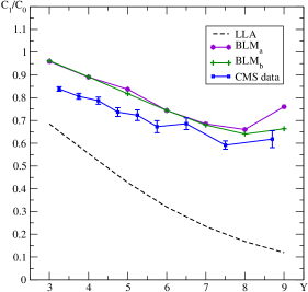
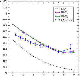
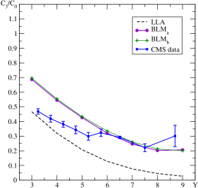
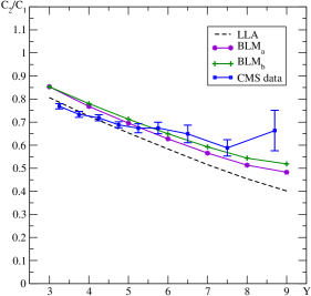
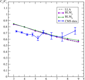
Figure 3: $Y$ dependence of several azimuthal correlations and some of their ratios. Results were obtained with the two variants of the BLM method. The dashed line gives the LLA BFKL result.

Acknowledgments

D.I. thanks the Dipartimento di Fisica dell’Università della Calabria and the Istituto Nazionale di Fisica Nucleare (INFN), Gruppo collegato di Cosenza, for warm hospitality and financial support. The work of D.I. was also supported in part by the grant RFBR-13-02-00695-a.
F.C. and B.M thank A. Sabio Vera for fruitful discussions and the Instituto de Física Teórica/UAM-CSIC, for warm hospitality during the early stages of this work.
The work of B.M. was supported in part by the grant RFBR-13-02-90907 and by the European Commission, European Social Fund and Calabria Region, that disclaim any liability for the use that can be done of the information provided in this paper.
We thank F.G. Celiberto for noticing a mismatch between the content of Tables 7 and 8 of the previous version of the paper and the plots in Fig. 3 and for checking all entries in these Tables by an independent Fortran program.

References

- [1] A.H. Mueller and H. Navelet, Nucl. Phys. B282, 727 (1987).
- [2] V.S. Fadin, E.A. Kuraev, L.N. Lipatov, Phys. Lett. B60, 50 (1975); E.A. Kuraev, L.N. Lipatov and V.S. Fadin, Zh. Eksp. Teor. Fiz. 71, 840 (1976) [Sov. Phys. JETP 44, 443 (1976)]; 72, 377 (1977) [45, 199 (1977)]; Ya.Ya. Balitskii and L.N. Lipatov, Sov. J. Nucl. Phys. 28, 822 (1978).
- [3] V.N. Gribov, L.N. Lipatov, Sov. J. Nucl. Phys. 15, 438 (1972); G. Altarelli, G. Parisi, Nucl. Phys. B126, 298 (1977); Y.L. Dokshitzer, Sov. Phys. JETP 46, 641 (1977).
- [4] A. Sabio Vera and F. Schwennsen, Nucl.Phys. B 776 (2007) 170; A. Sabio Vera, Nucl.Phys. B 746 (2006) 1.
- [5] V.S. Fadin and L.N. Lipatov, Phys. Lett. B 429 (1998) 127; M. Ciafaloni and G. Camici, Phys. Lett. B 430 (1998) 349.
- [6] D.Yu. Ivanov and A. Papa, Nucl. Phys. B 732, 183 (2006); Eur. Phys. J. C 49, 947 (2007); F. Caporale, A. Papa and A. Sabio Vera, Eur. Phys. J. C 53, 525 (2008).
- [7] J. Bartels, D. Colferai and G.P. Vacca, Eur. Phys. J. C24, 83-99 (2002); Eur. Phys. J. C29, 235-249 (2003); F. Caporale, D.Yu Ivanov, B. Murdaca, A. Papa and A. Perri, JHEP 1202, 101 (2012).
- [8] D.Yu Ivanov and A. Papa, JHEP 1205, 086 (2012).
- [9] G.P. Salam, JHEP 9807 (1998) 019; M. Ciafaloni, D. Colferai, G.P. Salam, A.M. Stasto, Phys. Lett. B 587 (2004) 87; Phys. Rev. D 68 (2003) 114003; Phys. Lett. B 576 (2003) 143; Phys. Lett. B 541 (2002) 314; Phys. Rev. D 66 (2002) 054014; M. Ciafaloni, D. Colferai, G.P. Salam, JHEP 0007 (2000) 054; JHEP 9910 (1999) 017; Phys. Rev. D 60 (1999) 114036; M. Ciafaloni, D. Colferai, Phys. Lett. B 452 (1999) 372; A. Sabio Vera, Nucl. Phys. B 722 (2005) 65.
- [10] P.M. Stevenson, Phys. Lett. B100, 61 (1981); Phys. Rev. D 23, 2916 (1981).
- [11] G. Grunberg, Phys. Lett. B95, 70 (1980) [Erratum-ibid. B110, 501 (1982)]; ibid. B114, 271 (1982); Phys. Rev. D29, 2315 (1984).
- [12] S.J. Brodsky, G.P. Lepage, P.B. Mackenzie, Phys. Rev. D 28, 228 (1983).
- [13] D. Colferai, F. Schwennsen, L. Szymanowski, S. Wallon, JHEP 1012, 026 (2010).
- [14] F. Caporale, D.Yu Ivanov, B. Murdaca and A. Papa, Nucl. Phys. B 877, 73 (2013).
- [15] F. Caporale, B. Murdaca, A. Sabio Vera and C. Salas, Nucl. Phys. B875, 134 (2013).
- [16] CMS Collaboration, S. Chatrchyan et al., CMS PAS FSQ-12-002.
- [17] B. Ducloué, L. Szymanowski, S. Wallon, JHEP 1305, 096 (2013).
- [18] B. Ducloué, L. Szymanowski, S. Wallon, Phys. Rev. Lett. 112, 082003 (2014).
- [19] B. Ducloué, L. Szymanowski, S. Wallon, arXiv:1407.6593 [hep-ph].
- [20] A.D. Martin, W.J. Stirling, R.S. Thorne and G. Watt, Eur. Phys. J. C 63, 189 (2009).
- [21] F. Caporale, D.Yu. Ivanov, B. Murdaca and A. Papa, in preparation.