Nonlinear growing neutrino cosmology

Abstract

The energy scale of Dark Energy, $\sim 2\times 10^{-3}$ eV, is a long way off compared to all known fundamental scales – except for the neutrino masses. If Dark Energy is dynamical and couples to neutrinos, this is no longer a coincidence. The time at which Dark Energy starts to behave as an effective cosmological constant can be linked to the time at which the cosmic neutrinos become nonrelativistic. This naturally places the onset of the Universe’s accelerated expansion in recent cosmic history, addressing the why-now problem of Dark Energy. We show that these mechanisms indeed work in the Growing Neutrino Quintessence model – even if the fully nonlinear structure formation and backreaction are taken into account, which were previously suspected of spoiling the cosmological evolution. The attractive force between neutrinos arising from their coupling to Dark Energy grows as large as $10^{6}$ times the gravitational strength. This induces very rapid dynamics of neutrino fluctuations which are nonlinear at redshift $z\approx 2$. Nevertheless, a nonlinear stabilization phenomenon ensures only mildly nonlinear oscillating neutrino overdensities with a large-scale gravitational potential substantially smaller than that of cold dark matter perturbations. Depending on model parameters, the signals of large-scale neutrino lumps may render the cosmic neutrino background observable.

I Introduction

The cosmological constant $\Lambda$ has emerged as the standard explanation for the observed accelerated expansion of the Universe Perlmutter et al. (1999); Riess et al. (1998). Together with the assumption of cold dark matter (CDM), it forms the remarkably successful concordance model $\Lambda$CDM Bartelmann (2010). The proposed alternatives to the cosmological constant are already many – more complicated and often a worse fit to observational data Copeland et al. (2006). A new model should only be added to this list if it provides theoretical advantages or phenomenological aspects that neither the cosmological constant nor its most prominent competitors can offer. Growing Neutrino Quintessence (GNQ) was proposed in this spirit Amendola et al. (2008); Wetterich (2007). It addresses both the cosmological constant problem (why is the energy density of Dark Energy so small?) and the why-now problem (why has Dark Energy just started to dominate the energy budget of the Universe?) Weinberg (1989); Carroll (2001). On the phenomenological side, it predicts a time-varying neutrino mass and the formation of large-scale neutrino overdensities that might be detectable by their gravitational potentials Mota et al. (2008).

As a quintessence model Wetterich (1988); Ratra and Peebles (1988), GNQ describes the Dark Energy by a dynamical scalar field, the cosmon $\varphi$. Analogously to the inflaton in inflationary theories of the early Universe, the cosmon can describe an accelerated expansion of the Universe at late times. The similarity of the mechanism even allows for a unified picture in which the same field is responsible for both the early and the late accelerating epochs Wetterich (2013, 2014). Quintessence models address the cosmological constant problem: the energy density of Dark Energy decays, during most of the cosmological evolution, just like that of radiation and matter. Its small size today is then simply a consequence of the large age of the Universe.

In contrast to the simplest quintessence models, GNQ includes a mechanism for a natural crossover to the accelerated phase. No fine-tuning of the self-interaction potential is needed. Instead, a coupling between the cosmon and the neutrinos affects the dynamics of Dark Energy. The event of the cosmic neutrinos becoming nonrelativistic – which, due to their small masses, happens in relatively recent cosmic history – triggers the onset of Dark Energy domination.

This requires a relatively strong coupling between the cosmon and the neutrinos, which can have a natural explanation in a particle physics setting Wetterich (2007). Such a coupling has, however, a decisive impact on the evolution of perturbations in the neutrino density. The perturbations become nonlinear even on very large scales Mota et al. (2008). Furthermore, the expansion history can be affected by a nonlinear backreaction effect Pettorino et al. (2010). These technical complications motivated a comprehensive simulation technique Ayaita et al. (2012). The technique has by now matured and allows to obtain full cosmological evolutions of the model. In the technically simpler case of a constant coupling parameter, its preliminary results already inspired a consistent physical picture and an approximation scheme for the nonlinear evolution Ayaita et al. (2013). In this work, we will turn to the more natural yet technically challenging case of a field-dependent coupling. Again, a coherent (though fundamentally different) physical picture of the cosmological evolution will emerge. Our results for the first time show the full cosmological evolution of GNQ until redshift zero.

A relation between Dark Energy (in the form of a scalar field) and the neutrino masses has earlier been studied in models of ‘mass-varying neutrinos’ (MaVaNs) Fardon et al. (2004). These models share certain features with GNQ, in particular the instability problem of neutrino perturbations Afshordi et al. (2005); Bjaelde et al. (2008); Brouzakis et al. (2008). The cosmon-neutrino coupling, once strong enough, can lead to the formation of large nonlinear neutrino lumps. These lumps would, as a backreaction effect, influence the expansion dynamics of the Universe. They could even prevent the Universe from entering a phase of accelerated expansion. For GNQ, the strong backreaction effect of stable neutrino lumps on the expansion dynamics has been shown in a simulation Ayaita et al. (2012). Our results, however, provide a counterexample in which – in spite of the instability of perturbations – the backreaction effect remains small and the expansion dynamics is affected only marginally. We anticipate this numerical result in Fig. 1.

\psfrag{xlabel}[B][c][.9][0]{scale factor $a$}\psfrag{ylabel}[B][c][.9][0]{energy fractions $\Omega_{i}$}\includegraphics[width=195.12767pt]{omegas.eps}

Figure 1: The transition to Dark Energy domination in nonlinear growing neutrino cosmology. The figure shows the energy fraction of the coupled cosmon-neutrino fluid as obtained in a nonlinear simulation (red solid) and a purely homogeneous computation (black dashed). The two lines almost coincide, demonstrating the smallness of the “backreaction”. The individual components are the cosmon (gray dotted) and the neutrinos (green dotted). The cosmological evolution of the Dark Energy fraction is compared to a cosmological constant normalized to the same present-day Dark Energy density (blue dot-dashed).

Although we will encounter sizable backreaction effects in the interaction of Dark Energy and neutrinos, the backreaction effect on the combined cosmon-neutrino fluid is hardly visible. The evolution of the energy density of this fluid is very similar to that of a cosmological constant. The main distinction is the presence of a small fraction of Early Dark Energy.

This work is organized as follows. The next section covers a brief overview of the fundamentals of the model and the most important insights into its cosmological evolution that preceded this work. Section III will explain the main ideas of the simulation method. The numerical results in Sec. IV are followed by a physical interpretation in Sec. V sketching a coherent physical picture of the evolution. The work concludes in Sec. VI.

II Growing Neutrino Quintessence

II.1 Basic concepts

In this section, we briefly collect and explain the main ingredients that make up the GNQ model. In a nutshell, these are the cosmon $\varphi$ described as a scalar field with a canonical kinetic term and a self-interaction potential $V(\varphi)$ and the neutrinos whose masses are assumed to depend on $\varphi$. The field-dependence of the neutrino mass defines an interaction between the cosmon and the neutrinos whose coupling parameter $\beta$ is a measure of how strong this field-dependence is.

Let us take the time to go through this in more detail. The Lagrangian of the cosmon alone is of standard form

$$-\mathcal{L}_{\varphi}=\frac{1}{2}\partial^{\lambda}\varphi\partial_{\lambda}\varphi+V(\varphi).$$ (1)

Here and in the following, we use the metric signature $(-,+,+,+)$ and units where the reduced Planck mass is unity, implying $8\pi G=1$. We assume an exponential potential $V(\varphi)\propto\exp(-\alpha\varphi)$ Wetterich (2008). The details of the potential do not matter as long as it gives rise to suitable scaling solutions ensuring – for a wide range of initial conditions – that Dark Energy decays just as the dominant component (radiation and later matter). In our case, the constraints on Early Dark Energy require $\alpha\gtrsim 10$ Doran et al. (2007); Reichardt et al. (2012); Pettorino et al. (2013). The scaling solution should hold as long as neutrino masses play no role.

The second ingredient is the dependence of the neutrino masses on $\varphi$ Wetterich (2007). For simplicity, we only consider the average neutrino mass $m_{\nu}$ instead of the full mass matrix $M_{\nu}$ of the three light neutrinos. A dependence $m_{\nu}=m_{\nu}(\varphi)$ occurs if a fundamental mass scale $M$ in the mechanism of neutrino mass generation depends on $\varphi$. For example, in the cascade or induced triplet mechanism Magg and Wetterich (1980); Lazarides et al. (1981); Mohapatra and Senjanovic (1981); Schechter and Valle (1980), the neutrino masses are proportional to $M_{t}^{-2}$ where $M_{t}$ denotes the mass of a heavy $\text{SU}(2)_{L}$ triplet. If $M_{t}$ depends on $\varphi$ such that it reaches a small value near $\varphi=\varphi_{\text{crit}}$, the average neutrino mass can be approximated, in the range of interest, by the ansatz

$$m_{\nu}(\varphi)=\frac{\bar{m}}{\varphi_{\text{crit}}-\varphi}$$ (2)

with a parameter $\bar{m}$ Wetterich (2007). The formal pole at $\varphi_{\text{crit}}$ is never reached by the cosmological solution and may be considered as an artifact of the approximation. Also the behavior far away from this pole is not important for our considerations as, in this case, the cosmon-neutrino coupling is negligible. We can thus employ the relation given by Eq. (2) for the full cosmological evolution.

The cosmon-neutrino coupling $\beta$ quantifies the strength of the field-dependence of $m_{\nu}$. It is defined as

$$\beta(\varphi)\equiv-\frac{\mathrm{d}\ln m_{\nu}(\varphi)}{\mathrm{d}\varphi}=-\frac{1}{\varphi_{\text{crit}}-\varphi},$$ (3)

where, in the last step, we have used the explicit dependence of Eq. (2). When $\varphi$ approaches $\varphi_{\text{crit}}$, the coupling becomes strong and successfully stops the evolution of the cosmon. However, other functional shapes for $\beta$ are possible as well. For instance, a technically simple choice is a constant coupling $\beta=\text{const.}$ implying an exponential mass dependence $m_{\nu}(\varphi)\propto\exp(-\beta\varphi)$. A growing neutrino mass requires a negative coupling parameter $\beta<0$. The coupling between the cosmon and the neutrinos manifests itself as an energy-momentum exchange between the two components. This energy-momentum transfer is proportional to the coupling parameter $\beta(\varphi)$ and reads

$$\nabla_{\lambda}T^{\mu\lambda}_{(\varphi)} =+\beta(\varphi)\,T_{(\nu)}\partial^{\mu}\varphi,$$ (4)

$$\nabla_{\lambda}T^{\mu\lambda}_{(\nu)} =-\beta(\varphi)\,T_{(\nu)}\partial^{\mu}\varphi,$$ (5)

where $T_{(\nu)}\equiv T^{\lambda}_{(\nu)\,\lambda}=-\rho_{\nu}+3p_{\nu}$ denotes the trace of the neutrino energy-momentum tensor. Quintessence couplings of this simple type are discussed in early works on coupled Dark Energy Wetterich (1995); Amendola (2000).

Inserting the cosmon’s energy-momentum tensor in Eq. (4) yields the field equation

$$\nabla^{\lambda}\nabla_{\lambda}\varphi-V_{,\varphi}(\varphi)=\beta(\varphi)\,T_{(\nu)}.$$ (6)

It shows that the cosmon-neutrino coupling becomes only effective once the right-hand side, $\beta T_{(\nu)}$, is comparable to or larger than the potential derivative $V_{,\varphi}$. As long as the neutrinos are relativistic with $w_{\nu}\approx 1/3$, the trace $T_{(\nu)}=-\rho_{\nu}(1-3w_{\nu})$ and thereby the effect of the coupling is negligible. In this sense, the neutrinos becoming nonrelativistic serves as a trigger event. On the other hand, also $\beta(\varphi)$ grows towards large negative values as $\varphi$ rolls down its potential towards $\varphi_{\text{crit}}$. This ensures that, eventually, the effect of the coupling cancels the effect of the potential derivative. In that case, the evolution of the cosmon is essentially stopped, and the Dark Energy approximately acts as a cosmological constant with vacuum energy $V(\varphi_{\text{crit}})$. We will find that $\varphi$, and therefore the neutrino masses, oscillate around a slowly increasing value.

For a neutrino particle on a classical path, the coupling implies the equation of motion Ayaita et al. (2012)

$$\frac{\mathrm{d}u^{\mu}}{\mathrm{d}\tau}+\Gamma^{\mu}_{\alpha\beta}u^{\alpha}u^{\beta}=\beta(\varphi)\,\partial^{\mu}\varphi+\beta(\varphi)\,u^{\lambda}\partial_{\lambda}\varphi\,u^{\mu},$$ (7)

where $u^{\mu}$ is the four-velocity and $\tau$ denotes the proper time. The left-hand side is simply the motion under gravity, whereas the right-hand side includes the effects of the cosmon-neutrino coupling. For the (spatial) velocities $u^{k}$, the first term, $\beta\partial^{k}\varphi$, is similar to a potential gradient in Newtonian gravity and can be interpreted as an attractive force between the neutrinos. In the limit of small velocities, it is about $2\beta^{2}$ stronger than gravity Wintergerst et al. (2010). For relativistic velocities, it becomes negligible as the other contributions grow quadratically with components of the four-velocity $u^{\mu}$. In this case, the coupling is only important in the second term on the right-hand side, which, however, cannot change the direction of motion of the particle. Thus, the cosmon-mediated attraction of neutrinos is only effective in the nonrelativistic case.

A second important ingredient is the replacement of the Hubble damping by “cosmon acceleration”. Neglecting the (spatial) gradients $\partial^{k}\varphi$ (and, similar, for the metric), Eq. (7) becomes ($u^{0}=\gamma$)

$$\frac{\mathrm{d}u^{k}}{\mathrm{d}t} =\left[\beta(\varphi)\dot{\varphi}-2H\right]\,u^{k},$$ (8)

$$\frac{\mathrm{d}\gamma}{\mathrm{d}t} =\left[\beta(\varphi)\dot{\varphi}-H\right]\,\frac{\gamma^{2}-1}{\gamma}.$$ (9)

(This is consistent with the defining relation $\gamma^{2}=1+a^{2}u^{k}u_{k}$.) For an expanding universe, the positive sign of $H$ induces a damping of all motions. We will find that the contribution $\propto\beta\dot{\varphi}$ overwhelms the Hubble damping for important periods in the formation of nonlinear neutrino structures. The acceleration of all neutrino motions for $\dot{\varphi}<0$ will play a crucial role for the dissolution of previously formed neutrino lumps.

II.2 Cosmon-neutrino structure formation for constant coupling

Understanding structure formation in GNQ is not only important to make contact with various observational constraints such as from the cosmic microwave background (CMB) or galaxy surveys. It even is a prerequisite for obtaining reliable estimates of the expansion dynamics. This is because, as we will review in this section, nonlinear perturbations in the cosmon-neutrino fluid can lead to strong backreaction effects. They alter cosmological averages of the neutrino mass and equation of state, which, in turn, influences the evolution of Dark Energy at the background level. We explain this by briefly reviewing the main steps undertaken by previous works that have shed light on the issue Brouzakis et al. (2008); Mota et al. (2008); Schrempp and Brown (2010); Wintergerst et al. (2010); Pettorino et al. (2010); Nunes et al. (2011); Baldi et al. (2011); Ayaita et al. (2012, 2013). These works focused on the constant coupling model where $\beta$ does not depend on $\varphi$. It is technically simpler and may be regarded as a useful approximation in the case where $\beta(\varphi)$ does not vary much in late cosmology. Obtaining a realistic accelerated expansion requires couplings of order $\beta\sim-10^{2}$ if the potential is exponential with $\alpha\gtrsim 10$.

The large value of the coupling implies a fast growth of linear neutrino perturbations. The transition to the nonlinear regime can be associated roughly with the moment at which the dimensionless power spectrum $\Delta_{\nu}^{2}(k)=k^{3}P_{\nu}(k)/(2\pi^{2})$ reaches order unity. In contrast to the CDM case, this transition occurs even on very large scales leading to a breakdown of linear perturbation theory Mota et al. (2008). Let $a_{\text{nl}}(k)$ denote the cosmic scale factor at which $\Delta_{\nu}^{2}(k)=1$ in linear perturbation theory. Figure 2 shows the transition to nonlinearity (in the Newtonian gauge) for $\beta=-52$, $\alpha=10$, and a relatively large present-day average neutrino mass $m_{\nu}^{0}\approx 2.3$ eV.

\psfrag{xlabel}[B][c][.9][0]{comoving scale $k$ [$h/$Mpc]}\psfrag{ylabel}[B][c][.9][0]{transitional scale factor $a_{\text{nl}}$}\includegraphics[width=195.12767pt]{anl.eps}

Figure 2: Onset of nonlinearity for neutrino fluctuations. We show the scale factor $a_{\text{nl}}$ at which different scales enter the nonlinear regime. Compare with the corresponding figure in Ref. Mota et al. (2008).

Although the details depend on the precise parameters chosen, the qualitative finding is generic and has its origin in the instability of linear perturbations (cf. Sec. II.1).

The first scales to enter the nonlinear regime are of comoving size $\lambda\sim 100h^{-1}$Mpc (cf. Fig. 2). The overdensities at this scale evolve into massive neutrino lumps that are stable for constant $\beta$. Although the picture will be different for the varying (i. e. cosmon-dependent) coupling $\beta(\varphi)$ investigated in this work, cf. Eq. (3), it is worthwhile to discuss the main effects in the technically simpler setting of a constant coupling $\beta\sim-10^{2}$. They will reappear, albeit in a weaker form, in the varying coupling model and play a role in the physical interpretation of our results.

Two properties of the lumps were identified that imply a backreaction effect altering the expansion dynamics Nunes et al. (2011). They both lead to a suppression

$$|\overline{T_{(\nu)}}|<|T_{(\nu)}^{\text{hom}}|$$ (10)

of the actually averaged trace of the neutrino energy-momentum tensor as compared to the trace obtained in a purely homogeneous computation that neglects the nonlinear perturbations. It is, however, this trace $T_{(\nu)}$ that enters the cosmon field equation, Eq. (6). The more severely the trace is suppressed, the less effective is the coupling in stopping the evolution of the cosmon.

First, during the lump formation, the neutrinos are accelerated to higher velocities. This can lead, in particular close to the lumps’ centers, to relativistic neutrino velocities. Those neutrinos no longer contribute to $\overline{T_{(\nu)}}$ as the energy-momentum tensor of relativistic particles is approximately traceless. Second, similarly to a gravitational potential well, the local cosmon perturbation $\delta\varphi$ is negative in lumps, leading to neutrino masses $m_{\nu}(\bar{\varphi}+\delta\varphi)$ that are smaller inside the lumps than expected for the cosmological average field $\bar{\varphi}$. As $T_{(\nu)}\propto m_{\nu}$, this substantially weakens the effect of the coupling as most neutrinos will be located in lumps. The effect can be physically understood as an approximate mass freezing within lumps – the nonlinear lumps approximately decouple from the background; the local value $\varphi_{l}$ of the cosmon within the lumps no longer follows the evolution of the homogeneous component $\bar{\varphi}$ Nunes et al. (2011). We illustrate this schematically in Fig. 3.

Figure 3: The local value of the cosmon effectively decouples from the background evolution leading to an approximate mass freezing within lumps. We use arbitrary units in this schematic plot, where the core of the potential well is typically of the size of several Megaparsecs and the depth of the potential well is of order $\bar{\varphi}-\varphi(0)\sim 10^{-2}$ Ayaita et al. (2012).

In this illustration, a stable lump is located at $r=0$; within some time interval $\Delta t$, the cosmon evolves by $\Delta\varphi_{l}$ within and by $\Delta\bar{\varphi}$ far outside the lump. The figure tells us that $\varphi_{l}<\bar{\varphi}$ and $\Delta\varphi_{l}<\Delta\bar{\varphi}$. Stated differently, the background component $\bar{\varphi}$ feels a smaller neutrino mass $\overline{m_{\nu}(\varphi)}<m_{\nu}(\bar{\varphi})$, which, in addition, depends more weakly on $\bar{\varphi}$ Pettorino et al. (2010). This weaker dependence can be expressed as a weaker effective coupling

$$\beta_{\text{eff}}\equiv-\frac{\mathrm{d}\ln\overline{m_{\nu}(\varphi)}}{\mathrm{d}\bar{\varphi}},\ |\beta_{\text{eff}}|<|\beta|.$$ (11)

It postpones the onset of the accelerated expansion Ayaita et al. (2012).

For constant $\beta$, a clear physical picture and a resulting approximation scheme have emerged that describe the cosmological evolution after the formation of lumps Ayaita et al. (2013). Despite relativistic neutrino velocities in the lumps’ cores, the total lumps – also including the local cosmon perturbation – behave like nonrelativistic objects. This is because the negative pressure contribution of the local cosmon perturbation just cancels the positive neutrino pressure. The mutual attraction between these cosmon-neutrino lumps and the interaction between the nonrelativistic cosmon-neutrino lump fluid and the background cosmon $\bar{\varphi}$ are governed by effective couplings weaker than the fundamental coupling $\beta$.

In this work, we investigate a field-dependent $\beta$ given by Eq. (3). We will find that important features behave qualitatively different since lumps turn out to be no longer stable.

III Method

III.1 An $N$-body approach

Usually, $N$-body simulations are employed to understand the nonlinear small-scale dynamics of a cosmological model whereas the evolution of the homogeneous background and of large-scale linear perturbations can be obtained by simpler means. Not so in GNQ: The effects of nonlinear perturbations have an impact on all scales including the homogeneous background (cf. Sec. II.2). As a consequence, a nonlinear method is bitterly needed in order to understand the cosmological dynamics of the model.

The first step towards an $N$-body simulation of GNQ was to incorporate the cosmon-mediated attraction between neutrinos in the Newtonian limit Baldi et al. (2011). In this setting, the attractive force is analogous to gravity but stronger by a factor $2\beta^{2}$. The simulation was capable of describing the first stages of the nonlinear evolution in which large neutrino lumps started to form. However, the simplifying assumptions of the approach subsequently broke down. First, the approach is only valid for nonrelativistic neutrino velocities; but the neutrinos reached, due to the attractive force, the relativistic regime. Second, the neutrino masses were assumed to only depend on the background cosmon $\bar{\varphi}$ rather than on the local cosmon value $\varphi$; this is a good approximation as long as the local cosmon perturbations are sufficiently small, i. e. $m_{\nu}(\varphi)\approx m_{\nu}(\bar{\varphi})$. Inside neutrino lumps, this no longer holds.

These issues were addressed by a comprehensive simulation method specifically designed for GNQ Ayaita et al. (2012). The latter allows for relativistic neutrinos whose motion is described by the full equation of motion, Eq. (7). The local neutrino mass variations are included by actually solving the nonlinear field equation for the local cosmon perturbation $\delta\varphi$ (cf. Sec. III.2). The backreaction effects (explained in Sec. II.2) are accounted for by solving the equations for the homogeneous background simultaneously with the nonlinear perturbations.

Every neutrino particle $p$ with four-velocity $u^{\mu}$, proper time $\tau$ and trajectory $x^{\mu}_{p}$ gives rise to an energy-momentum contribution

$$T^{\mu\nu}_{(p)}(x)=\frac{1}{\sqrt{-g}}\int\mathrm{d}\tau\,m_{\nu}(\varphi(x_{p}))\,u^{\mu}u^{\nu}\,\delta^{4}(x-x_{p})$$ (12)

with the determinant $g$ of the metric and the Dirac delta function. From this, not only the perturbations of the energy density $\delta\rho_{\nu}$ and of the pressure $\delta p_{\nu}$, the anisotropic shear ${\Sigma^{i}}_{j}$, but also the background quantities ${\bar{\rho}}_{\nu}=-{\bar{T}}^{0}_{(\nu)\,0}$ and ${\bar{p}}_{\nu}={\bar{T}}^{i}_{(\nu)\,i}/3$ can be calculated as sums over particle contributions Ayaita et al. (2012). These are the actual cosmological averages

$${\bar{T}}^{\mu\nu}_{(\nu)}=\frac{\int_{V}\mathrm{d}^{3}x\sqrt{g_{(3)}}\,T^{\mu\nu}_{(\nu)}}{\int_{V}\mathrm{d}^{3}x\sqrt{g_{(3)}}},$$ (13)

that appear in the background equations. Here, $g_{(3)}$ is the determinant of the spatial metric, and $V$ is the comoving simulation volume. In this way, the background quantities are directly linked to the perturbed quantities, thereby including the backreaction effects.

The anisotropic shear ${\Sigma^{i}}_{j}$ is no longer negligible once the neutrinos reach relativistic velocities. Assuming the Newtonian gauge

$$\mathrm{d}s^{2}=-(1+2\Psi)\mathrm{d}t^{2}+a^{2}(1-2\Phi)\mathrm{d}\boldsymbol{x}^{2},$$ (14)

it implies a difference $\Psi\not=\Phi$ between the two gravitational potentials. This is accounted for by solving the well-known Poisson equation for $\Phi-\Psi$.

The simulation includes also CDM as nonrelativistic particles accelerated by the Newtonian gravitational potential $\Psi$. In GNQ, also the neutrino perturbations contribute to $\Psi$ such that additional forces act on CDM particles potentially increasing their peculiar velocities Ayaita et al. (2009).

The $N$-body simulation is specified by a number of physical and numerical parameters Ayaita et al. (2012). The most important numerical parameters are the comoving box volume $V=L^{3}$, the number $N_{\nu}$ of neutrino and $N_{m}$ of effective CDM particles, the initial scale factor $a_{i}$, and the resolution, i. e. the number $N_{c}$ of cells. A fixed, equilateral cubic lattice is used. This is sufficient as cosmon-neutrino structures form on relatively large scales. On this lattice, the gravitational potentials $\Psi$, $\Phi$, and the cosmon perturbation $\delta\varphi$ are calculated.

The initial conditions at $a_{i}$ are taken from linear perturbation theory Mota et al. (2008). The evolution of CDM particles in the $N$-body simulation starts even earlier than $a_{i}$ since nonlinearities in CDM perturbations occur at much smaller scale factors than in the neutrino perturbations. The simulation is governed by a global time parameter for which we use the scale factor $a$. As the dynamical time scale of the cosmon-neutrino interaction varies with the coupling $\beta$, it is adequate to let the time steps depend on $\beta$, i. e. $\Delta a=\Delta a(\beta)$.

III.2 The cosmon field equation

A technical difficulty lies in nonlinearities in the field equation for cosmon perturbations $\delta\varphi$. Whereas the perturbation $\delta\varphi$ generally remains rather small, the steepness of the mass function $m_{\nu}(\varphi)$ expressed by the large values of $\beta$ can invalidate the linear approximation

$$m_{\nu}(\varphi)\approx m_{\nu}(\bar{\varphi})-\beta(\bar{\varphi})\,m_{\nu}(\bar{\varphi})\,\delta\varphi.$$ (15)

This can arise for two reasons. First, if stable cosmon-neutrino lumps form, the local neutrino mass within lumps effectively freezes while the mass far outside the lumps continues to grow (cf. Fig. 3). Second, for very large coupling parameters, e. g. for $\varphi$ close to $\varphi_{\text{crit}}$ in Eq. (3), the linear approximation of the mass function can even break down without a mass-freezing effect.

The nonlinear mass function enters the field equation for $\delta\varphi$ by virtue of the trace $T_{(\nu)}\propto m_{\nu}(\varphi)$. The equation for $\delta\varphi$ is obtained from the fundamental field equation for $\varphi$, Eq. (6), which we split into a homogeneous and a perturbative part. The homogeneous part reads

$$\ddot{\bar{\varphi}}+3H\dot{\bar{\varphi}}+V_{,\varphi}(\bar{\varphi})=-\overline{\beta(\varphi)\,T_{(\nu)}}.$$ (16)

In the perturbative part, we neglect the time derivatives of $\delta\varphi$ and the nonlinearities in $\delta\varphi$ except for the coupling parameter and the mass function Ayaita et al. (2012):

$$\frac{1}{a^{2}}\Delta\delta\varphi-V_{,\varphi\varphi}(\bar{\varphi})+2\Psi(\ddot{\bar{\varphi}}+3H\dot{\bar{\varphi}})=\delta\left(\beta(\varphi)T_{(\nu)}\right).$$ (17)

Here, the right-hand side is defined as the perturbation

$$\delta\left(\beta(\varphi)T_{(\nu)}\right)=\beta(\varphi)T_{(\nu)}-\overline{\beta(\varphi)\,T_{(\nu)}}$$ (18)

and can be highly nonlinear in $\delta\varphi$. The solution of Eq. (17) by an iterative Fourier-based method broke down once the nonlinearities became severe; for the constant coupling model, this happened at $a\gtrsim 0.5$ Ayaita et al. (2012). We have implemented a Newton-Gauß-Seidel (NGS) multigrid relaxation method recently developed for modified gravity Puchwein et al. (2013) to overcome these difficulties. Thereby, stable solutions of the cosmological evolution can be obtained.

We write Eq. (17) schematically as

$$\mathcal{L}[\delta\varphi]\equiv\Delta\delta\varphi-F[\delta\varphi]=0$$ (19)

with nonlinear functionals $\mathcal{L}$ and $F$. The NGS solver applies an iterative prescription which, similarly to Newton’s method, bases upon finding the root of the linearized functional in each iteration step. However, the linearization is done at every lattice point $\boldsymbol{x}$ individually; no functional derivative is performed. The main step of the iteration is thus

$$\delta\varphi^{(n+1)}(\boldsymbol{x})=\delta\varphi^{(n)}(\boldsymbol{x})-\frac{\mathcal{L}[\delta\varphi^{(n)}](\boldsymbol{x})}{\partial\mathcal{L}[\delta\varphi]/\partial\delta\varphi(\boldsymbol{x})},$$ (20)

where the derivative in the denominator is just a usual partial derivative with respect to the value $\delta\varphi(\boldsymbol{x})$. The coupling between neighboring cells is accounted for by the iterative procedure. We split the derivative as follows:

$$\frac{\partial\mathcal{L}[\delta\varphi]}{\partial\delta\varphi(\boldsymbol{x})}=\frac{\partial\left(\Delta\delta\varphi(\boldsymbol{x})\right)}{\partial\delta\varphi(\boldsymbol{x})}-\frac{\partial F[\delta\varphi]}{\partial\delta\varphi(\boldsymbol{x})}.$$ (21)

Approximating the Laplacian by a seven-point stencil gives us $-6/\Delta x^{2}$ for the first term on the right-hand side if $\Delta x$ is the comoving lattice spacing. In the second term, the crucial $\delta\varphi$ dependence comes from the product $\beta\,m_{\nu}$,

$$\frac{\partial\left[\beta(\varphi)\,m_{\nu}(\varphi)\right]}{\partial\delta\varphi}=\beta_{,\varphi}(\varphi)m_{\nu}(\varphi)-\beta^{2}(\varphi)\,m_{\nu}(\varphi).$$ (22)

For the varying coupling model investigated in this work, Eq. (3), the coupling $\beta(\varphi)$ and the mass function $m_{\nu}(\varphi)$ grow large for $\varphi\to\varphi_{\text{crit}}$. When the background cosmon $\bar{\varphi}$ is very close to the barrier $\varphi_{\text{crit}}$, the perturbation $\delta\varphi$ has to be calculated very accurately. A small numerical error might lead to exceeding the barrier, $\bar{\varphi}+\delta\varphi>\varphi_{\text{crit}}$, which gives unphysical results. If this is an issue, a change of variables is appropriate that automatically enforces the barrier $\varphi<\varphi_{\text{crit}}$. This is achieved by solving the field equation for the variable $u(\boldsymbol{x})$ defined by

$$\mathrm{e}^{u(\boldsymbol{x})}\equiv\varphi_{\text{crit}}-\varphi(\boldsymbol{x}).$$ (23)

Regardless of which values $u(\boldsymbol{x})$ obtains in the NGS solver, calculating back to $\delta\varphi(\boldsymbol{x})$ will give a value respecting the barrier. The resulting term $\Delta e^{u(\varphi(\boldsymbol{x}))}$ is represented by finite differences as proposed by Ref. Oyaizu (2008). The NGS solver uses multigrid acceleration and the so-called full approximation scheme, which is suited for highly nonlinear problems. Full details are given in Ref. Puchwein et al. (2013).

IV Results

The generic finding of our simulations is a strong oscillatory behavior of the neutrino perturbations – mildly nonlinear neutrino overdensities continuously form and dissolve. In contrast to the stable neutrino lumps in the constant coupling model (cf. Sec. II.2), these short-lived overdensities never reach high density contrasts. So, neither do they induce a large gravitational potential comparable to that of cold dark matter nor do they decouple from the evolution of the homogeneous background. The expansion dynamics is only slightly affected. In particular, the effective average cosmon-neutrino coupling differs only mildly from the microscopic coupling $\beta$. A standard epoch of accelerated expansion results from the effective stop of the cosmon evolution.

The numerical method (cf. Sec. III), however, is not yet sufficiently fast and robust to explore the parameter space of the field-dependent coupling model, Eq. (3). A crucial parameter is the normalization $\bar{m}$ of the average neutrino mass, defined in Eq. (2). For large $\bar{m}$, the cosmological evolution becomes more similar to the constant coupling case. The short-lived overdensities are more concentrated and massive, and a reliable numerical treatment of the violent oscillatory behavior in combination with these concentrated lumps has not yet succeeded. For small $\bar{m}$, the neutrinos are lighter and accelerate to highly relativistic velocities in the process of the formation and dissolution of the short-lived overdensities. Our method is not yet capable of accurately resolving the collective motion of neutrinos very close to the speed of light.

The results presented at this stage are thus obtained for an exemplary set of parameters. They will be followed by more comprehensive studies once the numerical methods are sufficiently refined. The neutrino mass parameter $\bar{m}$ is chosen as $\bar{m}=0.5\times 10^{-3}$ eV corresponding to a present-day neutrino mass $m_{\nu}(t_{0})\approx 0.2$ eV. In the exponential potential of the cosmon, we choose $\alpha=10$. The comoving box of size $V=(600h^{-1}\text{Mpc})^{3}$ is divided into $N_{c}=128^{3}$ cells. The number of effective neutrino and matter particles is chosen equal to the number of cells, $N_{\nu}=N_{m}=N_{c}$. The simulation starts for matter at $a_{\text{ini},m}=0.02$ and adds neutrinos at $a_{\text{ini},\nu}=0.15$. The initial perturbations are characterized by a nearly-scale invariant spectrum, $n_{s}=0.96$, with scalar amplitude $A_{s}=2.3\times 10^{-9}$ at the pivot scale $k_{\text{pivot}}=0.05\,\text{Mpc}^{-1}$.

IV.1 Cosmic neutrinos

One cycle of disappearance and reappearance of mildly nonlinear neutrino overdensities is shown in Fig. 4.

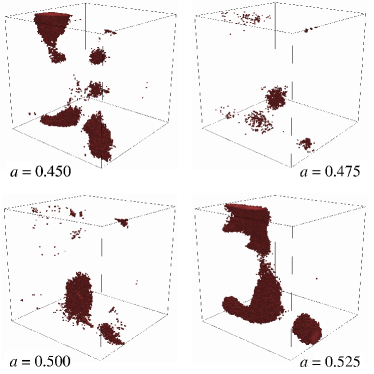
Figure 4: Forming and dissolving mildly nonlinear neutrino overdensities. Simulation cells with a neutrino number density contrast $n_{\nu}/{\bar{n}}_{\nu}\geq 5$ are marked red.

Large-scale neutrino lumps have formed at $a=0.45$. At the intermediate scale factor $a=0.475$, however, the neutrino distribution again is almost homogeneous. Shortly afterwards, the overdensities appear again. Even in their centers, neutrino lumps hardly reach density contrasts above order $10$. The number of structures within the whole $600h^{-1}$Mpc simulation box is very small. The overdensities thus form on a scale of roughly $\lambda\sim 100h^{-1}$Mpc. This is similar to the constant coupling model in which, however, the lumps subsequently shrink to the size of several Megaparsecs and subhalos form Ayaita et al. (2012). In order to guarantee that the simulation box is a representative cosmological volume and to generally avoid box size effects, a larger simulation box would be desirable. Due to the corresponding loss of resolution or, if more cells are used, the increased numerical effort, this analysis is postponed to future work. Our preliminary tests indicate that our findings are robust with respect to box size.

A period of overdensity formation is initiated by a low neutrino equation of state $w_{\nu}\approx 0$. As discussed in the context of the neutrino equation of motion, Eq. (7), the bending of neutrino trajectories and therefore the formation of neutrino overdensities is most effective in this case. The effect is strengthened when the cosmon $\bar{\varphi}$ has come close to the critical value $\varphi_{\text{crit}}$ implying large neutrino masses by Eq. (2). Thereafter, the cosmon “bounces” against the barrier, and $\dot{\bar{\varphi}}$ switches sign becoming negative. The cosmon acceleration $\propto\beta\dot{\varphi}-2H$ in Eq. (8) becomes then positive. Rather than as a damping, it acts as an accelerant and leads to relativistic neutrino velocities high enough such that the neutrinos fly out of the lumps. Consequently, a period of lump formation is followed by a period of lump dissolution. Subsequently, $\dot{\bar{\varphi}}$ turns again positive due to the gradient of the cosmon potential and a new period of lump formation begins.

These cycles of slow-down and speed-up are visualized in Fig. 5.

\psfrag{xlabel}[B][c][.9][0]{scale factor $a$}\psfrag{ylabel}[B][c][.9][0]{average neutrino equation of state $w_{\nu}$}\includegraphics[width=195.12767pt]{wnu.eps}

Figure 5: Evolution of the average equation of state $w_{\nu}$ of neutrinos in the simulation (red solid line) as compared to a purely homogeneous computation (black dashed line).

None of these oscillatory features are visible in a purely homogeneous calculation, which would predict a neutrino equation of state very close to zero. It is the proper treatment of nonlinear perturbations that uncovers why the instability of neutrino perturbations is not “catastrophic” Afshordi et al. (2005). The instability, only present for nonrelativistic neutrinos and leading to the formation of neutrino lumps, is counteracted by the neutrinos turning relativistic again. This constitutes a nonlinear stabilization mechanism.

IV.2 Dark Energy

The periods of nonrelativistic neutrino velocities, $w_{\nu}\approx 0$, are essential for stopping the evolution of the cosmon and ensuring a phase of accelerated expansion (cf. Sec. II.1). The periodically reached relativistic neutrino velocities render the stopping mechanism slightly less effective as they suppress the coupling term $\propto T^{\lambda}_{(\nu)\,\lambda}$ in Eq. (6). This is visible in the evolution of the cosmon equation of state $w_{\varphi}$, cf. Fig. 6.

\psfrag{xlabel}[B][c][.9][0]{scale factor $a$}\psfrag{ylabel}[B][c][.9][0]{cosmon equation of state $w_{\varphi}$}\includegraphics[width=195.12767pt]{wphi.eps}

Figure 6: Evolution of the equation of state $w_{\varphi}$ of Dark Energy in the simulation (red solid line) and in a homogeneous computation (black dashed line). The double peak structure reflects the oscillation of $\varphi$ in an effective potential.

The equation of state $w_{\varphi}$ approaches the cosmological constant value $w_{\Lambda}=-1$ although the full simulation taking the effect of periodically relativistic neutrino velocities into account approaches this value a bit more slowly. Albeit clearly visible, this backreaction effect does not significantly postpone the onset of the accelerated expansion as seen in Fig. 1.

The oscillations in Fig. 6 show a simple pattern. Repeatedly, $w_{\varphi}$ reaches the value $-1$. These are turning points where $\dot{\bar{\varphi}}$ switches sign and thus encounters a zero where $w_{\varphi}=-1$ holds exactly. Narrow and wide minima alternate. The narrow minima occur when $\bar{\varphi}$ bounces against the steep barrier at $\varphi_{\text{crit}}$. The wide minima are related to the other turning point when $\bar{\varphi}$ has climbed the gently inclined scalar self-interaction potential $V(\bar{\varphi})$. The decay of the oscillation amplitude for growing $a$ is a consequence of the damping term $3H\dot{\bar{\varphi}}$ in Eq. (16).

The evolution of the cosmon $\bar{\varphi}$ is reflected in the evolution of the coupling parameter $\beta(\bar{\varphi})$ and the average neutrino mass $m_{\nu}(\bar{\varphi})$, cf. Fig. 7.

\psfrag{xlabel}[B][c][.9][0]{scale factor $a$}\psfrag{ylabel}[B][c][.9][0]{coupling parameter $\beta$}\includegraphics[width=195.12767pt]{beta.eps}

\psfrag{xlabel}[B][c][.9][0]{scale factor $a$}\psfrag{ylabel}[B][c][.9][0]{coupling parameter $\beta$}\psfrag{xlabel}[B][c][.9][0]{scale factor $a$}\psfrag{ylabel}[B][c][.9][0]{average neutrino mass ${\bar{m}}_{\nu}$ [eV]}\includegraphics[width=195.12767pt]{mnu.eps}

Figure 7: Evolution of the coupling parameter $\beta(\varphi)$ and the average neutrino mass $\overline{m_{\nu}(\varphi)}$ in the simulation (red solid line) as compared to a purely homogeneous computation (black dashed line). The nonlinear effects (backreaction) enhance the peaks and lead to a small shift.

They are both proportional to the inverse of $\varphi_{\text{crit}}-\bar{\varphi}$ (which is the distance to the barrier), Eqs. (3) and (2), and reach extrema at the turning points of $\bar{\varphi}$. As the cosmon perturbations $\delta\varphi$ remain small, it is justified to assume $\overline{\beta(\varphi)}\approx\beta(\bar{\varphi})$ and $\overline{m_{\nu}(\varphi)}\approx m_{\nu}(\bar{\varphi})$ for the averages; this is different from the constant coupling case, cf. Sec. II.2. Figure 7 tells us that the backreaction effect is most pronounced at the cusps of the plots. The coupling reaches values $\beta\approx-1.2\times 10^{3}$, and the highest average neutrino mass is $m_{\nu}\approx 0.6$ eV. At the opposite point of the oscillation, the coupling parameter is around $\beta\approx-2\times 10^{2}$, and the mass is at $m_{\nu}\approx 0.15$ eV. As the precise oscillatory pattern will sensitively depend on the chosen model parameters, we conclude that the varying coupling model will not predict a precise value for the present-day neutrino mass but rather a range.

IV.3 Neutrino lump gravitational potential

The only way for cosmological observations to detect the large neutrino overdensities is via the effects of their gravitational potentials. These gravitational potentials have an impact on the evolution of CDM perturbations, in particular on the peculiar velocity field Ayaita et al. (2009). More importantly, they can leave direct observational traces on the cosmic microwave background via the ISW effect. The quantitative results on these gravitational potentials will thus ultimately decide whether the GNQ model will prove viable in the light of various observational constraints. Although answering this question is beyond the scope of this work as it requires an exploration of the model’s parameter space, we show the results obtained for the exemplary set of parameters employed here in Fig. 8.

\psfrag{xlabel}[B][c][.9][0]{scale factor $a$}\psfrag{ylabel}[B][c][.9][0]{relative potential $\Phi_{\nu}(k)/\Phi(k)$}\includegraphics[width=195.12767pt]{potentials.eps}

Figure 8: Comparison between the neutrino-induced gravitational potential $\Phi_{\nu}$ and the total gravitational potential $\Phi$ during the first oscillations at three large comoving scales.

The neutrino-induced gravitational potential $\Phi_{\nu}$ is subdominant, by two orders of magnitude, compared to the CDM potential $\Phi_{m}$. More precisely, the figure shows the dimensionless spectra $\Phi_{\nu}(k)$, $\Phi_{m}(k)$ (cf. also Ref. Ayaita et al. (2012)).

Between the different comoving scales, we observe a phase shift. During the dissolution process, small scales are washed out more rapidly than large scales. Inversely, during the formation process, small-scale perturbations build up faster.

V Physical picture

V.1 Effective cosmon dynamics

Our aim is an analytic understanding of the time evolution of the average cosmon field $\bar{\varphi}$ in the presence of inhomogeneous and possibly rapidly moving neutrinos. For this purpose, we employ an effective potential $V_{\text{eff}}(\bar{\varphi})$ which depends, in addition to $\bar{\varphi}$, also on a characteristic neutrino momentum $p$ and the average neutrino density ${\bar{n}}_{\nu}$. Both, $p$ and ${\bar{n}}_{\nu}$ may depend on the scale factor $a$ or other cosmological quantities, but are assumed to show no explicit dependence on $\bar{\varphi}$. The time evolution of $\bar{\varphi}$ will then be governed by the equation of motion

$$\ddot{\bar{\varphi}}+3H\dot{\bar{\varphi}}+V_{\text{eff}\,,\bar{\varphi}}(\bar{\varphi})=0.$$ (24)

The derivative $V_{\text{eff}\,,\bar{\varphi}}$ is composed of the self-interaction part $V_{,\bar{\varphi}}$ and a contribution from the cosmon-neutrino interaction given by the right-hand side of Eq. (16),

$$V_{\text{eff}\,,\bar{\varphi}}(\bar{\varphi})=V_{,\bar{\varphi}}(\bar{\varphi})+\overline{\beta T_{(\nu)}}.$$ (25)

For an estimate of the coupling term, we assume that it can be written in the form

$$\overline{\beta T_{(\nu)}}=\frac{\partial{\bar{m}}_{\nu}(\bar{\varphi})}{\partial\bar{\varphi}}\,\frac{{\bar{n}}_{\nu}}{\bar{\gamma}},$$ (26)

with ${\bar{m}}_{\nu}(\bar{\varphi})$ the average neutrino mass and ${\bar{n}}_{\nu}(a)\propto a^{-3}$ the (known) average neutrino number density. The exact formula would be a sum over individual particle contributions, where the right-hand side for each particle is just as in Eq. (26) if we replace $\bar{\gamma}$ by the usual Lorentz factor $\gamma$ (cf. Ref. Ayaita et al. (2012)). The effective Lorentz factor $\bar{\gamma}$ is assumed to depend on $\bar{\varphi}$ only through ${\bar{m}}_{\nu}(\bar{\varphi})$. Then, dimensional analysis implies that $\bar{\gamma}$ is a function of the combination $p^{2}/{\bar{m}}_{\nu}^{2}(\bar{\varphi})$, where $\boldsymbol{p}$ is some appropriate characteristic momentum for the neutrinos and $p=\sqrt{\boldsymbol{p}^{2}}$. In principle, the difference between the average of $\partial m_{\nu}/\partial\varphi$ and $\partial{\bar{m}}_{\nu}/\partial\bar{\varphi}$ is included in the factor $\bar{\gamma}$. For the present scenario, our numerical simulations show that these two quantities are approximately equal since the neutrino density perturbation sourcing the cosmon perturbation $\delta\varphi$ never reaches large values during the cosmic evolution.

The effective potential can now be defined as

$$V_{\text{eff}}(\bar{\varphi})=V(\bar{\varphi})+{\bar{n}}_{\nu}\,{\bar{m}}_{\nu}(\bar{\varphi})\,\hat{\gamma},$$ (27)

with $\hat{\gamma}$ related to $\bar{\gamma}$ by

$$\hat{\gamma}+\frac{\partial\hat{\gamma}}{\partial\ln{\bar{m}}_{\nu}}=\frac{1}{\bar{\gamma}}.$$ (28)

Employing that $\hat{\gamma}$ is a dimensionless function of $p^{2}/{\bar{m}}_{\nu}^{2}$, Eq. (28) follows directly from Eq. (24) and the definition of $\bar{\gamma}$ by Eq. (26). For the case of a free particle with

$${\bar{\gamma}}^{2}=1+\frac{p^{2}}{{\bar{m}}_{\nu}^{2}(\bar{\varphi})},$$ (29)

one obtains $\hat{\gamma}=\bar{\gamma}$. For more general momentum distributions of neutrinos, the functions $\bar{\gamma}(p^{2}/{\bar{m}}_{\nu}^{2})$ and $\hat{\gamma}(p^{2}/{\bar{m}}_{\nu}^{2})$ may be somewhat more complicated, but the qualitative relation remains similar.

We next need to understand the time evolution of the characteristic neutrino momentum $p$. We distinguish for each oscillation period two stages. The first stage is characterized by the importance of inhomogeneities in the cosmon field, occurring when $\bar{\varphi}$ is close to the critical value $\varphi_{\text{crit}}$. There, the neutrino mass is close to its maximum, and $p^{2}\ll{\bar{m}}_{\nu}^{2}(\bar{\varphi})$ such that $\bar{\gamma}\approx\hat{\gamma}\approx 1$. The spatial cosmon gradients in the neutrino equation of motion, Eq. (7), lead to the growth of $p^{2}$ and to the formation of neutrino overdensities. We identify a second stage when $\bar{\varphi}$ is no longer close to $\varphi_{\text{crit}}$. Here, inhomogeneities in the cosmon field are no longer decisive, and the overall dynamics is dominated by cosmon acceleration. We will argue that, for this second stage, $p^{2}$ is (almost) conserved. The effective potential $V_{\text{eff}}(\bar{\varphi})$ then only depends on the value of $p^{2}$ that has been reached during the first stage.

For a single particle in a homogeneous background, the combination $\boldsymbol{p}/a$ is conserved due to translation symmetry. In the absence of gravity (for constant $a$), this follows directly from the neutrino equation of motion, Eq. (7), in the case where spatial gradients of $\varphi$ can be neglected,

$$\frac{\mathrm{d}u^{k}}{\mathrm{d}t}=\beta(\bar{\varphi})\,\dot{\bar{\varphi}}\,u^{k}.$$ (30)

This equation of motion conserves the relativistic momentum $\boldsymbol{p}=m_{\nu}(\bar{\varphi})\,\boldsymbol{u}$. Beyond small effects from the expanding scale factor, any additional change of $p$ has to arise from inhomogeneities. These are small during the second stage.

We plot, in Fig. 9, the effective potential given by Eq. (29), taking the parameters from the simulation around the oscillation at $a\approx 0.5$.

\psfrag{xlabel}[B][c][.9][0]{cosmon value $\bar{\varphi}-\varphi_{\text{crit}}$}\psfrag{ylabel}[B][c][.9][0]{effective potential $V_{\text{eff}}(\bar{\varphi})/V(0)$}\includegraphics[width=195.12767pt]{veff.eps}

Figure 9: Effective cosmon potential $V_{\text{eff}}(\bar{\varphi})$ for the nonlinear (red solid) and the homogeneous case (black dashed). For comparison, we also show the self-interaction potential $V(\bar{\varphi})$ (gray dotted) without the effects of the cosmon-neutrino coupling. Units of $V$ are set by the normalization factor $V(0)=1.06\times 10^{-7}\text{Mpc}^{-2}$.

The homogeneous computation that we show as a comparison employs $p=0$. The cosmon $\bar{\varphi}$ oscillates around the minimum of the effective potential according to the effective equation of motion, Eq. (24). The asymmetry of the effective potential explains the double peak structure discussed in Sec. IV.2.

The identification of the characteristic neutrino momentum $p$ as the decisive parameter for the cosmon dynamics opens the door to effective descriptions no longer relying on a full cosmological simulation. For example, the momentum build-up during overdensity formation might be estimated in a suitable spherical collapse approach Wintergerst and Pettorino (2010) or even with an adaption of linear perturbation theory. A detailed investigation of these routes is beyond the scope of this note and left for future work.

V.2 Effective neutrino dynamics

Within the structure formation cycle, we consider first the period of approximate homogeneity for which the cosmon acceleration has violently disrupted the previously formed overdensities. During this period, the effects of the mutual attraction of the neutrinos are suppressed due to their relativistic velocities. The decisive conserved quantity is the relativistic momentum $p$ whose value is determined by the preceding period of overdensity formation. Of course, $p$ shrinks due to the ordinary Hubble damping; but this effect is small because it is linked to a much larger time scale, $1/H$, as compared to the dynamic timescale of the cosmon-neutrino coupling, which is $1/|\beta\dot{\bar{\varphi}}|$. During this approximately homogeneous phase, the neutrinos influence the cosmon evolution via the effective potential $V_{\text{eff}}(\bar{\varphi};p)$ according to Eq. (24). For large enough $\varphi_{\text{crit}}-\bar{\varphi}$, there will be a turnaround with $\bar{\varphi}$ increasing subsequently until a new phase of lump formation sets in.

We next discuss the phase of lump formation. During this phase, the influence of neutrino inhomogeneities on the effective potential $V_{\text{eff}}(\bar{\varphi};p)$ is small, and we may use the homogeneous computation ($p=0$). Indeed, when $\bar{\varphi}$ comes close to $\varphi_{\text{crit}}$ (where overdensities form), the neutrinos become nonrelativistic due to their rapidly growing masses, and the homogeneous computation of $V_{\text{eff}}$ is fairly accurate. In principle, the validity of the homogeneous computation could be spoiled by the type of backreaction effects encountered in the constant coupling model, cf. Sec. II.2, where the local cosmon value effectively freezes and no longer follows the homogeneous component. We do not observe these effects, here, since the neutrino overdensities never become large.

Taking things together, we end with a rather simple qualitative understanding of the role of nonlinearities. The evolution of the cosmon average field $\bar{\varphi}$ is rather independent of the details of the lump formation process. We only need to understand the small increase of the characteristic neutrino momentum $p$ during each phase of lump formation. On the other hand, for the stages of lump formation, the cosmon field dynamics can be approximated by neglecting the backreaction effects (e. g. $p=0$ in $V_{\text{eff}}$).

The details of the stages of lump dissolution are not crucial because the overall picture there is just given by the conservation of the momentum distribution $f(\boldsymbol{p})$. The latter provides an explanation for some of the observations made in Sec. IV.1. Not only did the lumps periodically appear and disappear – they occurred roughly in a similar shape as in the preceding period. Furthermore, the periodic minima in the neutrino equation of state $w_{\nu}$, cf. Fig. 5, reach higher values every time rather than always shrinking to $w_{\nu}=0$. This cannot be explained by the spatial distribution of the neutrino density which is, to a very good approximation, homogeneous after each dissolution phase. It is the conservation of the neutrino momentum distribution $f(\boldsymbol{p})$ during the dissolution process that tells us that the overdensity formation process does not start from a clean state. When the overdensities are just to form again, the neutrino velocities are already pointing to the – previous and next – overdensities’ centers. The momentum build-up during overdensity formation then adds up with the preceding momentum. In each iteration, the momentum thus takes on larger values, and the equation of state after overdensity formation has increased compared to the last iteration.

Rather than describing the process of overdensity formation in an adapted linear perturbation theory or spherical collapse scheme, we content ourselves here with a brief qualitative discussion explaining the main effects. This will make plausible our finding that the neutrino-induced gravitational potentials remain small compared to those of CDM (cf. Fig. 8). A refined analysis will be the subject of future work. The overdensities form when the cosmon comes close to $\varphi_{\text{crit}}$, the barrier in the effective potential $V_{\text{eff}}$. The spatial cosmon gradients become important compared to the time derivative. The coupling parameter $\beta$ reaches order $-10^{3}$, cf. Fig. 7.

Although the resulting forces on the neutrinos are $2\beta^{2}\sim 10^{6}$ times stronger than gravity, several factors hinder the formation of highly concentrated lumps. First, the period of time during which the cosmon is close to $\varphi_{\text{crit}}$ and the neutrinos are nonrelativistic is limited to roughly $\Delta a\sim 10^{-2}$, cf. Figs. 5 and 6. The nonrelativistic neutrinos are not fast enough to form overdensities beyond roughly $\delta_{\nu}\sim 10^{-2}$ as seen in the simulation. After the cosmon has bounced against the barrier and $\dot{\bar{\varphi}}$ is negative, the cosmon acceleration increases all neutrino velocities along their respective directions of motion. At first, the overdensities continue to grow as the neutrino velocities were on average, during the nonrelativistic period, targeting towards the centers of the forming overdensities. This explains why the maxima of the neutrino-induced gravitational potential occur at later times than the bouncing of $\bar{\varphi}$ against the barrier, cf. Fig. 8. However, during the cosmon acceleration, the neutrino masses rapidly decrease. Consequently, although the number overdensities grow, the effect on the gravitational potential is only moderate. At its maxima, the large-scale gravitational potential induced by neutrinos is only at the percent level compared to the CDM potential.

For small scales, the neutrinos form even less overdensities compared to $\delta_{m}$. The relative importance of the neutrino gravitational potential therefore decreases towards smaller length scales.

VI Conclusion

The Growing Neutrino Quintessence model with a field-dependent coupling $\beta(\varphi)$ shows violent nonlinear dynamics of the coupled cosmon-neutrino fluid, and yet an overall phenomenology similar to the standard $\Lambda$CDM picture. The accelerated expansion is almost the same as for $\Lambda$CDM (cf. Fig. 1), while large-scale neutrino overdensities remain small enough so that their induced gravitational potentials are subdominant to those of cold dark matter. At the fundamental level, however, the model is not anywhere near $\Lambda$CDM. Rather than being a parameter, the present Dark Energy density results from the stop of a scaling solution by a cosmological trigger event, namely neutrinos becoming nonrelativistic. In the process, the coupling parameter between the neutrinos and Dark Energy dynamically reaches order $\beta(\varphi)\sim-10^{3}$ (cf. Fig. 7), inducing an attraction between neutrinos $10^{6}$ times stronger than gravity. This may serve as an example that a standard overall phenomenology still leaves room for new physics, without unnaturally small parameters.

The average neutrino mass $m_{\nu}$ is small in the early universe. For most of the cosmological evolution, the Dark Energy scalar field rolls down steadily its potential towards larger values, and the average neutrino mass grows with time. In the recent epoch, however, the cosmon field value oscillates and so do the neutrino masses. For the investigated parameters, $m_{\nu}$ oscillates between about $0.15$ eV and $0.6$ eV (cf. Fig. 7). Nonrelativistic neutrinos experience an attractive force due to the coupling $\beta(\varphi)$ substantially stronger than gravity. Furthermore, Hubble damping is replaced by cosmon acceleration.

The violent nonlinear behavior of neutrino perturbations manifests itself in the repeated rapid formation and dissolution of large-scale overdensities (cf. Fig. 4). Rather than becoming nonrelativistic once and for all, the neutrinos are accelerated to relativistic velocities periodically (cf. Fig. 5). This effectively stabilizes the evolution of perturbations, and the “catastrophic” instability first discussed in the context of MaVaNs is avoided Afshordi et al. (2005). The (short-lived) overdensities induce oscillating gravitational potentials, whose relative strength compared to those of cold dark matter remains at the percent level (cf. Fig. 8).

By virtue of the coupling between Dark Energy and the neutrinos, the nonlinear dynamics of neutrino perturbations exert a backreaction effect on the evolution of Dark Energy at the background level. Relativistic neutrino velocities reduce the strength of the effect of the coupling and thereby weaken the Dark Energy stopping mechanism. Although the backreaction is clearly visible quantitatively for the equations of state of individual components, it does not alter the qualitative picture with a usual crossover to the accelerated expansion epoch (cf. Fig. 6). For our parameter set, the backreaction effect becomes negligible for the evolution of the overall energy fraction for the coupled cosmon-neutrino fluid which constitutes Dark Energy, see Fig. 1. This finding is in contrast to the constant coupling model in which stable neutrino lumps form and effectively decouple from the homogeneous component. There, a much stronger backreaction effect substantially postpones the onset of the accelerated expansion Ayaita et al. (2012).

We have obtained our numerical results from an $N$-body based simulation technique Ayaita et al. (2012), specifically developed for the Growing Neutrino Quintessence model, together with a Newton-Gauß-Seidel solver for the local Dark Energy perturbations Puchwein et al. (2013). Our method (described in Sec. III) has allowed to show, for the first time, the nonlinear evolution of the model until redshift zero. Earlier attempts had to stop at $z\approx 1$ and were restricted to the technically simpler constant coupling model Baldi et al. (2011); Ayaita et al. (2012). Still, the very strong coupling parameters and the violent perturbation evolution have so far prevented a scan of the model’s parameter space for the field-dependent coupling model. This, however, would be a decisive step towards a confrontation of the model with observational constraints. Further efforts are required to render the numerical method faster and more robust.

A complementary road consists in a semi-analytical approach allowing for a simplified yet reliable description of the cosmological dynamics. In the constant coupling model, this had inspired the physical picture of a cosmon-neutrino lump fluid Ayaita et al. (2013). We have laid the ground here for such an effective description of the field-dependent coupling model, whose cornerstones we have explained in Sec. V. In periods during which the cosmon evolves rapidly, the neutrino momenta are approximately conserved. This conservation has enabled us to define an effective self-interaction potential for the scalar field $V_{\text{eff}}(\varphi)$ (cf. Fig. 9) that fully describes the evolution of the homogeneous Dark Energy. For the neutrino component, our findings motivate an adapted spherical collapse approach that would allow to estimate the momentum build-up during the overdensity formation process. Such a semi-analytical approach will be shaped along with the continuing work on the numerical simulation method.

Despite the important steps still to be done, the overall picture for the confrontation of Growing Neutrino Quintessence with observations already takes a clear shape. For the varying coupling $\beta(\varphi)$ and the parameter set chosen for the present paper, the background evolution is essentially indistinguishable from the $\Lambda$CDM model. (The small fraction of Early Dark Energy can be further reduced by a larger value of the parameter $\alpha$.) Also the gravitational potential induced by the neutrino lumps seems too small for an easy observational detection. Such models appear to be compatible with present observations to the same degree as $\Lambda$CDM. On the other side, the models with constant coupling $\beta$ may allow for parameters such that the present Dark Energy can be adjusted to the observed value. In this case, we expect much stronger neutrino-induced gravitational potentials, observable by the ISW effect or other tests. It is obvious that, for part of the parameter space, Growing Neutrino Quintessence deviates substantially from observation and the $\Lambda$CDM model. Large parameter regions lie between the two extremes. They will allow for clear signals for future observations without being inconsistent with present observations. The cosmic neutrino background may finally become observable.