Combining isotonic regression and EM algorithm to predict genetic risk under monotonicity constraint

Abstract

In certain genetic studies, clinicians and genetic counselors are interested in estimating the cumulative risk of a disease for individuals with and without a rare deleterious mutation. Estimating the cumulative risk is difficult, however, when the estimates are based on family history data. Often, the genetic mutation status in many family members is unknown; instead, only estimated probabilities of a patient having a certain mutation status are available. Also, ages of disease-onset are subject to right censoring. Existing methods to estimate the cumulative risk using such family-based data only provide estimation at individual time points, and are not guaranteed to be monotonic or nonnegative. In this paper, we develop a novel method that combines Expectation–Maximization and isotonic regression to estimate the cumulative risk across the entire support. Our estimator is monotonic, satisfies self-consistent estimating equations and has high power in detecting differences between the cumulative risks of different populations. Application of our estimator to a Parkinson’s disease (PD) study provides the age-at-onset distribution of PD in PARK2 mutation carriers and noncarriers, and reveals a significant difference between the distribution in compound heterozygous carriers compared to noncarriers, but not between heterozygous carriers and noncarriers.

copyrightownerIn the Public Domain

, , , , and

t2Supported by the Huntington’s Disease Society of America, Human Biology Project Fellowship. t5Supported by NS036630 Parkinson disease Foundation, UL1 RR024156. t6Supported by NIH Grant NS073671.

1 Introduction

In genetic epidemiology studies [Struewing et al. (1997), Marder et al. (2003), Goldwurm et al. (2011)], family history data is collected to estimate the cumulative distribution function of disease onset in populations with different risk factors (e.g., genetic mutation carriers and noncarriers). Such estimates provide crucial information to assist clinicians, genetic counselors and patients to make important decisions such as mastectomy [Grady, Parker-Pope and Belluck (2013)]. The family history data, however, raises serious challenges when estimating the cumulative risk. First, a family member’s exact risk factor is unknown; the only available information is the estimated probabilities that a family member has each risk factor. Second, ages of disease onset are subject to censoring due to patient drop-out or loss to follow-up. For such family history data, the cumulative risk of disease is thus a mixture of cumulative distributions for the risk factors with known mixture probabilities. While different parametric and nonparametric estimators have been proposed for estimating these mixture data distribution functions, they are not guaranteed to be monotonic or nonnegative, two principle features of distribution functions. Most of these estimators also examine the mixture distributions only at individual time points, rather than at a range of time points. To overcome these challenges, we develop a novel, simultaneous estimation method which combines isotone regression [Barlow et al. (1972)] with an Expectation–Maximization (EM) algorithm. Our algorithm is based on the binomial likelihood at all observations [Huang, Qin and Zou (2007), Ma and Wang (2014)], and yields estimated distribution functions that are nonnegative, monotone, consistent, efficient and that provide estimates of the cumulative risk over a range of time points.

Family history data is often collected when studying the risk of disease associated with rare mutations [Struewing et al. (1997), Marder et al. (2003), Wang et al. (2008), Goldwurm et al. (2011)]. For example, estimating the probability that Ashkenazi Jewish women with specific mutations of BRCA1 or BRCA2 will develop breast cancer [Struewing et al. (1997)], estimating the survival function from relatives of Huntington’s Disease probands with expanded C-A-G repeats in the huntingtin gene [Wang, Garcia and Ma (2012)] and, in this paper, estimating age at onset of Parkinson’s disease in carriers of PARK2 mutations (Section 1.1).

In all these cases, a sample of (usually diseased) subjects referred to as probands are genotyped. Disease history in the probands’ first-degree relatives, including age at onset of the disease, is obtained through validated interviews [Marder et al. (2003)]. Because of practical considerations, including high costs or unwillingness to undergo genetic testing, the relatives’ genotype information is not collected. Instead, the probability that the relative has the mutation or not is computed based on the relative’s relationship to the proband and the proband’s mutation status [Khoury, Beaty and Cohen (1993), Section 8.4]. Thus, the distribution of the relative’s age at onset of a disease is a mixture of genotype-specific distributions with known, subject-specific mixing proportions.

A first attempt at estimating the mixture distribution functions was based on assuming parametric or semiparametric forms [Wu, Ma and Casella (2007)] for the underlying mixture densities. To avoid model misspecification, however, nonparametric estimators such as the nonparametric maximum likelihood estimator (NPMLE) were also proposed. While in many situations the NPMLEs are consistent and efficient, they are neither for the mixture model [Wang, Garcia and Ma (2012), Ma and Wang (2014)]. As improvements over the NPMLEs, Wang, Garcia and Ma (2012) and Ma and Wang (2014) proposed consistent and efficient nonparametric estimators based on estimating equations. The estimators stem from casting the problem into a semiparametric theory framework and identifying the efficient estimator. The resulting estimator, however, can have computational difficulties when the data is censored, as it uses inverse probability weighting (IPW) and augmented IPW to estimate the mixture distribution functions [Wang, Garcia and Ma (2012)]. The weighting function involves a Kaplan–Meier estimator which can result in unstable estimation because the weighting function can be close to zero in the right tail. There is also no guarantee that the resulting estimator is monotonic or nonnegative, thus, a post-estimate adjustment was implemented to ensure monotonicity.

In this paper, we propose a novel nonparametric estimator that is neither complex nor computationally intensive, and yields a genuine distribution for the mixture data problem under the monotonicity constraint of a distribution function. Providing nonparametric estimators for survival functions under ordered constraints has received considerable attention recently [Park, Taylor and Kalbfleisch (2012), El Barmi and McKeague (2013)], but the emphasis has been on nonmixture data. The method we propose is applicable to mixture data. Our method is motivated from a real-world study on genetic epidemiology of Parkinson’s disease (see Section 1.1) and is based on maximizing a binomial likelihood simultaneously at all observations [Huang, Qin and Zou (2007)]. Our method involves combining an EM algorithm and isotone regression [Ayer et al. (1955)] so that monotonicity is ensured. We demonstrate that our estimator is consistent, satisfies self-consistent estimating equations and yields large power in detecting differences between the distribution functions in the mixture populations. Our estimator is easy to implement and, for nonmixture data, we show that our method coincides with the NPMLE.

1.1 CORE-PD study to estimate the risk of PARK2 mutations

Parkinson’s disease (PD) is a neurodegenerative disorder of the central nervous system that results in bradykinesia, tremors and problems with gait. PD mostly affects the elderly 50 and older, but early onset cases do occur and are hypothesized to be a result of genetic risk factors. Mutations in the PARK2 gene [Kitada et al. (1998), Hedrich et al. (2004)] are the most common genetic risk factor for early-onset PD [Lücking et al. (2000)] and may be a risk factor for late onset [Oliveira et al. (2003)]. While mutations in the PARK2 gene are rare, genetic or acquired defects in Parkin function may have far-reaching implications for the understanding and treatment of both familial and sporadic PD.

To understand the effects of mutations in the PARK2 gene, the Consortium on Risk for Early Onset PD (CORE-PD) study was begun in 2004 [Marder et al. (2010)]. Experienced neurologists performed in-depth examinations (i.e., neurological, cognitive, psychiatric assessments) of proband participants, a subset of noncarriers, and some of the first-degree relatives of probands and noncarriers. For relatives who were not examined in person, their PARK2 genotypes were not available, but their age at onset of PD was obtained through systematic family history interviews [Marder et al. (2003)]. Based on this family history data, the objective then is to determine the age-specific cumulative risk of PD in PARK2 mutation carriers and noncarriers. The results will help patients interpret a positive test result both in deciding treatment options and making important life decisions such as family planning.

The remaining sections of this paper are as follows. Section 2 describes our proposed estimator which involves maximizing a binomial log-likelihood with an EM algorithm. We demonstrate that the ensuing estimator solves a self-consistent estimating equation and is consistent for complete and right censored data. We demonstrate in Section 3 that we can reformulate the estimator using a different EM algorithm, for which we can apply the pool adjacent violators algorithm (PAVA) from isotone regression to yield a nonnegative and monotonic estimator. We demonstrate the advantages of our new estimator over current ones through extensive simulation studies in Section 4. We apply our estimator to the CORE-PD study in Section 5 and conclude the paper in Section 6. Technical details are in the Appendix, and additional numerical results are available in the supplementary material [Qin et al. (2014)].

2 Binomial likelihood estimation

To simplify the presentation, we focus on a mixture distribution with two components; the techniques presented can be easily extended to more than two components.

For $i=1,\ldots,n$, we observe a quantitative measure $S_{i}$ known to come from one of $p=2$ populations with corresponding distributions $F_{1},F_{2}$ and densities $dF_{1},dF_{2}$. For example, in the Parkinson’s disease study, $S_{i}$ is the age of disease onset, $F_{1}$ is the distribution for the PARK2 mutation carrier group, and $F_{2}$ is for the noncarrier group. The exact population to which $S_{i}$ belongs is unknown (i.e., we do not know whether a family member is a mutation carrier or noncarrier), but one can estimate the probability $q_{ki}$ that $S_{i}$ was generated from the $k$th population, $k=1,2$. We suppose the mixture probability ${\mathbf{Q}}_{i}$ has a discrete distribution, denoted as $p_{{\mathbf{Q}}}({\mathbf{q}}_{i})$, with finite support ${\mathbf{u}}_{1},\ldots,{\mathbf{u}}_{m}$. We also suppose that $q_{1i}+q_{2i}=1$ and, hence, sometimes write $q_{1i}\equiv\lambda_{i}$ and $q_{2i}\equiv 1-\lambda_{i}$. In this case, instead of referring to the discrete distribution $p_{{\mathbf{Q}}}({\mathbf{q}}_{i})$, we simply refer to the distribution of $\lambda_{i}$, denoted as $\eta(\lambda_{i})$. Furthermore, $S_{i}$ is subject to right-censoring, so we observe $X_{i}=\min(S_{i},C_{i})$, where $C_{i}$ is a random censoring time independent of $S_{i}$. We let $G(\cdot)$ denote the survival function of $C_{i}$ and $dG(\cdot)$ its corresponding density. Last, we let $\Delta_{i}=I(S_{i}\leq C_{i})$ denote the censoring indicator.

Our objective is to use the independent, identically distributed (i.i.d.) data $({\mathbf{Q}}_{i}={\mathbf{q}}_{i},X_{i}=x_{i},\Delta_{i}=\delta_{i})$ to form a nonparametric estimator of ${\mathbf{F}}(t)=\{F_{1}(t),F_{2}(t)\}^{T}$ that is consistent, monotone on the support of $S_{i}$ and efficient. Identifiability of ${\mathbf{F}}(t)$ is ensured since the mixture probabilities are assumed known and ${\mathbf{Q}}_{i}$ are not all the same [Wang et al. (2007)]. In fact, if $Q_{i}$ has at least $k$ distinguished the support points, then the model is identifiable. To estimate ${\mathbf{F}}(t)$, we first consider the nonparametric log-likelihood

$$\sum_{i=1}^{n}\log\bigl{(}p_{{\mathbf{Q}}}({\mathbf{q}}_{i})\bigl{\{}{\mathbf{q}}_{i}^{T}{\mathbf{d}}{\mathbf{F}}(x_{i})G(x_{i})\bigr{\}}^{\delta_{i}}\bigl{[}\bigl{\{}1-{\mathbf{q}}_{i}^{T}{\mathbf{F}}(x_{i})\bigr{\}}\,dG(x_{i})\bigr{]}^{1-\delta_{i}}\bigr{)}.$$

Because $p_{{\mathbf{Q}}}(q_{i})$ is independent of the estimation of ${\mathbf{F}}(t)$, and the censoring times are random, the log-likelihood above simplifies to

$$\sum_{i=1}^{n}\log\bigl{[}\bigl{\{}{\mathbf{q}}_{i}^{T}{\mathbf{d}}{\mathbf{F}}(x_{i})\bigr{\}}^{\delta_{i}}\bigl{\{}1-{\mathbf{q}}_{i}^{T}{\mathbf{F}}(x_{i})\bigr{\}}^{1-\delta_{i}}\bigr{]}.$$ (1)

Different maximizations of (1) result in the commonly used NPMLEs (see Appendix .1). Unfortunately, for the mixture data problem, they turn out to be inconsistent or inefficient [Ma and Wang (2012)].

2.1 Motivation for binomial likelihood formulation

As an improvement over the NPMLEs, we consider a binomial likelihood estimator. To motivate this estimator, we first consider a nonmixture model without censoring. That is, we observe independent observations $S_{1},\ldots,S_{n}$ generated from a common distribution $F$. Without loss of generality, we suppose $S_{1}\leq S_{2}\leq\cdots\leq S_{n}$ (i.e., ties may occur). We demonstrate that, in this setting, the NPMLE and the binomial likelihood estimator of $F$ are the same. Thus, because the NPMLE is most efficient in this setting, the binomial likelihood estimator is as well.

For nonmixture data without censoring, the nonparametric estimator of $F$ maximizes

$$\sum_{i=1}^{n}\log\,dF(s_{i})$$

with respect to $dF(s_{i})$ subject to $\sum_{i=1}^{n}\,dF(s_{i})=1$ and $dF(s_{i})\geq 0$. From first principles, the maximizer is the well-known empirical distribution function, $\widehat{F}_{n}(t)=n^{-1}\sum_{i=1}^{n}I(s_{i}\leq t)$.

On the other hand, the empirical distribution function is also the maximizer of the following binomial log-likelihood. For distinctive time points $t_{1}<t_{2}<\cdots<t_{h}$ and each $S_{i}$, denote a success if $S_{i}>t_{j}$ and a failure if $S_{i}\leq t_{j}$ $i=1,\ldots,n$, $j=1,\ldots,h$. The probability of a success is $\bar{F}(t_{j}):=1-F(t_{j})$, and the probability of a failure is $F(t_{j})$. The times $t_{1},\ldots,t_{h}$ can be arbitrary, but are typically chosen to span the support of the events $S_{i}$ so as to estimate the cumulative distribution function over the full support.

Accounting for all possible successes and failures, the binomial log-likelihood is

$$\sum_{j=1}^{h}\sum_{i=1}^{n}\bigl{\{}I(s_{i}\leq t_{j})\log F(t_{j})+I(s_{i}>t_{j})\log\bar{F}(t_{j})\bigr{\}}.$$

Maximizing the above with respect to each $F(t_{j})$ and subject to the monotonic constraint $F(t_{1})\leq F(t_{2})\leq\cdots\leq F(t_{h})$ gives

$$\widehat{F}_{n}(t_{j})=n^{-1}\sum_{i=1}^{n}I(s_{i}\leq t_{j}),\qquad j=1,\ldots,h.$$

However, this is exactly the empirical distribution function which, by definition, satisfies the monotonic constraint.

Therefore, in the nonmixture case, maximizing the nonparametric log-likelihood with respect to $dF$ is equivalent to maximizing the binomial log-likelihood with respect to $F$ subject to the monotonic constraint $F(t_{1})\leq F(t_{2})\leq\cdots\leq F(t_{h})$. Because the two estimators are equivalent and the NPMLE is known to be most efficient, the resulting binomial likelihood estimator is fully efficient. Motivated by this result, we anticipate that maximizing the binomial log-likelihood may yield highly efficient estimators in more general mixture models.

2.2 Binomial likelihood estimator for censored mixture data

We now construct a binomial likelihood estimator for mixture data with censoring. Again, consider arbitrary time points $t_{1}<\cdots<t_{h}$, such that for each event time $S_{i}$, a success occurs if $S_{i}>t_{j}$ and a failure if $S_{i}\leq t_{j}$, $i=1,\ldots,n$, $j=1,\ldots,h$. As in Section 2.1, we allow for ties in the event times $S_{i}$, and choose times $t_{1},\ldots,t_{h}$ to span the support of the event times.

Under censoring, we observe $X_{i}=\min(S_{i},C_{i})$, which means a success, $I(S_{i}>t_{j})$, is unobservable for those subjects who are lost to follow-up before $t_{j}$. A natural approach then is to view the unobserved successes as missing data and to use an EM algorithm to maximize the constructed binomial log-likelihood.

Let $V_{ij}=I(S_{i}>t_{j})$, the unobserved success. For mixture data, when $V_{ij}$ is observable (i.e., noncensored data), we have that $P(V_{ij}=1)=\lambda_{i}\bar{F}_{1}(t_{j})+(1-\lambda_{i})\bar{F}_{2}(t_{j})$ and $P(V_{ij}=0)=\lambda_{i}F_{1}(t_{j})+(1-\lambda_{i})F_{2}(t_{j})$, where $\bar{F}_{k}(t_{j})=1-F_{k}(t_{j})$, $k=1,2$. Considering all time points $t_{1},\ldots,t_{h}$, and all possible successes and failures, the complete data binomial log-likelihood of $\{I(S_{i}>t_{j})\}$, $i=1,\ldots,n$, $j=1,\ldots,h$, is

$$\sum_{j=1}^{h}\sum_{i=1}^{n}\bigl{[}I(s_{i}\leq t_{j})\log\bigl{\{}\lambda_{i}F_{1}(t_{j})+(1-\lambda_{i})F_{2}(t_{j})\bigr{\}}$$

$$\quad\qquad{}+I(s_{i}>t_{j})\log\bigl{\{}\lambda_{i}\bar{F}_{1}(t_{j})+(1-\lambda_{i})\bar{F}_{2}(t_{j})\bigr{\}}\bigr{]}.$$

If $V_{ij}=I(S_{i}>t_{j})$ were observable, we could estimate ${\mathbf{F}}(t_{j})$, $j=1,\ldots,h$, by maximizing the binomial log-likelihood with respect to $F_{1}(t_{j})$ and $F_{2}(t_{j})$. However, because $V_{ij}$ is unobservable, we instead use an EM algorithm for maximization. An EM algorithm at a single $t_{j}$ was given in Ma and Wang (2014), but they did not further pursue it. In fact, Efron (1967) did impute this.

The EM algorithm we propose is an iterative procedure where at the $b$th step the imputed $V_{ij}$ is

$$w_{ij}^{(b)} = E\bigl{\{}I(S_{i}>t_{j})|x_{i}\bigr{\}}$$

$$= I(x_{i}>t_{j})+(1-\delta_{i})I(x_{i}\leq t_{j})\frac{\lambda_{i}\bar{F}_{1}^{(b)}(t_{j})+(1-\lambda_{i})\bar{F}_{2}^{(b)}(t_{j})}{\lambda_{i}\bar{F}_{1}^{(b)}(x_{i})+(1-\lambda_{i})\bar{F}_{2}^{(b)}(x_{i})},$$

based on the observed data $X_{i}=x_{i}$. The E-step is then the imputed binomial log-likelihood

$$\sum_{j=1}^{h}\sum_{i=1}^{n}\bigl{[}\bigl{(}1-w_{ij}^{(b)}\bigr{)}\log\bigl{\{}\lambda_{i}F_{1}(t_{j})+(1-\lambda_{i})F_{2}(t_{j})\bigr{\}}$$

(3)

$$\quad\qquad{}+w_{ij}^{(b)}\log\bigl{\{}\lambda_{i}\bar{F}_{1}(t_{j})+(1-\lambda_{i})\bar{F}_{2}(t_{j})\bigr{\}}\bigr{]}.$$

The M-step then maximizes the above with respect to $F_{1}(t_{j})$ and $F_{2}(t_{j})$; specifically, the M-step involves solving

$$-\sum_{i=1}^{n}\lambda_{i}\frac{w_{ij}^{(b)}-\lambda_{i}\bar{F}_{1}(t_{j})-(1-\lambda_{i})\bar{F}_{2}(t_{j})}{\{\lambda_{i}F_{1}(t_{j})+(1-\lambda_{i})F_{2}(t_{j})\}\{\lambda_{i}\bar{F}_{1}(t)+(1-\lambda_{i})\bar{F}_{2}(t)\}} = 0,$$

$$-\sum_{i=1}^{n}(1-\lambda_{i})\frac{w_{ij}^{(b)}-\lambda_{i}\bar{F}_{1}(t_{j})-(1-\lambda_{i})\bar{F}_{2}(t_{j})}{\{\lambda_{i}F_{1}(t_{j})+(1-\lambda_{i})F_{2}(t_{j})\}\{\lambda_{i}\bar{F}_{1}(t)+(1-\lambda_{i})\bar{F}_{2}(t)\}} = 0,$$

for $j=1,\ldots,h$. The solution to (2.2) leads to the new estimate $F_{1}^{(b+1)}(t_{j})$ and $F_{2}^{(b+1)}(t_{j})$. Iterating the E- and M-steps until convergence leads to the binomial likelihood estimator $\widehat{\mathbf{F}}(t_{j})$, $j=1,\ldots,h$, for censored mixture data. We now make several observations about this proposed estimator.

The estimating equations in (2.2) are optimally weighted [Godambe (1960)] and are, in fact, self-consistent estimating equations [Efron (1967)]. The self-consistency stems from the imputation procedure of the EM algorithm, analogously to the work of Efron (1967). In the special case of right censoring but no mixture, the above approach has a closed-form solution, which is the celebrated Kaplan–Meier estimator [Efron (1967)]. In the general case, it can be shown that the proposed estimator $\widehat{\mathbf{F}}$ is consistent. The proof is trivial if ${\mathbf{F}}$ takes discrete finite many values. On the other hand, if ${\mathbf{F}}$ is a continuous distribution, one may use the law of large sample and Kullback–Leibler information inequality to prove it. Details are given in the Appendix .2. Asymptotics of $\widehat{\mathbf{F}}(t_{j})$ are much more involved, however, and require solving a complex integral equation which is impractical. Hence, inference is usually performed using a Bootstrap approach.

Solving for $\widehat{\mathbf{F}}(t)$ in practice is also a computationally intensive task. No closed-form solution to (2.2) exists, and ensuring monotonicity and nonnegativity of $\widehat{\mathbf{F}}(t)$ would actually require solving (2.2) subject to the constraints $F_{k}(t_{1})\leq F_{k}(t_{2})\leq\cdots\leq F_{k}(t_{h})$, $k=1,2$, for $t_{1}\leq\cdots\leq t_{h}$. Such a constraint only further complicates the already demanding estimation procedure. Still, requiring monotonicity is essential when the data is censored. Without monotonicity, the imputed weights $w_{ij}^{(b)}$ may not be in the range $(0,1)$, which could lead to nonconvergence when solving (2.2). Thus, to ensure monotonicity and avoid the complexities of directly solving (2.2), we now describe another approach for obtaining the binomial likelihood estimator.

3 Genuine nonparametric distribution estimators

To construct a monotone and nonnegative estimator $\widehat{\mathbf{F}}(t)$ at times $t_{1}<\cdots<t_{h}$, we maximize a binomial log-likelihood using a combined EM algorithm and pool adjacent violators algorithm (PAVA). Before describing the new method, we first provide a brief overview of PAVA.

3.1 Pool adjacent violator algorithm

Isotone regression [Barlow et al. (1972)] is the notion of fitting a monotone function to a set of observed points $y_{1},\ldots,y_{n}$ in a plane. Formally, the problem involves finding a vector ${\mathbf{a}}=(a_{1},\ldots,a_{n})^{T}$ that minimizes the weighted least squares

$$\sum_{i=1}^{n}r_{i}(y_{i}-a_{i})^{2}$$

subject to $a_{1}\leq\cdots\leq a_{n}$ for weights $r_{i}>0$, $i=1,\ldots,n$. The solution to this optimization problem is the so-called max-min formula [Barlow et al. (1972)]:

$$\widehat{a}_{j}=\max_{s\leq j}\min_{t\geq j}\frac{\sum_{h=s}^{t}y_{h}r_{h}}{\sum_{h=s}^{t}r_{h}},\qquad j=1,\ldots,n.$$

Rather than solving this max-min formula, the weighted least squares problem is instead solved using PAVA [Ayer et al. (1955), Barlow et al. (1972)], a simple procedure that yields the solution in $O(n)$ time [Grotzinger and Witzgall (1984)]. The history of PAVA, its computational aspects and a fast implementation in R are discussed in de Leeuw, Hornik and Mair (2009). Variations of PAVA implementation include using up-and-down blocks [Kruskal (1964)] and recursive partitioning [Luss, Rosset and Shahar (2010)].

Our idea is to apply PAVA to a variant of our binomial loglikehood and yield a monotone estimator $\widehat{\mathbf{F}}(t)$. It is important to note that we cannot simply apply PAVA to the estimator solving (2.2). The E-step in (2.2) is not in the exponential family, which is a requirement of PAVA [Robertson, Wright and Dykstra (1988)]. Furthermore, applying PAVA to maximize a binomial log-likelihood has been used in current status data [Jewell and Kalbfleisch (2004)], but not in the context of mixture data as we do.

3.2 PAVA-based binomial likelihood estimator for censored mixture data

We now modify the construction of the binomial likelihood estimator for censored mixture data (Section 2.2) so that PAVA may be applied. In our earlier construction (Section 2.2), we viewed the event $I(S_{i}>t_{j})$ as the only missing data, $i=1,\ldots,n$, $j=1,\ldots,h$. Now, we also consider the unobserved population membership as missing. Let $L_{i}$ denote the unobserved population membership for observation $i$.

Analogous to the argument in Section 2.2, we first consider the ideal situation when $L_{i}$ and $I(S_{i}>t_{j})$ are observable. We suppose $L_{i}=1$ when $S_{i}$ is generated from $F_{1}$, and $L_{i}=0$ when $S_{i}$ is generated from $F_{2}$. In this case, $P(L_{i}=1)=\lambda_{i}$ and $P(L_{i}=0)=1-\lambda_{i}$. For mixture data, the probability $S_{i}>t_{j}$ is $\lambda_{i}\bar{F}_{1}(t_{j})$ when $L_{i}=1$ and is $(1-\lambda_{i})\bar{F}_{2}(t_{j})$ when $L_{i}=0$. Likewise, the probability $S_{i}\leq t_{j}$ is $\lambda_{i}F_{1}(t_{j})$ when $L_{i}=1$ and is $(1-\lambda_{i})F_{2}(t_{j})$ when $L_{i}=0$. Therefore, the complete data log-likelihood of $\{L_{i},I(S_{i}\leq t_{j})\},i=1,2\ldots,n,j=1,2,\ldots,h$, is the binomial log-likelihood

$$\ell_{c} = \sum_{j=1}^{h}\sum_{i=1}^{n}\bigl{[}L_{i}I(S_{i}\leq t_{j})\log\bigl{\{}\lambda_{i}F_{1}(t_{j})\bigr{\}}+L_{i}I(S_{i}>t_{j})\log\bigl{\{}\lambda_{i}\bar{F}_{1}(t_{j})\bigr{\}}$$

$$\quad\qquad{}+(1-L_{i})I(S_{i}\leq t_{j})\log\bigl{\{}(1-\lambda_{i})F_{2}(t_{j})\bigr{\}}$$

$$\hskip 78.0pt\qquad{}+(1-L_{i})I(S_{i}>t_{j})\log\bigl{\{}(1-\lambda_{i})\bar{F}_{2}(t_{j})\bigr{\}}\bigr{]}.$$

However, neither the population membership $L_{i}$ nor the event $I(S_{i}>t_{j})$ are available. Hence, these values must be imputed, and an EM algorithm will be used for maximization.

At the $b$th step of the EM algorithm, we compute $E\{L_{i}I(S_{i}\leq t_{j})|x_{i}\}=E\{L_{i}|S_{i}\leq t_{j}\}E\{I(S_{i}\leq t_{j})|x_{i}\}$ and $E\{L_{i}I(S_{i}>t_{j})|x_{i}\}=E\{L_{i}|\break S_{i}>t_{j}\}E\{I(S_{i}>t_{j})|x_{i}\}$ based on observed data $X_{i}=\min(S_{i},C_{i})$ with $X_{i}=x_{i}$. We found earlier that $E\{I(S_{i}>t_{j})|x_{i}\}=w_{ij}^{(b)}$ as defined in (2.2). Using a similar calculation, we obtain

$$u_{ij}^{(b)} \equiv E(L_{i}|S_{i}\leq t_{j})=\frac{\lambda_{i}F_{1}^{(b)}(t_{j})}{\lambda_{i}F_{1}^{(b)}(t_{j})+(1-\lambda_{i})F_{2}^{(b)}(t_{j})},$$

$$v_{ij}^{(b)} \equiv E(L_{i}|S_{i}>t_{j})=\frac{\lambda_{i}\bar{F}_{1}^{(b)}(t_{j})}{\lambda_{i}\bar{F}_{1}^{(b)}(t_{j})+(1-\lambda_{i})\bar{F}_{2}^{(b)}(t_{j})}.$$

Therefore, at the $b$th step, with observed data ${\mathbf{O}}^{(b)}=\{X_{i}\},i=1,\ldots,n$, the E-step is

$$E\bigl{(}\ell_{c}|{\mathbf{O}}^{(b)}\bigr{)} = \sum_{j=1}^{h}\sum_{i=1}^{n}\bigl{[}u_{ij}^{(b)}\bigl{(}1-w_{ij}^{(b)}\bigr{)}\log\bigl{\{}\lambda_{i}F_{1}(t_{j})\bigr{\}}+v_{ij}^{(b)}w_{ij}^{(b)}\log\bigl{\{}\lambda_{i}\bar{F}_{1}(t_{j})\bigr{\}}$$

$$\quad\qquad{}+\bigl{(}1-u_{ij}^{(b)}\bigr{)}\bigl{(}1-w_{ij}^{(b)}\bigr{)}\log\bigl{\{}(1-\lambda_{i})F_{2}(t_{j})\bigr{\}}$$

$$\hskip 85.0pt\qquad{}+\bigl{(}1-v_{ij}^{(b)}\bigr{)}w_{ij}^{(b)}\log\bigl{\{}(1-\lambda_{i})\bar{F}_{2}(t_{j})\bigr{\}}\bigr{]}.$$

The M-step then maximizes the above expression with respect to $F_{1}(t_{j})$ and $F_{2}(t_{j})$ at each $t_{j}$. To ensure monotonicity, however, the M-step actually involves maximizing $E(\ell_{c}|{\mathbf{O}}^{(b)})$ subject to the monotonic constraints $F_{k}(t_{1})\leq F_{k}(t_{2})\leq\cdots\leq F_{k}(t_{h})$, $k=1,2$. Though constrained maximization is typically a challenging procedure, the task is simplified because the log-likelihood $E(\ell_{c}|{\mathbf{O}}^{(b)})$ belongs to the exponential family, in which case PAVA is applicable. From the theory of isotonic regression [Robertson, Wright and Dykstra (1988)], we have

where $r_{1ij}^{(b)}=u_{ij}^{(b)}(1-w_{ij}^{(b)})+v_{ij}^{(b)}w_{ij}^{(b)}$ and $r_{2ij}^{(b)}=(1-u_{ij}^{(b)})(1-w_{ij}^{(b)})+(1-v_{ij}^{(b)})w_{ij}^{(b)}$.

These formulations suggest that $\{F_{1}(t_{j})\}_{j=1}^{h}$ is the weighted isotonic regression of $u_{ij}^{(b)}(1-w_{ij}^{(b)})/r_{1ij}^{(b)}$ with weights $r_{1ij}^{(b)}$. Likewise, $\{F_{2}(t_{j})\}_{j=1}^{h}$ is the weighted isotonic regression of $(1-u_{ij}^{(b)})(1-w_{ij}^{(b)})/r_{2ij}^{(b)}$ with weights $r_{2ij}^{(b)}$. Thus, the max-min results of isotone regression apply and yield solutions

$$\widetilde{F}_{1}^{(b+1)}(t_{j}) = \max_{s\leq j}\min_{t\geq j}\frac{\sum_{h=s}^{t}\sum_{i=1}^{n}u_{ih}^{(b)}(1-w_{ih}^{(b)})}{\sum_{h=s}^{t}\sum_{i=1}^{n}\{u_{ih}^{(b)}(1-w_{ih}^{(b)})+v_{ih}^{(b)}w_{ih}^{(b)}\}},$$

$$\widetilde{F}_{2}^{(b+1)}(t_{j}) = \max_{s\leq j}\min_{t\geq j}\frac{\sum_{h=s}^{t}\sum_{i=1}^{n}(1-u_{ih}^{(b)})(1-w_{ih}^{(b)})}{\sum_{h=s}^{t}\sum_{i=1}^{n}\{(1-u_{ih}^{(b)})(1-w_{ih}^{(b)})+(1-v_{ih}^{(b)})w_{ih}^{(b)}\}}.$$

Rather than solving these max-min formulas, we instead use the PAVA algorithm implemented in R [de Leeuw, Hornik and Mair (2009)]. Iterating through the E- and M-steps with PAVA leads to a genuine estimator of the mixture distributions.

For noncensored data (i.e., $\delta_{i}=1$, $i=1,\ldots,n$), $w_{ij}^{(b)}$ in (2.2) simplifies to $w_{ij}^{(b)}=I(S_{i}>t_{j})$. In this case, the proposed EM algorithm with PAVA in the M-step remains as stated but with $w_{ij}^{(b)}=I(S_{i}>t_{j})$ throughout.

Finally, the proposed EM-PAVA algorithm converges to the maximum likelihood estimate of the binomial likelihood. This follows because $E(\ell_{c}|{\mathbf{O}}^{(b)})$ belongs to the exponential family and is convex [Wu (1983)]. Thus, the derived estimator is the unique maximizer and satisfies the monotonic property of distribution functions.

3.3 Hypothesis testing

For a two-mixture model, one key interest is testing for differences between the two mixture distributions, that is, testing $H_{0}\dvtx F_{1}(t)=F_{2}(t)$ vs. $H_{1}\dvtx F_{1}(t)\neq F_{2}(t)$ for a finite set of $t$ values or over an entire range. To test this difference, we suggest the following permutation strategy [Churchill and Doerge (1994)]. For the data set given, obtain the estimate $\widetilde{\mathbf{F}}^{(0)}(t)$ using the EM-PAVA algorithm and compute $s^{(0)}=\sup_{t}|\widetilde{F}_{1}^{(0)}(t)-\widetilde{F}_{2}^{(0)}(t)|$. Then, for $k=1,\ldots,K$, create a permuted sample of the data by permuting the pairs $(X_{i},\delta_{i})$ and coupling them with the mixture proportions ${\mathbf{q}}_{1},\ldots,{\mathbf{q}}_{n}$. For the $k$th permuted data set, compute $\widetilde{\mathbf{F}}^{(k)}(t)$ and $s^{(k)}=\sup_{t}|\widetilde{F}_{1}^{(k)}(t)-\widetilde{F}_{2}^{(k)}(t)|$. Finally, the $p$-value associated with testing $H_{0}$ is $\sum_{k=1}^{K}I(s^{(k)}\geq s^{(0)})/K$. In practice, we recommend using $K=1000$ permutation data sets. We compare the power of various tests in Section 4.

4 Simulation study

4.1 Simulation design

We performed extensive simulation studies to investigate the performance of the proposed EM-PAVA algorithm. We report here the results of three experiments comparing EM-PAVA to existing estimators in the literature: the type I NPMLE, type II NPMLE (see Appendix .1 for the forms of the NPMLEs), and the oracle efficient augmented inverse probability weighting estimator (Oracle EFFAIPW) of Wang, Garcia and Ma (2012), Section 3. “Oracle” here refers to the assumption that the underlying density ${\mathbf{d}}{\mathbf{F}}(t)$ is known exactly and is not estimated using nonparametric methods.

The three experiments were designed as follows: [Experiment 1:]

$F_{1}(t)=\{1-\exp(-t)\}/\{1-\exp(-10)\}$ and $F_{2}(t)=\{1-\exp(-t/2.8)\}/\{1-\exp(-10/2.8)\}$ for $0\leq t\leq 10$.

$F_{1}(t)=0.8/[1+\exp\{-(t-80)/5\}]$ for $0\leq t\leq 100$ and $F_{1}(t)=0.678+0.001t$ for $100\leq t\leq 300$. $F_{2}(t)=0.2/[1+\exp\{-(t-80)/5\}]$ for $0\leq t\leq 100$ and $F_{2}(t)=-0.205+0.004t$ for $100\leq t\leq 300$. Data is generated as specified, however, the estimation procedure focuses on estimates of ${\mathbf{F}}(t)$ for $0\leq t\leq 100$.

$F_{1}(t)=\{1-\exp(-t/4)\}/\{1-\exp(-2.5)\}$ for $0\leq t\leq 10$ and $F_{2}(t)=\{1-\exp(-t/2)\}/\{1-\exp(-2.5)\}$ for $0\leq t\leq 5$. The second experiment is designed to mimic the Parkinson’s disease data in Section 5. In all experiments, we set the random mixture proportion ${\mathbf{q}}_{i}=(\lambda_{i},1-\lambda_{i})$ to be one of $m=4$ vector values: $(1,0)^{T}$, $(0.6,0.4)^{T}$, $(0.2,0.8)^{T}$ and $(0.16,0.84)^{T}$. The four vector values had an equally likely chance of being selected. Our sample size was 500 and we generated a uniform censoring distribution to achieve 0%, 20% and 40% censoring rates.

The primary goal of the simulation studies is to compare the bias, efficiency and power of detecting distribution differences. Bias and efficiency were evaluated at different $t$ values. First, we evaluated the pointwise bias, $\widehat{\mathbf{F}}(t)-{\mathbf{F}}_{0}(t)$, at different $t$ values, where ${\mathbf{F}}_{0}(t)$ denotes the truth. Specifically, we ran 500 Monte Carlo simulations and evaluated the pointwise bias at $t=1.3$ in Experiment 1 (Table 1), at $t=85$ in Experiment 2 (Table 1), and at $t=2$ in Experiment 3 (supplementary material, Table S.1).

Table 1: Results for Experiment 1 at $t=1.3$ and Experiment 2 at $t=85$: Bias, empirical standard deviation (emp sd), average estimated standard deviation (est sd), and 95% coverage (95% cov) of estimators at different censoring rates. Results based on 500 simulations with sample size $n=500$

	Experiment 1
	$\bolds{F_{1}(t)=0.7275}$				$\bolds{F_{2}(t)=0.3822}$
Estimator	bias	emp sd	est sd	95% cov	bias	emp sd	est sd	95% cov
	Censoring rate${}={}$0%
EM-PAVA	$0.0002$	0.0471	0.0440	0.9420	$-0.0015$	0.0438	0.0419	0.9480
Oracle EFFAIPW	$0.0004$	0.0461	0.0440	0.9520	$-0.0014$	0.0435	0.0419	0.9480
type I NPMLE	$-0.0159$	0.1048	0.0579	0.9120	$-0.0029$	0.0804	0.0627	0.9160
type II NPMLE	$-0.0674$	0.0588	0.0329	0.5040	$0.0824$	0.0473	0.0288	0.2980
	Censoring rate${}={}$20%
EM-PAVA	$0.0023$	0.0491	0.0456	0.9360	$-0.0024$	0.0445	0.0430	0.9520
Oracle EFFAIPW	$0.0019$	0.0488	0.0454	0.9420	$0.0011$	0.0447	0.0432	0.9440
type I NPMLE	$-0.0089$	0.0921	0.0588	0.9260	$-0.0041$	0.0835	0.0644	0.9180
type II NPMLE	$-0.0846$	0.0849	0.0440	0.5720	$0.0920$	0.0720	0.0393	0.3900
	Censoring rate${}={}$40%
EM-PAVA	$0.0022$	0.0526	0.0486	0.9420	$-0.0025$	0.0464	0.0456	0.9500
Oracle EFFAIPW	$0.0057$	0.0562	0.0486	0.9220	$-0.0017$	0.0508	0.0460	0.9360
type I NPMLE	$-0.0103$	0.0981	0.0614	0.9160	$-0.0061$	0.0868	0.0674	0.9120
type II NPMLE	$-0.0954$	0.0952	0.0453	0.5580	$0.1008$	0.0854	0.0395	0.3800

	Experiment 2
	$\bolds{F_{1}(t)=0.5848}$				$\bolds{F_{2}(t)=0.1462}$
Estimator	bias	emp sd	est sd	95% cov	bias	emp sd	est sd	95% cov
	Censoring rate${}={}$0%
EM-PAVA	$-0.0009$	0.0482	0.0470	0.9540	$-0.0037$	0.0398	0.0357	0.9280
Oracle EFFAIPW	$-0.0015$	0.0480	0.0472	0.9600	$-0.0036$	0.0403	0.0368	0.9480
type I NPMLE	$-0.0133$	0.0890	0.0597	0.9500	$-0.0034$	0.0659	0.0521	0.8980
type II NPMLE	$-0.0872$	0.0697	0.0349	0.4520	$0.1035$	0.0532	0.0248	0.0520
	Censoring rate${}={}$20%
EM-PAVA	$0.0002$	0.0548	0.0493	0.9300	$-0.0013$	0.0391	0.0381	0.9540
Oracle EFFAIPW	$0.0006$	0.0548	0.0498	0.9340	$-0.0015$	0.0396	0.0389	0.9640
type I NPMLE	$-0.0078$	0.0908	0.0623	0.9160	$-0.0030$	0.0682	0.0544	0.8860
type II NPMLE	$-0.0959$	0.0792	0.0437	0.4800	$0.1086$	0.0695	0.0353	0.1160
	Censoring rate${}={}$40%
EM-PAVA	$-0.0016$	0.0557	0.0525	0.9320	$-0.0002$	0.0425	0.0401	0.9500
Oracle EFFAIPW	$0.0009$	0.0578	0.0525	0.9380	$-0.0008$	0.0434	0.0410	0.9560
type I NPMLE	$-0.0111$	0.0977	0.0650	0.9100	$-0.0043$	0.0711	0.0560	0.8760
type II NPMLE	$-0.1048$	0.0857	0.0454	0.4740	$0.1153$	0.0846	0.0361	0.1380

Table 2: Results for Experiments 1 and 2 across a range of time points: Integrated absolute bias, average pointwise variance, and average 95% coverage probabilities of estimators at different censoring rates. Results based on 500 simulations with sample size $n=500$

	Censoring rate
	0%		20%		40%
Estimator	$\bolds{F_{1}(t)}$	$\bolds{F_{2}(t)}$	$\bolds{F_{1}(t)}$	$\bolds{F_{2}(t)}$	$\bolds{F_{1}(t)}$	$\bolds{F_{2}(t)}$
	Experiment 1
	Integrated absolute bias∗
EM-PAVA	0.0085	0.0065	0.0190	0.0071	0.0327	0.0199
Oracle EFFAIPW	0.0040	0.0055	0.0248	0.0232	0.0967	0.0689
type I NPMLE	0.1409	0.0407	0.2276	0.1063	0.4726	0.5084
type II NPMLE	0.4290	0.2960	0.5656	0.3332	0.7127	0.3814
	Average pointwise variance∗
EM-PAVA	0.0009	0.0005	0.0012	0.0006	0.0015	0.0014
Oracle EFFAIPW	0.0009	0.0005	0.0011	0.0007	0.0016	0.0015
type I NPMLE	0.0010	0.0013	0.0013	0.0017	0.0022	0.0038
type II NPMLE	0.0006	0.0003	0.0013	0.0004	0.0024	0.0009
	Average 95% coverage probabilities†
EM-PAVA	0.9512	0.9551	0.9530	0.9518	0.9513	0.9535
Oracle EFFAIPW	0.9498	0.9557	0.9535	0.9514	0.9519	0.9445
type I NPMLE	0.9471	0.9508	0.9378	0.9344	0.9130	0.8458
type II NPMLE	0.3756	0.5838	0.4234	0.5927	0.3890	0.6760
	Experiment 2
	Integrated absolute bias∗∗
EM-PAVA	0.1372	0.0342	0.1140	0.0307	0.1049	0.0261
Oracle EFFAIPW	0.0966	0.0266	0.1282	0.0729	0.2704	0.1215
type I NPMLE	0.1097	0.0467	0.0770	0.0574	0.0791	0.0557
type II NPMLE	3.7021	2.4581	3.9157	2.4937	4.4027	2.5877
	Average pointwise variance∗∗
EM-PAVA	0.0011	0.0003	0.0013	0.0003	0.0014	0.0003
Oracle EFFAIPW	0.0011	0.0003	0.0013	0.0003	0.0015	0.0003
type I NPMLE	0.0013	0.0007	0.0016	0.0007	0.0017	0.0008
type II NPMLE	0.0006	0.0001	0.0006	0.0001	0.0007	0.0002
	Average 95% coverage probabilities††
EM-PAVA	0.9564	0.9495	0.9538	0.9513	0.9552	0.9530
Oracle EFFAIPW	0.9547	0.9436	0.9518	0.9475	0.9507	0.9467
type I NPMLE	0.9556	0.9479	0.9506	0.9492	0.9505	0.9481
type II NPMLE	0.5738	0.4737	0.5781	0.4740	0.5504	0.4805

[]^∗Computed over $(0,10)$ for $F_{1}(t)$ and $F_{2}(t)$. ^†Computed over $(0,4)$ for $F_{1}(t)$ and over $(0,9)$ for $F_{2}(t)$. ^∗∗Computed over $(0,100)$ for $F_{1}(t)$ and $F_{2}(t)$. ^††Computed over $(48,100)$ for $F_{1}(t)$ and $F_{2}(t)$.

Second, we evaluated the estimators over the entire range of $t$ values based on results from 500 Monte Carlo simulations; see Tables 2 and S.2 (supplementary material). In this case, we evaluated the estimators based on the integrated absolute bias (IAB), average pointwise variance and average pointwise 95% coverage probabilities. The integrated absolute bias (IAB) is $\int_{0}^{\infty}|\bar{F}_{k}(t)-F_{k0}(t)|\,dt$, $k=1,2$, where $\bar{F}_{k}(t)$ is the average estimate over the 500 data sets and $F_{k0}$ is the truth. In our simulation study, the integral in the IAB was computed using a Riemann sum evaluated at 50 evenly spaced time points across the entire range [i.e., over $(0,10)$ in Experiments 1 and 3, and over $(0,100)$ in Experiment 2]. The IAB for $F_{2}(t)$ in Experiment 3 was computed over $(0,5)$ because it is only defined on this interval. The average pointwise variance and average pointwise 95% coverage probabilities were also computed over 50 time points evenly spaced across the entire range [i.e., over $(0,10)$ in Experiments 1 and 3, and over $(0,100)$ in Experiment 2]. Specifically, for each of the 50 time points, we computed the pointwise variance and pointwise 95% coverage probabilities of the 500 data sets. Then, we reported the average of the 50 pointwise values.

Table 3: Empirical rejection rates for Experiments 1 and 2. Test of $F_{1}(t)=F_{2}(t)$ over the entire time range was performed using a permutation test with 1000 permutations. Results based on 1000 simulations (for test under $H_{0}$) and 200 simulations (for test under $H_{1}$), with sample size $n=500$ and 40% censoring (under $H_{1}$)

	Nominal levels
	Under $\bolds{H_{0}\dvtx F_{1}(t)=F_{2}(t)}$				Under $\bolds{H_{1}\dvtx F_{1}(t)\neq F_{2}(t)}$
Estimator	0.01	0.05	0.10	0.20	0.01	0.05	0.10	0.20
	Experiment 1
EM-PAVA	0.0120	0.0560	0.0950	0.1920	0.9000	0.9800	0.9900	1.0000
Oracle EFFAIPW	0.0090	0.0500	0.0900	0.1820	0.6150	0.7950	0.8650	0.9350
type I NPMLE	0.0130	0.0550	0.1020	0.1970	0.6200	0.7650	0.8450	0.9000
type II NPMLE	0.0060	0.0490	0.1020	0.2020	0.4400	0.5150	0.5550	0.5900
	Experiment 2
EM-PAVA	0.0170	0.0551	0.1022	0.2094	0.9950	0.9950	0.9950	1.0000
Oracle EFFAIPW	0.0140	0.0600	0.1100	0.2050	0.9950	0.9950	0.9950	1.0000
type I NPMLE	0.0080	0.0550	0.1120	0.2100	0.9200	0.9400	0.9500	0.9600
type II NPMLE	0.0100	0.0550	0.1120	0.2150	0.7000	0.7300	0.7500	0.7700

Third, we evaluated the type I error rate and power in detecting differences between $F_{1}(t)$ and $F_{2}(t)$ over the entire range of $t$ values. We investigated the type I error rate under $H_{0}\dvtx F_{1}(t)=F_{2}(t)$ based on 1000 simulations. In this case, we generated data so that $F_{2}(t)$ was set to the form of $F_{1}(t)$ in each experiment (see the description of Experiments 1, 2 and 3). Everything else was left unchanged. The type I error rate was then computed using the permutation test in Section 3.3 using 1000 permutations. The power was computed based on 200 Monte Carlo simulations. That is, we tested for differences between $F_{1}(t)$ and $F_{2}(t)$ when $F_{1}(t),F_{2}(t)$ were evaluated at 50 time points evenly spaced across the entire range: over $(0,10)$ in Experiments 1 and 3, and over $(0,100)$ in Experiment 2. To compute the empirical power under $H_{1}\dvtx F_{1}(t)\neq F_{2}(t)$, we used the permutation test in Section 3.3 with 1000 permutations. Results are in Tables 3 and S.3 (supplementary material).

4.2 Simulation results

Among all four estimators considered, the type I NPMLE has the largest estimation variability and the type II has the largest estimation bias [see Tables 2 and S.2 (supplementary material)]. In all experiments, as the censoring rate increases from 0% to 40%, the inefficiency for the type I and the bias for the type II worsens. These poor performances alter the 95% coverage probabilities, especially for the type II NPMLE which has coverage probabilities well under the nominal level (see Table 2). The inconsistency of the type II NPMLE is most apparent in Experiments 1 and 2, where the estimated curve and 95% confidence band completely miss the true underlying distributions; see Figures 1 and 2. The type II NPMLE is also not consistent in Experiment 3, but to a lesser extent; see Figure S.1 (supplementary material).

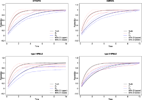
Figure 1: Experiment 1. True cumulative distribution function and the mean of 500 simulations along with 95% confidence band (dotted) for the four proposed estimators. Sample size is 500, censoring rate is 40%.

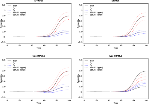
Figure 2: Experiment 2. True cumulative distribution function and the mean of 500 simulations along with 95% confidence band (dotted) for the four proposed estimators. Sample size is 500, censoring rate is 40%.

In contrast, across all experiments and censoring rates, the EM-PAVA estimator performs satisfactorily throughout the entire range of $t$ [see Figures 1, 2 and S.1 (supplementary material)]. The EM-PAVA estimator is as efficient as the Oracle EFFAIPW, but with much smaller bias, especially when censoring is present. The EM-PAVA also performs well in detecting small differences between $F_{1}(t)$ and $F_{2}(t)$. In Table 3, the type I error rates for all estimators adhere to their nominal levels. When $F_{1}(t)$ and $F_{2}(t)$ are largely different (i.e., Experiment 2), then both EM-PAVA and the Oracle EFFAIPW have similar power in detecting differences. However, when $F_{1}(t)$ and $F_{2}(t)$ are different but to a lesser degree (i.e., Experiment 1), then EM-PAVA has larger power in detecting the difference than all other estimators, including the Oracle EFFAIPW. The larger power of the EM-PAVA estimator is not too surprising considering that it estimates ${\mathbf{F}}(t)$ across a range of time points, unlike the pointwise estimation of the Oracle EFFAIPW.

A benefit of EM-PAVA over the Oracle EFFAIPW (and the two NPMLEs) is that EM-PAVA yields a genuine distribution function (i.e., the estimator is monotone, nonnegative and has values in the $[0,1]$ range). The curves shown in Figures 1, 2 and S.1 (supplementary material) for Oracle EFFAIPW are the result of doing a post-estimation procedure to yield monotonicity. The ingenuity of the Oracle EFFAIPW estimator, however, is evident from its 95% confidence band, which was constructed from the 2.5% and 97.5% pointwise quantiles of the 500 Monte Carlo data sets. Figure S.1 (supplementary material) shows that the Oracle EFFAIPW estimator can have 95% confidence bands outside of the $[0,1]$; for large $t$ in Figure S.1, the upper confidence bound is larger than 1. In contrast, the EM-PAVA estimator is always guaranteed to be within $[0,1]$ and, thus, its 95% confidence bands are always within this range.

5 Application to the CORE-PD study

5.1 CORE-PD data and mixture proportions

We applied our estimator to the CORE-PD study introduced in Section 1.1. Data from the CORE-PD study include information from first-degree relatives (i.e., parents, siblings and children) of PARK2 probands. The probands had age at onset (AAO) of Parkinson’s disease (PD) less than or equal to 50 and did not carry mutations in other genes [i.e., neither LRRK2 mutations nor GBA mutations, Marder et al. (2010)]. The key interest is estimating the cumulative risk of PD-onset for the first-degree relatives belonging to different populations: [1.]

PARK2 mutation carrier vs. noncarrier: We compared the estimated cumulative risk in first-degree relatives expected to carrying one or more copies of a mutation in the PARK2 gene (carriers) to relatives expected to carry no mutation (noncarrier).

PARK2 compound heterozygous (or homozygous) mutation carrier vs. heterozygous mutation carrier vs. noncarrier: We considered first-degree relatives who have the compound heterozygous genotype (two or more different copies of the mutation) or homozygous genotype (two or more copies of the same mutation). We compared distribution of risk in this population to two different populations: (a) relatives who are expected to have the heterozygous genotype (mutation on a single allele), and (b) relatives who are expected to be noncarriers (no mutation). These comparisons will bring insight into whether heterozygous PARK2 mutations alone increase the risk of PD or if additional risk alleles play a role.

In the CORE-PD study, the ages at onset for the first-degree relatives are at least 90% censored. Information discerning to which population a relative belongs is available through different mixture proportions. The mixture proportions are vectors $(p_{i},1-p_{i})$, where $p_{i}$ is the probability of the $i$th first-degree relative carrying at least one copy of a mutation. This probability was computed based on the proband’s genotype, a relative’s relationship to a proband under the Mendelian transmission assumption. For example, a child of a heterozygous carrier proband has a probability of 0.5 to inherit the mutated allele, and thus a probability of 0.5 to be a carrier. A child of a homozygous carrier proband has a probability of 1 to be a carrier. More details are given in Wang et al. (2007, 2008). Summary statistics for the populations and the mixture proportions are listed in Table 4.

Table 4: Summary statistics for CORE-PD study. Total number of first-degree relatives ($n$), number of parents, siblings and children, and percentage of first-degree relatives who have the specified mixture proportion $(p,1-p)$, where $p$ is the probability of a relative carrying at least one copy of mutation

					Mixture proportion (%)
	$\bolds{n}$	Parents	Siblings	Children	$\bolds{(1,0)}$	$\bolds{(0,1)}$	$\bolds{(0.5,0.5)}$
Carrier vs. noncarrier	$355$	$63$	$182$	$110$	$31.5$	$64.8$	$3.7$
Compound heterozygous	$17$	$1$	$15$	$1$	$100.0$	$0$	$0$
carrier or homozygous carrier∗
Heterozygous carrier	$338$	$62$	$167$	$109$	$28.1$	$68.1$	$3.8$
vs. noncarrier

[]^∗Genotype for subjects in this group are known.

5.2 Results

We estimated the cumulative risk based on the EM-PAVA estimator and compared its results with the type I NPMLE. The Oracle EFFAIPW estimator could not be used because the high censoring led to unstable estimation: the inverse weights in the estimator were close to zero. Estimates for the PARK2 compound heterozygous (or homozygous) mutation carriers were based on a Kaplan–Meier estimator because these subjects were observed to carry two or more mutations and there is no uncertainty about the relatives’ genotype status (i.e., the data is not mixture data). We report the cumulative risk estimates along with 95% confidence intervals based on 100 Bootstrap replicates.

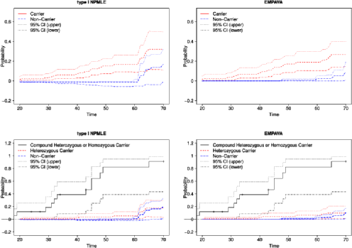
Figure 3: CORE-PD study. Estimated cumulative distribution function for age-at-onset of Parkinson’s disease for Parkin mutation carrier vs. noncarrier (top), and Parkin compound heterozygous or homozygous carrier vs. Parkin heterozygous carrier and noncarrier (bottom).

Figure 3 (top right) shows that by age 50, PARK2 mutation carriers have a large increase in cumulative risk of PD onset compared to noncarriers. Based on EM-PAVA, the cumulative risk (see Table 5) of PD-onset for PARK2 mutation carriers at age 50 is 17.1% (95% CI: 8.5%, 25.6%), whereas the cumulative risk for noncarriers at age 50 is 0.8% (95% CI: 0%, 2.1%). This difference between PARK2 mutation carriers and noncarriers at age 50 was formally tested using the permutation test in Section 3.3. We found that carrying a PARK2 mutation significantly increases the cumulative risk by age 50 ($p$-value${}<0.001$, Table 7), suggesting that a mutation in the PARK2 gene substantially increases the chance of early onset PD. The difference is smaller yet still significant at age 70 ($p\mbox{-value }=0.04$, Table 7). Even across the age range $(20,70)$, the cumulative risk for PARK2 mutation carriers was significantly different than the cumulative risk for noncarriers ($p\mbox{-value }=0.01$0, see Table 7). These findings are consistent with other clinical and biological evidence that PARK2 mutations contribute to early-age onset of PD [Hedrich et al. (2004), Lücking et al. (2000)].

Table 5: Results for Parkin mutation carriers vs. noncarriers: Estimated cumulative distribution function and 95% confidence intervals (in parentheses) based on type I NPMLE and EM-PAVA

	Carrier		Noncarrier
Age	type I NPMLE	EM-PAVA	type I NPMLE	EM-PAVA
20	0.015 (0.000, 0.043)	0.017 (0.000, 0.048)	$-0.011$ ($-0.009$, 0.000)0.	0.000 (0.000, 0.000)
25	0.023 (0.007, 0.061)	0.026 (0.008, 0.068)	$-0.011$ ($-0.013$, $-0.001$)	0.000 (0.000, 0.000)
30	0.032 (0.008, 0.073)	0.036 (0.009, 0.083)	$-0.011$ ($-0.016$, $-0.002$)	0.000 (0.000, 0.000)
35	0.061 (0.026, 0.116)	0.068 (0.029, 0.134)	$-0.011$ ($-0.026$, $-0.007$)	0.000 (0.000, 0.000)
40	0.072 (0.030, 0.128)	0.081 (0.034, 0.143)	$-0.011$ ($-0.030$, $-0.008$)	0.000 (0.000, 0.000)
45	0.121 (0.058, 0.198)	0.137 (0.067, 0.217)	$-0.011$ ($-0.044$, $-0.015$)	0.000 (0.000, 0.000)
50	0.150 (0.074, 0.225)	0.171 (0.085, 0.256)	$-0.011$ ($-0.053$, $-0.005$)	0.008 (0.000, 0.021)
55	0.166 (0.091, 0.263)	0.190 (0.104, 0.299)	$-0.011$ ($-0.057$, $-0.008$)	0.008 (0.000, 0.021)
60	0.166 (0.086, 0.262)	0.190 (0.105, 0.299)	$-0.011$ ($-0.053$, 0.016)0.	0.023 (0.000, 0.053)
65	0.321 (0.117, 0.505)	0.266 (0.138, 0.400)	0.117 ($-0.039$, 0.250)	0.027 (0.000, 0.060)
70	0.321 (0.109, 0.495)	0.266 (0.148, 0.400)	0.170 ($-0.005$, 0.323)	0.094 (0.009, 0.193)

Table 6: Results for Parkin compound heterozygous or homozygous carrier (Compound carrier), Parkin heterozygous carrier and noncarrier: Estimated cumulative distribution function and 95% confidence intervals (in parentheses)

Age	Kaplan–Meier$\bolds{{}^{*}}$		type I NPMLE	EM-PAVA
	Compound carrier		Heterozygous carrier
20	0.118 (0.000, 0.258)		0.000 (0.000, 0.000)0.	0.000 (0.000, 0.000)
25	0.118 (0.000, 0.258)		0.009 (0.000, 0.027)0.	0.010 (0.000, 0.030)
30	0.186 (0.000, 0.355)		0.009 (0.000, 0.027)0.	0.010 (0.000, 0.030)
35	0.389 (0.087, 0.591)		0.009 (0.000, 0.027)0.	0.010 (0.000, 0.030)
40	0.389 (0.087, 0.591)		0.023 (0.000, 0.049)0.	0.026 (0.000, 0.056)
45	0.644 (0.252, 0.830)		0.037 (0.000, 0.089)0.	0.041 (0.000, 0.100)
50	0.822 (0.391, 0.948)		0.037 ($-0.004$, 0.088)	0.041 (0.000, 0.100)
55	0.822 (0.391, 0.948)		0.056 (0.000, 0.119)0.	0.063 (0.000, 0.130)
60	0.822 (0.391, 0.948)		0.056 ($-0.001$, 0.116)	0.064 (0.000, 0.131)
65	0.911 (0.432, 0.986)		0.177 (0.042, 0.304)0.	0.100 (0.016, 0.206)
70	0.911 (0.432, 0.986)		0.177 (0.027, 0.288)0.	0.100 (0.016, 0.206)
			Noncarrier
20			$-0.002$ (0.000, 0.000)0.	0.000 (0.000, 0.000)
25			$-0.002$ ($-0.007$, 0.000)	0.000 (0.000, 0.000)
30			$-0.002$ ($-0.007$, 0.000)	0.000 (0.000, 0.000)
35			$-0.002$ ($-0.007$, 0.000)	0.000 (0.000, 0.000)
40			$-0.002$ ($-0.014$, 0.000)	0.000 (0.000, 0.000)
45			$-0.002$ ($-0.018$, 0.000)	0.000 (0.000, 0.000)
50			$-0.002$ ($-0.015$, 0.014)	0.008 (0.000, 0.022)
55			$-0.002$ ($-0.023$, 0.011)	0.008 (0.000, 0.022)
60			0.0.009 ($-0.022$, 0.044)	0.023 (0.000, 0.055)
65			0.0.142 ($-0.006$, 0.259)	0.032 (0.000, 0.076)
70			0.199 (0.009, 0.334)	0.106 (0.015, 0.181)

[]^∗Genotype for subjects in this group are known. When there is no mixture, both methods reduce to Kaplan–Meier.

To further distinguish the risk of PD among compound heterozygous or homozygous carriers (with at least two copies of mutations) from heterozygous carriers, we separately estimated the distribution functions in these two groups and compared them to the risk in the noncarrier group. The numerical results in Table 6 and a plot of the cumulative risk in Figure 3 (bottom panel) indicate a highly elevated risk in compound heterozygous or homozygous carriers combined. In contrast, the risk for heterozygous carriers closely resembles the risk in noncarriers. This result that being a heterozygous carrier has an essentially similar risk to being a noncarrier was also observed in another study [Wang et al. (2008)]. Further investigation in a larger study is needed to examine whether risk differs in any subgroup. Using a permutation test, we also formally tested for differences between the distribution functions for each group. Results in Table 7 show that there is a significant difference between compound heterozygous carriers and heterozygous carriers as well as a significant difference between compound heterozygous and the noncarriers over the age range $(20,70)$ and at particular ages 50 and 70. Furthermore, there is no significant difference between heterozygous carriers and noncarriers. These analyses suggest a recessive mode of inheritance for PARK2 gene mutations for early-onset PD.

In comparison to the EM-PAVA, the type I NPMLE had wide and nonmonotone confidence intervals, which altered the inference conclusions and is undesirable (see Table 7). Moreover, the type I NPMLE provided a higher cumulative risk in noncarriers by age 70 (17%), which appears to be higher than reported in other epidemiological studies [e.g., Wang et al. (2008)]. The poor performance of the type I NPMLE can be due to instability and inefficiency of the type I, especially at the right-tail area. In contrast, EM-PAVA always provided monotone distribution function estimates, as well as monotone and narrower confidence bands. The EM-PAVA also gave a lower cumulative risk in noncarriers by age 70 (9.4%), which better reflects the population-based estimates. The increased risk in PARK2 carriers at earlier ages compared to population-based estimates can also suggest that there are other genetic and environmental causes of PD in early-onset cases that are different than late onset.

Table 7: $P$-values associated with testing $H_{0}\dvtx F_{1}(t)=F_{2}(t)$ at different $t$-values for CORE-PD study. $H_{0}$ was tested using the permutation test with 1000 permutations

	type I NPMLE	EM-PAVA
	Carrier vs. noncarrier
$t\in[20,70]$	$<$0.013	$<$0.010
$t=50$	$<$0.001	$<$0.001
$t=70$	$<$0.073	.0.04
	Het. carrier vs. noncarrier
$t\in[20,70]$	$<$0.790	$<$0.594
$t=50$	$<$0.341	$<$0.386
$t=70$	$<$0.813	$<$0.969
	Compound het./hom. carrier vs. het. carrier
$t\in[20,70]$	$<$0.013	$<$0.006
$t=50$	$<$0.001	$<$0.001
$t=70$	$<$0.013	$<$0.017
	Compound het/hom. carrier vs. noncarrier
$t\in[20,70]$	$<$0.011	$<$0.007
$t=50$	$<$0.001	$<$0.001
$t=70$	$<$0.013	$<$0.017

6 Concluding remarks

In this work we provide nonparametric estimation of age-specific cumulative risk for mutation carriers and noncarriers. This topic is an important issue in genetic counseling since clinicians and patients use risk estimates to guide their decisions on choices of preventive treatments and planning for the future. For example, individuals with a family history of Parkinson’s disease generally stated that if they were found to be a carrier and in their mid-thirties, they would most likely elect to not have children [McInerney-Leo et al. (2005)]. Or, in the instance they did choose to start a family, PARK2 mutation carriers were more inclined to undergo prenatal testing [McInerney-Leo et al. (2005)].

It is well known that the NPMLE is the most robust and efficient method when there is no parametric assumption for the underlying distribution functions. Unfortunately, in the mixture model discussed in this paper, the NPMLE (type II) fails to produce consistent estimates. On the other hand, the maximum binomial likelihood method studied in this paper provides an alternative consistent estimation method. Moreover, to implement this method, we have used the combination of an EM algorithm and PAVA, which leads to genuine distribution function estimates. For a nonmixture model, the proposed method coincides with the NPMLE. As a result, we expected the proposed method to have high efficiency, which was apparent through the various simulation studies. Even though we only considered two-component mixture models, in principle, the proposed method can be applied to more than two components mixture models without essential difficulty.

In some applications, it may be desirable to consider parametric or semiparametric models (e.g., Cox proportional hazards model, proportional odds model) in a future work. However, diagnosing model misspecification has received little attention in the genetics literature. Our maximum binomial likelihood method can be used as a basis to construct numerical goodness-of-fit tests. In this case, we can test whether the distributions conform to a particular parametric or semiparametric model. That is, the interest is in testing $H_{0}\dvtx F_{1}(t)=F_{1}(t,{\bolds{\beta}}_{1}),F_{2}(t)=F_{2}(t,{\bolds{\beta}}_{2})$ for some parametric models $F_{1}(t,{\bolds{\beta}}_{1})$ and $F_{2}(t,{\bolds{\beta}}_{2})$. To perform this test, we can use the Kolmogorov–Smirnov goodness of fit

$$\Delta=\sqrt{n}\max_{-\infty<t<\infty}\bigl{\{}\bigl{|}\widetilde{F}_{1}(t)-F_{1}(t,\widehat{\bolds{\beta}}_{1})\bigr{|}+\bigl{|}\widetilde{F}_{2}(t)-F_{2}(t,\widehat{\bolds{\beta}}_{2})\bigr{|}\bigr{\}},$$

where $\widehat{\bolds{\beta}}_{1},\widehat{\bolds{\beta}}_{2}$ are the parametric maximum likelihood estimates of ${\bolds{\beta}}_{1}$ and ${\bolds{\beta}}_{2}$. Moreover, if one is interested in estimating other quantities of the underlying distribution functions, for example, the densities, one may use the kernel method to smooth the estimated distribution functions.

In our analysis of CORE-PD data, probands were not included due to concerns of potential ascertainment bias that may be difficult to adjust [Begg (2002)]. In studies where a clear ascertainment scheme is implemented, adjustment can be made based on a retrospective likelihood. Last, the computational procedure of the proposed estimator is simple and efficient. An R function implementing the proposed method is available from the authors.

Appendix: Sketch of technical arguments

.1 The type I and type II NPMLEs

For the type I NPMLE, let $s_{j}(x_{i})={\mathbf{u}}_{j}^{T}{\mathbf{d}}{\mathbf{F}}(x_{i})$ and $S_{j}(x_{i})=1-{\mathbf{u}}_{j}^{T}\,{\mathbf{F}}(x_{i})$, $i=1,\ldots,n$, $j=1,\ldots,m$. The type I NPMLE maximizes

$$\sum_{j=1}^{m}\sum_{i=1}^{n}\log\bigl{\{}s_{j}(x_{i})^{\delta_{i}}S_{j}(x_{i})^{1-\delta_{i}}\bigr{\}}I({\mathbf{q}}_{i}={\mathbf{u}}_{j})$$

with respect to $s_{j}(x_{i})$’s and subject to $\sum_{i=1}^{n}s_{j}(x_{i})I({\mathbf{q}}_{i}={\mathbf{u}}_{j})\leq 1$, $s_{j}(x_{i})\geq 0$ for $j=1,\dots,m$. Because this is equivalent to $m$ separate maximization problems, each concerning $s_{j}(\cdot)$ and $S_{j}(\cdot)$ only, the maximizers are the classical Kaplan–Meier estimators:

$$\widehat{S}_{j}(t)=\prod_{x_{i}\leq t,{\mathbf{q}}_{i}={\mathbf{u}}_{j}}\biggl{\{}1-\frac{\delta_{i}}{\sum_{{\mathbf{q}}_{k}={\mathbf{u}}_{j}}I(x_{k}\geq x_{i})}\biggr{\}},$$

with $s_{j}(t)=S_{j}(t^{-})-S_{j}(t)$ for all $t$. With $\widehat{\mathbf{S}}(t)=\{\widehat{S}_{1}(t),\dots,\widehat{S}_{m}(t)\}^{T}$ and ${\mathbf{U}}=({\mathbf{u}}_{1},\dots,{\mathbf{u}}_{m})^{T}$, the type I NPMLE is

$$\widetilde{\mathbf{F}}_{\mathrm{type\ I}}(t)=\bigl{(}{\mathbf{U}}^{T}{\mathbf{U}}\bigr{)}^{-1}{\mathbf{U}}^{T}\bigl{\{}{\mathbf{1}}_{m}-\widehat{\mathbf{S}}(t)\bigr{\}}.$$

Let the variance–covariance matrix of $\widehat{\mathbf{S}}(t)$ be ${\bolds{\Sigma}}$, which is a diagonal matrix because each of the $m$ components of $\widehat{\mathbf{S}}(t)$ is estimated using a distinct subset of the observations. Then, $\widetilde{\mathbf{F}}_{w}(t)=({\mathbf{U}}^{T}{\bolds{\Sigma}}^{-1}{\mathbf{U}})^{-1}{\mathbf{U}}^{T}{\bolds{\Sigma}}^{-1}\{{\mathbf{1}}_{m}-\widehat{\mathbf{S}}(t)\}$ is a weighted version of the type I NPMLE and is more efficient than the type I NPMLE.

The type II NPMLE has no closed-form solution, and an EM algorithm is typically employed. Specifically, for $k=1,2$, we form at the $b$th step in the EM algorithm

$$c_{ik}^{(b)}=\delta_{i}\frac{q_{ik}\,dF_{k}^{(b)}(x_{i})}{\sum_{k=1}^{2}q_{ik}\,dF_{k}^{(b)}(x_{i})}+(1-\delta_{i})\frac{q_{ik}\{1-F_{k}^{(b)}(x_{i})\}}{\sum_{k=1}^{2}q_{ik}\{1-F_{k}^{(b)}(x_{i})\}},$$

and update the type II NPMLE estimate as

$$1-\check{F}_{{\mathrm{type\ II}},k}^{(b+1)}(t) = \prod_{x_{i}\leq t,\delta_{i}=1}\biggl{\{}1-\frac{\sum_{j=1}^{n}I(x_{j}=x_{i},\delta_{j}=1)c_{jk}^{(b)}}{\sum_{j=1}^{n}c_{jk}^{(b)}I(x_{j}\geq x_{i})}\biggr{\}}$$

$$= \prod_{x_{i}\leq t,\delta_{i}=1}\biggl{\{}1-\frac{c_{ik}^{(b)}}{\sum_{j=1}^{n}c_{jk}^{(b)}I(x_{j}\geq x_{i})}\biggr{\}}.$$

The procedure is iterated until convergence.

.2 Consistency of imputed log-likelihood

We first demonstrate consistency for the noncensored data case. When ${\mathbf{F}}$ takes discrete finite many values, the result holds true trivially. If ${\mathbf{F}}$ is a continuous distribution function, then for noncensored data, the binomial log-likelihood is

$$\ell = \sum_{j=1}^{h}\sum_{i=1}^{n}I(s_{i}\leq t_{j})\log\bigl{[}\lambda_{i}F_{1}(t_{j})+(1-\lambda_{i})F_{2}(t_{j})\bigr{]}$$

$$\quad\qquad{}+I(s_{i}>t_{j})\log\bigl{[}\lambda_{i}\bar{F}_{1}(t_{j})+(1-\lambda_{i})\bar{F}_{2}(t_{j})\bigr{]}.$$

This can be written as

$$n^{-2}\ell = \int\int I(s\leq t)\log\bigl{[}\lambda F_{1}(t)+(1-\lambda)F_{2}(t)\bigr{]}$$

$$\qquad{}+I(s>t)\log\bigl{[}\lambda\bar{F}_{1}(t)+(1-\lambda)\bar{F}_{2}(t)\bigr{]}\,d\eta_{n}(s,\lambda)\,d\xi_{n}(t),$$

where

$$\eta_{n}(s,\lambda)=n^{-1}\sum_{i=1}^{n}I(s_{i}\leq s,\lambda_{i}\leq\lambda),\qquad\xi_{h}(t)=h^{-1}\sum_{i=1}^{h}I(t_{i}\leq t).$$

By the Law of Large Numbers, it can be shown that

$$n^{-2}\ell = \int\bigl{\{}\lambda F_{10}(t)+(1-\lambda)F_{20}(t)\bigr{\}}\log\bigl{\{}\lambda F_{1}(t)+(1-\lambda)F_{2}(t)\bigr{\}}\,d\eta_{0}(\lambda)\,d\xi_{0}(t)$$

$${}+\bigl{\{}\lambda\bar{F}_{10}(t)+(1-\lambda)\bar{F}_{20}(t)\bigr{\}}\log\bigl{\{}\lambda\bar{F}_{1}(t)+(1-\lambda)\bar{F}_{2}(t)\bigr{\}}\,d\eta_{0}(\lambda)\,d\xi_{0}(t)$$

$$=: \Delta,$$

where $\eta_{0}(\lambda)$ is the marginal distribution of $\lambda$ and

$$\xi_{0}(t)=\int\bigl{\{}\lambda F_{10}(t)+(1-\lambda)F_{20}(t)\bigr{\}}\,d\eta_{0}(\lambda).$$

Here, the subscript ₀ denotes the truth. By the Kullback–Leibler information inequality, the above limiting value achieves the maximum if and only if $F_{1}=F_{10}$ and $F_{2}=F_{20}$. Therefore, the maximum binomial likelihood estimation is consistent.

For the censored data case, consistency also holds following a similar argument. The only difference in the log-likelihood is that the indicator function $I(S_{i}\leq t_{j})$ is replaced by $w_{ij}=E\{I(S_{i}\geq t_{j})|S_{i}\geq x_{j}\}$. If $\hat{w}_{i}(t_{j})$ is replaced by an initial consistency estimation, then the log-censored binomial likelihood will converge to $\Delta$ again.

References

- Ayer et al. (1955) {barticle}[mr] \bauthor\bsnmAyer, \bfnmMiriam\binitsM., \bauthor\bsnmBrunk, \bfnmH. D.\binitsH. D., \bauthor\bsnmEwing, \bfnmG. M.\binitsG. M., \bauthor\bsnmReid, \bfnmW. T.\binitsW. T. and \bauthor\bsnmSilverman, \bfnmEdward\binitsE. (\byear1955). \btitleAn empirical distribution function for sampling with incomplete information. \bjournalAnn. Math. Statist. \bvolume26 \bpages641–647. \bidissn=0003-4851, mr=0073895 \bptokimsref\endbibitem
- Barlow et al. (1972) {bbook}[auto:STB—2014/02/12—14:17:21] \bauthor\bsnmBarlow, \bfnmR. E.\binitsR. E., \bauthor\bsnmBartholomew, \bfnmD. J.\binitsD. J., \bauthor\bsnmBremner, \bfnmJ. M.\binitsJ. M. and \bauthor\bsnmBrunk, \bfnmH. D.\binitsH. D. (\byear1972). \btitleStatistical Inference Under Order Restrictions. \bpublisherWiley, \blocationNew York. \bptokimsref\endbibitem
- Begg (2002) {barticle}[pbm] \bauthor\bsnmBegg, \bfnmColin B.\binitsC. B. (\byear2002). \btitleOn the use of familial aggregation in population-based case probands for calculating penetrance. \bjournalJ. Natl. Cancer Inst. \bvolume94 \bpages1221–1226. \bidissn=0027-8874, pmid=12189225 \bptokimsref\endbibitem
- Churchill and Doerge (1994) {barticle}[pbm] \bauthor\bsnmChurchill, \bfnmG. A.\binitsG. A. and \bauthor\bsnmDoerge, \bfnmR. W.\binitsR. W. (\byear1994). \btitleEmpirical threshold values for quantitative trait mapping. \bjournalGenetics \bvolume138 \bpages963–971. \bidissn=0016-6731, pmcid=1206241, pmid=7851788 \bptokimsref\endbibitem
- de Leeuw, Hornik and Mair (2009) {barticle}[auto:STB—2014/02/12—14:17:21] \bauthor\bparticlede \bsnmLeeuw, \bfnmJ.\binitsJ., \bauthor\bsnmHornik, \bfnmK.\binitsK. and \bauthor\bsnmMair, \bfnmP.\binitsP. (\byear2009). \btitleIsotone optimization in R: Pool-adjacent-violators algorithm (PAVA) and active set methods. \bjournalJournal of Statistical Software \bvolume5 \bpages1–24. \bptokimsref\endbibitem
- Efron (1967) {bincollection}[auto:STB—2014/02/12—14:17:21] \bauthor\bsnmEfron, \bfnmB.\binitsB. (\byear1967). \btitleThe two sample problem with censored data. In \bbooktitleProceedings of the Fifth Berkeley Symposium on Mathematical Statistics and Probability, IV \bpages831–853. \bpublisherUniv. California Press, \blocationBerkeley, CA. \bptokimsref\endbibitem
- El Barmi and McKeague (2013) {barticle}[mr] \bauthor\bsnmEl Barmi, \bfnmHammou\binitsH. and \bauthor\bsnmMcKeague, \bfnmIan W.\binitsI. W. (\byear2013). \btitleEmpirical likelihood-based tests for stochastic ordering. \bjournalBernoulli \bvolume19 \bpages295–307. \biddoi=10.3150/11-BEJ393, issn=1350-7265, mr=3019496 \bptokimsref\endbibitem
- Godambe (1960) {barticle}[mr] \bauthor\bsnmGodambe, \bfnmV. P.\binitsV. P. (\byear1960). \btitleAn optimum property of regular maximum likelihood estimation. \bjournalAnn. Math. Statist. \bvolume31 \bpages1208–1211. \bidissn=0003-4851, mr=0123385 \bptokimsref\endbibitem
- Goldwurm et al. (2011) {barticle}[pbm] \bauthor\bsnmGoldwurm, \bfnmStefano\binitsS., \bauthor\bsnmTunesi, \bfnmSara\binitsS., \bauthor\bsnmTesei, \bfnmSilvana\binitsS., \bauthor\bsnmZini, \bfnmMichela\binitsM., \bauthor\bsnmSironi, \bfnmFrancesca\binitsF., \bauthor\bsnmPrimignani, \bfnmPaola\binitsP., \bauthor\bsnmMagnani, \bfnmCorrado\binitsC. and \bauthor\bsnmPezzoli, \bfnmGianni\binitsG. (\byear2011). \btitleKin-cohort analysis of LRRK2-G2019S penetrance in Parkinson’s disease. \bjournalMov. Disord. \bvolume26 \bpages2144–2145. \biddoi=10.1002/mds.23807, issn=1531-8257, pmid=21714003 \bptokimsref\endbibitem
- Grady, Parker-Pope and Belluck (2013) {bmisc}[auto:STB—2014/02/12—14:17:21] \bauthor\bsnmGrady, \bfnmD.\binitsD., \bauthor\bsnmParker-Pope, \bfnmT.\binitsT. and \bauthor\bsnmBelluck, \bfnmP.\binitsP. (\byear2013). \bhowpublishedJolie’s disclosure of preventative mastectomy highlights dilemma. New York Times, May 15, p. A1. \bptokimsref\endbibitem
- Grotzinger and Witzgall (1984) {barticle}[mr] \bauthor\bsnmGrotzinger, \bfnmS. J.\binitsS. J. and \bauthor\bsnmWitzgall, \bfnmC.\binitsC. (\byear1984). \btitleProjections onto order simplexes. \bjournalAppl. Math. Optim. \bvolume12 \bpages247–270. \biddoi=10.1007/BF01449044, issn=0095-4616, mr=0768632 \bptokimsref\endbibitem
- Hedrich et al. (2004) {barticle}[auto:STB—2014/02/12—14:17:21] \bauthor\bsnmHedrich, \bfnmK.\binitsK., \bauthor\bsnmEskelson, \bfnmC.\binitsC., \bauthor\bsnmWilmot, \bfnmB.\binitsB., \bauthor\bsnmMarder, \bfnmK.\binitsK., \bauthor\bsnmHarris, \bfnmJ.\binitsJ., \bauthor\bsnmGarrels, \bfnmJ.\binitsJ., \bauthor\bsnmMeija-Santana, \bfnmH.\binitsH., \bauthor\bsnmVieregge, \bfnmP.\binitsP., \bauthor\bsnmJacobs, \bfnmH.\binitsH., \bauthor\bsnmBressman, \bfnmS. B.\binitsS. B., \bauthor\bsnmLang, \bfnmA. E.\binitsA. E., \bauthor\bsnmKann, \bfnmM.\binitsM., \bauthor\bsnmAbbruzzese, \bfnmG.\binitsG., \bauthor\bsnmMartinelli, \bfnmP.\binitsP., \bauthor\bsnmSchwinger, \bfnmE.\binitsE., \bauthor\bsnmOzelius, \bfnmL. J.\binitsL. J., \bauthor\bsnmPramstaller, \bfnmP. P.\binitsP. P., \bauthor\bsnmKlein, \bfnmC.\binitsC. and \bauthor\bsnmKramer, \bfnmP.\binitsP. (\byear2004). \btitleDistribution, type, and origin of Parkin mutations: Review and case studies. \bjournalMov. Disord. \bvolume19 \bpages1146–1157. \bptokimsref\endbibitem
- Huang, Qin and Zou (2007) {barticle}[mr] \bauthor\bsnmHuang, \bfnmChiung-Yu\binitsC.-Y., \bauthor\bsnmQin, \bfnmJing\binitsJ. and \bauthor\bsnmZou, \bfnmFei\binitsF. (\byear2007). \btitleEmpirical likelihood-based inference for genetic mixture models. \bjournalCanad. J. Statist. \bvolume35 \bpages563–574. \biddoi=10.1002/cjs.5550350407, issn=0319-5724, mr=2416856 \bptokimsref\endbibitem
- Jewell and Kalbfleisch (2004) {barticle}[pbm] \bauthor\bsnmJewell, \bfnmNicholas P.\binitsN. P. and \bauthor\bsnmKalbfleisch, \bfnmJohn D.\binitsJ. D. (\byear2004). \btitleMaximum likelihood estimation of ordered multinomial parameters. \bjournalBiostatistics \bvolume5 \bpages291–306. \biddoi=10.1093/biostatistics/5.2.291, issn=1465-4644, pii=5/2/291, pmid=15054032 \bptokimsref\endbibitem
- Khoury, Beaty and Cohen (1993) {bbook}[auto:STB—2014/02/12—14:17:21] \bauthor\bsnmKhoury, \bfnmM.\binitsM., \bauthor\bsnmBeaty, \bfnmH.\binitsH. and \bauthor\bsnmCohen, \bfnmB.\binitsB. (\byear1993). \btitleFundamentals of Genetic Epidemiology. \bpublisherOxford Univ. Press, \blocationNew York. \bptokimsref\endbibitem
- Kitada et al. (1998) {barticle}[auto:STB—2014/02/12—14:17:21] \bauthor\bsnmKitada, \bfnmT.\binitsT., \bauthor\bsnmAsakawa, \bfnmS.\binitsS., \bauthor\bsnmHattori, \bfnmN.\binitsN., \bauthor\bsnmMatsumine, \bfnmH.\binitsH., \bauthor\bsnmYamamura, \bfnmY.\binitsY., \bauthor\bsnmMinoshima, \bfnmS.\binitsS., \bauthor\bsnmYokochi, \bfnmM.\binitsM., \bauthor\bsnmMizuno, \bfnmY.\binitsY. and \bauthor\bsnmShimizu, \bfnmN.\binitsN. (\byear1998). \btitleMutations in the Parkin gene cause autosomal recessive juvenile parkinsonism. \bjournalNature \bvolume392 \bpages605–608. \bptokimsref\endbibitem
- Kruskal (1964) {barticle}[mr] \bauthor\bsnmKruskal, \bfnmJ. B.\binitsJ. B. (\byear1964). \btitleNonmetric multidimensional scaling: A numerical method. \bjournalPsychometrika \bvolume29 \bpages115–129. \bidissn=0033-3123, mr=0169713 \bptokimsref\endbibitem
- Lücking et al. (2000) {bmisc}[auto:STB—2014/02/12—14:17:21] \bauthor\bsnmLücking, \bfnmC. B.\binitsC. B., \bauthor\bsnmDürr, \bfnmA.\binitsA., \bauthor\bsnmBonifati, \bfnmV.\binitsV., \bauthor\bsnmVaughan, \bfnmJ.\binitsJ., \bauthor\bsnmDe Michele, \bfnmG.\binitsG., \bauthor\bsnmGasser, \bfnmT.\binitsT., \bauthor\bsnmHarhangi, \bfnmB. S.\binitsB. S., \bauthor\bsnmMeco, \bfnmG.\binitsG., \bauthor\bsnmDenefle, \bfnmP.\binitsP., \bauthor\bsnmWood, \bfnmN. W.\binitsN. W., \bauthor\bsnmAgid, \bfnmY.\binitsY., \bauthor\bsnmBrice, \bfnmA.\binitsA., \borganizationFrench Parkinson’s Disease Genetics Study Group and \borganizationEuropean Consortium on Genetic Susceptibility in Parkinson’s Disease (\byear2000). \bhowpublishedAssociation between early-onset Parkinson’s disease and mutations in the Parkin gene. New England Journal of Medicine 342 1560–1567. \bptokimsref\endbibitem
- Luss, Rosset and Shahar (2010) {bmisc}[auto:STB—2014/02/12—14:17:21] \bauthor\bsnmLuss, \bfnmR.\binitsR., \bauthor\bsnmRosset, \bfnmS.\binitsS. and \bauthor\bsnmShahar, \bfnmM.\binitsM. (\byear2010). \bhowpublishedIsotonic recursive partitioning. Preprint. Available at \arxivurlarXiv:1102.5496. \bptokimsref\endbibitem
- Ma and Wang (2012) {barticle}[pbm] \bauthor\bsnmMa, \bfnmYanyuan\binitsY. and \bauthor\bsnmWang, \bfnmYuanjia\binitsY. (\byear2012). \btitleEfficient distribution estimation for data with unobserved sub-population identifiers. \bjournalElectron. J. Stat. \bvolume6 \bpages710–737. \biddoi=10.1214/12-EJS690, issn=1935-7524, mid=NIHMS470955, pmcid=3685883, pmid=23795232 \bptokimsref\endbibitem
- Ma and Wang (2014) {barticle}[auto:STB—2014/02/12—14:17:21] \bauthor\bsnmMa, \bfnmY.\binitsY. and \bauthor\bsnmWang, \bfnmY.\binitsY. (\byear2014). \btitleEstimating disease onset distribution functions in mutation carriers with censored mixture data. \bjournalJ. R. Stat. Soc. Ser. C. Appl. Stat. \bvolume63 \bpages1–23. \bidmr=3148266 \bptokimsref\endbibitem
- Marder et al. (2003) {barticle}[auto:STB—2014/02/12—14:17:21] \bauthor\bsnmMarder, \bfnmK.\binitsK., \bauthor\bsnmLevy, \bfnmG.\binitsG., \bauthor\bsnmLouis, \bfnmE. D.\binitsE. D., \bauthor\bsnmMejia-Santana, \bfnmH.\binitsH., \bauthor\bsnmCote, \bfnmL.\binitsL., \bauthor\bsnmAndrews, \bfnmH.\binitsH., \bauthor\bsnmHarris, \bfnmJ.\binitsJ., \bauthor\bsnmWaters, \bfnmC.\binitsC., \bauthor\bsnmFord, \bfnmB.\binitsB., \bauthor\bsnmFrucht, \bfnmS.\binitsS., \bauthor\bsnmFahn, \bfnmS.\binitsS. and \bauthor\bsnmOttman, \bfnmR.\binitsR. (\byear2003). \btitleAccuracy of family history data on Parkinson’s disease. \bjournalNeurology \bvolume61 \bpages18–23. \bptokimsref\endbibitem
- Marder et al. (2010) {barticle}[pbm] \bauthor\bsnmMarder, \bfnmKaren S.\binitsK. S., \bauthor\bsnmTang, \bfnmMing X.\binitsM. X., \bauthor\bsnmMejia-Santana, \bfnmHelen\binitsH., \bauthor\bsnmRosado, \bfnmLlency\binitsL., \bauthor\bsnmLouis, \bfnmElan D.\binitsE. D., \bauthor\bsnmComella, \bfnmCynthia L.\binitsC. L., \bauthor\bsnmColcher, \bfnmAmy\binitsA., \bauthor\bsnmSiderowf, \bfnmAndrew D.\binitsA. D., \bauthor\bsnmJennings, \bfnmDanna\binitsD., \bauthor\bsnmNance, \bfnmMartha A.\binitsM. A., \bauthor\bsnmBressman, \bfnmSusan\binitsS., \bauthor\bsnmScott, \bfnmWilliam K.\binitsW. K., \bauthor\bsnmTanner, \bfnmCaroline M.\binitsC. M., \bauthor\bsnmMickel, \bfnmSusan F.\binitsS. F., \bauthor\bsnmAndrews, \bfnmHoward F.\binitsH. F., \bauthor\bsnmWaters, \bfnmCheryl\binitsC., \bauthor\bsnmFahn, \bfnmStanley\binitsS., \bauthor\bsnmRoss, \bfnmBarbara M.\binitsB. M., \bauthor\bsnmCote, \bfnmLucien J.\binitsL. J., \bauthor\bsnmFrucht, \bfnmSteven\binitsS., \bauthor\bsnmFord, \bfnmBlair\binitsB., \bauthor\bsnmAlcalay, \bfnmRoy N.\binitsR. N., \bauthor\bsnmRezak, \bfnmMichael\binitsM., \bauthor\bsnmNovak, \bfnmKevin\binitsK., \bauthor\bsnmFriedman, \bfnmJoseph H.\binitsJ. H., \bauthor\bsnmPfeiffer, \bfnmRonald F.\binitsR. F., \bauthor\bsnmMarsh, \bfnmLaura\binitsL., \bauthor\bsnmHiner, \bfnmBrad\binitsB., \bauthor\bsnmNeils, \bfnmGregory D.\binitsG. D., \bauthor\bsnmVerbitsky, \bfnmMiguel\binitsM., \bauthor\bsnmKisselev, \bfnmSergey\binitsS., \bauthor\bsnmCaccappolo, \bfnmElise\binitsE., \bauthor\bsnmOttman, \bfnmRuth\binitsR. and \bauthor\bsnmClark, \bfnmLorraine N.\binitsL. N. (\byear2010). \btitlePredictors of Parkin mutations in early-onset Parkinson disease: The consortium on risk for early-onset Parkinson disease study. \bjournalArch. Neurol. \bvolume67 \bpages731–738. \biddoi=10.1001/archneurol.2010.95, issn=1538-3687, mid=NIHMS368067, pii=67/6/731, pmcid=3329757, pmid=20558392 \bptokimsref\endbibitem
- McInerney-Leo et al. (2005) {barticle}[pbm] \bauthor\bsnmMcInerney-Leo, \bfnmAideen\binitsA., \bauthor\bsnmHadley, \bfnmDonald W.\binitsD. W., \bauthor\bsnmGwinn-Hardy, \bfnmKatrina\binitsK. and \bauthor\bsnmHardy, \bfnmJohn\binitsJ. (\byear2005). \btitleGenetic testing in Parkinson’s disease. \bjournalMov. Disord. \bvolume20 \bpages1–10. \biddoi=10.1002/mds.20316, issn=0885-3185, pmid=15503301 \bptokimsref\endbibitem
- Oliveira et al. (2003) {barticle}[pbm] \bauthor\bsnmOliveira, \bfnmSofia A.\binitsS. A., \bauthor\bsnmScott, \bfnmWilliam K.\binitsW. K., \bauthor\bsnmMartin, \bfnmEden R.\binitsE. R., \bauthor\bsnmNance, \bfnmMartha A.\binitsM. A., \bauthor\bsnmWatts, \bfnmRay L.\binitsR. L., \bauthor\bsnmHubble, \bfnmJean P.\binitsJ. P., \bauthor\bsnmKoller, \bfnmWilliam C.\binitsW. C., \bauthor\bsnmPahwa, \bfnmRajesh\binitsR., \bauthor\bsnmStern, \bfnmMatthew B.\binitsM. B., \bauthor\bsnmHiner, \bfnmBradley C.\binitsB. C., \bauthor\bsnmOndo, \bfnmWilliam G.\binitsW. G., \bauthor\bsnmFred H. Allen, \bfnmJr\binitsJ., \bauthor\bsnmScott, \bfnmBurton L.\binitsB. L., \bauthor\bsnmGoetz, \bfnmChristopher G.\binitsC. G., \bauthor\bsnmSmall, \bfnmGary W.\binitsG. W., \bauthor\bsnmMastaglia, \bfnmFrank\binitsF., \bauthor\bsnmStajich, \bfnmJeffrey M.\binitsJ. M., \bauthor\bsnmZhang, \bfnmFengyu\binitsF., \bauthor\bsnmBooze, \bfnmMichael W.\binitsM. W., \bauthor\bsnmWinn, \bfnmMichelle P.\binitsM. P., \bauthor\bsnmMiddleton, \bfnmLefkos T.\binitsL. T., \bauthor\bsnmHaines, \bfnmJonathan L.\binitsJ. L., \bauthor\bsnmPericak-Vance, \bfnmMargaret A.\binitsM. A. and \bauthor\bsnmVance, \bfnmJeffery M.\binitsJ. M. (\byear2003). \btitleParkin mutations and susceptibility alleles in late-onset Parkinson’s disease. \bjournalAnn. Neurol. \bvolume53 \bpages624–629. \biddoi=10.1002/ana.10524, issn=0364-5134, pmid=12730996 \bptokimsref\endbibitem
- Park, Taylor and Kalbfleisch (2012) {barticle}[mr] \bauthor\bsnmPark, \bfnmYongseok\binitsY., \bauthor\bsnmTaylor, \bfnmJeremy M. G.\binitsJ. M. G. and \bauthor\bsnmKalbfleisch, \bfnmJohn D.\binitsJ. D. (\byear2012). \btitlePointwise nonparametric maximum likelihood estimator of stochastically ordered survivor functions. \bjournalBiometrika \bvolume99 \bpages327–343. \biddoi=10.1093/biomet/ass006, issn=0006-3444, mr=2931257 \bptokimsref\endbibitem
- Qin et al. (2014) {bmisc}[author] \bauthor\bsnmQin, \bfnmJing\binitsJ. \bauthor\bsnmGarcia, \bfnmTanya P.\binitsT. P. \bauthor\bsnmMa, \bfnmYanyuan\binitsY. \bauthor\bsnmTang, \bfnmMing-Xin\binitsM.-X. \bauthor\bsnmMarder, \bfnmKaren\binitsK. and \bauthor\bsnmWang, \bfnmYuanjia\binitsY. (\byear2014). \bhowpublishedSupplement to “Combining isotonic regression and EM algorithm to predict genetic risk under monotonicity constraint.” DOI:\doiurl10.1214/14-AOAS730SUPP. \bptokimsref \endbibitem
- Robertson, Wright and Dykstra (1988) {bbook}[mr] \bauthor\bsnmRobertson, \bfnmTim\binitsT., \bauthor\bsnmWright, \bfnmF. T.\binitsF. T. and \bauthor\bsnmDykstra, \bfnmR. L.\binitsR. L. (\byear1988). \btitleOrder Restricted Statistical Inference. \bpublisherWiley, \blocationChichester. \bidmr=0961262 \bptokimsref\endbibitem
- Struewing et al. (1997) {barticle}[auto:STB—2014/02/12—14:17:21] \bauthor\bsnmStruewing, \bfnmJ. P.\binitsJ. P., \bauthor\bsnmHartge, \bfnmP.\binitsP., \bauthor\bsnmWacholder, \bfnmS.\binitsS., \bauthor\bsnmBaker, \bfnmS. M.\binitsS. M., \bauthor\bsnmBerlin, \bfnmM.\binitsM., \bauthor\bsnmMcAdams, \bfnmM.\binitsM., \bauthor\bsnmTimmerman, \bfnmM. M.\binitsM. M., \bauthor\bsnmBrody, \bfnmL. C.\binitsL. C. and \bauthor\bsnmTuker, \bfnmM. A.\binitsM. A. (\byear1997). \btitleThe risk of cancer associated with specific mutations of BRCA1 and BRCA2 among Ashkenazi Jews. \bjournalNew England Journal of Medicine \bvolume336 \bpages1401–1408. \bptokimsref\endbibitem
- Wang, Garcia and Ma (2012) {barticle}[mr] \bauthor\bsnmWang, \bfnmYuanjia\binitsY., \bauthor\bsnmGarcia, \bfnmTanya P.\binitsT. P. and \bauthor\bsnmMa, \bfnmYanyuan\binitsY. (\byear2012). \btitleNonparametric estimation for censored mixture data with application to the cooperative Huntington’s observational research trial. \bjournalJ. Amer. Statist. Assoc. \bvolume107 \bpages1324–1338. \biddoi=10.1080/01621459.2012.699353, issn=0162-1459, mr=3036398 \bptokimsref\endbibitem
- Wang et al. (2007) {barticle}[auto:STB—2014/02/12—14:17:21] \bauthor\bsnmWang, \bfnmY.\binitsY., \bauthor\bsnmClark, \bfnmL. N.\binitsL. N., \bauthor\bsnmMarder, \bfnmK.\binitsK. and \bauthor\bsnmRobinowitz, \bfnmD.\binitsD. (\byear2007). \btitleNonparametric estimation of genotype-specific age-at-onset distributions from censored kin-cohort data. \bjournalBiometrika \bvolume94 \bpages403–414. \bptokimsref\endbibitem
- Wang et al. (2008) {barticle}[auto:STB—2014/02/12—14:17:21] \bauthor\bsnmWang, \bfnmY.\binitsY., \bauthor\bsnmClark, \bfnmL. N.\binitsL. N., \bauthor\bsnmLouis, \bfnmE. D.\binitsE. D., \bauthor\bsnmMejia-Santana, \bfnmH.\binitsH., \bauthor\bsnmHarris, \bfnmJ.\binitsJ., \bauthor\bsnmCote, \bfnmL. J.\binitsL. J., \bauthor\bsnmWaters, \bfnmC.\binitsC., \bauthor\bsnmAndrews, \bfnmD.\binitsD., \bauthor\bsnmFord, \bfnmB.\binitsB., \bauthor\bsnmFrucht, \bfnmS.\binitsS., \bauthor\bsnmFahn, \bfnmS.\binitsS., \bauthor\bsnmOttman, \bfnmR.\binitsR., \bauthor\bsnmRabinowitz, \bfnmD.\binitsD. and \bauthor\bsnmMarder, \bfnmK.\binitsK. (\byear2008). \btitleRisk of Parkinson’s disease in carriers of Parkin mutations: Estimation using the kin-cohort method. \bjournalArch. Neurol. \bvolume65 \bpages467–474. \bptokimsref\endbibitem
- Wu (1983) {barticle}[mr] \bauthor\bsnmWu, \bfnmC.-F. Jeff\binitsC.-F. J. (\byear1983). \btitleOn the convergence properties of the EM algorithm. \bjournalAnn. Statist. \bvolume11 \bpages95–103. \biddoi=10.1214/aos/1176346060, issn=0090-5364, mr=0684867 \bptokimsref\endbibitem
- Wu, Ma and Casella (2007) {bbook}[mr] \bauthor\bsnmWu, \bfnmRongling\binitsR., \bauthor\bsnmMa, \bfnmChang-Xing\binitsC.-X. and \bauthor\bsnmCasella, \bfnmGeorge\binitsG. (\byear2007). \btitleStatistical Genetics of Quantitative Traits: Linkage, Maps, and QTL. \bpublisherSpringer, \blocationNew York. \bidmr=2344949 \bptokimsref\endbibitem