Analysis of multiple sclerosis lesions via spatially varying coefficients

Abstract

Magnetic resonance imaging (MRI) plays a vital role in the scientific investigation and clinical management of multiple sclerosis. Analyses of binary multiple sclerosis lesion maps are typically “mass univariate” and conducted with standard linear models that are ill suited to the binary nature of the data and ignore the spatial dependence between nearby voxels (volume elements). Smoothing the lesion maps does not entirely eliminate the non-Gaussian nature of the data and requires an arbitrary choice of the smoothing parameter. Here we present a Bayesian spatial model to accurately model binary lesion maps and to determine if there is spatial dependence between lesion location and subject specific covariates such as MS subtype, age, gender, disease duration and disease severity measures. We apply our model to binary lesion maps derived from $T_{2}$-weighted MRI images from 250 multiple sclerosis patients classified into five clinical subtypes, and demonstrate unique modeling and predictive capabilities over existing methods.

, , , and

t1Supported in part by NIH Grant 5-R01-NS-075066-02 (TDJ, TEN), the United Kingdom’s Medical Research Council Grant G0900908 (TEN) and the Wellcome Trust (TEN). The work presented in this manuscript represents the views of the authors and not necessarily that of the NIH, UKMRC or the Wellcome Trust.

1 Introduction

Multiple sclerosis (MS) is an autoimmune disease of the central nervous system characterized by neuronal demyelination that results in brain and spinal cord lesions. These lesions can appear throughout the brain but are more prevalent in white matter. Damage to the myelin and axons, the “wires” of the central nervous system, affects the ability of nerve cells to communicate effectively and leads to deficits in the motor, sensory, visual and autonomic systems [Compston and Coles (2008)]. Clinical symptoms of MS occur in episodic acute periods of attacks (relapsing forms), in gradual progressive deterioration of neurologic function (progressive forms) or in a combination of both [Lublin and Reingold (1996)]. Patients are categorized into different MS subtypes based on these clinical disease courses. However, the progression of the disease and the formation of lesions are highly heterogeneous both within and between individuals.

MRI is an established tool in the diagnosis of MS and in monitoring its evolution [Bakshi et al. (2008), Filippi and Rocca (2011)]. A single MRI scanner can produce a range of different types of images. $T_{1}$-weighted MRI images show white matter as most intense, gray matter darker and cerebral spinal fluid darkest. $T_{2}$-weighted MRI images show cerebral spinal fluid as most intense, gray matter darker and white matter darkest; air has no signal in either type of image. In MS, $T_{1}$-weighted images identify areas of permanent axonal damage that appear as hypointense “black holes.” $T_{2}$-weighted images show both new and old lesions as hyperintense regions. These MRI scans provide complementary information about the nature of MS and are important tools used to monitor disease course in both time and space [Neema et al. (2007)]. $T_{1}$ and $T_{2}$ images also support various approaches in lesion detection, lesion segmentation [Anbeek et al. (2004)], patient phenotyping and patient classification [Bakshi et al. (2008)]. For quantitative analysis of MS lesions from MRI scans, researchers create lesion maps, binary images that mark the exact location of the lesions. After registering all subjects to a common anatomical atlas, they create lesion probability maps (LPM) that show the empirical lesion rate at each voxel (or volume element).

Despite the importance of MRI for management of MS, clinically observed disease progression correlates only poorly with conventional MRI findings; this is so notable that some researchers call the lack of such associations a paradox [Kacar et al. (2011)]. Possible reasons for this paradox include an underestimation of brain damage by conventional MRI and a lack of histopathological specificity of MRI findings [Barkhof (2002)]. This, however, has prompted structural investigations of the so-called normal-appearing brain tissue outside the MR visible lesions [Vrenken et al. (2006)]. For example, another type of MRI, diffusion tensor imaging (DTI), is used for measuring changes in the normal appearing brain tissues [Rovaris et al. (2005)] and is used to investigate the relationship between diffusion abnormalities and clinical disabilities in MS patients [Werring et al. (1999), Filippi et al. (2001), Roosendaal et al. (2009), Goldsmith et al. (2011)].

To better detect and understand MRI-clinical associations, a number of authors have focused on voxel-by-voxel analyses of LPMs. Some studies compare distribution of patterns of lesions from different MS subtypes [Holland et al. (2012), Filli et al. (2012)]. Others have proposed correlating lesion map data with different types of clinical deficits; “Voxel-based lesion-symptom mapping” (VLSM) [Bates et al. (2003)] is the name given to voxel-by-voxel modeling of tissue damage with behavioral and clinical correlates. However, these methods are all “mass univariate” and ignore the spatial dependence between nearby voxels. These methods also use standard linear models that are inappropriate for binary data. Often, researchers smooth the lesion maps, but this does not completely eliminate the non-Gaussian nature of the data and requires an arbitrary choice of the smoothing parameter [Charil et al. (2003, 2007) Kincses et al. (2011), Dalton et al. (2012)]. For example, Charil et al. (2003) perform voxel-wise linear regressions between lesion probability and different clinical disability scores to identify the regions preferentially responsible for different types of clinical deficits. Charil et al. (2007) correlate focal cortical thickness with white matter lesion load and with MS disability scores. In both studies, the authors apply an arbitrary smoothing kernel and perform the analyses independently at each voxel or cortical vertex.

Our motivation for this work is twofold: (1) to appropriately model these binary lesion maps and model the local spatial dependence and, more importantly, (2) to obtain sensitive inferences on the presence of spatial associations between lesion location and subject specific covariates such as MS subtype, age, gender, disease duration (DD) and disease severity as measured by the Expanded Disability Status Scale (EDSS) score and the Paced Auditory Serial Addition Test (PASAT) score. To this end, we propose a Bayesian spatial model of lesion maps. In particular, we propose a spatial generalized linear mixed model with spatially varying coefficients. The spatially varying coefficients are latent spatial processes (or fields). We model these processes jointly using a multivariate pairwise difference prior model, a particular instance of the multivariate conditional autoregressive model [Besag (1974, 1993), Mardia (1988)]. Our model fully respects the binary nature of the data and the spatial structure of the lesion maps as opposed to the aforementioned mass univariate methods. Furthermore, our model produces regularized (smoothed) estimates of lesion incidence without an arbitrary smoothing parameter. Our model also allows for explicit modeling of the spatially varying effects of covariates such as age, gender and disabilities scores (e.g., the EDSS and PASAT scores), producing spatial maps of these effects and their significance, as well as the (scalar) effect of spatially varying covariates such as the fraction of white matter in each voxel.

The idea of spatial modeling with spatially varying coefficient processes traces back to Gelfand et al. (2003). They model the coefficient surface as a realization of a Gaussian spatial process. The correlation function of the Gaussian process determines the smoothness of the process. However, difficulties arise when the number of sites is large. In particular, inversion of the correlation matrix is computationally infeasible. To overcome this difficulty, Banerjee et al. (2008) introduce the Gaussian predictive process. They project the original high-dimensional space onto a low-dimensional subspace with a reduced set of locations, fit a Gaussian process on this subspace and then use Kriging [Krige (1951)] to interpolate back to the original space. Furrer, Genton and Nychka (2006) and Kaufman, Schervish and Nychka (2008) reduce the computational burden by covariance tapering. Covariance tapering is a method whereby the covariance function is attenuated with an appropriate compactly supported positive definite function such that the covariance between pairs of sites that are farther apart than some prespecified constant is set to zero. This results in a sparse covariance matrix that can be inverted using algorithms specifically designed for sparse matrices. A different perspective is to view both the outcome and the coefficient images as 3-dimensional functions, and thus use the framework of functional data analysis [Ramsay and Silverman (2006)]. In particular, function-on-scalar regression models regress functional outcomes on scalar predictors (covariates) [Reiss, Huang and Mennes (2010)]. Reiss and Ogden (2010) propose a functional principle component analysis approach for scalar outcome generalized linear models with functional predictors and spatially varying coefficients. Crainiceanu, Staicu and Di (2009) introduce generalized multilevel functional regression that uses a truncated Karhunen–Loève expansion to estimate spatially varying coefficients. All these alternative approaches rely on data reduction methods or approximations to the processes. In contrast, our model does not rely on data reduction methods or approximations. Parallel computing on a graphical processing unit (GPU) handles the computational burden.

In the next two sections we formulate our Bayesian spatial model and discuss some important algorithmic issues. In Section 4 we apply our model to binary lesion maps derived from $T_{2}$-weighted, high-resolution MRI images from 250 subjects categorized into the five clinical subtypes of MS. We compare our results with a mass univariate logistic regression approach, Firth regression [Firth (1993), Heinze and Schemper (2002)], in terms of both parameter estimates and predictive performance. Results from a simulation study are reported in Section 5. We conclude the paper with a brief discussion. Gibbs sampler details and some theoretical aspects of our model are given in the supplemental article [Ge et al. (2014)].

2 Spatial generalized linear mixed models

Spatial generalized linear mixed models are similar to generalized linear mixed models in that both have a link function, fixed and random components. The difference lies in how both the data and systematic component are functions of space in the former. We have binary data $Y(s)$ for each subject, where $s\in\mathbb{R}^{d}$, for $d\geq 1$ dimensional space (we work exclusively with $d=3$). The link function is a monotonic function that relates the expectation of the random outcome to the systematic component. The systematic component relates a scalar $\eta(s)$ to a linear combination of the covariates: $\eta(s)={\mathbf{x}}^{\mathrm{T}}(s){\bolds\beta}(s)$. That is, the covariates, parameters and $\eta$ are functions of space. This representation of the systematic component is general enough to cover spatially varying coefficients, spatially varying covariates, spatially constant covariates and coefficients, and any combination of the above. Typically for binary data, either the canonical link, the logit link, with the natural parameter, the log odds or the probit link is used. For computational reasons, we use the probit link (see Section 3).

This model, along with appropriate prior distributions for the model parameters, applies to a wide range of scenarios with spatial binary data on a lattice, though we focus only on our neuroimaging application.

2.1 The model

We use notation from the spatial literature and refer to each voxel in the image as a site. Let $s_{j},j=1,\ldots,M$, denote the $j$th site within the brain $\mathcal{B}\subset\mathbb{R}^{3}$, where the sites are ordered lexicographically. For subject $i=1,\ldots,N$ at site $s_{j}$, let $Y_{i}(s_{j})$ denote a Bernoulli random variable representing the presence [$Y_{i}(s_{j})=1$] or absence [$Y_{i}(s_{j})=0$] of a lesion. For subject $i$, let ${\mathbf{x}}_{i}$ denote a column vector of $P$ subject-specific covariates and let $w(s_{j})$ denote a single spatially varying covariate evaluated at site $s_{j}$ that is shared among all subjects. Our spatial generalized linear mixed model at site $s_{j}$ can then be written as

$$\bigl{[}Y_{i}(s_{j})\mid p_{i}(s_{j})\bigr{]} \sim \operatorname{Bernoulli}\bigl{[}p_{i}(s_{j})\bigr{]},$$ (1)

$$\Phi^{-1}\bigl{\{}\mathrm{E}\bigl{[}Y_{i}(s_{j})\mid p_{i}(s_{j})\bigr{]}\bigr{\}} = \eta_{i}(s_{j}),$$ (2)

$$\eta_{i}(s_{j}) = {\mathbf{x}}_{i}^{\mathrm{T}}\bigl{[}\bolds\alpha+\bolds\beta(s_{j})\bigr{]}+w(s_{j}){\gamma},$$ (3)

reflecting the random, link and systematic component, respectively.

The random component is specified in (1), $Y_{i}(s_{j})$ is a Bernoulli random variable where $\Pr[Y_{i}(s_{j})=1]=p_{i}(s_{j})$. The link function is the probit link function, $\Phi^{-1}$, and the systematic component is given by equation (3). The motivation for this specific choice of systematic component will become clear in Section 4. Since the expectation in (2) is equal to the probability that $Y_{i}(s_{j})=1$, $p_{i}(s_{j})$, we can combine these three components into a spatial probit regression model with mixed effects:

$$\Phi^{-1}\bigl{\{}\Pr\bigl{[}Y_{i}(s_{j})=1\mid\eta_{i}(s_{j})\bigr{]}\bigr{\}}={\mathbf{x}}_{i}^{\mathrm{T}}\bigl{[}\bolds\alpha+\bolds\beta(s_{j})\bigr{]}+w(s_{j}){\gamma}.$$ (4)

The fixed effects in this model are the $P$-vector of parameters ${\bolds\alpha}$ and the scalar parameter $\gamma$, while the random effects are the $P$-vectors ${\bolds\beta}(s_{j})$, one at each site. Note that these random effects are spatially varying random effects and not subject specific random effects. Finally, $w(s_{j})$ is a covariate function of space, typically called a spatially varying covariate, while the spatially varying random effects are often called spatially varying coefficients. Note that our model is not implying a causal pathway. Indeed, demyelination, that appears in $T_{2}$-weighted MRI imaging as hyperintense lesions, may cause changes in both EDSS and PASAT. Rather, our model is an association model, relating lesion prevalence to covariates through the spatially varying coefficients.

We conclude our model specification by assigning priors to all parameters. The fixed effect parameters have flat, improper, uninformative priors: $\pi({\bolds\alpha})\propto{\mathbf{1}}$ and $\pi(\gamma)\propto 1$, as is standard for fixed effects regression parameters in Bayesian regression. Spatial parameters have Markov random field or conditional autoregressive model priors to account for the spatial structure. Neighborhood systems of sites define these priors. We regard two sites (i.e., voxels) as neighbors if they share a common face and, thus, a site can have a maximum of six neighbors. If sites $s_{j}$ and $s_{k}$ are neighbors, we write $s_{j}\sim s_{k}$, and we denote the set of neighbors of site $s_{j}$ by $\partial s_{j}=\{s_{k}\dvtx s_{k}\sim s_{j}\}$ and the cardinality of this set by $n(s_{j})$.

The spatial random effect parameters have zero-centered multivariate conditional autoregressive model (MCAR) priors as follows. Define ${\bolds\beta}^{\mathrm{T}}=[{\bolds\beta}^{\mathrm{T}}(s_{1}),\ldots,{\bolds\beta}^{\mathrm{T}}(s_{M})]$: a $\mathrm{PM}$-length column vector. Following the notation in Mardia (1988), the full conditional distribution of ${\bolds\beta}(s_{j})$ is multivariate normal:

$$\bigl{[}{\bolds\beta}(s_{j})\mid{\bolds\beta(-s_{j})},{\bolds\Sigma}\bigr{]}\sim\operatorname{MVN}\biggl{[}\frac{\sum_{s_{r}\in\partial s_{j}}{\bolds\beta}(s_{r})}{n(s_{j})},\frac{{\bolds\Sigma}}{n(s_{j})}\biggr{]},$$ (5)

where ${\bolds\Sigma}$ is a $P\times P$ symmetric positive definite matrix and $\bolds\beta(-s_{j})$ denotes the vector $\bolds\beta$ without the $P$ components at site $s_{j}$. Note here that over most of the interior of the brain $n(s_{j})=6$ and on the surface of the brain $n(s_{j})<6$. Thus, this implies a spatially constant covariance over most of the brain. In the discussion we show how this assumption can be relaxed.

By Brook’s lemma [Brook (1964)], the joint distribution, up to a constant of proportionality, is

$$\pi[{\bolds\beta}\mid{\bolds\Sigma}]\propto\exp\biggl{\{}-\frac{1}{2}\sum_{s_{i}\sim s_{j}}\bigl{[}{\bolds\beta}(s_{i})-{\bolds\beta}(s_{j})\bigr{]}^{\mathrm{T}}{{\bolds\Sigma}}^{-1}\bigl{[}{\bolds\beta}(s_{i})-{\bolds\beta}(s_{j})\bigr{]}\biggr{\}}.$$ (6)

This joint distribution is improper and is not identifiable [Besag (1986)], as we can add an arbitrary constant to ${\bolds\beta}$ without changing the joint distribution. Nevertheless, as long as there is information in the data regarding ${\bolds\beta}$, the posterior of ${\bolds\beta}$ will be proper. Last, we need to place a prior distribution on the hyperprior parameter ${\bolds\Sigma}$ or, equivalently, on the precision matrix ${\bolds\Sigma}^{-1}$. We assign a Wishart prior with $\nu$ degrees of freedom and $P\times P$ identity scale matrix, ${\mathbf{I}}$, to the precision: ${\bolds\Sigma}^{-1}\sim W(\nu,{\mathbf{I}})$. In the analysis below, we assign an improper, uninformative prior to the precision matrix by setting $\nu=0$ while noting that the posterior is proper.

3 Some algorithmic issues

The full conditional posterior distribution of ${\bolds\beta}(s_{j})$ is not easy to sample. We can resort to the Metropolis–Hastings algorithm [Hastings (1970)] or we can introduce continuous latent variables that turn the spatial generalized linear mixed model into a spatial linear mixed model [Albert and Chib (1993)]. We adopt the latter approach, as then all full conditional posterior distributions are easy to sample via Gibbs sampling [Geman and Geman (1984), Gelfand and Smith (1990)]. We begin by introducing $N\times M$ independent continuous normal latent variables $Z_{i}(s_{j}),i=1,\ldots,N$ and $j=1,\ldots,M$, such that

$$\bigl{[}Z_{i}(s_{j})\mid\eta_{i}(s_{j})\bigr{]}\sim\mathrm{N}\bigl{[}\eta_{i}(s_{j}),1\bigr{]}.$$ (7)

Now define the conditional probability that $Y_{i}(s_{j})=1$ given $Z_{i}(s_{j})$ by

$$\Pr\bigl{[}Y_{i}(s_{j})=1\mid Z_{i}(s_{j})\bigr{]}=\cases{1,&\quad$Z_{i}(s_{j})>0,$\vspace*{2pt}\cr 0,&\quad$Z_{i}(s_{j})\leq 0.$}$$

The spatial linear mixed model is now given by (7) and (3) along with the priors specified above. All full conditional posterior distributions are now known distributions that are easy to sample. Thus, the joint posterior of all model parameters, given the latent variables, are updated using a Gibbs sampler.

To show equivalence between the two models (the probit model and the latent variable model), we integrate out the latent variables to recover our probit model (4):

$$\Pr\bigl{[}Y_{i}(s_{j})=1\mid\eta_{i}(s_{j})\bigr{]}$$

$$\qquad=\int_{-\infty}^{+\infty}\Pr\bigl{[}Y_{i}(s_{j})=1\mid z_{i}(s_{j})\bigr{]}\pi\bigl{[}z_{i}(s_{j})\mid\eta_{i}(s_{j})\bigr{]}\,\mathrm{d}z_{i}(s_{j})$$

$$\qquad=1-\Phi\bigl{[}-\eta_{i}(s_{j})\bigr{]}=\Phi\bigl{[}\eta_{i}(s_{j})\bigr{]}.$$

The full conditional distributions of the latent variables are truncated normal distributions:

$$\bigl{[}Z_{i}(s_{j})\mid Y_{i}(s_{j}),\eta_{i}(s_{j})\bigr{]}\sim\cases{\mathrm{N}\bigl{(}\eta_{i}(s_{j}),1\bigr{)}\times I\bigl{(}Z_{i}(s_{j})>0\bigr{)},&\quad$Y_{i}(s_{j})=1,$\vspace*{2pt}\cr\mathrm{N}\bigl{(}\eta_{i}(s_{j}),1\bigr{)}\times I\bigl{(}Z_{i}(s_{j})<0\bigr{)},&\quad$Y_{i}(s_{j})=0,$}$$

where $I(\cdot)$ is the indicator function. We use Robert’s algorithm [Robert (1995)] to efficiently sample these full conditionals. We provide all full conditional posterior distributions in the supplemental article [Ge et al. (2014)].

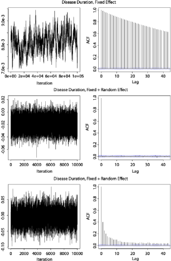
Figure 1: Trace plots and autocorrelation functions (ACFs) for assessing the mixing of our posterior sampler. Top row: Disease duration fixed effect (spatially constant) after the burn-in period, showing extremely strong autocorrelation. Middle and bottom rows: After reparameterizing with sum of fixed and random effects, the autocorrelation is reduced to acceptable levels; middle row shows a voxel with large empirical probability of lesion, while bottom row shows a voxel with an empirical probability of zero. We found similar results for mixed effects estimates at randomly selected locations in the brain.

Another issue is the extremely slow mixing (high autocorrelation) of the fixed effects parameters ${\bolds\alpha}$, as we initially observed and as reported by others [Gelfand et al. (2003)]. We accelerate the mixing by noting that our primary interest is not in the fixed effects, ${\bolds\alpha}$, but rather in the spatially varying coefficients, ${\bolds\alpha}+{\bolds\beta}(s_{j})$. We also note that the posterior variances of the components of ${\bolds\alpha}$ are much smaller than the posterior variances of the components of the ${\bolds\beta}(s_{j})$ and that the ${\bolds\beta}(s_{j})$ do not suffer from slow mixing. Thus, by reparameterizing the model with ${\bolds\beta}^{*}(s_{j})={\bolds\alpha}+{\bolds\beta}(s_{j})$ and placing a nonzero-centered MCAR prior on the ${\bolds\beta}^{*}(s_{j})$, we speed up mixing to acceptable levels (see time series and autocorrelation function plots shown in Figure 1). One can easily recover the marginal posteriors of the components of ${\bolds\alpha}$ by simply taking the average of each component of ${\bolds\beta}^{*}(s_{j})$ over $\mathcal{B}$ during the posterior simulation, that is, at each iteration of the Gibbs sampling algorithm.

The final issue is the sheer size of both data and parameters. In our application data set there are $N=250$ subjects, with $M=274\mbox{,}596$ observed Bernoulli random variables per subject for a total of 68,649,000 observations. The length of each vector ${\bolds\beta}^{*}(s_{j})$ in our application is 10. Thus, the total number of spatially varying coefficients that we need to estimate is 2,745,960 along with the $10\times 10$ covariance matrix ${\bolds\Sigma}$. Therefore, simulating from the full posterior is an onerous task. We reduce this computational burden by coding the problem to run in parallel on a GPU.

We use a NVIDIA Tesla C2050 GPU card that has 3 Gb of main memory and 448 threads (independent processing units). All data and code fit in 522 Mb of memory using floating point memory for real-valued variables. We run the algorithm for 150 thousand iterations, discarding the first 50 thousand as burn-in, at which time the Markov chain has reached its stationary distribution. The algorithm runs in just under 8 hours real time. This is approximately an increase in speed of 45 times: decreasing the real time from 15 days of computing on a single CPU (on a 3 GHz Intel processor, coded in C$++$) to just 8 hours of computing on the GPU.

One trick is necessary when updating the ${\bolds\beta}^{*}(s_{j})$, as they are not independent, creating a problem when parallelizing the code. By leveraging the a priori and a posteriori conditional independence of these vectors, we break the problem into two independent parts. We explain this for the case of a 2-dimensional image, though the extension to 3-dimensions is trivial (and is what we use in practice). The pixels in a 2-dimensional image can be thought of as squares on a checkerboard, alternately colored black and red. Given the first order neighborhood system, the parameters, ${\bolds\beta}^{*}(s_{j})$, on the red squares are conditionally independent given the parameters on the black squares. Similarly, the parameters on the black squares are conditionally independent given the parameters on the red squares. However, neighbors are dependent on one another. Thus, to parallelize this problem, we divide and conquer, by extracting all “black square” parameter vectors and updating them in parallel conditional on the current parameter vector values on the red squares. Likewise, we extract the “red square” parameter vectors and update them in parallel conditional on the current parameter values on the black squares. This divide-and-conquer scheme respects the dependence of neighbors during the parameter updates and, thus, the entire algorithm remains a valid Gibbs updating algorithm.

4 Analysis of MS lesions

Our motivating data set consists of 250 MS patients, each classified into one of five clinical subtypes of MS. In increasing order of clinical severity, these subtypes are clinically isolated syndrome (CIS, 11 subjects), relapsed remitting (RLRM, 173 subjects), primary progressive (PRP, 13 subjects), secondary chronic progressive (SCP, 43 subjects) and primary relapsing (PRL, 10 subjects). We note that CIS is not a true MS subtype, but rather is the first clinical sign that MS may be imminent. Between 30–70% of patients diagnosed with CIS go on to develop MS [Miller et al. (2005), Compston and Coles (2008)]. Lesions were identified on $T_{2}$-weighted images in native resolution, $0.977\times 0.977\times 3.000\ \mathrm{mm}^{3}$. Two neuropathologists independently outline lesions on the MRI scans using a semi-automated approach, and a third radiologist mediates any discrepancies. The result is a binary lesion map with 1 indicating the presence of a lesion and 0 the absence of a lesion at each voxel. The images are then affine registered to the Montreal Neurological Institute (MNI) template at $1\times 1\times 1\ \mathrm{mm}^{3}$ resolution using trilinear interpolation, and thresholded at 0.5 to retain binary values. To reduce the overall size of the images, over 2 million voxels, we subsample every other voxel in each of the $x$-, $y$- and $z$-directions, resulting in binary images with voxel size $2\times 2\times 2\ \mathrm{mm}^{3}$ for a total of $M=274\mbox{,}596$ voxels.

Finally, we note that our model is not dependent on the method of lesion identification and will work with any type of atlas-registered binary image data exhibiting spatial dependence.

In the analysis we use six patient specific covariates: clinical subtype (coded as five dummy variables), age, gender, DD, EDSS score, PASAT score and one spatially varying covariate shared by all subjects, the white matter probability map. The EDSS score is an ordinal measure of overall disability, ranging from zero to ten in increments of one half [Kurtzke (1983)]. The PASAT score is a neuropsychological test that assesses the capacity and rate of information processing as well as sustained and divided attention [Spreen and Strauss (1998)]. We treat clinical subtype as a nominal variable. Subtype classification is based on the clinical course of the disease. Patients classified as RLRM may convert to SCP, but, in general, patients do not progress through the five disease subtypes and, thus, we do not consider subtype as ordinal. The white matter probability map, $w(s_{j})$, is the sole spatially varying covariate. MS is primarily a white matter disease, yet due to imperfect inter-subject registration of the brain images, each subject’s white matter voxels will not perfectly overlap. Thus, instead of constraining our analysis to a set of voxels defining white matter, we choose to analyze all brain voxels and use the white matter spatial covariate to account for the gross differences in lesion incidence over the brain.

Thus, the covariate vector ${\mathbf{x}}_{i}$ has ten components. Associated with each component is a spatially varying coefficient. The first five are the intercepts for the five subtypes, and the remaining are the slopes for age, gender, DD, EDSS score and PASAT score. We do not model interactions between subtypes and covariates, as some subtypes have very little data (e.g., CIS with 11 subjects). We mean-center age, DD, EDSS and PASAT scores prior to the analysis.

4.1 Estimation

We estimate the posterior distribution via Markov chain Monte Carlo (MCMC). In particular, since all full conditional distributions have closed form, we use the Gibbs sampler. We simulate 100,000 draws from the posterior after a burn-in of 50,000, by which time the chain has converged to its stationary distribution, the posterior.

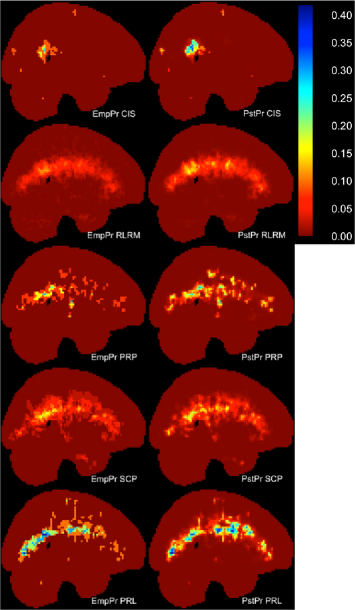
Figure 2: Comparison of the empirical probabilities (left) and the estimated mean posterior probabilities from our model (right) for each of the five MS subtypes. Model estimates exhibit greater smoothness due to our spatial MCAR prior.

Figure 2 (left) shows the empirical lesion probabilities for the five MS subtypes. RLRM and SCP appear to have the most spatially extensive distribution of lesions. This, however, is an artifact of those groups having the most subjects. Figure 2 (right) shows the estimated mean posterior probabilities from our model. Only the CIS patients show a dramatically different spatial distribution of lesion incidence compared to the other subtypes. This likely corresponds to the fact that CIS patients are those first showing signs of having MS and thus have the lowest lesion load. Furthermore, only 11 of the 250 subjects are classified as CIS. However, other subtle differences are evident. For example, PRL patients appear to have the highest overall lesion prevalence.

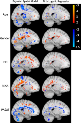
Figure 3: A comparison of thresholded statistical significance maps for covariates. On the left are Bayesian standardized spatial maps (posterior mean divided by posterior standard deviation) for age, gender, disease duration, EDSS and PASAT scores, and on the right are classical statistic spatial maps (mean divided by standard deviation) from the mass univariate Firth logistic regression. Color scale is set from 2 to 5 for positive values (values below 2 are not shown, values of 5 or greater have maximal yellow color), and from $-5$ to $-2$ for negative values (values above $-2$ are not shown, values of $-5$ or smaller have the lightest blue color). The statistic values from Firth logistic regression are significantly attenuated and spatially contracted compared to our model estimates.

Figure 3 is a comparison of the thresholded (at $\pm 2$) statistical maps (spatially varying coefficient estimates divided by their standard deviations) for the covariates. On the left are Bayesian standardized spatial maps (posterior mean divided by posterior standard deviation) for age, gender, DD, EDSS and PASAT scores, and on the right are classical statistic spatial maps (mean divided by standard deviation) from a mass univariate approach using Firth logistic regression [Heinze and Schemper (2002), Firth (1993)]. (Note that we compare with Firth regression as opposed to other published methods [e.g., Kincses et al. (2011)] that use a standard linear model to fit the binary data; as we state in the Introduction, such linear models are inappropriate for binary data.) Firth regression avoids the complete separation problem by shrinking parameter estimates using a penalized likelihood approach. For Firth regression, the mass univariate regressors include the five dummy variables for clinical subtypes: age, gender, DD, EDSS and PASAT scores. Therefore, the Firth regression model shares the same subject specific covariates with our Bayesian spatial model, excluding the white matter spatial regressor, but of course ignores any spatial dependence. (While we could have included the white matter term, each voxel would have a different estimate, whereas it is shared across all voxels in our model.)

Table 1: Proportion of voxels that have standardized coefficients more extreme than $\pm 2$. Our model results in a larger proportion of voxels that are substantially large compared to Firth logistic regression. This is due to the borrowing of strength from neighboring voxels in our model

	Gender	Age	DD	EDSS	PASAT
Bayesian spatial model	3.78%	5.17%	4.73%	4.08%	5.08%
Firth logistic regression	0.75%	1.43%	1.11%	1.80%	1.76%

Firth regression is performed in R with the logistf package (http://cran.r-project.org/web/packages/logistf). In Figure 3, one can see that the standardized parameters from our model are substantially larger and more spatially extensive compared to those from Firth regression. Table 1 numerically contrasts the extent of spatial differences between our model and Firth regression. The scatterplots of standardized parameter estimates in Figure 4 show the strengthening of these estimates. For EDSS, for large positive coefficients, standardized parameter estimates from our spatial model tend to be larger than those from Firth regression. Likewise, for PASAT, both for large positive and negative coefficients, standardized parameter estimates from our model tend to be larger than those from Firth regression. This is a direct consequence of the MCAR prior, allowing parameter estimates from neighboring voxels to borrow strength from one another, producing smaller posterior estimates of the parameter variances. The final result is an increase in standardized parameter estimates and larger spatial extent of the signal.

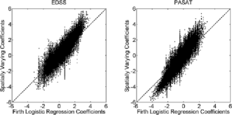
Figure 4: Scatterplots of standardized parameter estimates from our model versus those from Firth logistic regression on a voxel-by-voxel basis. These plots show that statistic estimates from our model tend to have greater magnitude at both large negative and positive values. Vertical streaks reflect how many Firth statistic estimates are the same at different voxels (e.g., where there are no lesions), while our estimates vary. Our model tends to spread out these coefficients due to the spatial smoothing induced by the prior and, to a lesser extent, MCMC error.

We consider age, gender and disease duration as nuisance parameters. Our main interest is in the EDSS and PASAT scores. Figure 5 shows a single sagittal slice of standardized PASAT and EDSS parameter estimates (top left and right, resp.). For reference, the bottom panel shows the reference MRI template (left) and empirical lesion counts overlaid on the reference template (right). PASAT scores are negatively correlated (blue voxels, top left) with lesion occurrence as evident throughout areas of high lesion counts (lower PASAT scores correspond to greater mental deficits). EDSS scores are positively correlated (red voxels, top right) with lesion occurrence within the minor and major forceps (anterior and posterior medial white matter tracks that connect the prefrontal cortex between the two hemispheres of the brain and the parietal/occipital lobes between the two hemispheres, resp.), which is consistent with higher EDSS scores corresponding to more severe MS. To the best of our knowledge, these findings have not been previously reported.

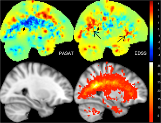
Figure 5: A comparison of statistical significance maps for PASAT and EDSS covariates. A single sagittal slice showing the standardized PASAT and EDSS parameter estimates (top left and right, resp.). High PASAT scores correspond to less damage from MS, and hence negative correlation between PASAT score and lesion occurrence can be seen, especially along the corpus callosum. Higher EDSS scores correspond to more severe MS, and hence the positive correlation between EDSS score and lesion occurrence in the minor and major forceps (anterior and posterior medial white matter tracks, see arrows in the figure) can be seen. For reference, the bottom panel shows the reference $T_{1}$ MRI template (left) and the same with empirical counts overlaid (right).

4.2 Prediction

Using our detailed Bayesian model, it is straightforward to make predictions using Bayes’ theorem. In particular, there is immense potential clinical value in predicting an individual’s MS subtype based on their MRI lesion map, along with their age, gender, DD, EDSS and PASAT scores. To assess the predictive capabilities of our model, we use a cross-validation approach, leaving one subject out at a time. Direct implementation of leave-one-out cross-validation (LOOCV) would be very time consuming, as omitting one subject and rerunning the model would take 8 hours for each of 250 subjects. Thus, we adopt an importance sampling approach originally proposed by Gelfand, Dey and Chang (1992) where we need to run the model only once: We remove each subject’s contribution to the model by adjusting the posterior at each iteration with an importance sample, thus allowing held-out predictions for that subject. We provide details of this importance sampling approach in the supplemental article [Ge et al. (2014)]. We assign, a priori, a categorical distribution to clinical subtype with equal probability of 0.2 to each of the 5 subtypes.

Table 2: The confusion matrices of the LOOCV classification using our Bayesian spatial model (top) based on all in-mask voxels, compared to a Naïve Bayesian classifier (NBC) (middle) and Firth logistic regression (bottom) based on voxels that have at least two lesions across subjects. Equal prior probability is assigned to each subtype when using the Bayesian model. The true subtype is shown in each row and the estimated subtype is shown in each column. The overall and the average classification rates for our Bayesian model are $0.772\pm 0.052$ and $0.828\pm 0.047$, respectively. The overall and the average classification rates for NBC are $0.552\pm 0.062$ and $0.245\pm 0.053$, respectively. The overall and the average classification rates for Firth logistic regression are $0.672\pm 0.058$ and $0.300\pm 0.057$, respectively

	CIS	RLRM	PRP	SCP	PRL
The Bayesian spatial model
CIS	1.000	0.000	0.000	0.000	0.000
RLRM	0.243	0.734	0.000	0.023	0.000
PRP	0.154	0.000	0.846	0.000	0.000
SCP	0.140	0.000	0.000	0.860	0.000
PRL	0.100	0.000	0.100	0.100	0.700
Naïve Bayesian classifier
CIS	0.000	1.000	0.000	0.000	0.000
RLRM	0.046	0.757	0.017	0.093	0.087
PRP	0.077	0.769	0.000	0.077	0.077
SCP	0.023	0.744	0.023	0.070	0.140
PRL	0.000	0.600	0.000	0.000	0.400
Firth logistic regression
CIS	0.000	1.000	0.000	0.000	0.000
RLRM	0.052	0.821	0.006	0.087	0.034
PRP	0.000	0.538	0.000	0.385	0.077
SCP	0.000	0.302	0.023	0.582	0.093
PRL	0.000	0.400	0.000	0.500	0.100

Table 2 (top) shows the LOOCV classification results from our model. The rows show the true clinical subtype, while the columns show our predicted subtype. The overall correct classification rate is $0.772\pm 0.052$ ($X\pm 0.052$ denotes the limits of an approximate 95% confidence interval centered at $X$ based on a normal approximation to a binomial sample proportion). The average classification rate, the unweighted average of the per-subtype correct classification rates, is $0.828\pm 0.047$. Due to the imbalance in group sizes, we find the average classification rate is much more interpretable than the overall correct classification rate. Consider a simple, obviously poor classifier that classifies every one of the 250 subjects as RLRM (when in fact only 173 subjects have this subtype). The overall correct classification rate in this case is $173/250=0.692$, while the average classification rate is $0.2$. The average classification rate balances out extremely high correct classification rates in one or two subtypes that have the largest samples sizes with extremely low correct classification rates in subtypes that have very few subjects. We see in Table 2 (top) that if there is a misclassification, that misclassification tends to be in the CIS subtype. We investigated this further and found that those patients that are misclassified to CIS tend to have fewer and smaller lesions than those correctly classified (see Figure S1 in the supplemental article [Ge et al. (2014)]).

As a comparison, we also perform LOOCV using a naïve Bayesian classifier (NBC) and Firth logistic regression. Both NBC and Firth logistic regression assumes all voxels are mutually independent, ignoring spatial dependence, but NBC bases predictions on the empirical lesion rates alone (see supplemental article [Ge et al. (2014)] for NBC details). While assuming spatial independence seems like a gross oversimplification, empirically NBC often outperforms more sophisticated and computationally expensive approaches [and there are theoretical arguments for this; see Zhang (2004)]. Table 2 (middle and bottom) shows the NBC and Firth regression LOOCV classification results, based on only those voxels that have at least two lesions across all subjects. This ensures that for each voxel, after leaving one subject out, there is at least one lesion in the remaining subjects (classification based on all in-mask voxels produced much worse results). The results of the NBC and Firth regression are largely biased to the RLRM subtype. The overall and the average correct classification rates for the NBC are $0.552\pm 0.062$ and $0.245\pm 0.053$, respectively. The overall and the average correct classification rates for Firth regression are $0.672\pm 0.058$ and $0.300\pm 0.057$, respectively. Despite the theoretical reasons offered by Zhang (2004), for this data set, our modeling approach significantly outperforms NBC in correctly classifying subtype, and it significantly outperforms Firth regression as well.

Although our model tends to misclassify a few patients into the somewhat milder CIS subtype than the other methods, it is much better at correctly classifying patients in the other four subtypes, particularly PRL patients, than the other methods (0.70 versus 0.40 and 0.10; cf. the last entry in each panel). Furthermore, our overall correct and average classification rates are much higher than either the NBC approach or Firth logistic regression. Both of these methods tend to classify most subjects into the RLRM, the subtype with the largest number of patients.

Finally, to confirm that it is the imaging data and not just demographic and clinical variables that are driving prediction, we use a polytomous logistic regression (baseline categories model) with no lesion data to perform this same classification. We found accuracy rates of $0.776\pm 0.052$ (overall) and $0.419\pm 0.061$ (average), demonstrating that it is the imaging data driving prediction accuracy.

4.3 Model diagnostics

As with any regression analyses, model diagnostics should be performed. For binary regression models these include investigation of outlying and influential observations. This should be done for each covariate at each voxel for each subject. However, the sheer size of the problem and data make this untenable. However, careful scrutiny of the coefficient maps, together with estimated mean posterior probability maps, revealed a potential outlier. Figure 6 shows a coronal view of a proton density image (upper left) and the standardized (posterior mean divided by posterior standard deviation) coefficient map (upper right) for age (thresholded at $\pm 2$). The region in question is demarcated by cross-hairs and was identified by its location near the superior cortical gray matter. Although this region has large negative standardized coefficients (voxel at cross-hairs, $-4.3$), the posterior mean coefficient is only $-0.076$ and the mean posterior probability is only $2.5\times 10^{-4}$ (bottom panel). We find that there is one subject with a lesion in this location and she is the second youngest patient in the data set and has no discernible clinical disabilities from her disease. An investigation of her images reveals that there is indeed a lesion located in this region. Thus, although there is strong statistical evidence that younger patients are more likely to have a lesion in this location, there is little scientific significance (an increase in probability of about $2.5\times 10^{-4}$ over a subject one decade older).

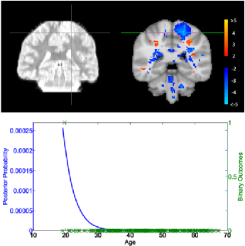
Figure 6: Upper panel: the proton density image (left) of the outlying subject and the standardized age coefficients overlaid on the brain atlas (right). The lesion is seen on the proton density image and the standardized age coefficients (above and below the thresholds, 2 and $-2$, are shown). Lower panel: the fitted posterior lesion probabilities (blue line) as a function of age for a selected voxel (see cross-hairs in upper panel) in “average” RLRM females (gender, disease duration, EDSS and PASAT scores all set to 0). Also shown are the responses for all individuals at the selected voxel.

Each area that may be of interest should be carefully examined, as we have above. This is true for all imaging based models. We therefore caution that the results require careful interpretation along with the empirical and/or posterior probability maps to determine if the results are reliable or are simply the result of an error in marking of a lesion. The area of model diagnostics for large imaging problems is an open problem that requires further work (not only for our model, but for large imaging problems in general), where traditional model diagnostics methods, that rely heavily on graphical outputs, are not feasible.

4.4 Convergence diagnostics

MCMC algorithms must be monitored for convergence. This is typically done by saving the chains for all parameters and assessing convergence either visually or by Markov chain diagnostic methods. Obviously, monitoring the approximately 2.75 million parameters in our model is not feasible. Thus, we selected 10 voxels where we monitor convergence. Some of these voxels are located in regions of high lesion prevalence and others in low lesion prevalence. We ran the model from three random initial parameter settings. Convergence was assessed using the Gelman–Rubin convergence diagnostic for multiple chains [Gelman and Rubin (1992)]. The largest scale reduction factor observed was 1.01, indicating convergence. As another check, we examined the 5 posterior mean coefficient maps of interest (age, gender, disease duration, EDSS and PASAT scores) and searched for the largest difference (in absolute value) between the three possible pairs of runs for each of the 5 coefficient maps. After locating the voxel at which the maximum difference occurs, using the same initial settings and seeds, we reran the 3 simulations, saving the draws of the coefficients at these voxels. Gelman–Rubin convergence diagnostics revealed a largest scale reduction factor of 1.01, indicating convergence at each of these voxels as well.

5 Simulation study

We now present a simulation study to assess our model when ground truth is known. We create 2-dimensional, $100\times 100$, images with different behaviors in each of four $50\times 50$ squares. We assume that there are two groups of subjects consisting of both males and females. The number of lesions in each quadrant is drawn from a Poisson distribution. On average, within the same group, females and males have the same number of lesions on the left two quadrants, while for each quadrant on the right, females have 4 more lesions than males. Similarly, on average, for the same gender, subjects in groups 1 and 2 have the same number of lesions on the top two quadrants, while for each quadrant at the bottom, subjects in group 1 have 4 more lesions than subjects in group 2. The locations of the lesions are uniformly distributed on each quadrant. Each lesion is modeled as a square with side length a random variable uniformly distributed on the set $\{1,3,5\}$. Lesions are allowed to intersect with each other and merge into larger lesions. Figure 7(A) shows the binary images from some randomly selected subjects. For each combination of male vs. female and group 1 vs. group 2, we simulated binary data for ten thousand subjects. With the large number of subjects, an accurate estimation of true lesion probability can be obtained by calculating the empirical lesion rate at each pixel and averaging over each quadrant excluding the outer two edge pixels on all sides to reduce edge effects. For example, the “true” lesion rates for the males in group 1 (the first column in Figure 7) are thus 0.0455, 0.0366, 0.0546 and 0.0459, clockwise, starting with the upper left quadrant.

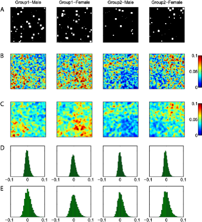
Figure 7: Simulated data results. (A) Lesion patterns from randomly selected subjects. (B) Empirical lesion rates based on 100 randomly generated subjects. (C) Estimated lesion probabilities from the Bayesian spatial model. (D) Histograms of the difference between the estimated probabilities from the Bayesian spatial model and the true probability in the interior area of each quadrant. (E) Histograms of the difference between the estimated probabilities from Firth logistic regression and the true probability in the interior area of each quadrant.

We then randomly selected 100 subjects from each combination, creating a sample size of 400, and fitted our model. The empirical lesion rates from the selected subjects are shown in Figure 7(B). The regressors in the model are gender and two random intercepts corresponding to the two groups. All regressors are associated with spatially varying coefficients. Females are coded 0 and males 1. We consider two pixels to be neighbors if they shared a common edge. The posterior distributions of the parameters are approximated by running the Gibbs sampler for 12,000 iterations, discarding the first 2000 as burn-in. Figure 7(C) shows the estimated lesion probabilities from our Bayesian spatial model. Compared to the empirical rates in Figure 7(B), the smoothing effect is evident. Figure 7(D) shows histograms of the difference between the estimated probabilities from the Bayesian spatial model and the “true” lesion rates in each quadrant. The mean squared error (MSE), averaged over all pixels, is $1.20\times 10^{-4}$. As a comparison, we also performed Firth logistic regression at each pixel. The histograms of the difference between the estimated probabilities from Firth logistic regression and the “true” lesion rates in each quadrant are shown in Figure 7(E). These histograms are wider, and the MSE is $3.33\times 10^{-4}$: approximately 3 times larger.

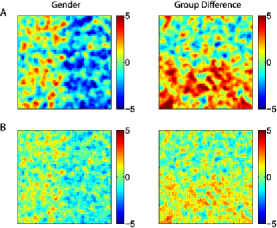
Figure 8: Simulated data results. (A) Standardized spatially varying coefficients of gender and the difference between the two intercepts. (B) Standardized coefficient maps produced by Firth logistic regression.

Figure 8(A) shows the standardized spatially varying coefficients of gender and the difference between the two intercepts (Group1–Group2). The spatial coefficient maps clearly reflect the spatially varying effect of gender and the group difference. Figure 8(B) shows the standardized coefficient maps from Firth logistic regression. Without spatial regularization, the significance map is attenuated relative to that from our model. We note here that the true coefficient maps are not available and that the comparisons made here are relative between the two models.

6 Discussion

In this paper we present a Bayesian spatial model that respects the binary nature of the data and exploits the spatial structure of MS lesion maps without use of an arbitrary smoothing parameter. The method is suitable to model any patterns of lesions, including $T_{2}$ lesions, which show a variety of sizes and shapes, $T_{1}$ “black-hole” lesions and any other types of lesions from which a binary image marking the location of the lesions can be derived. By explicitly including covariates and allowing for spatially varying coefficients, our model provides spatial information that most current empirical approaches cannot; for example, we obtain estimates and estimator precisions for the spatially varying effects of age, gender, DD, EDSS and PASAT.

Our model provides excellent classification accuracy for predicting clinical subtypes of MS based on the entire pattern of lesions over the brain, as well as demographic and behavioral variables. As noted in the Introduction, associations between MRI findings and clinical outcomes have been paradoxically weak. Hence, our construction of a model that not only finds disease subtype differences but also provides high prediction accuracies is an important advance for this area. Specifically, we know of no other work that performs such 5-way classification over disease subtypes. It appears that, by borrowing strength from neighboring voxels and respecting the binary nature of the data, our modeling approach overcomes this paradox to some degree.

Our model is easily extended to include EDSS sub-scores (i.e., disabilities in 7 functional systems) or other diagnostic measures. Last, in Section 2.1 we note that the covariance matrix was constant over much of the brain. This can easily be relaxed by allowing a voxel specific covariance matrix, ${\bolds\Sigma}_{j}$, at the expense of larger computational burden.

The large data set analyzed in this paper, 3-dimensional images each with about 275K voxels from 250 subjects, consists of approximately 70 million observed outcomes, represents a challenge for any spatial data analysis. There are several spatial models, as reviewed in the Introduction, with spatially varying coefficient processes which in principle could be used, but, to our knowledge, have not been applied to such a large problem. Compared to these methods, our model does not require any approximation or data reduction method.

One limitation of our data is the use of affine registration to align subjects to a common space and, thus, a future direction is to use high-dimensional nonlinear registration that can better align brain structures across subjects. We could then investigate whether the predictive accuracy or covariate maps will be improved by the better structural alignment afforded by nonlinear registration. However, an issue with nonlinear registration is that lesion volumes may not change proportionally as they do with affine registration. For a given subject, some lesions may shrink by nonlinear registration while others become larger. When a lesion is shrunk, we are implicitly stating that this lesion is less important for that subject. Thus, an intriguing methodological direction is the development of a model for binary lesion data that accounts for local volume change induced by nonlinear registration, as Voxel Based Morphometry [Ashburner and Friston (2000)] does with its Jacobian-based adjustment.

All code, both CPU and GPU versions, is available by contacting the authors or online at http://go.warwick.ac.uk/tenichols/BSGLMM.

References

- Albert and Chib (1993) {barticle}[mr] \bauthor\bsnmAlbert, \bfnmJames H.\binitsJ. H. and \bauthor\bsnmChib, \bfnmSiddhartha\binitsS. (\byear1993). \btitleBayesian analysis of binary and polychotomous response data. \bjournalJ. Amer. Statist. Assoc. \bvolume88 \bpages669–679. \bidissn=0162-1459, mr=1224394 \bptokimsref\endbibitem
- Anbeek et al. (2004) {barticle}[author] \bauthor\bsnmAnbeek, \bfnmP.\binitsP., \bauthor\bsnmVincken, \bfnmK. L.\binitsK. L., \bauthor\bparticlevan \bsnmOsch, \bfnmM. J. P.\binitsM. J. P., \bauthor\bsnmBisschops, \bfnmR. H. C.\binitsR. H. C. and \bauthor\bsnmvan der Grond, \bfnmJ.\binitsJ. (\byear2004). \btitleProbabilistic segmentation of white matter lesions in MR imaging. \bjournalNeuroImage \bvolume21 \bpages1037–1044. \bptokimsref\endbibitem
- Ashburner and Friston (2000) {barticle}[author] \bauthor\bsnmAshburner, \bfnmJ. T.\binitsJ. T. and \bauthor\bsnmFriston, \bfnmK. J.\binitsK. J. (\byear2000). \btitleVoxel-based morphometry—The methods. \bjournalNeuroImage \bvolume11 \bpages805–821. \bptokimsref\endbibitem
- Bakshi et al. (2008) {barticle}[author] \bauthor\bsnmBakshi, \bfnmR.\binitsR., \bauthor\bsnmThompson, \bfnmA. J.\binitsA. J., \bauthor\bsnmRocca, \bfnmM. A.\binitsM. A., \bauthor\bsnmPelletier, \bfnmD.\binitsD., \bauthor\bsnmDousset, \bfnmV.\binitsV. \betalet al. (\byear2008). \btitleMRI in multiple sclerosis: Current status and future prospects. \bjournalThe Lancet Neurology \bvolume7 \bpages615–625. \bptokimsref\endbibitem
- Banerjee et al. (2008) {barticle}[mr] \bauthor\bsnmBanerjee, \bfnmSudipto\binitsS., \bauthor\bsnmGelfand, \bfnmAlan E.\binitsA. E., \bauthor\bsnmFinley, \bfnmAndrew O.\binitsA. O. and \bauthor\bsnmSang, \bfnmHuiyan\binitsH. (\byear2008). \btitleGaussian predictive process models for large spatial data sets. \bjournalJ. R. Stat. Soc. Ser. B Stat. Methodol. \bvolume70 \bpages825–848. \biddoi=10.1111/j.1467-9868.2008.00663.x, issn=1369-7412, mr=2523906 \bptokimsref\endbibitem
- Barkhof (2002) {barticle}[pbm] \bauthor\bsnmBarkhof, \bfnmFrederik\binitsF. (\byear2002). \btitleThe clinico-radiological paradox in multiple sclerosis revisited. \bjournalCurr. Opin. Neurol. \bvolume15 \bpages239–245. \bidissn=1350-7540, pmid=12045719 \bptokimsref\endbibitem
- Bates et al. (2003) {barticle}[author] \bauthor\bsnmBates, \bfnmE.\binitsE., \bauthor\bsnmWilson, \bfnmS. M.\binitsS. M., \bauthor\bsnmSaygin, \bfnmA. P.\binitsA. P., \bauthor\bsnmDick, \bfnmF.\binitsF., \bauthor\bsnmSereno, \bfnmM. I.\binitsM. I. \betalet al. (\byear2003). \btitleVoxel-based lesion-symptom mapping. \bjournalNature Neuroscience \bvolume6 \bpages448–449. \bptokimsref\endbibitem
- Besag (1974) {barticle}[mr] \bauthor\bsnmBesag, \bfnmJulian\binitsJ. (\byear1974). \btitleSpatial interaction and the statistical analysis of lattice systems. \bjournalJ. R. Stat. Soc. Ser. B Stat. Methodol. \bvolume36 \bpages192–236. \bidissn=0035-9246, mr=0373208 \bptnotecheck related \bptokimsref\endbibitem
- Besag (1986) {barticle}[mr] \bauthor\bsnmBesag, \bfnmJulian\binitsJ. (\byear1986). \btitleOn the statistical analysis of dirty pictures. \bjournalJ. R. Stat. Soc. Ser. B Stat. Methodol. \bvolume48 \bpages259–302. \bidissn=0035-9246, mr=0876840 \bptnotecheck related \bptokimsref\endbibitem
- Besag (1993) {barticle}[author] \bauthor\bsnmBesag, \bfnmJ.\binitsJ. (\byear1993). \btitleTowards Bayesian image analysis. \bjournalJ. Appl. Stat. \bvolume20 \bpages107–119. \bptokimsref\endbibitem
- Brook (1964) {barticle}[mr] \bauthor\bsnmBrook, \bfnmD.\binitsD. (\byear1964). \btitleOn the distinction between the conditional probability and the joint probability approaches in the specification of nearest-neighbour systems. \bjournalBiometrika \bvolume51 \bpages481–483. \bidissn=0006-3444, mr=0205315 \bptokimsref\endbibitem
- Charil et al. (2003) {barticle}[author] \bauthor\bsnmCharil, \bfnmA.\binitsA., \bauthor\bsnmZijdenbos, \bfnmA. P.\binitsA. P., \bauthor\bsnmTaylor, \bfnmJ.\binitsJ., \bauthor\bsnmBoelman, \bfnmC.\binitsC., \bauthor\bsnmWorsley, \bfnmK. J.\binitsK. J. \betalet al. (\byear2003). \btitleStatistical mapping analysis of lesion location and neurological disability in multiple sclerosis: Application to 452 patient data sets. \bjournalNeuroImage \bvolume19 \bpages532–544. \bptokimsref\endbibitem
- Charil et al. (2007) {barticle}[author] \bauthor\bsnmCharil, \bfnmA.\binitsA., \bauthor\bsnmDagher, \bfnmA.\binitsA., \bauthor\bsnmLerch, \bfnmJ. P.\binitsJ. P., \bauthor\bsnmZijdenbos, \bfnmA. P.\binitsA. P., \bauthor\bsnmWorsley, \bfnmK. J.\binitsK. J. \betalet al. (\byear2007). \btitleFocal cortical atrophy in multiple sclerosis: Relation to lesion load and disability. \bjournalNeuroImage \bvolume34 \bpages509–517. \bptokimsref\endbibitem
- Compston and Coles (2008) {barticle}[author] \bauthor\bsnmCompston, \bfnmA.\binitsA. and \bauthor\bsnmColes, \bfnmA.\binitsA. (\byear2008). \btitleMultiple sclerosis. \bjournalThe Lancet \bvolume372 \bpages25–31. \bptokimsref\endbibitem
- Crainiceanu, Staicu and Di (2009) {barticle}[mr] \bauthor\bsnmCrainiceanu, \bfnmCiprian M.\binitsC. M., \bauthor\bsnmStaicu, \bfnmAna-Maria\binitsA.-M. and \bauthor\bsnmDi, \bfnmChong-Zhi\binitsC.-Z. (\byear2009). \btitleGeneralized multilevel functional regression. \bjournalJ. Amer. Statist. Assoc. \bvolume104 \bpages1550–1561. \biddoi=10.1198/jasa.2009.tm08564, issn=0162-1459, mr=2750578 \bptokimsref\endbibitem
- Dalton et al. (2012) {barticle}[author] \bauthor\bsnmDalton, \bfnmC. M.\binitsC. M., \bauthor\bsnmBodini, \bfnmB.\binitsB., \bauthor\bsnmSamson, \bfnmR. S.\binitsR. S., \bauthor\bsnmBattaglini, \bfnmM.\binitsM., \bauthor\bsnmFisniku, \bfnmL. K.\binitsL. K. \betalet al. (\byear2012). \btitleBrain lesion location and clinical status 20 years after a diagnosis of clinically isolated syndrome suggestive of multiple sclerosis. \bjournalMultiple Sclerosis \bvolume18 \bpages322–328. \bptokimsref\endbibitem
- Filippi and Rocca (2011) {barticle}[pbm] \bauthor\bsnmFilippi, \bfnmMassimo\binitsM. and \bauthor\bsnmRocca, \bfnmMaria A.\binitsM. A. (\byear2011). \btitleMR imaging of multiple sclerosis. \bjournalRadiology \bvolume259 \bpages659–681. \biddoi=10.1148/radiol.11101362, issn=1527-1315, pii=259/3/659, pmid=21602503 \bptokimsref\endbibitem
- Filippi et al. (2001) {barticle}[author] \bauthor\bsnmFilippi, \bfnmM.\binitsM., \bauthor\bsnmCercignani, \bfnmM.\binitsM., \bauthor\bsnmInglese, \bfnmM.\binitsM., \bauthor\bsnmHorsfield, \bfnmM. A.\binitsM. A. and \bauthor\bsnmComi, \bfnmG.\binitsG. (\byear2001). \btitleDiffusion tensor magnetic resonance imaging in multiple sclerosis. \bjournalNeurology \bvolume56 \bpages304–311. \bptokimsref\endbibitem
- Filli et al. (2012) {barticle}[author] \bauthor\bsnmFilli, \bfnmL.\binitsL., \bauthor\bsnmHofstetter, \bfnmL.\binitsL., \bauthor\bsnmKuster, \bfnmP.\binitsP., \bauthor\bsnmTraud, \bfnmS.\binitsS., \bauthor\bsnmMueller-Lenke, \bfnmN.\binitsN. \betalet al. (\byear2012). \btitleSpatiotemporal distribution of white matter lesions in relapsing–remitting and secondary progressive multiple sclerosis. \bjournalMultiple Sclerosis Journal \bvolume18 \bpages1577–1584. \bptokimsref\endbibitem
- Firth (1993) {barticle}[mr] \bauthor\bsnmFirth, \bfnmDavid\binitsD. (\byear1993). \btitleBias reduction of maximum likelihood estimates. \bjournalBiometrika \bvolume80 \bpages27–38. \biddoi=10.1093/biomet/80.1.27, issn=0006-3444, mr=1225212 \bptokimsref\endbibitem
- Furrer, Genton and Nychka (2006) {barticle}[mr] \bauthor\bsnmFurrer, \bfnmReinhard\binitsR., \bauthor\bsnmGenton, \bfnmMarc G.\binitsM. G. and \bauthor\bsnmNychka, \bfnmDouglas\binitsD. (\byear2006). \btitleCovariance tapering for interpolation of large spatial datasets. \bjournalJ. Comput. Graph. Statist. \bvolume15 \bpages502–523. \biddoi=10.1198/106186006X132178, issn=1061-8600, mr=2291261 \bptokimsref\endbibitem
- Ge et al. (2014) {bmisc}[author] \bauthor\bsnmGe, \binitsT., \bauthor\bsnmMüller-Lenke, \binitsN., \bauthor\bsnmBendfeldt, \binitsK., \bauthor\bsnmNichols, \binitsT. E. and \bauthor\bsnmJohnson, \binitsT. D. (\byear2014). \bhowpublishedSupplement to “Analysis of multiple sclerosis lesions via spatially varying coefficients.” DOI:\doiurl10.1214/14-AOAS718SUPP. \bptokimsref \endbibitem
- Gelfand, Dey and Chang (1992) {bincollection}[mr] \bauthor\bsnmGelfand, \bfnmA. E.\binitsA. E., \bauthor\bsnmDey, \bfnmD. K.\binitsD. K. and \bauthor\bsnmChang, \bfnmH.\binitsH. (\byear1992). \btitleModel determination using predictive distributions with implementation via sampling-based methods. In \bbooktitleBayesian Statistics, 4 (PeñíScola, 1991) \bpages147–167. \bpublisherOxford Univ. Press, \blocationNew York. \bidmr=1380275 \bptokimsref\endbibitem
- Gelfand and Smith (1990) {barticle}[mr] \bauthor\bsnmGelfand, \bfnmAlan E.\binitsA. E. and \bauthor\bsnmSmith, \bfnmAdrian F. M.\binitsA. F. M. (\byear1990). \btitleSampling-based approaches to calculating marginal densities. \bjournalJ. Amer. Statist. Assoc. \bvolume85 \bpages398–409. \bidissn=0162-1459, mr=1141740 \bptokimsref\endbibitem
- Gelfand et al. (2003) {barticle}[mr] \bauthor\bsnmGelfand, \bfnmAlan E.\binitsA. E., \bauthor\bsnmKim, \bfnmHyon-Jung\binitsH.-J., \bauthor\bsnmSirmans, \bfnmC. F.\binitsC. F. and \bauthor\bsnmBanerjee, \bfnmSudipto\binitsS. (\byear2003). \btitleSpatial modeling with spatially varying coefficient processes. \bjournalJ. Amer. Statist. Assoc. \bvolume98 \bpages387–396. \biddoi=10.1198/016214503000170, issn=0162-1459, mr=1995715 \bptokimsref\endbibitem
- Gelman and Rubin (1992) {barticle}[author] \bauthor\bsnmGelman, \bfnmA.\binitsA. and \bauthor\bsnmRubin, \bfnmD. B.\binitsD. B. (\byear1992). \btitleInference from iterative simulation using multiple sequences. \bjournalStatist. Sci. \bvolume7 \bpages457–472. \bptokimsref\endbibitem
- Geman and Geman (1984) {barticle}[pbm] \bauthor\bsnmGeman, \bfnmS.\binitsS. and \bauthor\bsnmGeman, \bfnmD.\binitsD. (\byear1984). \btitleStochastic relaxation, Gibbs distributions, and the Bayesian restoration of images. \bjournalIEEE Trans. Pattern Anal. Mach. Intell. \bvolume6 \bpages721–741. \bidissn=0162-8828, pmid=22499653 \bptokimsref\endbibitem
- Goldsmith et al. (2011) {barticle}[pbm] \bauthor\bsnmGoldsmith, \bfnmJeff\binitsJ., \bauthor\bsnmCrainiceanu, \bfnmCiprian M.\binitsC. M., \bauthor\bsnmCaffo, \bfnmBrian S.\binitsB. S. and \bauthor\bsnmReich, \bfnmDaniel S.\binitsD. S. (\byear2011). \btitlePenalized functional regression analysis of white-matter tract profiles in multiple sclerosis. \bjournalNeuroimage \bvolume57 \bpages431–439. \biddoi=10.1016/j.neuroimage.2011.04.044, issn=1095-9572, mid=NIHMS294019, pii=S1053-8119(11)00443-5, pmcid=3114268, pmid=21554962 \bptokimsref\endbibitem
- Hastings (1970) {barticle}[author] \bauthor\bsnmHastings, \bfnmW.\binitsW. (\byear1970). \btitleMonte Carlo sampling methods using Markov chains and their applications. \bjournalBiometrika \bvolume57 \bpages97–109. \bptokimsref\endbibitem
- Heinze and Schemper (2002) {barticle}[pbm] \bauthor\bsnmHeinze, \bfnmGeorg\binitsG. and \bauthor\bsnmSchemper, \bfnmMichael\binitsM. (\byear2002). \btitleA solution to the problem of separation in logistic regression. \bjournalStat. Med. \bvolume21 \bpages2409–2419. \biddoi=10.1002/sim.1047, issn=0277-6715, pmid=12210625 \bptokimsref\endbibitem
- Holland et al. (2012) {barticle}[author] \bauthor\bsnmHolland, \bfnmC. M.\binitsC. M., \bauthor\bsnmCharil, \bfnmA.\binitsA., \bauthor\bsnmCsapo, \bfnmI.\binitsI., \bauthor\bsnmLiptak, \bfnmZ.\binitsZ., \bauthor\bsnmIchise, \bfnmM.\binitsM. \betalet al. (\byear2012). \btitleThe relationship between normal cerebral perfusion patterns and white matter lesion distribution in 1249 patients with multiple sclerosis. \bjournalJournal of Neuroimaging \bvolume22 \bpages129–136. \bptokimsref\endbibitem
- Kacar et al. (2011) {barticle}[author] \bauthor\bsnmKacar, \bfnmK.\binitsK., \bauthor\bsnmRocca, \bfnmM.\binitsM., \bauthor\bsnmCopetti, \bfnmM.\binitsM., \bauthor\bsnmSala, \bfnmS.\binitsS., \bauthor\bsnmMesaros, \bfnmS.\binitsS. \betalet al. (\byear2011). \btitleOvercoming the clinical-MR imaging paradox of multiple sclerosis: MR imaging data assessed with a random forest approach. \bjournalAmerican Journal of Neuroradiology \bvolume32 \bpages2098–2102. \bptokimsref\endbibitem
- Kaufman, Schervish and Nychka (2008) {barticle}[mr] \bauthor\bsnmKaufman, \bfnmCari G.\binitsC. G., \bauthor\bsnmSchervish, \bfnmMark J.\binitsM. J. and \bauthor\bsnmNychka, \bfnmDouglas W.\binitsD. W. (\byear2008). \btitleCovariance tapering for likelihood-based estimation in large spatial data sets. \bjournalJ. Amer. Statist. Assoc. \bvolume103 \bpages1545–1555. \biddoi=10.1198/016214508000000959, issn=0162-1459, mr=2504203 \bptokimsref\endbibitem
- Kincses et al. (2011) {barticle}[author] \bauthor\bsnmKincses, \bfnmZ. T.\binitsZ. T., \bauthor\bsnmRopele, \bfnmS.\binitsS., \bauthor\bsnmJenkinson, \bfnmM.\binitsM., \bauthor\bsnmKhalil, \bfnmM.\binitsM., \bauthor\bsnmPetrovic, \bfnmK.\binitsK. \betalet al. (\byear2011). \btitleLesion probability mapping to explain clinical deficits and cognitive performance in multiple sclerosis. \bjournalMultiple Sclerosis Journal \bvolume17 \bpages681–689. \bptokimsref\endbibitem
- Krige (1951) {barticle}[author] \bauthor\bsnmKrige, \bfnmD. G.\binitsD. G. (\byear1951). \btitleA statistical approach to some basic mine valuation problems on the Witwatersrand. \bjournalJournal of Chemical, Metallurgical and Mining Society of South Africa \bvolume52 \bpages119–139. \bptokimsref\endbibitem
- Kurtzke (1983) {barticle}[pbm] \bauthor\bsnmKurtzke, \bfnmJ. F.\binitsJ. F. (\byear1983). \btitleRating neurologic impairment in multiple sclerosis: An expanded disability status scale (EDSS). \bjournalNeurology \bvolume33 \bpages1444–1452. \bidissn=0028-3878, pmid=6685237 \bptokimsref\endbibitem
- Lublin and Reingold (1996) {barticle}[pbm] \bauthor\bsnmLublin, \bfnmF. D.\binitsF. D. and \bauthor\bsnmReingold, \bfnmS. C.\binitsS. C. (\byear1996). \btitleDefining the clinical course of multiple sclerosis: Results of an international survey. National multiple sclerosis society (USA) advisory committee on clinical trials of new agents in multiple sclerosis. \bjournalNeurology \bvolume46 \bpages907–911. \bidissn=0028-3878, pmid=8780061 \bptokimsref\endbibitem
- Mardia (1988) {barticle}[mr] \bauthor\bsnmMardia, \bfnmK. V.\binitsK. V. (\byear1988). \btitleMultidimensional multivariate Gaussian Markov random fields with application to image processing. \bjournalJ. Multivariate Anal. \bvolume24 \bpages265–284. \biddoi=10.1016/0047-259X(88)90040-1, issn=0047-259X, mr=0926357 \bptokimsref\endbibitem
- Miller et al. (2005) {barticle}[author] \bauthor\bsnmMiller, \bfnmD.\binitsD., \bauthor\bsnmBarkhof, \bfnmF.\binitsF., \bauthor\bsnmMontalban, \bfnmX.\binitsX., \bauthor\bsnmThompson, \bfnmA.\binitsA. and \bauthor\bsnmFilippi, \bfnmM.\binitsM. (\byear2005). \btitleClinically isolated syndromes suggestive of multiple sclerosis, part I: Natural history, pathogenesis, diagnosis, and prognosis. \bjournalThe Lancet Neurology \bvolume4 \bpages281–288. \bptokimsref\endbibitem
- Neema et al. (2007) {barticle}[pbm] \bauthor\bsnmNeema, \bfnmMohit\binitsM., \bauthor\bsnmStankiewicz, \bfnmJames\binitsJ., \bauthor\bsnmArora, \bfnmAshish\binitsA., \bauthor\bsnmGuss, \bfnmZachary D.\binitsZ. D. and \bauthor\bsnmBakshi, \bfnmRohit\binitsR. (\byear2007). \btitleMRI in multiple sclerosis: What’s inside the toolbox? \bjournalNeurotherapeutics \bvolume4 \bpages602–617. \biddoi=10.1016/j.nurt.2007.08.001, issn=1933-7213, pii=S1933-7213(07)00146-8, pmid=17920541 \bptokimsref\endbibitem
- Ramsay and Silverman (2006) {bbook}[author] \bauthor\bsnmRamsay, \bfnmJ. O.\binitsJ. O. and \bauthor\bsnmSilverman, \bfnmB. W.\binitsB. W. (\byear2006). \btitleFunctional Data Analysis. \bpublisherWiley. \bptokimsref\endbibitem
- Reiss, Huang and Mennes (2010) {barticle}[mr] \bauthor\bsnmReiss, \bfnmPhilip T.\binitsP. T., \bauthor\bsnmHuang, \bfnmLei\binitsL. and \bauthor\bsnmMennes, \bfnmMaarten\binitsM. (\byear2010). \btitleFast function-on-scalar regression with penalized basis expansions. \bjournalInt. J. Biostat. \bvolume6 \bpages30. \biddoi=10.2202/1557-4679.1246, issn=1557-4679, mr=2683940 \bptokimsref\endbibitem
- Reiss and Ogden (2010) {barticle}[mr] \bauthor\bsnmReiss, \bfnmPhilip T.\binitsP. T. and \bauthor\bsnmOgden, \bfnmR. Todd\binitsR. T. (\byear2010). \btitleFunctional generalized linear models with images as predictors. \bjournalBiometrics \bvolume66 \bpages61–69. \biddoi=10.1111/j.1541-0420.2009.01233.x, issn=0006-341X, mr=2756691 \bptnotecheck year \bptokimsref\endbibitem
- Robert (1995) {barticle}[author] \bauthor\bsnmRobert, \bfnmC. P.\binitsC. P. (\byear1995). \btitleSimulation of truncated normal variables. \bjournalStatist. Comput. \bvolume5 \bpages121–125. \bptokimsref\endbibitem
- Roosendaal et al. (2009) {barticle}[author] \bauthor\bsnmRoosendaal, \bfnmS. D.\binitsS. D., \bauthor\bsnmGeurts, \bfnmJ. J. G.\binitsJ. J. G., \bauthor\bsnmVrenken, \bfnmH.\binitsH., \bauthor\bsnmHulst, \bfnmH. E.\binitsH. E., \bauthor\bsnmCover, \bfnmK. S.\binitsK. S. \betalet al. (\byear2009). \btitleRegional DTI differences in multiple sclerosis patients. \bjournalNeuroImage \bvolume44 \bpages1397–1403. \bptokimsref\endbibitem
- Rovaris et al. (2005) {barticle}[author] \bauthor\bsnmRovaris, \bfnmM.\binitsM., \bauthor\bsnmGass, \bfnmA.\binitsA., \bauthor\bsnmBammer, \bfnmR.\binitsR., \bauthor\bsnmHickman, \bfnmS. J.\binitsS. J., \bauthor\bsnmCiccarelli, \bfnmO.\binitsO. \betalet al. (\byear2005). \btitleDiffusion MRI in multiple sclerosis. \bjournalNeurology \bvolume65 \bpages1526–1532. \bptokimsref\endbibitem
- Spreen and Strauss (1998) {bbook}[author] \bauthor\bsnmSpreen, \bfnmO.\binitsO. and \bauthor\bsnmStrauss, \bfnmE.\binitsE. (\byear1998). \btitleA Compendium of Neuropsychological Tests: Administration, Norms, and Commentary. \bpublisherOxford Univ. Press. \bptokimsref\endbibitem
- Vrenken et al. (2006) {barticle}[author] \bauthor\bsnmVrenken, \bfnmH.\binitsH., \bauthor\bsnmPouwels, \bfnmP. J. W.\binitsP. J. W., \bauthor\bsnmGeurts, \bfnmJ. J. G.\binitsJ. J. G., \bauthor\bsnmKnol, \bfnmD. L.\binitsD. L., \bauthor\bsnmPolman, \bfnmC. H.\binitsC. H. \betalet al. (\byear2006). \btitleAltered diffusion tensor in multiple sclerosis normal-appearing brain tissue: Cortical diffusion changes seem related to clinical deterioration. \bjournalJournal of Magnetic Resonance Imaging \bvolume23 \bpages628–636. \bptokimsref\endbibitem
- Werring et al. (1999) {barticle}[pbm] \bauthor\bsnmWerring, \bfnmD. J.\binitsD. J., \bauthor\bsnmClark, \bfnmC. A.\binitsC. A., \bauthor\bsnmBarker, \bfnmG. J.\binitsG. J., \bauthor\bsnmThompson, \bfnmA. J.\binitsA. J. and \bauthor\bsnmMiller, \bfnmD. H.\binitsD. H. (\byear1999). \btitleDiffusion tensor imaging of lesions and normal-appearing white matter in multiple sclerosis. \bjournalNeurology \bvolume52 \bpages1626–1632. \bidissn=0028-3878, pmid=10331689 \bptokimsref\endbibitem
- Zhang (2004) {binproceedings}[author] \bauthor\bsnmZhang, \bfnmH.\binitsH. (\byear2004). \btitleThe optimality of naive Bayes. In \bbooktitleFLAIRS Conference, \bpublisherUniv. New Brunswick. \bptokimsref\endbibitem