Voxel-level mapping of tracer kinetics in PET studies: A statistical approach emphasizing tissue life tables

Abstract

Most radiotracers used in dynamic positron emission tomography (PET) scanning act in a linear time-invariant fashion so that the measured time-course data are a convolution between the time course of the tracer in the arterial supply and the local tissue impulse response, known as the tissue residue function. In statistical terms the residue is a life table for the transit time of injected radiotracer atoms. The residue provides a description of the tracer kinetic information measurable by a dynamic PET scan. Decomposition of the residue function allows separation of rapid vascular kinetics from slower blood-tissue exchanges and tissue retention. For voxel-level analysis, we propose that residues be modeled by mixtures of nonparametrically derived basis residues obtained by segmentation of the full data volume. Spatial and temporal aspects of diagnostics associated with voxel-level model fitting are emphasized. Illustrative examples, some involving cancer imaging studies, are presented. Data from cerebral PET scanning with ¹⁸F fluoro-deoxyglucose (FDG) and ¹⁵O water (H2O) in normal subjects is used to evaluate the approach. Cross-validation is used to make regional comparisons between residues estimated using adaptive mixture models with more conventional compartmental modeling techniques. Simulations studies are used to theoretically examine mean square error performance and to explore the benefit of voxel-level analysis when the primary interest is a statistical summary of regional kinetics. The work highlights the contribution that multivariate analysis tools and life-table concepts can make in the recovery of local metabolic information from dynamic PET studies, particularly ones in which the assumptions of compartmental-like models, with residues that are sums of exponentials, might not be certain.

abstractwidth280pt

T1Supported in part by the National Institutes of Health (USA) under CA-42045 and by Science Foundation Ireland under 11/PI/1027.

, , , , and

T2Deceased.

1 Introduction

Dynamic PET studies provide the opportunity to image functional metabolic parameters of tissue in-vivo [Phelps (2000)]. Although there have been many developments in this direction [e.g., Cunningham and Jones (1993), Murase (2003), O’Sullivan (1993), Muzi et al. (2012), Veronese et al. (2013)], no procedure has yet been widely adopted for routine use. Most often quantitation of dynamic PET studies is based on consideration of a single time point for a user-defined region of interest (ROI). In view of the complexity of PET imaging and its expense, this is unsatisfactory. As most radiotracers used in PET act in a linear and time-invariant fashion, dynamic PET imaging measures the convolution between the activity of the tracer in the arterial blood supply and the tissue impulse response. The impulse response is known as the tissue residue function. In statistical terms the residue is the life table associated with the collection of PET tracer atoms introduced, typically by intravenous injection, to the circulatory system. The residue has its roots in the seminal indicator dilution work of Meier and Zierler (1954). Kinetic analysis of PET data is substantially concerned with modeling and estimation of the residue function. To this end, there are a suite of commonly used compartmental models [Huang and Phelps (1986)]. However, while compartmental models adequately represent the biochemistry of well-mixed homogeneous in-vitro samples, they are not necessarily well suited to represent micro-vascular flows and micro-heterogeneity that are part of in-vivo tissue [Bassingthwaighte (1970), Li, Yipintsoi and Bassingthwaighte (1997) and Ostergaard et al. (1999)]. Consequently, there is interest in more flexible nonparametric approaches to the estimation of the tissue residues. Among the most popular approaches is the spectral method introduced by Cunningham and Jones (1993). Here residues are approximated by nonnegative sums of exponentials, whose amplitudes and rate constants are adapted to the data; see Veronese et al. (2013) for a recent treatment and review. Spectral methods have the complexity of requiring estimating of a set of intrinsically nonlinear exponential rate constants. This is a significant practical computational challenge; see Zeng et al. (2012), for example. But spectral methods also have a theoretical limitation in that they force the negative-derivative of residue function, aka the transit time density of tracer-atoms, to be monotonically decreasing from a mode at zero. This assumption is at odds with micro-vascular flow measurements which support a more log-Normal or Gamma-like form for the transit time density. If the residue is to be estimated nonparametrically, it is desirable to have a procedure, like that given in Hawe et al. (2012) or O’Sullivan et al. (2009), that does not impose an unrealistic physiologic assumption on the residue function ab initio.

Our focus here is on voxel-level estimation. The method approximates voxel-level residues by a mixture of basis residue functions that have been optimized by applying a backward elimination technique to a segmentation of the entire volume of data. The use of mixtures in this setting is not new [O’Sullivan (1993)], however, unlike the previous work, which has involved approximation of mixtures of compartmental models by a compartmental model form, the current approach does not require this step. An important aspect of the methodology is decomposition of the tissue residue to separately focus on characteristics associated with short transit times of tracer atoms in the vasculature, distinct from slower transit times associated with blood-tissue exchange and retention. This decomposition parallels the often separate consideration given to early and late life-time mortality patterns in human life tables. The methodology leads to a practical quadratic programming-based algorithm for voxel-level residue reconstruction and associated generation of functional metabolic images of parameters of interest. For a typical dynamic PET study the analysis, including the segmentation steps, runs on a 3.2 GHz PC in less than 30 minutes. In the context of PET scanning in cancer applications, that is, about 90% of all clinical PET imaging studies, this is completely adequate for routine operational use.

Section 2 presents the basic statistical models underlying the approach. Inference and model selection methodology are developed in Section 3. Section 4 presents illustrations with imaging data from both normal subjects and cancer patients. Performance of the methodology for ¹⁸F fluoro-deoxyglucose (FDG) and ¹⁵O water (H2O) imaging studies is considered in Section 5. This includes comparisons with compartmental model analysis and more theoretical evaluation via simulations.

2 Theory

Let $C_{T}(t,x)$ represent the concentration of tracer atoms at time $t$ in a tissue voxel with three-dimensional spatial coordinate $x$. $C_{T}(t,x)$, measured as activity per unit mass (mg) of tissue, evolves in response to the localized arterial input function, denoted $C_{P}(t,x)$ and measured as activity per unit volume (ml) of whole blood. The basic assumption of most PET imaging is that the interaction of the tracer with the tissue can be approximated as a linear and time-invariant process. Thus, the measurable concentration arises as a convolution between the tissue response and the arterial input function

$$C_{T}(t,x)=\int_{0}^{t}R(t-s,x)C_{P}(s,x)\,ds.$$ (1)

Here $R(t,x)$ is tissue response and, borrowing terminology of the work of Meier and Zierler (1954) on indicator dilutions, $R(\cdot,x)$ is called the residue function. Formally, $R(\cdot,x)$ is proportional to the impulse response of the tissue at location $x$ and has units of flow (ml$/$g$/$min). If all tracer atoms were instantaneously introduced in a unit volume of blood, $R(\cdot,x)$ would give the number remaining in the tissue as a function of time. If $N$ tracer atoms per ml are introduced in the arterial blood supply to the tissue, for small time increments $\Delta t$, then the number of those atoms, per gram of tissue, remaining in the tissue over the time interval $[t,t+\Delta t]$ is $NR(\cdot,x)\Delta t$. In statistical terms, $R(\cdot,x)$ defines the life table for the time variable which measures the duration of stay of the tracer atom in the tissue—the transit time. Tracer atom transit times are viewed as random—they arise from a range of interactions with an array of micro-vascular flow paths, transporters, enzymes, ligands, etc. that have the potential to influence the overall length of time the tracer atom is in the local tissue region. Measurable transit times are restricted to the observation window $[0,T_{e}]$ of the scanning and, apart from the complexity of indirect measurement by the convolution equation, there is censoring because tracer atoms decay over time. Such restrictions will be familiar, as they arise in traditional life-table work.

2.1 Decomposition of residue and key summary parameters

To better understand the residue, it is helpful to separate the early (vascular) component from the later components that are associated with longer term interaction with the tissue and also retention. Using $\tau_{v}\in(0,T_{e})$ as a cutoff for rapid (large-vessel) transit times, a decomposition of the residue is obtained as

$$R(t,x)=R_{B}(t,x)+R_{D}(t,x)+R_{X}(t,x),$$ (2)

where $R_{B}(t,x)=R(t\land\tau_{v},x)$, $R_{D}(t,x)=R(t\lor\tau_{v},x)-R(T_{e},x)$ and $R_{X}(t,x)$ is the constant $R(T_{e},x)$. We refer to $R_{B}$ as the rapid vascular component, $R_{D}$ as the exchangeable or in-distribution component and $R_{X}$ as the (apparent) extracted component. Apparent is used because the ultimate (asymptotic) extraction is not strictly observable based on the finite duration of the study, however, as it is common to choose $T_{e}$ large enough that there would be little further decline in the residue at times greater than $T_{e}$, $R(T_{e},x)$ should be a good approximation to the relevant flux of the tracer atoms into tissue. The decomposition in (2) is dependent on the value of $\tau_{v}$ (and $T_{e}$). For human imaging, the choice of $\tau_{v}=1$ minute is reasonable, as this matches the early vascular distribution time for intravenously injected contrast agents, upon which the standard scanning duration used to assess local blood volume parameters in computerized tomography (CT) and magnetic resonance (MR) is based [Provenzale et al. (2008)]. In the absence of other information, the temporal resolution of a PET study for the residue can be no better than the temporal sampling of scanning and the sharpness of the arterial input resulting from the intravenous injection of the tracer.

Each component of the residue decomposition in (2) is itself a residue or life table. The extracted component is constant but the vascular and distribution components carry information beyond scale. Key parameters for a residue function are its maximum and integral values, which represent the flow and volume occupied by the collection of tracer atoms defined by the residue [Meier and Zierler (1954), Hawe et al. (2012)]. So based on the decomposition in (2), we identify five summary parameters of particular interest—vascular flow and volume ($K_{B}(x)$, $V_{B}(x)$), distribution flow and volume ($K_{D}(x)$, $V_{D}(x)$) and the apparent flux ($K_{i}(x)$) which is seen as the net flux of tracer into tissue up to time $T_{e}$. A further parameter of interest is the extraction fraction, defined by $\zeta(x)={K_{i}(x)}\cdot{(K_{B}(x)+K_{D}(x)+K_{i}(x))^{-1}}$. In the case where the residue is exponential, for example, a 1-compartment model [e.g., Bassingwaighte (1970)] with rate constants $K_{1}$ and $k_{2}$, for $\tau_{v}=0$, the flow $K_{D}$ reduces to $K_{1}$ and as $T_{e}\rightarrow\infty$ the exchangeable volume $V_{D}\rightarrow\frac{K_{1}}{k_{2}}$. Also, for a 2-compartment FDG model [Phelps et al. (1979)] with $k_{4}=0$ and $\tau_{v}=0$, as $T_{e}\rightarrow\infty$ $K_{D}\rightarrow\frac{K_{1}k_{2}}{k_{2}+k_{3}}$, $V_{D}\rightarrow\frac{K_{D}}{k_{2}+k_{3}}$ and the flux value $K_{i}(x)\rightarrow\frac{K_{1}k_{3}}{k_{2}+k_{3}}$.

Substitution of the residue decomposition (2) into (1) gives a decomposition of the tracer tissue concentration as a sum of vascular ($C_{V}$), in distribution ($C_{D}$) and extracted ($C_{X}$) components

$$C_{T}(t,x)=C_{V}(t,x)+C_{D}(t,x)+C_{X}(t,x).$$ (3)

The sum $C_{E}(t,x)=C_{D}(t,x)+C_{X}(t,x)$ is the extravascular component. Examples of this are shown in Section 4. As $R_{X}$ is constant, $C_{X}(t,x)$ is the product of flux and the cumulative arterial activity. At late time points, vascular and exchangeable concentration are safely ignored so the late time concentration is effectively proportional to the cumulative arterial activity. This is the basis of a model-free approach to the analysis of flux [Patlak, Blasberg and Fenstermacher (1983)].

2.2 Additive modeling of the tissue residue

A variety of blood-tissue exchange models, for example, Bassingwaighte (2000), Huang and Phelps (1986) and Gunn et al. (2002), as well as many general life-table methods, for example, Cox and Oakes (2001) and Lawless (2003), might be used to approximate tissue residue functions. We should allow any approach that does not systematically misrepresent the physiologic/metabolic processes involved. Validation of model formulations for PET tracers is difficult. In-vitro studies clarify important biochemical transformations involved, but satisfactory in-vivo validation of model assumptions related to the structure of micro-vasculature flows and heterogeneities is not possible. The most widely used one- and two-compartment models in PET reduce to representation of the residue by sums of mono-exponential functions. While these models may adequately represent the biochemistry involved, their ability to describe the complexities of vascular transport is limited. Indeed, in the standard compartmental models the tracer atom transit time density is always monotonically decreasing, so the modal transit time for the nonextracted tracer is always zero. Physiologically this is difficult to justify [Bassingwaighte (1970)].

We use an additive model that approximates the local tissue residue by a positive linear sum of a fixed set of distinct basis residue functions, $\bar{R}_{1},\bar{R}_{2},\ldots,\bar{R}_{J}$, that have themselves been derived from a nonparametric analysis of time courses arising from a full segmentation of the data volume. The model is

$$R(t,x)\approx\alpha_{1}(x)\bar{R}_{1}(t)+\alpha_{2}(x)\bar{R}_{2}(t)+\cdots+\alpha_{J}(x)\bar{R}_{J}(t),$$ (4)

where the $\alpha_{j}$’s are nonnegative constants. For simplicity, the basis residues are normalized to have maximum of unity, that is, $\bar{R}_{j}(0)=1$ for $j=1,2,\ldots,J$. Assuming $C_{P}(t,x)$ can be described by a delayed version of a sampled arterial time-course $C_{P}(t)$, which, in view of the temporal resolution of PET, is reasonable, equation (4) implies

$$C_{T}(t,x) = \alpha_{1}(x)\bar{C}_{1}\bigl{(}t-\Delta(x)\bigr{)}+\alpha_{2}(x)\bar{C}_{2}\bigl{(}t-\Delta(x)\bigr{)}+\cdots$$

$${}+\alpha_{J}(x)\bar{C}_{J}\bigl{(}t-\Delta(x)\bigr{)},$$

where $\bar{C}_{j}(t)=\int_{0}^{t}\bar{R}_{j}(t-s)C_{P}(s)\,ds$ for $j=1,2,\ldots,J$. For known delay, $\Delta(x)$, the model is linear in the $\alpha$-coefficients. Note estimation of the $\alpha$’s in (2.2) allows the local residues to be determined by equation (4); from them associated flow and volume parameters of Section 2.1 can be recovered.

Remarks

1. If the $\bar{C}_{j}$’s in (2.2) correspond to specific regional time courses, a mixture model interpretation for the model can be developed. This is reasonable, as the population of available metabolic pathways for a tracer atom is determined by the profile of enzymes, receptor ligands or transporters that are represented. Across a collection of voxels these profiles vary with a greater representation of certain characteristics in some voxels than in others. Thus, the transit time for a randomly chosen tracer atom in voxel $x$ can be expected to select a metabolic pathway in accordance with the distribution of pathways available within the voxel, and the $\alpha$-coefficients (scaled to sum to unity) could be viewed as a set of mixing proportions; see O’Sullivan (1993, 2006). The form in equation (4) can also be viewed as an example of a general multivariate factor analysis (without reference to residues). Such models have been used to describe PET time-course data; see, for example, Kassinen et al. (2005), Layfield and Venegas (2005), Lee et al. (2005) and Zhou et al. (2002).

2. A tissue region can contain significant nonarterial blood vessels. Depending on tissue location, separate signals associated with major blood pools in the circulatory system, such as the right ventricle of the heart, the lungs, venous blood and the venous supply path from the injection site to the heart, might need to be considered. This can be accomplished by augmenting equation (2.2) to include terms representing nonarterial blood signals. Obviously this is particularly relevant in the thoracic imaging where the direct or indirect (via a spillover artifact) impact of nonarterial cardiac and pulmonary blood signals can be significant. Venous blood vessels arise throughout the body, so there is a case for always including a venous signal term. But rarely does the simultaneous measurement of arterial and venous blood activity arise in a PET study. Venous blood can be viewed as a response to the arterial supply, so the venous signal is sensibly represented as a whole-body response to the arterial supply—$C_{V}(t)=\int_{0}^{t}R_{V}(t-s)C_{P}(s)\,ds$. Thus, if an explicit venous signal is not available, the structure of our modeling approach allows for the component $R_{j}$-residues to adapt to $R_{V}$ so that the overall tissue residue will have the venous component included. As mean transit times from arterial to venous blood are short ($<$1 minute), our proposed decomposition of the residue with $\tau_{b}<1$ will be a combination of pure arterial, venous contributions. Hence, $V_{B}(x)$ should be viewed as an estimate of the volume (per mg) of large arterial and large venous vessels in the tissue. Thus, if an explicit venous blood signal is included ($\alpha_{0}(x)C_{V}(t-\Delta(x))$), the local estimate of blood volume should be the sum of the venous volume [i.e., $\alpha_{0}(x)$] and $V_{B}(x)$ from the estimated residue in (2).

3. Due to limited resolution, voxel-level data are subject to mixing and partial volume effects, which are reasonably modeled by mixtures; see also Section 3.3.

3 Inference techniques

The estimation of voxel-level residues involves three steps. First, a segmentation procedure is applied to extract scaled time-course patterns from the measured set of voxel-level time courses in the data. Next, the time courses are analyzed to recover a nonparametric residue function for each and a backward elimination procedure is used to obtain a reduced set of basis residue functions. The final step does voxel-level optimization of $\alpha$-coefficients and delay in equation (2.2) with subsequent evaluation of the voxel residue in equation (4) and the key parameters identified in Section 2.1. The details involved in each of these steps are presented below. As the analysis is based on a voxel-level fitting process, the residuals associated with the fitting process provide useful diagnostic information. Some proposals for examining the temporal and spatial patterns in those residuals are indicated.

3.1 Segmentation

A split-and-merge segmentation procedure fromO’Sullivan (2006) is used. The procedure groups voxels on the basis of the shape of the measured time course, the scaled time course. The splitting employs a principal component analysis to recursively divide the tissue volume into a large collection (typically 10,000) of hyper-rectangular regions whose scaled time-course patterns show maximal homogeneity. The merging process then recursively combines (initially with a constraint to ensure that segments consist of contiguous collections of voxels) these regions to create a collection of regions with high average within-region homogeneity. For the analyses reported here, the number of segments used is taken to be large enough to explain 95% of the variance in the scaled time-course data, about 7–12 segments for a typical cerebral study and 15–20 segments for a chest or abdominal study. The choice of the number of segments was examined in O’Sullivan (2006). As the focus of the algorithm is on scaled time-course information, the extracted segments are well suited for use in subsequent mixture modeling. A particular advantage of the scaled approach is that it results in fewer segments than might otherwise be required to explain a comparable proportion of variance in the data. It is helpful to display segments to connect with anatomy. If the average scaled time course for a segment is given by a vector $\mu$, imaging the $\mu$-weighted average of the voxel-level time-course data in the segment is effective. Some examples are shown in Section 4.

3.2 Construction of basis residues

The time bins of data acquisition are $[$ṯ${}_{b},\bar{t}_{b})$ for $b=1,2,\ldots,B$. The segmentation algorithm provides a mean time course and associated sample variance vector, $\{(y_{kb},v_{kb})$ for $b=1,2,\ldots,B\}$, for each of $k=1,2,\ldots,K$ segments. Arising from the underlying Poisson emissions that are the basis of the imaging process, regional time-course data have an approximate quasi-Poisson structure [see Huesman (1984); Carson et al. (1993) and Hawe et al. (2012)], that is,

$$\mathrm{E}(y_{kb})=\mu_{kb}\quad\mbox{and}\quad\mathrm{V}(y_{kb})\approx\phi_{k}\mu_{kb}$$ (6)

for $\phi_{k}>1$. Thus, up to known calibration factors (incorporating time-bin duration and voxel dimension), the mean values are proportional to the integrated concentration per milligram of radioactive tracer atoms which in turn is a function of the regional residue $R_{k}$ and input arterial supply:

$$\mu_{kb}=\int_{\underline{t}_{b}}^{{\bar{t}}_{b}}C_{k}(t)e^{-\lambda t}\,dt\quad\mbox{and}\quad C_{k}(t)=\int_{0}^{t}R_{k}(t-s)C_{P}(s-\Delta_{k})\,ds,$$ (7)

where $\lambda$ represents isotope decay and $\Delta_{k}$ is an appropriate delay. Note $C_{k}(t)$ here represents the total (radioactive and nonradioactive) tracer atom concentration at time $t$. An initial set of possible residue basis elements are obtained by representation of the $R_{k}$’s in terms of B-splines [O’Sullivan et al. (2009)]. Here the B-spline coefficients and the delay $\Delta_{k}$ are optimized by weighted least squares with weights $\varpi_{kb}$ given by $v_{kb}^{-1}$.

We seek to express the segment residues in terms of a reduced set of basis residue forms. Since retention is apparent in nearly all residues, it makes sense to ensure that the constant residue function (a Patlak term, cf. Section 2.1) is a fixed member of any basis. Thus, the focus of the basis search is on representation of the nonretained residue components. Suppose we have a set of $J-1$ such normalized basis elements denoted $\bar{R}_{j}$ for $j=1,2\ldots,J-1$ as well as the constant unit value Patlak residue, $\bar{R}_{J}$. With these, the residue for the $k$th segment ($R_{k}$) is approximated by the (nonnegative) linear combination

$$R_{k}\approx\beta_{1}\bar{R}_{1}+\beta_{2}\bar{R}_{2}+\cdots+\beta_{J}\bar{R}_{J}.$$ (8)

By substitution into (8), the $\beta$-coefficients and delay can be optimized to the observed segment data. A weighted least squares fitting is used with weights given by $\varpi_{kb}$. An approximate unbiased risk assessment criterion is used to obtain an overall assessment of the $J$-component basis. The target loss is the weighted square error difference between the true segment mean vectors and their estimated values based on the $J$-component approximation

$$L(J)=\sum_{kb}\varpi_{kb}\bigl{[}\mu_{kb}-\hat{\mu}^{(J)}_{kb}\bigr{]}^{2}.$$ (9)

With $z_{kb}=\sqrt{\varpi_{kb}}y_{kb}$ and $\hat{z}_{kb}=\sqrt{\varpi_{kb}}\hat{\mu}^{(J)}_{kb}$,

$$z_{k}^{\prime}\hat{z}^{(J)}_{k}=\sum_{b}\varpi_{kb}y_{kb}\hat{\mu}^{(J)}_{kb}=\sum_{b}\varpi_{kb}\mu_{kb}\hat{\mu}^{(J)}_{kb}+\sum_{b}\varpi_{kb}(y_{kb}-\mu_{kb})\hat{\mu}^{(J)}_{kb}.$$

So in the case that the vector $\hat{\mu}^{(J)}_{k}$ is a linear function of the weighted data, that is, $\hat{z}^{(J)}_{k}=H_{J}z_{k}$, $\mathrm{E}(z_{k}^{\prime}\hat{z}^{(J)}_{k})=\mu_{k}^{\prime}\mathrm{E}(\hat{z}^{(J)}_{k})+\operatorname{trace}[H_{J}\Sigma_{k}]$, where $\Sigma_{k}$ is the covariance of $z_{k}$. But separate time frames, which involve distinct emission events, are statistically independent, so $\Sigma_{k}$ is diagonal. From equation (7), the diagonal entries of $\Sigma_{k}$ are approximately $\phi\varpi_{kb}\mu_{kb}$ for $b=1,2,\ldots,B$. Letting $\hat{D}_{k}$ be the diagonal matrix with entries $\varpi_{kb}y_{kb}$, we are led to the criterion

$$C(J)=\sum_{k}\biggl{\{}\sum_{b}\varpi_{kb}\bigl{[}y_{kb}-\hat{\mu}^{(J)}_{kb}\bigr{]}^{2}+2\phi_{k}\operatorname{trace}(H_{J}\hat{D}_{k})\biggr{\}}$$

for evaluation of the loss $L(J)$ in equation (9). Since $EC(J)=E(L(J))+\phi\sum_{kb}\varpi_{kb}\mu_{kb}$, up to a constant that is independent of $J$, $C(J)$ is an unbiased estimator for $L(J)$. With $\phi_{k}=1$, this statistic has a close connection to the Rudemo and Bowman cross-validation statistic for density estimation; see, for example, O’Sullivan and Pawitan (1996) who gave a corresponding risk estimator for bandwidth selection in Poisson deconvolution problems. For practical use a choice of $\phi_{k}$ must be made—the ratio $\hat{\phi}_{k}=\sum_{b}v_{kb}/\sum_{b}y_{kb}$ seems reasonable for this. If $H_{J}$ is a projection, that is, $\hat{\mu}^{(J)}_{k}$ is approximately obtained by a weighted least squares regression, $\operatorname{trace}(H_{J})=J$ and $\operatorname{trace}(H_{J}\hat{D}_{k})$ might reasonably be approximated as $J\bar{d}_{k}$, where $\bar{d}_{k}=\frac{1}{B}\sum_{b}\varpi_{kb}y_{kb}$. Thus, we obtain a criterion with a familiar AIC-like [Akaike (1974)] form

$$\hat{C}(J)=\sum_{k}\biggl{\{}\sum_{b}\varpi_{kb}\bigl{[}y_{kb}-\hat{\mu}^{(J)}_{kb}\bigr{]}^{2}+2\hat{\phi}_{k}\bar{d}_{k}J\biggr{\}}.$$ (10)

Using this criterion, a backward elimination procedure is used to select a subset of the starting $K+1$ basis residues (corresponding to the segment data residue fits plus the Patlak residue). The resulting basis set is applied in the analysis of voxel-level data.

3.3 Voxel-level optimization and local averaging

At the voxel-level we have data with substantially the same structure as the segment-level data, $y_{bk}$ above. If $y_{bi}$ for $b=1,2,\ldots,B$ is the PET measured activity at the $i$th voxel, from equations (6) and (7) we have $\mathrm{E}(y_{ib})=\mu_{ib}$ and $\mathrm{V}(y_{ib})=\phi_{i}\mu_{ib}$ with

$$\mu_{ib}=\alpha_{i1}\bar{\mu}_{1b}(\Delta_{i})+\alpha_{i2}\bar{\mu}_{2b}(\Delta_{i})+\cdots+\alpha_{iJ}\bar{\mu}_{Jb}(\Delta_{i})\equiv\bar{\mu}_{b}(\Delta_{i})^{\prime}\alpha_{i},$$ (11)

where $\alpha_{ij}=\alpha_{j}(x_{i})$, and with $\bar{C}_{j}(t)=\int_{0}^{t}\bar{R}_{j}(t-s)C_{P}(s)\,ds$, $\bar{\mu}_{jb}(\Delta_{i})=\int_{\underline{t}_{b}}^{{\bar{t}}_{b}}\bar{C}_{j}(t-\Delta_{i})e^{-\lambda t}\,dt$. This is in the form of a quasi-Poisson regression problem [McCullagh and Nelder (1983)]. A standard iteratively reweighted least squares method is used for optimization of unknowns. With weights defined by the current guess, $\omega_{ib}=1/{\mu_{ib}^{(0)}}$, updated values for the unknowns are obtained by minimization of

$$\operatorname{WRSS}({\alpha}_{i},\Delta_{i})=\sum_{b=1}^{B}\omega_{ib}\bigl{[}y_{ib}-\bar{\mu}_{b}(\Delta_{i})^{\prime}\alpha_{i}\bigr{]}^{2}$$ (12)

with positivity constraints on the $\alpha$-coefficients. Thus, for fixed $\Delta_{i}$, fast (exact) quadratic programming codes are used for evaluation of solutions, making the computation efficient. Grid search is used for optimization of the delay. The impact of iterative reweighting on computing time here is quite minimal: Typically the solutions obtained with a fixed set of weights, such as weights which are inversely proportional to the segment variance ($v_{kb}$, if the voxel belongs to segment $k$), produce results that are largely unaffected by subsequent iteration.

Local averaging and smoothing

The residue formulation allows residues for locally averaged (smoothed) data to be evaluated as local averages of residue coefficients—if local variation in delay is negligible. To see this, suppose $w_{xi}$ for $i=1,2,\ldots,N$ represents a set of nonnegative weighting coefficients used to produce the averaged data—$\tilde{y}_{xb}=\sum_{i}w_{xi}y_{ib}$ is the averaged data at voxel $x$. Assume that the weights are focused, in the sense that $w_{xi}>0$ for $i$ in a neighborhood $N_{x}$ and the delay variation is negligible here, that is, $\Delta_{i}\approx\Delta$ for $i\in N_{x}$. Let $\mu_{ib}=\bar{\mu}_{b}(\Delta)^{\prime}\alpha_{i}$ for $i\in N_{x}$. From (11) we have

$$\tilde{\mu}_{xb} = \sum_{i}w_{xi}\mu_{ib}$$

$$= \tilde{\alpha}_{x1}\bar{\mu}_{1b}(\Delta)+\tilde{\alpha}_{x2}\bar{\mu}_{2b}(\Delta)+\cdots+\tilde{\alpha}_{xJ}\bar{\mu}_{Jb}(\Delta)=\bar{\mu}_{b}(\Delta)^{\prime}\tilde{\alpha}_{x},$$

where $\tilde{\alpha}_{xj}=\sum_{i}w_{xi}\alpha_{ij}$. Thus, the mean of the smoothed data $\tilde{y}_{xb}$ is given by a positive linear combination of the basis elements $\bar{\mu}_{jb}(\Delta)$ in (11). Using (11) again, we can also write $\tilde{\mu}_{xb}=\int_{\underline{t}_{b}}^{{\bar{t}}_{b}}\tilde{C}_{x}(t-\Delta_{i})e^{-\lambda t}\,dt$, where $\tilde{C}_{x}(t)=\int_{0}^{t}\tilde{R}_{x}(t-s)C_{P}(s-\Delta)\,ds$ and

$$\tilde{R}_{x}(t)=\tilde{\alpha}_{x1}\bar{R}_{1}(t)+\tilde{\alpha}_{x2}\bar{R}_{2}(t)+\cdots+\tilde{\alpha}_{xJ}\bar{R}_{J}(t).$$ (14)

Hence, the averaged $\alpha$-coefficients define the appropriate local residues for the averaged image data. This result has implication for smoothing by local averaging methods. While data smoothing/filtering is not the only mechanism used to achieve regularity in statistical function estimation, it is widely used and very reasonable in many image processing contexts, including tomography [Natterer and Wübbeling (2001)]. The parametric images produced in the examples in Section 4 are subjected smoothed—the computed $\alpha$-coefficients are convolved with a 3-D Gaussian kernel whose coordinate standard deviation is between 1 and 2 times the voxel dimension.

3.4 Diagnostic evaluation of model adequacy

To ensure the validity of the parametric imaging results, we assess the assumptions underlying the fitted parametric model by examining the temporal and spatial patterns in the voxel-level standardized residuals:

$$r_{ib}=\sqrt{w_{ib}}\cdot{}[y_{ib}-\hat{y}_{ib}],$$ (15)

where $w_{ib}=\hat{y}_{ib}^{-1}$. Both temporal and spatial patterns in these residuals should be examined. Temporal aspects are best appreciated by plotting uptake data, for example, time courses for segments together with fitted modeling results. The spatial distribution of the residuals can be examined but the standardization by activity is unstable for low activities (recall that the raw filtered back-projection reconstructed data can be negative for some voxels). Thus, we find it best to use a common set of weights $w_{ib}=\bar{w}_{b}$ and compare the spatial pattern of the residual and data root mean square (RMS):

RMS(residual) $$= \sqrt{\sum_{b}\bar{w}_{b}[y_{ib}-\hat{y}_{ib}]^{2}/B};$$

RMS(data) $$= \sqrt{\sum_{b}\bar{w}_{b}[y_{ib}-\bar{y}_{i}]^{2}/B},$$

where $\bar{y}_{i}$ is the weighted mean of the time course. Techniques for analysis of temporal and spatial patterns in residuals are needed, such as estimation of their spatial covariance structure, which might be related to the PET image reconstruction process [Carson et al. (1993), Maitra and O’Sullivan (1998)].

4 Application to real data

We now present some case studies to illustrate the parametric imaging technique. The first examples come from cerebral imaging in normal subjects using the two most well-established PET tracers, FDG and H2O. The second set of examples are from imaging cancer patients using FDG and H2O as well more experimental tracers. All studies were carried out on a GE Advance PET scanner at the University of Washington. This scanner produces reconstructions of tracer uptake (per time bin of acquisition) as an array consisting of $35$ transverse planes/slices and a within-slice discretization of $128\times 128$ voxels. Slices have a fixed thickness of $4.25$ mm, but the within-slice voxel resolution can be varied depending on the tissue volume in the field of view, typically $2.23$ mm for brain studies to $4.29$ mm for abdominal and thoracic studies. The scanner does not use X-ray CT acquisition for attenuation measurement. Instead attenuation is derived from PET transmission scans with a 511 keV rod source. All data were reconstructed using standard filtered back-projection methods. Below we present uptake and parametric images superimposed on images of PET-measured attenuation. Tracers were injected intravenously and catheterized sampling used to measure the tracer time course in the arterial blood ($C_{P}$).

4.1 Brain studies in normal subjects with FDG and H2O

The FDG data set is a series reported in Graham et al. (2002). For FDG, dynamic PET imaging was carried out over a 90-minute time period ($T_{e}=90$). The tracer dose (370 MBq) was injected over a 1-minute period, and $B=31$ time frames of data were acquired according to the following sampling: 1 minute pre-injection frame followed by 4 15-second frames, 4 30-second frames, 4 1-minute frames, 4 3-minute frames and ending with 14 5-minute frames. A 10-region segmentation of the data was used to initialize the mixture model analysis, that is, $K=10$ in Section 3.2. This segmentation explained over 95% of the variance in the data. Initialization with $20$ or $40$ segments produced little or no change in results. The final mixture model and associated normalized basis residues (apart from the constant residue component) had $3$ components; see Figure 1(a). Figure 1(a) shows total tracer uptake as well as computed values of the flux ($K_{i}$) and distribution volume ($V_{D}$); cf. Section 2.1, superimposed on the PET-measured tissue attenuation. The flux is the most well-resolved parameter here, showing high values in white and gray matter structures of the brain. Distribution volume shows a more diffuse pattern with elevated values outside the brain (cf. the nasal cavity). In all cases the values of metabolic parameters are in agreement with values reported in the literature; cf. Graham et al. (2002). Overall, the kinetic analysis of flux and volume of distribution provides an understanding of tissue metabolism of FDG that cannot be appreciated from the uptake information.

(a) Dynamic 90-minute PET-FDG study in a normal subject

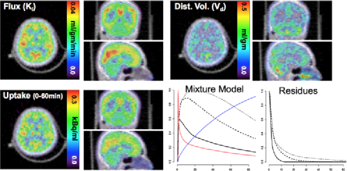
(b) Dynamic 7.5-minute PET-$H2O$ study in a normal subject

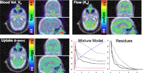
Figure 1: Color maps of selected kinetic parameters (cf. Section 2.1) recovered by residue analysis and the integrated uptake divided by study duration. Transverse, sagittal and coronal slices shown. The gray-scale images give tissue attenuation measured by the PET transmission scan. Line plots give the fitted mixture model [cf. $\bar{C}_{j}$ in equation (6)], including the arterial input ($C_{P}$ in red) and the Patlak component (blue). The normalized, non-Patlak, basis residues [$\bar{R}_{j}$ in equation (2.2)] are also shown on the right.

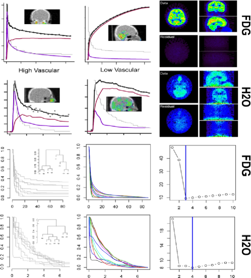
Figure 2: Top: Sample segment time-course data (points) and fitted step-function nonparametric residues (gray). The fitted residue-model time course (black line) is shown with vascular (purple) vs. nonvascular (brown) components: $C_{V}$ and $C_{E}$ after (3). Inserts show the intensity of the time course within the region of the segment. Right color maps show the distribution of the RMS for data and residuals from analysis (cf. Section 3.4). Bottom: (Left) Raw piecewise constant residues for segments (scaled to unity). A dendrogram obtained by clustering residues is also provided. (Center) Line plots are scaled B-spline-computed residues without retention [$\bar{R}_{j}$’s in (9)]. (Right) Risk values [$\hat{C}(J)$ in (10)] plotted against the number of components ($J$) in the mixture model—optimal number shown with blue line.

The H2O data come from a series reported in Muzi et al. (2009). The tracer dose (776 MBq) was injected over a 5-second time period. Dynamic PET imaging was carried out over a 7.9-minute time period ($T_{e}=7.9$). A set of $B=42$ time frames of data was acquired according to the following sampling: 1-minute pre-injection frame followed by 5 3-second frames, 10 6-second frames, 12 10-second frames, 8 15-second frames and ending with 6 20-second frames. Similar to FDG, a 10-region segmentation of the data was used to initialize the mixture model analysis, that is, $K=10$ in Section 3.2 (values of $K=20$ and $K=40$ were also considered but produced little or no change in results). The mixture model and associated normalized basis residues, apart from the constant residue component, had $4$ components; see Figure 1(b). Figure 1(b) shows total tracer uptake as well as computed values for vascular blood volume ($V_{B}$) and the distributional flow component ($K_{D}$). Note the vascular blood volume is elevated in the neighborhood of the internal carodits and the nasal cavity. The (distributional) flow pattern is elevated in the white and gray matter structures of the brain. In general, values of metabolic parameters are in agreement with those reported in the literature; cf. Muzi et al. (2009). Similar to FDG, the kinetic analysis here is seen to add to the information provided by uptake alone.

Figure 2 presents some diagnostic information for the analyses presented. Sample segments and the results of the associated nonparametric residue analysis are shown. The increased variability of H2O is evident. Even though the injected dose is larger than that of FDG, the shorter time frames and much shorter half-life of ¹⁵O results in lower radioactivity per time frame in the H2O study. Consequently, the data have more noise, as reflected in the displayed parameters. The voxel-level residual RMS characteristics of the fit are shown in Figure 2. For FDG, the RMS error is very small relative to the tracer uptake; in the case of H2O, the RMS error is generally higher relative to uptake, but there still does not appear to be a spatially coherent structure to the lack of fit. The fitted residue models for the selected segments are in good agreement with the data; see Figure 2. The decomposition of the time course of the fitted models show the vascular and nonvascular components of the fit [cf. equation (3)]. Note the time courses with high vascular contributions arise from well-known blood pools in the neck and nasal cavity; less vascular signals arise from white and grey matter tissue. The full set of fitted piecewise constant nonparametric residues [Hawe et al. (2012)] as well as the smoother residues produced by B-spline fitting [O’Sullivan et al. (2009)] are also shown in Figure 2. Note these latter residue curves only present the nonretained parts of the residues, that is, extraction is subtracted. The model selection criterion is plotted against the number of retained components. Three components are indicated for the FDG and four for the H2O data. A dendrogram for a hierarchical cluster analysis of the raw residues (normalized and adjusted for extraction) using a Euclidean distance matrix shows some exploratory support for the number of components selected. Note that, unlike the model selection statistic, the cluster analysis does not involve any recursive refitting of the time-course data. Overall, the analysis and diagnostics are very reasonable. A more detailed analysis over a series of similar cerebral studies is provided in the next section.

4.2 Cancer imaging examples

The use of PET for metabolic imaging of cancer and its response to therapy is of current clinical interest [Aboagye (2010), Krohn et al. (2007) and Mankoff et al. (2007)]. While PET-FDG imaging is an indicator of glucose metabolism, other aspects of cancer biology may also be useful. Cell proliferation, hypoxia, vascularity, drug resistance and cell death play important roles and the study of these processes in cancers with PET radiotracers is being explored with clinical imaging trails [Krohn et al. (2007)]. We present two examples to illustrate applications of our metabolic imaging procedure in such contexts. From a methodological viewpoint, these examples demonstrate the versatility of the residue imaging technique across a range of radiotracers and also in different target tissue volumes.

I. Brain tumor study

These data are from a series in Spence et al. (2009). The patient is a 39-year-old with recurrent right parietal anaplastic astrocytoma. The patient had follow-up clinical MR scans at 4 and 4.5 years after initial treatment with a combination of surgery, radiotherapy and chemotherapy. At the time of follow-up PET scans with ${}^{11}C$-labeled acetate (ACE), ${}^{11}C$-labeled carbon dioxide (CO2) and ¹⁸F-labeled fluoro-thymidine (FLT) were carried out. The ACE and CO2 studies were performed at the 4-year follow-up and the FLT at the 4.5-year follow-up. The focus of these PET scans was to study the potential for differentiation between tumor regional radionecrosis (residual but dead tissue) from tumor recurrence. This issue is difficult to decide on the basis of the standard clinical MR scan. Acetate flux is an indicator of membrane lipid synthesis [Yu et al. (2011)] and so may provide an early indicator of tumor recurrence. Metabolism of acetate produces carbon dioxide. As a result, the interpretation of acetate is somewhat confounded by processes associated with the fate of ${}^{11}C$ in carbon dioxide. The CO2 PET study is used to address this issue. FLT has the potential to provide information on the rate of thymidine utilization and this in turn is a potential indicator of cell proliferation.

Tracers were introduced by 1-minute intravenous infusion. The sampling protocols for ACE and CO2 were identical: Frame durations in seconds (some of which were repeated a number of times) were as follows: 5(18), 10(7), 20(4), 60(4), 180(4), 300(8) for a total of $B=45$ dynamic scans. With FLT there were $B=47$ frames: 10(10), 20(4), 40(3), 60(3), 120(5), 180(4), 300(18). An initial $K=10$ region segmentation was used for each data set. The selected mixture models have 5, 3 and 4 terms for ACE, CO2 and FLT. In each case, temporal and spatial diagnostics for the mixture model fit were satisfactory. Results of metabolic parameters are shown in Figure 3(a). The tumor region is apparent on both magnetic resonance (MR) scans. ACE flux is elevated in parts of this and these areas are also seen as high FLT flux. The CO2 flux is elevated in the brain ventricle/choroid plexus. The choroid plexus makes cerebral spinal fluid (CSF) in part by carbonic anhydrase to facilitate the exchange between CO2 and water and bicarbonate, and this starts in the cerebral ventricles. Thus, it makes physiologic sense that choroid plexus has high CO2 flux. There is an increased flow of FLT in the skull bone marrow and that is also elevated (perhaps as a result of blood-brain-barrier disruption) in the tumor. Note that the FLT flux is not substantially elevated in the marrow of the skull here. In normal circumstances this would be unexpected, however, because the marrow is lower on the side of the tumor, compared to the other side, this is likely a radiation effect. The increased FLT flux in the tumor region abnormality suggests enhanced cellular proliferation—possible tumor recurrence. The Spence et al. (2009) report found that FLT flux has potential as an imaging biomarker for distinguishing proliferation in patients with recurrent gliomas from radionecrosis, which has a similar MR pattern. There are a number of National Cancer Institute (NCI) sponsored trials underway that are investigating the potential of PET-FLT for guiding the treatment of cancer patients. The quantitation of flux and flow provided here enhances the understanding of the information provided by these studies.

(a) Brain tumor

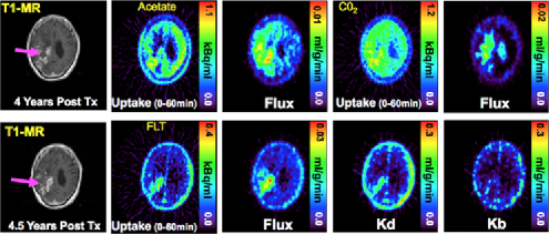
(b) Breast cancer

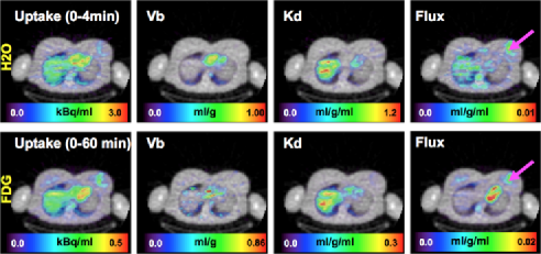
Figure 3: (a) Brain tumor 4 and 4.5 years after treatment. Standard clinical T1-weighted Magnetic Resonance images—tumor site indicated with pink arrow. Dynamic PET imaging with ${}^{11}C$ Acetate and ${}^{11}C$ $CO_{2}$ at 4-year follow-up were analyzed by residue analysis to obtain flux estimates. Dynamic ${}^{18}F$ fluoro-thymidine PET imaging was analyzed by residue analysis to obtain flux, $K_{d}$ and $K_{b}$ estimates. Transverse images through a representative plane of the tumor are shown. (b) Patient with locally advanced Breast Cancer imaged with PET-H2O and PET-FDG. Transverse slices of tracer uptake and residue calculated metabolic images of blood and distribution volume and flux. The grey scale is the measured tissue attenuation. The tumor site indicated with pink arrows.

II. Breast cancer

This data here is from a series of locally advanced breast cancer patients studied with PET FDG and H2O prior to treatment with neoadjuvant chemotherapy. The study, reported by Dunnwald et al. (2008), showed that the mismatch between H2O evaluated flow and FDG measured flux, provided a prognostic indicator of response and disease-free survival. A bolus intravenous injection of H2O was followed by dynamic PET image acquisition over a 7.75 minute period. A total of $B=53$ frames were obtained. A 1-minute pre-injection scan was followed by consecutive frames whose durations in seconds (with number of repeats) were as follows: 2(15), 5(14), 10(10), 15(8), 20(5). A short time later the FDG study was carried out. This entailed 2-minute intravenous infusion of FDG. A 1-minute pre-injection scan was followed by 24 further frames; these frame durations in seconds (including repeat number) were as follows: 20(4), 40(4), 60(4), 180(4), 300(4). There was no blood sampling, but analysis of the right ventricle of the heart region was used to extract an arterial input function in the analysis. Additional time courses for venous blood (vena-cava), the pulmonary veins and the right ventricle of the heart were also recovered from the PET image data; see Huang and O’Sullivan (2014) for details of the technique used. These signals were included as additional terms in the segmentation and mixture model analysis. In view of the increased range of tissue structures in the field of view, a greater number of segments ($K=15$) were used. Selected mixture models had 5 residue components for FDG and 4 for H2O. In each case temporal and spatial diagnostics for the mixture model fit were satisfactory. Parametric images are shown in Figure 3(b). The raw uptake patterns for the tracers do not differentiate between areas with high vascular uptake (heart cavity, liver) and areas with increased longer term retention (tumor and heart wall). The vascular and retention patterns are well described by images of blood volume ($V_{B}$), distributional flow ($K_{D}$) and flux ($K_{i}$). The increased apparent retention time of water in the tumor region (seen as a “flux” in the water residue analysis) may reflect that less effective vasculature often is associated with cancers, particular larger cancers; see Dunnwald et al. (2008) and Jain (2005). This is an example of a patient whose tumor has low blood flow and high FDG uptake, which is nicely captured by the analysis. The greatest FDG flux is in the section of the tumor at the edge of an apparent necrotic section, which makes sense as a place where blood flow would be low and FDG uptake might be high. We expect the flow measures to be similar from water and FDG [Tseng et al. (2004)], and the images support this.

5 Analysis of performance

We consider cerebral PET studies with FDG and H2O and examine aspects of the proposed methodology using both real and simulated data. One issue is to determine how regional averages of voxel-level residue estimates compare to regional residue estimates produced by analysis of regionally averaged time-course data. The latter issue is of interest because it is the common way that regional summaries of PET tracer kinetics are obtained. We used numerical simulations to explore this matter. A second issue is whether the approximation capabilities of our residue basis are adequate for real data. Recall the underlying mixture model is constructed adaptively by segmentation of the entire image volume. It is not clear if the derived mixture basis set has adequate local approximation characteristics. We compare our mixture modeling approach with an analysis of regionally averaged time-course data using standard compartment models.

5.1 Adaptive mixtures versus compartmental model residues

As previously indicated, the sample data sets used in Section 4.1 are taken from two series on normal subjects reported by Muzi et al. (2009) and Graham et al. (2002). In those series PET time-course data for a number of brain structures were recovered. With detailed reliance on co-registered high-resolution MR scans for anatomic reference, region of interest (ROI) PET time-course data for a number of brain structures were created. For FDG there were 10 regions in each of 12 studies to give a total of 120 ROI data sets. The regions were as follows: cerebellum, temporal, frontal, parietal and occipital cortex, thalamus, putamen, caudate, whole brain and white matter. For H2O, a set of 11 subjects was considered with each subject scanned twice. In each study between 6 and 9 regions were considered, giving a total of 184 ROI data sets. The regions included: choroid, pituitary and salivary gland, ventricle, selected whole brain regions, white and gray matter. In Muzi et al. (2009) and Graham et al. (2002), these ROI data were analyzed using the conventional compartmental models. Here we compare compartmental analysis of these H2O and FDG ROI data with analysis obtained using the adaptive mixture model recovered using the segmentation and recursive refinement algorithm of Section 3.1 and Section 3.2 of this paper. The mixture model was then applied to analyze the time-course data for each of the ROIs that had been recovered in the study, that is, application of the model in equation (11) to the ROI data. At the same time the ROI data were also analyzed using the relevant compartmental models. For reference, the ROI data were also analyzed using a fully nonparametric procedure with a piecewise constant residue [Hawe et al. (2012)]. In terms of fit, this gives an effective lower bound on what can be achieved for a given data set. Leave-out-one cross-validation residuals [Weisberg (1985)] were constructed for each analysis method, and the weighted sums of squares of these residuals were used for comparisons between different methods. Absolute cross-validated residuals from the mixture and compartmental approaches were also subjected to a paired Wilcoxon test [Wilcoxon (1945)]. The $p$-value for this test provides evidence against the hypothesis of similarity between the average magnitude of cross-validated residuals from the compartmental and mixture analysis. An overall comparison between the compartmental and mixture models is also carried out. A sign test is applied to the set of differences between the cross-validated residual sums of squares for the mixture and compartmental model. The mixture model is favored if the percentage of time it outperforms the compartmental model is significantly greater than 50%. We also compare compartmental and mixture model-based estimates of key kinetic parameters: flux ($K_{i}$) and distribution volume ($V_{D}$) for FDG and blood volume ($V_{B}$) and the distributional flow ($K_{D}$) for H2O. Note in the compartmental case this involves evaluating the fitted compartmental residue and then using the definitions in Section 2.1 to evaluate the resultant kinetic parameters.

(a) FDG data

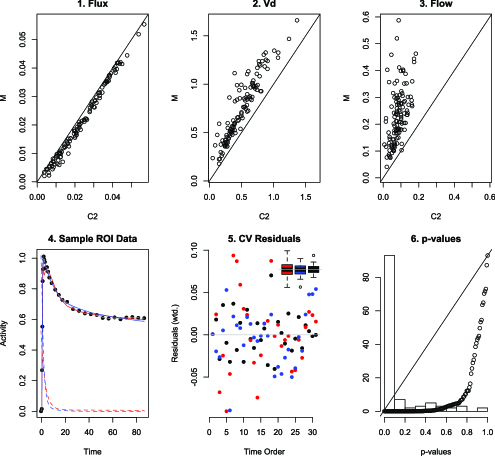
Figure 4: Comparison between selected kinetic parameters recovered from analysis of ROI data using compartmental (FDG and H2O) and mixture models $(1,2,3)$. 4. Sample ROI data (dots) together with fitted compartment, mixture and nonparametric analysis (red, blue and grey lines); fitted residues are shown with broken lines. 5. Color-coded leave-out-one cross-validated residuals. 6. Histogram and cumulative distribution (dots) of Wilcoxon $p$-values for paired comparison of the absolute CV-residuals of the compartmental and mixture models, line of identity included.

(b) H2O data

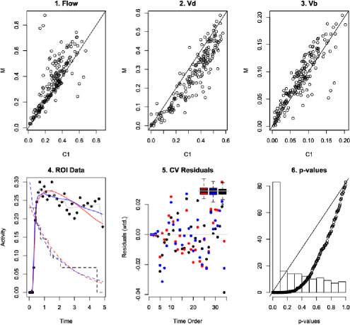
Figure 4: (Continued).

Results are presented in Figure 4. With FDG, the cross-validated residual sum of squares for the adaptive mixture models is lower than that for the 2-compartment model in 97 of the 120 ROIs examined (80% of cases). This is highly significant. In addition, the distribution of Wilcoxon $p$-values clearly favor the mixture model; see Figure 4(a)6. Results for H2O are not as strong. Here the adaptive mixture models is lower than that for the 1-compartmental model in 137 of the 184 ROIs examined (74% of cases). This is again highly significant. However, the distribution of Wilcoxon $p$-values [Figure 4(b)6], while still favoring the mixture model, is more uniform than was found for FDG. This reduced improvement in the mixture model is very likely a reflection of the higher noise which is evident in many of the H2O ROIs. Some representative sample time-course data and the models fit are also shown in Figures 4(a)4 and 4(b)4. In the high noise H2O example, the improvement in fit achieved by the mixture model is not so clear, however, there is little ambiguity in the FDG case. Figure 4 also reports comparisons between kinetic parameters recovered using the mixture and compartmental model analyses. Note the kinetics from the compartmental and mixture analysis are quite similar, particularly with flux and volume of distribution in FDG Figure 4(a)1–2. Discrepancies in flow values are apparent in Figure 4(a)3, with higher flow values being produced by the mixture analysis model. Somewhat noisier patterns are found with H2O. Flow and blood volume values obtained by the mixture analysis are on average higher than those of the compartmental model analysis; see Figure 4(b)1–3. The 1-compartmental model produces somewhat higher distribution volume values; see Figure 4(b)2. Given the model fit comparisons, parameters provided by mixture analysis are likely to be more reliable for FDG and H2O.

5.2 Simulation study

A prime motivation for mapping of residues at the voxel level is the simplicity with which the residue for a region can then be obtained, that is, by simply averaging the voxel-level residue estimates. If voxel-level data were measured without error, this approach would be guaranteed to yield the correct regional residue. However, one might have concern that with realistic noise, estimation at the voxel-level might be so poorly behaved that the regional averaging of voxel-level estimates would not produce good estimates of the target regional values. Here the residue recovered from analysis of the average time course for the region might be more accurate. We explore this issue in the context of the brain studies analyzed in Section 4.1. Recall those analyses involved consideration of $K=10$ segments, each with a characteristic time course: $y_{k}$ for $k=1,2,\ldots,K$. Each time course was subsequently represented as a linear combination of a reduced set of ($J$) basis residues as described in equations (4) and (2.2)—and modeled, similar to equation (11), as

$$y_{kb}=\mu_{kb}+w_{kb}^{-1/2}\varepsilon_{kb},$$

where $\mu_{kb}=\sum_{j=1}^{J}\alpha_{jk}\bar{\mu}_{jb}(\Delta_{k})$, $w_{kb}=1/{\mu_{kb}}$ and the errors $\varepsilon_{kb}$ are found to be approximately Guassian with mean zero and constant variance, say, $\phi_{k}^{2}$. Given that these data are from normal subjects, the configuration of the coefficients $\alpha_{\cdot k}=(\alpha_{1k},\alpha_{2k},\ldots,\alpha_{Jk})$ for the $K$ segments is realistic for normal cerebral PET studies with the FDG and H2O tracers. We bootstrap from these results to simulate voxel-level data for a set of $K$ synthetic regions of interest (ROIs).

The simulated data for the $i$th voxel in the $k$th region is generated by

$$y_{kib}=\tilde{\mu}_{kib}+\tilde{w}_{kib}^{-1/2}\tilde{\varepsilon}_{kib}$$ (16)

for $i=1,2,\ldots,N_{k}$ and $b=1,2,\ldots,B$. Here $\tilde{\mu}_{kib}=\sum_{j=1}^{J}\tilde{\alpha}_{ijk}\bar{\mu}_{jb}(\tilde{\Delta}_{ik})$ and $\tilde{w}_{kib}=1/{\tilde{\mu}_{kib}}$, with $\tilde{\varepsilon}_{kib}$, $\tilde{\Delta}_{ik}$ and $\tilde{\alpha}_{ijk}$ independent random variables. The measurement errors ($\tilde{\varepsilon}_{kib}$’s) are mean zero Gaussian with variance $N_{k}\phi_{k}^{2}$ for $i=1,2,\ldots,N_{k}$. Amplification of the variance by $N_{k}$ ensures the mean error over voxels has variance $\phi_{k}^{2}$; the delays ($\tilde{\Delta}_{ik}$’s) are log-normal with mean $\Delta_{k}$ and standard deviation proportional to the size of the region. The coefficient of variation is 20% in the largest region and, finally, the residue basis scales ($\tilde{\alpha}_{ijk}$’s) are generated from a Gamma distribution with mean $\alpha_{jk}$ and coefficient of variation set in proportion to the region size. The largest region has a coefficient of variation of 20%. This structure is designed to capture the intra-region voxel-to-voxel variation in terms of the time-of-arrival of the tracer, the voxel-to-voxel variation/heterogeneity in residues (including flow) and, of course, the quasi-Poisson measurement errors associated with PET instrumentation [Carson et al. (1993) and Huesman (1984)]. The overall scale of $\alpha$-coefficients is varied to achieve a range of six activity levels, equispaced on a logarithmic scale, the highest of which is 20 times larger than the lowest activity. The 10 regions had sizes ($N_{k}$) as follows: 20, 22, 39, 73, 85, 92, 93, 287, 345 and 1519 for FDG; 20, 31, 42, 128, 173, 195, 213, 394, 399 and 925 for H2O.

(a) FDG simulation

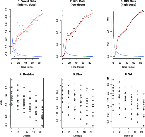
Figure 5: Sample time activity curve data (dots), together with the true (solid red) and fitted model (broken red) and the corresponding residues (blue)—1 (Voxel data), 2 and 3 (ROI data). Mean square error values (averaged over 50 replicates) for the residue 4 and two other parameters, 5 and 6 (flux and distribution volume for FDG and flow and distribution volume for H2O) plotted against dose ($\kappa$) for different regions. Regions are represented by separate symbols.

(b) H2O simulation

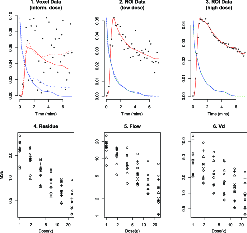
Figure 5: (Continued).

Sample voxel-level and mean ROI time-course data are shown in Figures 5(a)1–3 (FDG) and 5(b)1–3 (H2O). The intermediate activity/noise data are qualitatively similar to the data in Section 4.1. Sample residue estimates at the voxel and ROI levels are also shown in these same figures. Regional residues were computed in 2-ways, one based on analysis of the mean time-course data for the region and the other involving averaging of voxel-level residues. Voxel-level analysis could be done with and without imposition of positivity constraints on $\alpha$-coefficients. In high-noise environments, constrained estimators will be biased. The averaging of such estimators reinforces the voxel-level bias leading to a bias in the regional summary. In light of this, for quantitative regional analysis, the averaging of unconstrained voxel-level residues is recommended [Huang et al. (2013)].

Simulations involving data generation for 6 noise levels and 10 regions were repeated 50 times. Estimated residues were compared to true values directly using the integrated squared deviation and also in terms of squared deviation of key parameters, flux and distribution volume for FDG and flow and volume of distribution for H2O. The squared deviations were averaged over replicates to obtain estimates of mean square errors (MSE). The MSE for the averaged voxel-level estimators are plotted against dose in Figure 5(a)4–6 (FDG) and Figure 5(b)4–6 (H2O). A very similar pattern is found for the MSEs estimators produced by the analysis of the regionally averaged time-course data. A log-linear pattern is evident in Figure 5. MSEs vary by region, with larger regions having smaller MSEs. An analysis of the MSE data leads to

$$\log(\operatorname{MSE}_{lk})=\sum_{k}\beta_{k}\cdot I_{lk}-\gamma_{a}\cdot\log(\kappa_{lk})+\gamma_{M}\cdot M_{lk}+e_{lk},$$ (17)

where $\kappa_{lk}$ is dose level, $I_{lk}$ is the region indicator for region $k$ and $M_{lk}$ is an indicator of whether the estimator was evaluated by analysis of averaged time-course data or not. The modeling error is $e_{lk}$.

Table 1: MSE Characteristics for estimation of regional residues—parameters defined in the model in equation (17). $R^{2}$ values (adjusted) are from the model fit

Variable	$\bolds{\gamma_{a}}$	$\bolds{\gamma_{M}}$	$\bolds{R^{2}}$
FDG
Residue	0.96 ($\pm 0.02$)	$-0.03$ ($\pm 0.02$)	0.99
Flux	0.88 ($\pm 0.02$)	$-$0.05 ($\pm 0.02$)	0.99
$V_{D}$	0.98 ($\pm 0.02$)	$-0.01$ ($\pm 0.02$)	0.98
H2O
Residue	0.76 ($\pm 0.04$)	$-$0.01 ($\pm 0.04$)	0.84
Flow	0.66 ($\pm 0.07$)	$-$0.01 ($\pm 0.08$)	0.98
$V_{D}$	0.95 ($\pm 0.02$)	$-$0.01 ($\pm 0.02$)	0.99

Table 1 reports estimated values for the $\gamma_{a}$-coefficients. For FDG the $\hat{\gamma}_{a}\approx 1.0$, consistent with what one might expect in theory (see below). A slower rate ($\hat{\gamma}_{a}\approx 0.8$) is indicated for H2O, a reflection of the larger number of time frames (42 for H2O versus 31 for FDG) and the greater noise arising from the rapid decay of the ¹⁵O isotope. Larger regions generally have lower MSEs, but the heterogeneity of the region plays a role. As regards comparison between regional kinetic quantification by analysis of the averaged time course for the ROI or the averaging of voxel-level residues, there is little difference. With H2O there is some small (1%) degradation in MSE obtained by analysis of the average time-course data for the region; a similar result holds for Flux in FDG, although this is not the case for integrated squared error of the residue or the volume of distribution. This result supports mapping voxel-level residues because it allows subsequent analysis of regions of interest to be simply achieved by direct application of ROIs to voxel-level residue information.

Theoretical interpretation of results

At high doses MSE can be expected to be dominated by variance. Since equation (16) is a linear model, the covariance of the estimated $\alpha$-coefficients at the $i$th voxel, which are obtained by a weighted least squares procedure, will be approximated by $\Sigma_{\alpha}\approx\phi^{2}[X^{\prime}WX]^{-1}$, where

$$X^{\prime}WX_{jj^{\prime}}=\sum_{b}w_{b}\bar{\mu}_{jb}(\hat{\Delta})\bar{\mu}_{j^{\prime}b}(\hat{\Delta})$$

and $w_{b}=\sum_{j}\hat{\alpha}_{j}\bar{\mu}_{jb}(\hat{\Delta})$. Here, to simplify the notation, we have dropped the subscripts $i$ and $k$. This variance approximation will become more reliable at high doses when the constraints on the $\alpha$-coefficients are, typically, not active. Recall from equation (7), $\bar{\mu}_{jb}$ involves the convolution of the normalized residue $\bar{R}_{j}$ and the arterial input function, $C_{p}$. So if $C_{p}$ is expressed as $C_{p}=\kappa\bar{C}_{p}$ where $\bar{C}_{p}$ has amplitude of unity, $\Sigma_{\alpha}$ can be expressed as

$$\Sigma_{\alpha}=\kappa^{-1}\phi^{2}\bigl{[}\bar{X}^{\prime}\bar{W}\bar{X}\bigr{]}^{-1},$$ (18)

with $\bar{X}^{\prime}\bar{W}\bar{X}$ the same as $X^{\prime}WX$ but with $\bar{\mu}_{jb}$ now involving convolution of the normalized residue and normalized arterial input $\bar{C}_{p}$. Thus, at high doses the variance and, consequently, the MSE, will be inversely proportional to dose ($\kappa$). This is consistent with $\hat{\gamma}_{a}\approx 1$, as was found for FDG in the simulation. The slower convergence ($\hat{\gamma}_{a}\approx 0.8$) for H2O may be a reflection of a greater dependence on constraints, due to the higher noise. When constraints are active, the standard weighted least squares covariance formula will not be reliable.

6 Discussion

We have presented an approach to the estimation of voxel-level tracer residues from PET time-course data. The technique uses a data-adaptive mixture model that allows for voxel-level variation in the time of arrival of the tracer in the arterial supply. The mixture representation of local residues is plausible and has been used previously with basis residues that are a compartmental model or have simple exponential forms [Cunningham and Jones (1993) and O’Sullivan (1993)]. The present work shows that it is possible to also use nonparametric forms for the basis residues. This allows the possibility to better investigate potential deviations from compartmental-like descriptions of tissue residues. Computationally, the linearity of mixture models is attractive, as it facilitates the implementation based on efficient use of standard quadratic programming tools. The work has a reliance on multivariate statistical methods and uses backward elimination guided by an unbiased risk type model selection statistic.

Residue functions are life tables for the transit time of radiotracer atoms. Just as infant and elderly mortality patterns might be given separate attention in a human life table, decomposition of the residue can provide insight into the tracer kinetics. Our approach emphasizes decomposition of residue to focus on flow and volume characteristics of vascular and in distribution transport as well as the (apparent) rate of extraction of the tracer by tissue, that is, flux. Thus, we have a 5-number summary for the residue. The life-table perspective on the tissue residue emphasized in this paper may encourage broader interest in adapting methods from mainstream survival analysis for application to the growing needs for quantitation in PET studies and for related contrast tracking techniques used in computerized tomography and magnetic resonance [Schmid et al. (2009)].

PET imaging has grown in importance particularly in the context of cancer, where over 90% of clinical imaging with PET is carried out. Having more sophisticated kinetic analysis tools, such as residue analysis, can enhance the type of information recovered from these studies. This may potentially lead to better procedures for selecting and monitoring cancer treatments in order to optimize the patient outcomes. A number of current clinical imaging trails with PET in cancer already have reliance on detailed kinetic analysis for extraction of diagnostic information. Given the nature of the problems involved, there is an opportunity for statistics to play a greater role in these developments.

References

- Aboagye (2010) {barticle}[auto:STB—2014/02/12—14:17:21] \bauthor\bsnmAboagye, \bfnmE. O.\binitsE. O. (\byear2010). \btitleThe future of imaging: Developing the tools for monitoring response to therapy in oncology: The 2009 Sir James MacKenzie Davidson memorial lecture. \bjournalBr. J. Radiol. \bvolume83 \bpages814–822. \bptokimsref\endbibitem
- Akaike (1974) {barticle}[mr] \bauthor\bsnmAkaike, \bfnmHirotugu\binitsH. (\byear1974). \btitleA new look at the statistical model identification. \bjournalIEEE Trans. Automat. Control \bvolumeAC-19 \bpages716–723. \bidissn=0018-9286, mr=0423716 \bptokimsref\endbibitem
- Bassingthwaighte (1970) {barticle}[pbm] \bauthor\bsnmBassingthwaighte, \bfnmJ. B.\binitsJ. B. (\byear1970). \btitleBlood flow and diffusion through mammalian organs. \bjournalScience \bvolume167 \bpages1347–1353. \bidissn=0036-8075, mid=NIHMS233670, pmcid=3004783, pmid=4904998 \bptokimsref\endbibitem
- Bassingthwaighte (2000) {barticle}[pbm] \bauthor\bsnmBassingthwaighte, \bfnmJ. B.\binitsJ. B. (\byear2000). \btitleStrategies for the physiome project. \bjournalAnn. Biomed. Eng. \bvolume28 \bpages1043–1058. \bidissn=0090-6964, mid=NIHMS197460, pmcid=3425440, pmid=11144666 \bptokimsref\endbibitem
- Carson et al. (1993) {barticle}[auto:STB—2014/02/12—14:17:21] \bauthor\bsnmCarson, \bfnmR. E.\binitsR. E., \bauthor\bsnmYan, \bfnmY.\binitsY., \bauthor\bsnmDaube-Witherspoon, \bfnmM. E.\binitsM. E., \bauthor\bsnmFreedman, \bfnmN.\binitsN., \bauthor\bsnmBacharach, \bfnmS. L.\binitsS. L. and \bauthor\bsnmHerscovitch, \bfnmP.\binitsP. (\byear1993). \btitleAn approximation formula for PET region-of-interest values. \bjournalIEEE Trans. Med. Imag. \bvolume12 \bpages240–251. \bptokimsref\endbibitem
- Cox and Oakes (2001) {bbook}[mr] \bauthor\bsnmCox, \bfnmD. R.\binitsD. R. and \bauthor\bsnmOakes, \bfnmD.\binitsD. (\byear2001). \btitleAnalysis of Survival Data. \bpublisherChapman & Hall, \blocationLondon. \bptnotecheck year \bptokimsref\endbibitem
- Cunningham and Jones (1993) {barticle}[auto:STB—2014/02/12—14:17:21] \bauthor\bsnmCunningham, \bfnmV. J.\binitsV. J. and \bauthor\bsnmJones, \bfnmT.\binitsT. (\byear1993). \btitleSpectral analysis of dynamic PET studies. \bjournalJ. Cereb. Blood Flow Metab. \bvolume13 \bpages15–23. \bptokimsref\endbibitem
- Dunnwald et al. (2008) {barticle}[auto:STB—2014/02/12—14:17:21] \bauthor\bsnmDunnwald, \bfnmL. K.\binitsL. K., \bauthor\bsnmGralow, \bfnmJ. R.\binitsJ. R., \bauthor\bsnmEllis, \bfnmG. K.\binitsG. K., \bauthor\bsnmLivingston, \bfnmR. B.\binitsR. B., \bauthor\bsnmLinden, \bfnmH. M.\binitsH. M., \bauthor\bsnmSpecht, \bfnmJ. M.\binitsJ. M., \bauthor\bsnmDoot, \bfnmR. K.\binitsR. K., \bauthor\bsnmLawton, \bfnmT. J.\binitsT. J., \bauthor\bsnmBarlow, \bfnmW. E.\binitsW. E., \bauthor\bsnmKurland, \bfnmB. F.\binitsB. F., \bauthor\bsnmSchubert, \bfnmE. K.\binitsE. K. and \bauthor\bsnmMankoff, \bfnmD. A.\binitsD. A. (\byear2008). \btitleTumor metabolism and blood flow changes by positron emission tomography: Relation to survival in patients treated with neo-adjuvant chemotherapy for locally advanced breast cancer. \bjournalJ. Clin. Oncol. \bvolume20 \bpages4449–4457. \bptokimsref\endbibitem
- Graham et al. (2002) {barticle}[auto:STB—2014/02/12—14:17:21] \bauthor\bsnmGraham, \bfnmM. M.\binitsM. M., \bauthor\bsnmMuzi, \bfnmM.\binitsM., \bauthor\bsnmSpence, \bfnmA. M.\binitsA. M., \bauthor\bsnmO’Sullivan, \bfnmF.\binitsF., \bauthor\bsnmLewellen, \bfnmT. K.\binitsT. K., \bauthor\bsnmLimk, \bfnmJ. M.\binitsJ. M. and \bauthor\bsnmKrohn, \bfnmK. A.\binitsK. A. (\byear2002). \btitleThe fluorodeoxyglucose lumped constant in normal human brain. \bjournalJ. Nucl. Med. \bvolume43 \bpages1157–1166. \bptokimsref\endbibitem
- Gunn et al. (2002) {barticle}[auto:STB—2014/02/12—14:17:21] \bauthor\bsnmGunn, \bfnmR. N.\binitsR. N., \bauthor\bsnmGunn, \bfnmS. R.\binitsS. R., \bauthor\bsnmTurkheimer, \bfnmF. E.\binitsF. E., \bauthor\bsnmAston, \bfnmJ. A. D.\binitsJ. A. D. and \bauthor\bsnmCunningham, \bfnmV. J.\binitsV. J. (\byear2002). \btitlePositron emission tomography compartmental models: A basis pursuit strategy for kinetic modeling. \bjournalJ. Cereb. Blood Flow Metab. \bvolume22 \bpages1425–1439. \bptokimsref\endbibitem
- Hawe et al. (2012) {barticle}[auto:STB—2014/02/12—14:17:21] \bauthor\bsnmHawe, \bfnmD.\binitsD., \bauthor\bsnmHernández Fernández, \bfnmF.\binitsF., \bauthor\bsnmO’Suilleabháin, \bfnmL.\binitsL., \bauthor\bsnmHuang, \bfnmJ.\binitsJ., \bauthor\bsnmWolsztynski, \bfnmE.\binitsE. and \bauthor\bsnmO’Sullivan, \bfnmF.\binitsF. (\byear2012). \btitleKinetic analysis of dynamic positron emission tomography data using open-source image processing and statistical inference tools. \bjournalWIREs Comput. Stat. \bvolume4 \bpages316–322. \biddoi=10.1002/wics.1196 \bptokimsref\endbibitem
- Huang and O’Sullivan (2014) {bmisc}[auto:STB—2014/02/12—14:17:21] \bauthor\bsnmHuang, \bfnmJ.\binitsJ. and \bauthor\bsnmO’Sullivan, \bfnmF.\binitsF. (\byear2014). \bhowpublishedAn analysis of whole body tracer kinetics in dynamic PET studies with application to image-based blood input function extraction. In IEEE Transactions on Medical Imaging. DOI:\doiurl10.1109/TMI.2014.2305113. \bptokimsref\endbibitem
- Huang and Phelps (1986) {bmisc}[auto:STB—2014/02/12—14:17:21] \bauthor\bsnmHuang, \bfnmS. C.\binitsS. C. and \bauthor\bsnmPhelps, \bfnmM. E.\binitsM. E. (\byear1986). \bhowpublishedPrinciples of tracer kinetic modeling in positron emission tomography and autoradiography. In Positron Emission Tomography and Autoradiography (M. E. Phelps, J. C. Mazziotta and H. R. Schelbert, eds.) 287–346. Raven, New York. \bptokimsref\endbibitem
- Huang et al. (2013) {bmisc}[auto:STB—2014/02/12—14:17:21] \bauthor\bsnmHuang, \bfnmJ.\binitsJ., \bauthor\bsnmWolsztynski, \bfnmE.\binitsE., \bauthor\bsnmMuzi, \bfnmM.\binitsM., \bauthor\bsnmRoychoudhury, \bfnmK.\binitsK., \bauthor\bsnmKim, \bfnmK.\binitsK. and \bauthor\bsnmO’Sullivan, \bfnmF.\binitsF. (\byear2013). \bhowpublishedA cautionary note on the use of constrained reconstructions for quantification of regional PET imaging data. In IEEE Conference Record NSS-MIC. Seoul, South Korea. \bptokimsref\endbibitem
- Huesman (1984) {barticle}[auto:STB—2014/02/12—14:17:21] \bauthor\bsnmHuesman, \bfnmR. H.\binitsR. H. (\byear1984). \btitleA new fast algorithm for the evaluation of regions of interest and statistical uncertainty in computed tomography. \bjournalPhys. Med. Biol. \bvolume29 \bpages543–552. \bptokimsref\endbibitem
- Jain (2005) {barticle}[auto:STB—2014/02/12—14:17:21] \bauthor\bsnmJain, \bfnmR. K.\binitsR. K. (\byear2005). \btitleNormalization of tumor vasculature: An emerging concept in antiangiogenic therapy. \bjournalScience \bvolume307 \bpages58–62. \bptokimsref\endbibitem
- Kaasinen et al. (2005) {barticle}[auto:STB—2014/02/12—14:17:21] \bauthor\bsnmKaasinen, \bfnmV.\binitsV., \bauthor\bsnmMaguire, \bfnmR. P.\binitsR. P., \bauthor\bsnmHundemer, \bfnmH. P.\binitsH. P. and \bauthor\bsnmLeenders, \bfnmK. L.\binitsK. L. (\byear2005). \btitleCorticostriatal covariance patterns of 6-[(18)F]fluoro-L-dopa and [(18)F]fluorodeoxyglucose PET in Parkinson’s disease. \bjournalJ. Neurol. \bvolume253 \bpages340–348. \bptokimsref\endbibitem
- Krohn et al. (2007) {barticle}[pbm] \bauthor\bsnmKrohn, \bfnmKenneth A.\binitsK. A., \bauthor\bsnmO’Sullivan, \bfnmFinbarr\binitsF., \bauthor\bsnmCrowley, \bfnmJohn\binitsJ., \bauthor\bsnmEary, \bfnmJanet F.\binitsJ. F., \bauthor\bsnmLinden, \bfnmHannah M.\binitsH. M., \bauthor\bsnmLink, \bfnmJeanne M.\binitsJ. M., \bauthor\bsnmMankoff, \bfnmDavid A.\binitsD. A., \bauthor\bsnmMuzi, \bfnmMark\binitsM., \bauthor\bsnmRajendran, \bfnmJoseph G.\binitsJ. G., \bauthor\bsnmSpence, \bfnmAlexander M.\binitsA. M. and \bauthor\bsnmSwanson, \bfnmKristin R.\binitsK. R. (\byear2007). \btitleChallenges in clinical studies with multiple imaging probes. \bjournalNucl. Med. Biol. \bvolume34 \bpages879–885. \biddoi=10.1016/j.nucmedbio.2007.07.014, issn=0969-8051, mid=NIHMS32840, pii=S0969-8051(07)00194-1, pmcid=2099630, pmid=17921038 \bptokimsref\endbibitem
- Lawless (2003) {bbook}[mr] \bauthor\bsnmLawless, \bfnmJerald F.\binitsJ. F. (\byear2003). \btitleStatistical Models and Methods for Lifetime Data, \bedition2nd ed. \bpublisherWiley, \blocationHoboken, NJ. \bidmr=1940115 \bptokimsref\endbibitem
- Layfield and Venegas (2005) {barticle}[pbm] \bauthor\bsnmLayfield, \bfnmDominick\binitsD. and \bauthor\bsnmVenegas, \bfnmJosé G.\binitsJ. G. (\byear2005). \btitleEnhanced parameter estimation from noisy PET data: Part I—Methodology. \bjournalAcad. Radiol. \bvolume12 \bpages1440–1447. \biddoi=10.1016/j.acra.2005.08.012, issn=1076-6332, pii=S1076-6332(05)00672-0, pmid=16253856 \bptokimsref\endbibitem
- Lee et al. (2005) {barticle}[auto:STB—2014/02/12—14:17:21] \bauthor\bsnmLee, \bfnmJ. S.\binitsJ. S., \bauthor\bsnmLee, \bfnmD. S.\binitsD. S., \bauthor\bsnmAhn, \bfnmJ. Y.\binitsJ. Y., \bauthor\bsnmCheon, \bfnmG. J.\binitsG. J., \bauthor\bsnmKim, \bfnmS. K.\binitsS. K., \bauthor\bsnmYeo, \bfnmJ. S.\binitsJ. S., \bauthor\bsnmPark, \bfnmK. S.\binitsK. S., \bauthor\bsnmChung, \bfnmJ. K.\binitsJ. K. and \bauthor\bsnmLee, \bfnmM. C.\binitsM. C. (\byear2005). \btitleParametric image of myocardial blood flow generated from dynamic H2(15)O PET using factor analysis and cluster analysis. \bjournalMed. Biol. Eng. Comput. \bvolume43 \bpages678–685. \bptokimsref\endbibitem
- Li, Yipintsoi and Bassingthwaighte (1997) {barticle}[auto:STB—2014/02/12—14:17:21] \bauthor\bsnmLi, \bfnmZ.\binitsZ., \bauthor\bsnmYipintsoi, \bfnmT.\binitsT. and \bauthor\bsnmBassingthwaighte, \bfnmJ. B.\binitsJ. B. (\byear1997). \btitleModeling blood flow heterogeneity. \bjournalAnnals of Biomedical Engineering \bvolume25 \bpages604–619. \bptokimsref\endbibitem
- Maitra and O’Sullivan (1998) {barticle}[mr] \bauthor\bsnmMaitra, \bfnmRanjan\binitsR. and \bauthor\bsnmO’Sullivan, \bfnmFinbarr\binitsF. (\byear1998). \btitleVariability assessment in positron emission tomography and related generalized deconvolution models. \bjournalJ. Amer. Statist. Assoc. \bvolume93 \bpages1340–1355. \biddoi=10.2307/2670050, issn=0162-1459, mr=1666632 \bptokimsref\endbibitem
- Mankoff et al. (2007) {barticle}[pbm] \bauthor\bsnmMankoff, \bfnmDavid A.\binitsD. A., \bauthor\bsnmO’Sullivan, \bfnmFinbarr\binitsF., \bauthor\bsnmBarlow, \bfnmWilliam E.\binitsW. E. and \bauthor\bsnmKrohn, \bfnmKenneth A.\binitsK. A. (\byear2007). \btitleMolecular imaging research in the outcomes era: Measuring outcomes for individualized cancer therapy. \bjournalAcad. Radiol. \bvolume14 \bpages398–405. \biddoi=10.1016/j.acra.2007.01.005, issn=1076-6332, mid=NIHMS21077, pii=S1076-6332(07)00009-8, pmcid=1868571, pmid=17368207 \bptokimsref\endbibitem
- McCullagh and Nelder (1983) {bbook}[mr] \bauthor\bsnmMcCullagh, \bfnmP.\binitsP. and \bauthor\bsnmNelder, \bfnmJ. A.\binitsJ. A. (\byear1983). \btitleGeneralized Linear Models. \bpublisherChapman & Hall, \blocationLondon. \bidmr=0727836 \bptokimsref\endbibitem
- Meier and Zierler (1954) {barticle}[pbm] \bauthor\bsnmMeier, \bfnmP.\binitsP. and \bauthor\bsnmZierler, \bfnmK. L.\binitsK. L. (\byear1954). \btitleOn the theory of the indicator-dilution method for measurement of blood flow and volume. \bjournalJ. Appl. Physiol. \bvolume6 \bpages731–744. \bidissn=0021-8987, pmid=13174454 \bptokimsref\endbibitem
- Murase (2003) {barticle}[pbm] \bauthor\bsnmMurase, \bfnmKenya\binitsK. (\byear2003). \btitleSpectral analysis: Principle and clinical applications. \bjournalAnn. Nucl. Med. \bvolume17 \bpages427–434. \bidissn=0914-7187, pmid=14575374 \bptokimsref\endbibitem
- Muzi et al. (2009) {barticle}[pbm] \bauthor\bsnmMuzi, \bfnmMark\binitsM., \bauthor\bsnmMankoff, \bfnmDavid A.\binitsD. A., \bauthor\bsnmLink, \bfnmJeanne M.\binitsJ. M., \bauthor\bsnmShoner, \bfnmSteve\binitsS., \bauthor\bsnmCollier, \bfnmAnn C.\binitsA. C., \bauthor\bsnmSasongko, \bfnmLucy\binitsL. and \bauthor\bsnmUnadkat, \bfnmJashvant D.\binitsJ. D. (\byear2009). \btitleImaging of cyclosporine inhibition of P-glycoprotein activity using 11C-verapamil in the brain: Studies of healthy humans. \bjournalJ. Nucl. Med. \bvolume50 \bpages1267–1275. \biddoi=10.2967/jnumed.108.059162, issn=0161-5505, mid=NIHMS145104, pii=jnumed.108.059162, pmcid=2754733, pmid=19617341 \bptokimsref\endbibitem
- Muzi et al. (2012) {barticle}[auto:STB—2014/02/12—14:17:21] \bauthor\bsnmMuzi, \bfnmM.\binitsM., \bauthor\bsnmO’Sullivan, \bfnmF.\binitsF., \bauthor\bsnmMankoff, \bfnmD. A.\binitsD. A., \bauthor\bsnmDoot, \bfnmR. K.\binitsR. K., \bauthor\bsnmPierce, \bfnmL. A.\binitsL. A., \bauthor\bsnmKurland, \bfnmB. F.\binitsB. F., \bauthor\bsnmLinden, \bfnmH. M.\binitsH. M. and \bauthor\bsnmKinahan, \bfnmP. E.\binitsP. E. (\byear2012). \btitleQuantitative assessment of dynamic PET imaging data in cancer imaging. \bjournalMagn. Reson. Imaging. \bvolume30 \bpages1203–1215. \bptokimsref\endbibitem
- Natterer and Wübbeling (2001) {bbook}[mr] \bauthor\bsnmNatterer, \bfnmF.\binitsF. and \bauthor\bsnmWübbeling, \bfnmF.\binitsF. (\byear2001). \btitleMathematical Methods in Image Reconstruction. \bpublisherSIAM, \blocationPhiladelphia, PA. \bidmr=1828933 \bptokimsref\endbibitem
- O’Sullivan (1993) {barticle}[pbm] \bauthor\bsnmO’Sullivan, \bfnmF.\binitsF. (\byear1993). \btitleImaging radiotracer model parameters in PET: A mixture analysis approach. \bjournalIEEE Trans. Med. Imaging \bvolume12 \bpages399–412. \biddoi=10.1109/42.241867, issn=0278-0062, pmid=18218432 \bptokimsref\endbibitem
- O’Sullivan (2006) {barticle}[auto:STB—2014/02/12—14:17:21] \bauthor\bsnmO’Sullivan, \bfnmF.\binitsF. (\byear2006). \btitleLocally constrained mixture representation of dynamic imaging data from PET and MR studies. \bjournalBiostatistics \bvolume7 \bpages318–338. \bptokimsref\endbibitem
- O’Sullivan and Pawitan (1996) {barticle}[auto] \bauthor\bsnmO’Sullivan, \bfnmF.\binitsF. and \bauthor\bsnmYudi, \bfnmP.\binitsP. (\byear1996). \btitleBandwidth selection for indirect density estimation based on corrupted histogram data. \bjournalJ. Amer. Statist. Assoc. \bvolume91 \bpages610–626. \bidmr=1395729 \bptokimsref\endbibitem
- O’Sullivan et al. (2009) {barticle}[mr] \bauthor\bsnmO’Sullivan, \bfnmFinbarr\binitsF., \bauthor\bsnmMuzi, \bfnmMark\binitsM., \bauthor\bsnmSpence, \bfnmAlexander M.\binitsA. M., \bauthor\bsnmMankoff, \bfnmDavid M.\binitsD. M., \bauthor\bsnmO’Sullivan, \bfnmJanet N.\binitsJ. N., \bauthor\bsnmFitzgerald, \bfnmNiall\binitsN., \bauthor\bsnmNewman, \bfnmGeorge C.\binitsG. C. and \bauthor\bsnmKrohn, \bfnmKenneth A.\binitsK. A. (\byear2009). \btitleNonparametric residue analysis of dynamic PET data with application to cerebral FDG studies in normals. \bjournalJ. Amer. Statist. Assoc. \bvolume104 \bpages556–571. \biddoi=10.1198/jasa.2009.0021, issn=0162-1459, mr=2751438 \bptokimsref\endbibitem
- Ostergaard et al. (1999) {barticle}[auto:STB—2014/02/12—14:17:21] \bauthor\bsnmOstergaard, \bfnmL.\binitsL., \bauthor\bsnmChesler, \bfnmD. A.\binitsD. A., \bauthor\bsnmWeisskoff, \bfnmR. M.\binitsR. M., \bauthor\bsnmSorensen, \bfnmA. G.\binitsA. G. and \bauthor\bsnmRosen, \bfnmB. R.\binitsB. R. (\byear1999). \btitleModeling cerebral blood flow and flow heterogeneity from magnetic resonance residue data. \bjournalMagn. Reson. Med. \bvolume19 \bpages690–699. \bptokimsref\endbibitem
- Patlak, Blasberg and Fenstermacher (1983) {barticle}[auto:STB—2014/02/12—14:17:21] \bauthor\bsnmPatlak, \bfnmC. S.\binitsC. S., \bauthor\bsnmBlasberg, \bfnmR. G.\binitsR. G. and \bauthor\bsnmFenstermacher, \bfnmJ. D.\binitsJ. D. (\byear1983). \btitleGraphical evaluation of blood-to-brain transfer constants from multiple-time uptake data. \bjournalJ. Cereb. Blood Flow Metab. \bvolume3 \bpages1–7. \bptokimsref\endbibitem
- Phelps (2000) {barticle}[auto:STB—2014/02/12—14:17:21] \bauthor\bsnmPhelps, \bfnmM. E.\binitsM. E. (\byear2000). \btitlePositron emission tomography provides molecular imaging of biological processes. \bjournalProc. Natl. Acad. Sci. USA \bvolume97 \bpages9226–9233. \bptokimsref\endbibitem
- Phelps et al. (1979) {barticle}[auto:STB—2014/02/12—14:17:21] \bauthor\bsnmPhelps, \bfnmM. E.\binitsM. E., \bauthor\bsnmHuang, \bfnmS. C.\binitsS. C., \bauthor\bsnmHoffman, \bfnmE. J.\binitsE. J., \bauthor\bsnmSelin, \bfnmC.\binitsC., \bauthor\bsnmSokoloff, \bfnmL.\binitsL. and \bauthor\bsnmKuhl, \bfnmD. E.\binitsD. E. (\byear1979). \btitleTomographic measurement of local cerebral glucose metabolic rate in humans with [F-18]2-Fluoro-2-deoxy-D-glucose: Validation of method. \bjournalAnn. Neurol. \bvolume6 \bpages371–388. \bptokimsref\endbibitem
- Provenzale et al. (2008) {barticle}[auto:STB—2014/02/12—14:17:21] \bauthor\bsnmProvenzale, \bfnmJ. M.\binitsJ. M., \bauthor\bsnmShah, \bfnmK.\binitsK., \bauthor\bsnmPatel, \bfnmU.\binitsU. and \bauthor\bsnmMcCrory, \bfnmD. C.\binitsD. C. (\byear2008). \btitleSystematic review of CT and MR perfusion imaging for assessment of acute cerebrovascular disease. \bjournalAm. J. Neuroradiol. \bvolume29 \bpages1476–1482. \bptokimsref\endbibitem
- Schmid et al. (2009) {barticle}[auto:STB—2014/02/12—14:17:21] \bauthor\bsnmSchmid, \bfnmV. J.\binitsV. J., \bauthor\bsnmWhitcher, \bfnmB.\binitsB., \bauthor\bsnmPadhani, \bfnmA. R.\binitsA. R. and \bauthor\bsnmYang, \bfnmG.-Z.\binitsG.-Z. (\byear2009). \btitleA semi-parametric technique for the quantitative analysis of dynamic contrast-enhanced MR images based on Bayesian P-splines. \bjournalIEEE Transactions in Medical Imaging \bvolume28 \bpages789–798. \bptokimsref\endbibitem
- Spence et al. (2009) {barticle}[pbm] \bauthor\bsnmSpence, \bfnmAlexander M.\binitsA. M., \bauthor\bsnmMuzi, \bfnmMark\binitsM., \bauthor\bsnmLink, \bfnmJeanne M.\binitsJ. M., \bauthor\bsnmO’Sullivan, \bfnmFinbarr\binitsF., \bauthor\bsnmEary, \bfnmJanet F.\binitsJ. F., \bauthor\bsnmHoffman, \bfnmJohn M.\binitsJ. M., \bauthor\bsnmShankar, \bfnmLalitha K.\binitsL. K. and \bauthor\bsnmKrohn, \bfnmKenneth A.\binitsK. A. (\byear2009). \btitleNCI-sponsored trial for the evaluation of safety and preliminary efficacy of 3’-deoxy-3’-[18F]fluorothymidine (FLT) as a marker of proliferation in patients with recurrent gliomas: Preliminary efficacy studies. \bjournalMol. Imaging Biol. \bvolume11 \bpages343–355. \biddoi=10.1007/s11307-009-0215-2, issn=1860-2002, pmid=19326172 \bptokimsref\endbibitem
- Tseng et al. (2004) {barticle}[pbm] \bauthor\bsnmTseng, \bfnmJeffrey\binitsJ., \bauthor\bsnmDunnwald, \bfnmLisa K.\binitsL. K., \bauthor\bsnmSchubert, \bfnmErin K.\binitsE. K., \bauthor\bsnmLink, \bfnmJeanne M.\binitsJ. M., \bauthor\bsnmMinoshima, \bfnmSatoshi\binitsS., \bauthor\bsnmMuzi, \bfnmMark\binitsM. and \bauthor\bsnmMankoff, \bfnmDavid A.\binitsD. A. (\byear2004). \btitle18F-FDG kinetics in locally advanced breast cancer: Correlation with tumor blood flow and changes in response to neoadjuvant chemotherapy. \bjournalJ. Nucl. Med. \bvolume45 \bpages1829–1837. \bidissn=0161-5505, pii=45/11/1829, pmid=15534051 \bptokimsref\endbibitem
- Veronese et al. (2013) {barticle}[pbm] \bauthor\bsnmVeronese, \bfnmMattia\binitsM., \bauthor\bsnmRizzo, \bfnmGaia\binitsG., \bauthor\bsnmTurkheimer, \bfnmFederico E.\binitsF. E. and \bauthor\bsnmBertoldo, \bfnmAlessandra\binitsA. (\byear2013). \btitleSAKE: A new quantification tool for positron emission tomography studies. \bjournalComput. Methods Programs Biomed. \bvolume111 \bpages199–213. \biddoi=10.1016/j.cmpb.2013.03.016, issn=1872-7565, pii=S0169-2607(13)00106-5, pmid=23611334 \bptokimsref\endbibitem
- Weisberg (1985) {bbook}[mr] \bauthor\bsnmWeisberg, \bfnmSanford\binitsS. (\byear1985). \btitleApplied Linear Regression. \bpublisherWiley, \blocationHoboken, NJ. \bptokimsref\endbibitem
- Wilcoxon (1945) {barticle}[auto:STB—2014/02/12—14:17:21] \bauthor\bsnmWilcoxon, \bfnmF.\binitsF. (\byear1945). \btitleIndividual comparisons by ranking methods. \bjournalBiometrics Bulletin \bvolume1 \bpages80–83. \bptokimsref\endbibitem
- Yu et al. (2011) {barticle}[auto:STB—2014/02/12—14:17:21] \bauthor\bsnmYu, \bfnmE. Y.\binitsE. Y., \bauthor\bsnmMuzi, \bfnmM.\binitsM., \bauthor\bsnmHackenbracht, \bfnmJ. A.\binitsJ. A., \bauthor\bsnmRezvani, \bfnmB. B.\binitsB. B., \bauthor\bsnmLink, \bfnmJ. M.\binitsJ. M., \bauthor\bsnmMontgomery, \bfnmR. B.\binitsR. B., \bauthor\bsnmHigano, \bfnmC. S.\binitsC. S., \bauthor\bsnmEary, \bfnmJ. F.\binitsJ. F. and \bauthor\bsnmMankoff, \bfnmD. A.\binitsD. A. (\byear2011). \btitleC11-acetate and F-18 FDG PET for men with prostate cancer bone metastases: Relative findings and response to therapy. \bjournalClinical Nuclear Medicine \bvolume36 \bpages192–198. \bptokimsref\endbibitem
- Zeng, Kadrmas and Gullberg (2012) {barticle}[pbm] \bauthor\bsnmZeng, \bfnmGengsheng L.\binitsG. L., \bauthor\bsnmKadrmas, \bfnmDan J.\binitsD. J. and \bauthor\bsnmGullberg, \bfnmGrant T.\binitsG. T. (\byear2012). \btitleFourier domain closed-form formulas for estimation of kinetic parameters in reversible multi-compartment models. \bjournalBiomed. Eng. Online \bvolume11 \bpages70. \biddoi=10.1186/1475-925X-11-70, issn=1475-925X, pii=1475-925X-11-70, pmcid=3538570, pmid=22995548 \bptokimsref\endbibitem
- Zhou et al. (2002) {barticle}[pbm] \bauthor\bsnmZhou, \bfnmYun\binitsY., \bauthor\bsnmHuang, \bfnmSung-Cheng\binitsS.-C., \bauthor\bsnmBergsneider, \bfnmMarvin\binitsM. and \bauthor\bsnmWong, \bfnmDean F.\binitsD. F. (\byear2002). \btitleImproved parametric image generation using spatial-temporal analysis of dynamic PET studies. \bjournalNeuroimage \bvolume15 \bpages697–707. \biddoi=10.1006/nimg.2001.1021, issn=1053-8119, pii=S1053811901910213, pmid=11848713 \bptokimsref\endbibitem