MONEYBaRL: Exploiting pitcher decision-making using Reinforcement Learning

Abstract

This manuscript uses machine learning techniques to exploit baseball pitchers’ decision making, so-called “Baseball IQ,” by modeling the at-bat information, pitch selection and counts, as a Markov Decision Process (MDP). Each state of the MDP models the pitcher’s current pitch selection in a Markovian fashion, conditional on the information immediately prior to making the current pitch. This includes the count prior to the previous pitch, his ensuing pitch selection, the batter’s ensuing action and the result of the pitch.

The necessary Markovian probabilities can be estimated by the relevant observed conditional proportions in MLB pitch-by-pitch game data. These probabilities could be pitcher-specific, using only the data from one pitcher, or general, using the data from a collection of pitchers.

Optimal batting strategies against these estimated conditional distributions of pitch selection can be ascertained by Value Iteration. Optimal batting strategies against a pitcher-specific conditional distribution can be contrasted to those calculated from the general conditional distributions associated with a collection of pitchers.

In this manuscript, a single season of MLB data is used to calculate the conditional distributions to find optimal pitcher-specific and general (against a collection of pitchers) batting strategies. These strategies are subsequently evaluated by conditional distributions calculated from a different season for the same pitchers. Thus, the batting strategies are conceptually tested via a collection of simulated games, a “mock season,” governed by distributions not used to create the strategies. (Simulation is not needed, as exact calculations are available.)

Instances where the pitcher-specific batting strategy outperforms the general batting strategy suggests that the pitcher is exploitable—knowledge of the conditional distributions of their pitch-making decision process in a different season yielded a strategy that worked better in a new season than a general batting strategy built on a population of pitchers. A permutation-based test of exploitability of the collection of pitchers is given and evaluated under two sets of assumptions.

To show the practical utility of the approach, we introduce a spatial component that classifies each pitcher’s pitch-types using a batter-parameterized spatial trajectory for each pitch. We found that heuristically labeled “nonelite” batters benefit from using the exploited pitchers’ pitcher-specific strategies, whereas (also heuristically labeled) “elite” players do not.

and

f1http://www.g-a.ca.

1 Introduction

“Good pitching will always stop good hitting and vice-versa.”

—Casey Stengel

Getting a hit off of a major league pitcher is one of the hardest tasks in all of sports. Consider the fact that a batter in possession of detailed knowledge of a pitcher’s processes for determining pitches to throw would have a large advantage for exploiting that pitcher to get on base [Stallings, Bennett and American Baseball Coaches Association (2003)]. Pitchers apparently reveal an enormous amount of information regarding their behaviour through their historical game data [Bickel (2009)]. However, making effective use of this data is challenging.

This manuscript uses statistical and machine learning techniques to: (i) represent specific pitcher and general pitching behaviour by Markov processes whose transition probabilities are estimated, (ii) generate optimal batting strategies against these processes, both in the general and pitcher-specific sense, (iii) evaluate those strategies on data not used in their creation, (iv) investigate the implication of the strategies on pitcher exploitability, and (v) establish the viability of the use of algorithmically/empirically-derived batting strategies in real-world settings. These goals are accomplished by a detailed analysis of two seasons of US Major League Baseball pitch-by-pitch data.

Parsimony assumptions are necessary to appropriately represent a pitcher’s behaviour. For each pitcher, it is assumed that their pitch behaviour is stochastic and governed by one-step Markovian assumptions on the pitch count. Specifically, each of the twelve unique nonterminal states of the pitch count are modeled as a Markov process. It is further assumed that the relevant transition probabilities can be estimated by data of observed pitch selections at the twelve unique pitch counts. It should be noted that the transition could be estimated for a particular pitcher based on their historical data, or historical data for a representative collection of pitchers to investigate general pitching behaviour.

It is herein demonstrated that a pitcher’s decisions can be exploited by a data-informed batting strategy that takes advantage of their mistakes at each pitch count in the at-bat. To elaborate, if indeed a pitcher’s behaviour is well modeled by a Markov process on the pitch count, a batter informed of the relevant transition probabilities is presented with a Markov Decision Process (MDP) to swing or stay at a given pitch count. Optimal batting strategies for MDPs can be found by a Reinforcement Learning (RL) algorithm. RL is a subset of artificial intelligence for finding (Value Iteration) and evaluating (Policy Evaluation) optimal strategies in stochastic settings governed by Markov processes. It has been used successfully in sports gamesmanship, via the study of offensive play calling in American football [Patek and Bertsekas (1996)]; see Section 5.3.3 for further discussion. The RL Value Iteration algorithm applied to the pitcher-specific Markov transition probabilities yields a pitcher-specific batting strategy. In the event that the Markov transition probabilities were estimated from a representative collection of pitchers, a general optimal batting strategy would result from RL Value Iteration.

An important component of the development of optimal batting strategy is their evaluation. To this end, RL Policy Evaluation is used to investigate the performance of batting strategies on pitcher-specific and general Markov transition probabilities estimated from data not used in the RL Value Iteration algorithm to develop the strategies. A schematic of the analysis pipeline is given in Figure 1.

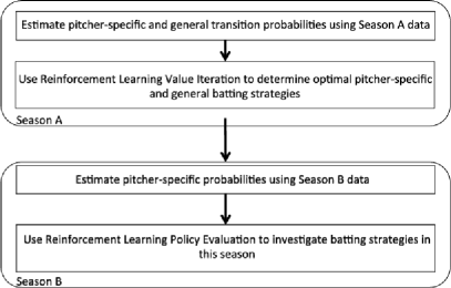
Figure 1: A schematic of the Reinforcement Learning Value Iteration and Policy Evaluation analysis of two seasons of MLB data.

In addition to evaluating the batting strategies on new data, comparison of the performance of the pitcher-specific and general batting strategies yields important information on the utility of an optimal, data-informed batting strategy against a specific pitcher. To this point, a pitcher has been exploited if Policy Evaluation suggests that the pitcher-specific optimal batting strategy against them is superior to the general optimal batting strategy, with their difference or ratio estimating the degree of exploitability. The term “exploited” is used in the sense that an opposing batter would be well served in carefully studying that pitcher’s historical data, rather than executing a general strategy.

Given this framework, it is possible to investigate hypotheses on general pitcher exploitability using permutation tests. However, the nature of the tests requires assumptions on the direction of the alternative. Under the assumption that all pitchers are not equally exploitable, the hypothesis that pitchers can be exploited more than 50% of the time can be investigated. This hypothesis was not rejected at a 5% error rate. Under the assumption that all pitchers are equally exploitable, the hypothesis was rejected. It is our opinion that the assumption of unequal exploitability is better suited for baseball’s at-bat setting (see Section 2.4). Thus, this manuscript is the first to provide statistical evidence in support of strategizing against specific pitchers instead of a group of pitchers.

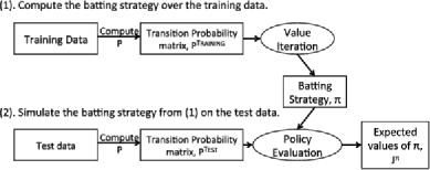
Figure 4: Illustration of the two-stage process of computing and evaluating the batting strategy that is computed over the input training data. This strategy is then given as input, along with the test data’s transition probability matrix $P^{\textsc{\scriptsize Test}}$, to the Policy Evaluation algorithm, which outputs the expected rewards for each state when following batting strategy $\pi$.

To highlight the utility of an optimal pitcher-specific batting strategy for an exploitable pitcher, a data-driven validation was conceived. This validation associates spatial trajectories with the pitch-type that was employed. The spatial component is a classifier that estimates the pitch-type of a batter-parameterized spatial trajectory after training over the respective pitcher’s actual pitch trajectories. The estimated pitch-type selects the batting action from the exploited pitcher’s pitcher-specific batting strategy (Section 4.2; the schematic diagram outlining this process is provided in Figure 4). The simulation therefore uses the spatial and strategic component to realistically simulate a batter’s performance when facing an exploited pitcher. The batter’s actual and simulated statistics when facing the respective pitcher are then compared using typical baseball statistics.

It was found that heuristically-labeled “elite” batters’ simulated statistics are worse than their actual statistics. However, it was also found that the (also heuristically-labeled) “nonelite” batters’ simulated statistics were greatly improved from their actual statistics. The simulation results suggest that an exploited pitcher’s pitcher-specific strategies are useful for nonelite batters.

The manuscript is laid out as follows: The section immediately following this paragraph provides a very brief demonstration of Reinforcement Learning algorithms to help stimulate understanding, Section 2 discusses the strategic component, which applies Reinforcement Learning algorithms to Markov processes to compute and evaluate the respective batting strategies, and Section 3 discusses the spatial component, which simulates a specific batter’s performance using an exploited pitcher’s pitcher-specific batting strategy. Section 4 provides the methodology used to produce the results given in Section 5.

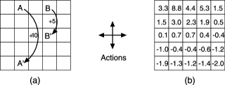
Figure 2: GridWorld. The values in the right grid are determined using Policy Evaluation with a policy that randomly selects one of the four actions at each state. Reprinted with permission from Richard S. Sutton and Andrew G. Barto, Reinforcement Learning: An Introduction, published by The MIT Press.

Reinforcement Learning tutorial

Reinforcement Learning focuses on the problem of decision-making facing uncertainty, which are settings where the decision-maker (agent) interacts with a new, or unfamiliar, environment. The agent continually interacts with the environment by selecting actions, where the environment then responds to these actions and presents new scenarios to the agent [Sutton and Barto (1998)]. This environment also provides rewards, which are numerical values that act as feedback for the action selected by the agent in the environment. At time-unit t, the agent is given the environment’s state $s_{t}\in\mathcal{S}$, and selects action $a_{t}\in\mathcal{A}(s_{t})$, where $\mathcal{A}(s_{t})$ is the set of all possible actions that can be taken at state $s_{t}$. Selecting this action increments the time-unit, giving the agent a reward of $r_{t+1}$ and also causing it to transition to state $s_{t+1}$. Reinforcement Learning methods focus on how the agent changes its decision-making as a consequence of its experiment in the respective environment. The agent’s goal is to use its knowledge of the environment to maximize its reward over the long run. Specifying the environment therefore defines an instance of the Reinforcement Learning problem [Sutton and Barto (1998)] that can be studied further.

GridWorld (Figure 2) is a canonical example that illustrates how Reinforcement Learning algorithms can be applied to various settings. In this example, there are four equiprobable actions that can be taken at each square (state): left, right, up and down, where each action is selected at random Any action taken at either square A or B yields a reward of $+10$ and $+5$, respectively, and transports the user to square A^′ or B^′, respectively. For all other squares, a reward of 0 is given for actions that do not result in falling off the grid, where the latter outcome results in a reward of $-1$.

The negative values in the lower parts of the grid demonstrate that the expected reward of square A is below its immediate reward because after we are transported to square A^′, we are likely to fall off the grid. Conversely, the expected reward of square B is higher than its immediate reward because after we are transported to square B^′, the possibility of running off the grid is compensated for by the possibility of running into square A or B [Sutton and Barto (1998)].

Employing Reinforcement Learning algorithms in various real-world settings allows us to “balance” the immediate and future rewards afforded by the outcomes at each state with their respective probabilities. This approach enables the computation of a sequence of actions, or policy, that maximize the immediate reward while considering the consequences of these actions.

2 Strategic component—Reinforcement Learning in baseball (RLIB)

2.1 Markov processes

Let $\{X^{(t)}\}$ be a Markov process with finite state space ${\mathcal{S}}=\{E_{1},\ldots,E_{n}\}$ where the states represent pitch counts. We assume stationary transition probabilities. That is, $p_{E_{k}\rightarrow E_{j}}=P(X^{(t)}=E_{j}|X^{(t-1)}=E_{k})$ for $E_{j},E_{k}\in{\mathcal{S}}$ is the same for all $t$ [Feller (1968)]. Figure 3 displays the Markov transition diagram omitting the absorbing states (hit, out and walk).

We define optimal policies as a set of actions that maximize the expected reward at every state in a Markov process. Conditioning on a batter’s action at a state yields the probability distribution for the immediate and future state. Since the at-bat always starts from the $s_{0}=\{0,0\}$ state, the long-term reward is defined as

$$J^{*}(s_{0})=\max_{\pi=\{u^{0},\ldots,u^{T}\}}\mathbb{E}\Biggl{\{}\sum_{t=0}^{T}g\bigl{(}s_{t},u^{t},s_{t+1}\bigr{)}\Big{|}s_{0}=\{0,0\},\pi\Biggr{\}},$$ (1)

where:

• $\{s_{t}\}$ is the sequence of states, or pitch counts, in the state space $\mathcal{S}$ visited by the batter for the respective at-bat. We define the set of terminal states—that is, states that conclude the at-bat—as $\mathcal{E}=\{\mathrm{O},\mathrm{S},\mathrm{D},\mathrm{T},\break\mathrm{HR},\mathrm{W}\}\subset\mathcal{S}$, where O, S, D, T, HR, W are abbreviations for Out, Single, Double, Triple, Home Run and Walk, respectively.

• $\pi=\{u^{0},\ldots,u^{T}\}$ is the best batting strategy that contains the batting actions that maximize the expected reward of every state. Since the batter can Swing or Stand at each state, it follows that $u=\mathrm{Swing}$ or $u=\mathrm{Stand}$ for each nonterminal state.

• $g(s_{t},u^{t},s_{t+1})$ is the reward function whose output reflects the batter’s preference of transitioning to state $s_{t+1}$ when selecting the best batting action $u^{t}$ from state $s_{t}$. The reward function used in our study is

  $$g(i,u,j)=\cases{0,&\quad$\mbox{if {j}${}={}$\{O\} or $j\in\mathcal{S}\cap\mathcal{E}^{c}$},$\vspace*{2pt}\cr 1,&\quad$\mbox{if {j}${}={}$\{W\} and {u}${}={}$Stand},$\vspace*{2pt}\cr 2,&\quad$\mbox{if {j}${}={}$\{S\} and {u}${}={}$Swing},$\vspace*{2pt}\cr 3,&\quad$\mbox{if {j}${}={}$\{D\} and {u}${}={}$Swing},$\vspace*{2pt}\cr 4,&\quad$\mbox{if {j}${}={}$\{T\} and {u}${}={}$Swing},$\vspace*{2pt}\cr 5,&\quad$\mbox{if {j}${}={}$ \{HR\} and {u}${}={}$Swing}$}\qquad\forall i\notin\mathcal{E}.$$

  Further information on our formulation of the reward function can be found in Section 5.3.1.

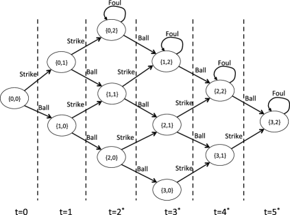
Figure 3: Our view of an at-bat as a Markov process, where each oval denotes the state $\{B,S\}$ in the at-bat, where $B$ and $S$ are the number of balls and strikes, respectively, arrows represent transitions, and $t$ is the time unit that is the number of pitches thrown in the respective at-bat. Asterisks denote that some states at the respective time-unit are still valid transitions at higher time-units—that is, if a batter fouls off a pitch at $t=3$ in the $\{1,2\}$ pitch count, they will still be in this state at $t=4$. We omit the terminal (absorbing) states for neatness.

Equation (1) can be viewed as the maximized expected reward of state $\{0,0\}$ when following batting strategy $\pi$, which is comprised of actions that maximize the expected reward over all of the at-bats $\{s_{t}\}$ given as input [Bertsekas and Tsitsiklis (1996)].

To find the batting actions that comprise the best batting strategy, we find the batting action $u$ that satisfies the optimal expected reward function for state $i$ [Bertsekas and Tsitsiklis (1996)]:

$$J^{*}(i)=\max_{u\in U}\biggl{[}\sum_{j\in\mathcal{S}}P_{u}^{\textsc{\scriptsize{Training}}}(i,j)\bigl{(}g(i,u,j)+J^{*}(j)\bigr{)}\biggr{]}\qquad\forall i\in\mathcal{S}\cap\mathcal{E}^{c},$$ (2)

where $P_{u}^{\textsc{\scriptsize Training}}(i,j)$ is an estimated probability of transitioning from state i to j when selecting batting action u on the pitch-by-pitch data and $J^{*}(i)$ is the maximized expected reward of state $i$ when selecting the action $u$ that achieves this maximum.

The Value Iteration algorithm, shown in Figure 5, solves for the batting actions that satisfy equation (2). Intuitively, the algorithm keeps iterating until the state’s reward function is close to its optimal reward function $J^{*}$, where in the limit $J^{*}=\lim_{k\to\infty}J^{k}(i)\ \forall i\in\mathcal{S}$ [Patek and Bertsekas (1996)]. The algorithm terminates upon satisfying the convergence criterion $\Delta<\varepsilon$, where $\varepsilon=2.22\times 10^{-16}$ is the machine-epsilon predefined in the MATLAB programming language; this epsilon ensures that the reward functions of each state have approximately 15–16 digits of precision.

The Policy Evaluation algorithm, shown in Figure 6, uses the best batting strategy $\pi$ on a different season of the respective pitcher’s pitch-by-pitch data to calculate the expected reward of each state in the at-bat, given by

$$J^{\pi}(i)=\sum_{j\in\mathcal{S}}P_{\pi(i)}^{\textsc{\scriptsize Test}}(i,j)\bigl{[}g\bigl{(}i,\pi(i),j\bigr{)}+J^{\pi}(j)\bigr{]}\qquad\forall i\in\mathcal{S}\cap\mathcal{E}^{c},$$ (3)

where $J^{\pi}(i)$ is the expected reward of state $i$ when following the batting strategy $\pi$.

[ruled]Value IterationP^Training,g,S, U Δ= 0
i ∈S∩E^c
    v ←J(i)
    J(i) ←max_u ∑_j P_u^Training(i,j)[g(i,u,j) + J(j)]
    Δ←max(Δ, —v - J(i)—)
(Δ¡ ε)
deterministic policy  π= {u^0, …, u^n-1}

Figure 5: The Value Iteration algorithm outputs the batting strategy $\pi$ that maximizes the expectation at each state over the input data. Reprinted with permission from Richard S. Sutton and Andrew G. Barto, Reinforcement Learning: An Introduction, published by The MIT Press.

[ruled]Policy EvaluationP^Test,g,S, π Δ= 0
i ∈S∩E^c
   v ←J(i)
   J(i) ←∑_j P_π(i)^Test(i,j) [g(i,π(i),j) + J(j)]
   Δ←max(Δ, —v - J(i)—)
(Δ¡ ε)
J^π

Figure 6: The Policy Evaluation algorithm, that calculates the expected rewards of every state when using the batting strategy $\pi$, given by $J^{\pi}\in\mathbb{R}^{n}$, on the input data. Reprinted with permission from Richard S. Sutton and Andrew G. Barto, Reinforcement Learning: An Introduction, published by The MIT Press.

The transition probability matrices estimated via the training and test data, represented by $P_{u}^{\textsc{\scriptsize Training}}(i,j)$ and $P_{u}^{\textsc{\scriptsize Test}}(i,j)$ in equations (2) and (3), respectively, are the transition probabilities used by Value Iteration and Policy Evaluation to compute and evaluate, respectively, the best batting strategy, $\pi$. The batting strategies are estimated against probability transitions matrices computed from either a population of at-bats for one season of a single pitcher’s data (pitcher-specific batting strategy) or one season of a population of pitchers’ data (general batting strategy; see Section 4.1).

Policy Evaluation therefore allows a quantitative comparison of the pitcher-specific and general batting strategies, $\pi^{p}$ and $\pi^{g}$, on the same transition probabilities representing the pitcher’s decision-making. Equation (3) shows that the $\{0,0\}$ state’s expected reward, denoted by $J(\{0,0\})$, requires the expected reward of every other state to be calculated first. It follows that $J(\{0,0\})$ is the expected reward of the entire at-bat. Thus, a pitcher is exploited if and only if $J^{\pi^{p}}(\{0,0\})\geq J^{\pi^{g}}(\{0,0\})$ [Sutton and Barto (1998)] (see Section 2.4).

2.2 Models

The generality of the Markov process allows us to propose models with various degrees of resolution, which depends on the number of phenomena considered at each state. Below we outline two models of information resolution as useful starting points.

2.2.1 Simple RLIB (SRLIB)

Initially, we represented a pitcher’s decisions by conditioning the pitch outcome (reflected by the future pitch count) on the batter’s action at the previous pitch count. SRLIB therefore has $n=|\mathcal{S}_{S}\cap\mathcal{E}^{c}|=12$ nonterminal states

$$\mathcal{S}_{S} = \bigl{\{}\{0,0\},\{1,0\},\{2,0\},\{3,0\},\{0,1\},\{0,2\},\{1,1\},\{1,2\},\{2,1\},\{2,2\},$$

$$\hskip 157.0pt\{3,1\},\{3,2\},\mathrm{O},\mathrm{S},\mathrm{D},\mathrm{T},\mathrm{HR},\mathrm{W}\bigr{\}}.$$

2.2.2 Complex RLIB (CRLIB)

CRLIB conditions the pitcher’s selected pitch-type at the current pitch count on both the pitch-type and batting actions at the previous pitch count.

We observed that the MLB GameDay system gave as many as 8 pitch-types for one pitcher. We therefore generalized pitch-types to four categories: fastball-type, curveball/changeup, sinking/sliding, and knuckleball/unknown pitches. Assuming the set of pitch-types is $\mathcal{T}$, our abstraction admits at most four pitch-types for every pitcher—that is, $|\mathcal{T}|\leq 4$.

The inclusion of pitch-types results in state space $\mathcal{S}_{C}=\{\mathcal{S}_{S}\cap\mathcal{E}^{c}\}\times\mathcal{T}\cup\mathcal{E}$, where every nonterminal state incorporates the four pitch-types at each pitch count, giving $n=|\{\mathcal{S}_{S}\cap\mathcal{E}^{c}\}\times\mathcal{T}|=48$ nonterminal states,

$$\mathcal{S}_{C} = \bigl{\{}\{0,0\},\{1,0\},\{2,0\},\{3,0\},\{0,1\},\{0,2\},\{1,1\},\{1,2\},\{2,1\},\{2,2\},$$

$$\hskip 243.0pt\{3,1\},\{3,2\}\bigr{\}}$$

$${}\times\mathcal{T}\cup\mathcal{E}.$$

We represent the expected reward of the $\{0,0\}$ state as the weighted average over the expected rewards of the four pitch types associated with the $\{0,0\}$ state:

$$J^{\pi}\bigl{(}\{0,0\}\bigr{)}=\frac{1}{K}\sum_{t_{i}\in\mathcal{T}}K_{t_{i}}J^{\pi}\bigl{(}\{0,0\}\times t_{i}\bigr{)},$$

where $K_{t_{i}}$ is the number of times pitch-type $t_{i}$ was thrown in the test data and $K$ is the total number of pitches in the test data.

$\pi_{\mathrm{SRLIB}}^{p}=\left[\matrix{\{0,0\}\vspace*{2pt}\cr\{1,0\}\vspace*{2pt}\cr\{2,0\}\vspace*{2pt}\cr\{3,0\}\vspace*{2pt}\cr\{0,1\}\vspace*{2pt}\cr\{0,2\}\vspace*{2pt}\cr\{1,1\}\vspace*{2pt}\cr\{1,2\}\vspace*{2pt}\cr\{2,1\}\vspace*{2pt}\cr\{2,2\}\vspace*{2pt}\cr\{3,1\}\vspace*{2pt}\cr\{3,2\}}\right]=\left[\matrix{0\vspace*{2pt}\cr 1\vspace*{2pt}\cr 0\vspace*{2pt}\cr 0\vspace*{2pt}\cr 0\vspace*{2pt}\cr 0\vspace*{2pt}\cr 0\vspace*{2pt}\cr 0\vspace*{2pt}\cr 1\vspace*{2pt}\cr 0\vspace*{2pt}\cr 0\vspace*{2pt}\cr 0}\right]$

$\pi_{\mathrm{CRLIB}}^{p}=\left[\matrix{\left[\matrix{0&1&0&0&0&1&0&0&0&1&0&0}\right]^{\top}\vspace*{2pt}\cr[\mathrm{null}]^{\top}\vspace*{2pt}\cr\left[\matrix{0&0&1&1&1&0&0&0&1&0&1&0}\right]^{\top}\vspace*{2pt}\cr[\mathrm{null}]^{\top}}\right]$

$\pi_{\mathrm{SRLIB}}^{g}=\left[\matrix{\{0,0\}\vspace*{2pt}\cr\{1,0\}\vspace*{2pt}\cr\{2,0\}\vspace*{2pt}\cr\{3,0\}\vspace*{2pt}\cr\{0,1\}\vspace*{2pt}\cr\{0,2\}\vspace*{2pt}\cr\{1,1\}\vspace*{2pt}\cr\{1,2\}\vspace*{2pt}\cr\{2,1\}\vspace*{2pt}\cr\{2,2\}\vspace*{2pt}\cr\{3,1\}\vspace*{2pt}\cr\{3,2\}}\right]=\left[\matrix{0\vspace*{2pt}\cr 0\vspace*{2pt}\cr 1\vspace*{2pt}\cr 1\vspace*{2pt}\cr 0\vspace*{2pt}\cr 0\vspace*{2pt}\cr 0\vspace*{2pt}\cr 0\vspace*{2pt}\cr 0\vspace*{2pt}\cr 0\vspace*{2pt}\cr 0\vspace*{2pt}\cr 0}\right]$

$\pi_{\mathrm{CRLIB}}^{g}=\left[\matrix{\left[\matrix{0&0&1&0&1&0&1&0&1&0&1&1}\right]^{\top}\vspace*{2pt}\cr\left[\matrix{0&0&0&1&0&0&1&1&1&0&1&1}\right]^{\top}\vspace*{2pt}\cr\left[\matrix{0&0&0&0&0&0&1&0&1&1&1&1}\right]^{\top}\vspace*{2pt}\cr[\mathrm{null}]^{\top}}\right]$

Figure 7: The pitcher-specific and general strategies, denoted by $\pi^{p}$ and $\pi^{g}$, respectively, computed on SRLIB and CRLIB for the 2009 season. CRLIB’s pitcher-specific batting strategy for Roy Halladay had an empty second and fourth row because the MLB GameDay system reported he did not throw any Sinking/sliding or Knuckleball/unknown type pitches in the training data; a similar argument holds for the general batting strategy’s fourth row.

2.3 Illustration of batting strategies

We now illustrate the batting strategies that are produced by either SRLIB or CRLIB, respectively. As shown in Figure 7, SRLIB and CRLIB have n-dimensional and ($n\times 4$)-dimensional batting strategies, respectively. The action at each state is represented by a binary value corresponding to Stand (0) and Swing (1).

For the strategies given in Figure 7, CRLIB/SRLIB’s pitcher-specific batting strategy exploited Roy Halladay on the 2010 test data. However, only CRLIB exploits Halladay on the 2008 test data, presumably because it incorporates information about his pitch selection, as it is believed that pitchers often rely on their “best pitches” in specific pitch counts. For example: If Halladay throws a fastball in the $\{2,2\}$ pitch count, $\pi^{p}_{\mathrm{SRLIB}}$ selects the batting action $u=\operatorname{Stand}$, whereas $\pi^{p}_{\mathrm{CRLIB}}$ selects $u=\operatorname{Swing}$. In comparison to the SRLIB model, we see that the inclusion of pitch type gives the CRLIB model an enriched representation that can improve a batter’s opportunity of reaching base.

2.4 Comparing an “intuitive” and general batting strategy

We show that the general batting strategy is a more competitive baseline performance measure than an intuitive batting strategy. This intuitive batting strategy selects the action Swing at states $\{1,0\},\{2,0\},\{3,0\},\{2,1\},\{3,1\}$, and Stand in states $\{0,0\},\{1,1\},\{1,2\},\{2,2\},\{3,2\},\{0,1\},\{0,2\}$. In other words, the intuitive batting strategy reflects the intuition that the batter should only swing in a batter’s count; we show that these types of batting strategies are inferior to statistically computed ones, such as the general batting strategy.

After performing Policy Evaluation for both batting strategies, we observed that the general batting strategy outperformed the intuitive batting strategy 146 out of 150 times. The general batting strategy’s dominant performance justifies its selection as the competitive baseline performance measure. Thus, we cannot assume that the pitcher-specific batting strategy will perform better than, or even equal to, the general batting strategy when performing Policy Evaluation on the respective pitcher’s test data.

Since each pitcher’s “best pitch(es)” can vary, it follows that the probability distributions over future states from the current state will also vary, especially in states with a batter’s count. This is a consequence of the uniqueness of each pitcher’s behaviour, which is reflected through their pitch selection at each state in the at-bat, and thereby quantified in their respective transition probabilities. This is personified by R. A. Dickey, as he only has one “best pitch” (knuckleball) and throws other pitch types to make his behaviour less predictable. Thus, when Dickey’s knuckleball is ineffective, an optimal policy will recommend swinging at every nonknuckle pitch, as it is computed over data that shows an improved outcome for the batter. In contrast, pitchers that consistently throw more than one pitch type for strikes, such as Roy Halladay, are more difficult to exploit via the pitcher-specific batting strategy because the improved outcome in swinging at their “weaker” pitches is marginal in comparison to pitchers that consistently throw fewer pitch types for strikes. Given that the pitcher-specific and general batting strategies are computed over different populations, and each at-bat contains information about the respective pitcher’s behaviour, it follows that pitchers are not equally susceptible to being exploited in an empirical setting.

If the pitcher-specific batting strategy performs equal to the general batting strategy, the competitiveness/dominance of the latter over intuitively-constructed batting strategies ensures that the respective pitcher is still exploited because the intuitive batting strategy can be viewed as the standard strategy that is employed in baseball. Let $\pi^{i}$ be the intuitive batting strategy and assume that the pitcher-specific batting strategy performs equal to the general batting strategy. By transitivity, $J^{\pi^{g}}(\{0,0\})\gg J^{\pi^{i}}(\{0,0\})$, and $J^{\pi^{p}}(\{0,0\})==J^{\pi^{g}}(\{0,0\})$, then $J^{\pi^{p}}(\{0,0\})\gg J^{\pi^{i}}(\{0,0\})$.

3 Spatial component

A spatial component is introduced to highlight the utility of the exploited pitchers’ pitcher-specific batting strategies. The spatial component associates the pitch-type based on the respective pitch’s spatial trajectory, where this trajectory is parameterized specifically to the batter being simulated. Thus, the spatial component predicts the pitch-type for the batter-parameterized spatial trajectory given as input. This allows us to simulate a batter’s performance when they use the exploited pitcher’s pitcher-specific batting strategy against the respective pitcher (see Figure 9).

The spatial information for each pitch contains the three-dimensional acceleration, velocity, starting and ending positions. This information is obtained from the MLB GameDay system after it fits a quadratic polynomial to 27 instantaneous images representing the pitch’s spatial trajectory. These pictures are taken by cameras on opposite sides of the field. The MLB GameDay system therefore performs a quadratic fit to the trajectory data.

There are two problems with this fit. First, acceleration is assumed to be constant, which is certainly not true. Second, there exists a near-perfect correlation between variables obtained from the fit (such as velocity and the end location of a pitch) and the independent variable (acceleration) used to produce this fit. Figure 8 displays pitch locations along with predicted values from regression with velocity or acceleration as predictors and location as the response.

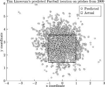
Figure 8: The actual (square) and predicted (circle) locations for Tim Lincecum’s pitches in the 2009 season, when performing OLS regression on break angle, initial velocity, and break length features to predict the end location of each pitch. The rectangle in the center of the plot represents the strike zone.

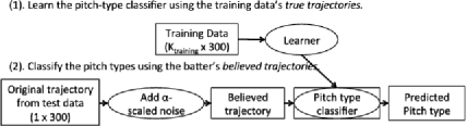
Figure 9: Illustrating our spatial model, where $\alpha$ is parameterized according to the batter, $K_{\mathrm{training}}$ denotes the number of pitches in the respective pitcher’s training data, and 300 represents the $m=100$ three-dimensional points that describe the pitch trajectory. Here, the Learner is a quadratic kernel Support Vector Machine (SVM).

We see that the quadratic fit severely limits the use of each pitch’s spatial trajectory. To address this limitation, we use the instantaneous positions of every pitch trajectory to predict the pitch type.

3.1 Batter-parameterized pitch identification

We add $\alpha$-scaled noise, where $\alpha$ is a batter-specific parameter, to the original spatial trajectory of each pitch to represent the respective batter’s believed trajectories. This is achieved by first drawing independent, identically distributed noise from the uniform distribution on the $[-1,1]$ interval, which is then multiplied by the parameter $\alpha$, and finally added to the m evenly-spaced, three-dimensional, instantaneous positions of the original (true) pitch trajectory.

For the batter’s believed trajectories to accurately represent their pitch-identification ability, $\alpha$ is defined as the number of strikeouts divided by the number of plate appearances on the same year which the batting strategy is computed on. Only considering strikeouts is justified by the fact that any recorded out from putting the ball in play implies that a player identified the ball accurately enough to achieve contact. In contrast, a batter that strikes out either failed to identify the pitch as a strike or failed to establish contact with the ball. Thus, adding $\alpha$-scaled noise to original trajectory reproduces a batter’s believed trajectory.

The training data’s true trajectories are given as input to a Support Vector Machine (SVM) [Vapnik (1998), Hastie, Tibshirani and Friedman (2009)] with a quadratic kernel, where each trajectory’s $m=100$ three-dimensional instantaneous positions form a single data point that has an associated pitch-type. The SVM algorithm then computes a spatial classifier, which is composed of coefficients $\bolds\beta=[\beta_{0},\ldots,\beta_{300}]$, that best separates the training data’s original trajectories according to pitch-type, usually with high accuracy.

= 2008 2009 2010 Player ERA WHIP W L IP ERA WHIP W L IP ERA WHIP W L IP Roy Halladay $2.78$ $1.053$ $20$ $11$ $246.0$ $2.79$ $1.126$ $17$ $10$ $239.0$ $2.44$ $1.041$ $21$ $10$ $250.2$ Cliff Lee $2.54$ $1.110$ $22$ $3$ $223.1$ $3.22$ $1.243$ $14$ $13$ $231.2$ $3.18$ $1.003$ $12$ $9$ $212.1$ Cole Hamels $3.09$ $1.082$ $14$ $10$ $227.1$ $4.32$ $1.286$ $10$ $11$ $193.2$ $3.06$ $1.179$ $12$ $11$ $208.2$ Jon Lester $3.21$ $1.274$ $16$ $6$ $210.1$ $3.41$ $1.230$ $15$ $8$ $203.1$ $3.25$ $1.202$ $19$ $9$ $208.0$ Zack Greinke $3.47$ $1.275$ $13$ $10$ $202.1$ $2.16$ $1.073$ $16$ $8$ $229.1$ $4.17$ $1.245$ $10$ $14$ $220.0$ Tim Lincecum $2.62$ $1.172$ $18$ $5$ $227.0$ $2.48$ $1.047$ $15$ $7$ $225.1$ $3.43$ $1.272$ $16$ $10$ $212.1$ CC Sabathia $2.70$ $1.115$ $17$ $10$ $253.0$ $3.37$ $1.148$ $19$ $8$ $230.0$ $3.18$ $1.191$ $21$ $7$ $237.2$ Johan Santana $2.53$ $1.148$ $16$ $7$ $234.1$ $3.13$ $1.212$ $13$ $9$ $166.2$ $2.98$ $1.170$ $11$ $9$ $199.0$ Felix Hernandez $3.45$ $1.385$ $9$ $11$ $200.2$ $2.49$ $1.135$ $19$ $5$ $238.8$ $2.27$ $1.057$ $13$ $12$ $249.2$ Chad Billingsley $3.14$ $1.336$ $16$ $10$ $200.2$ $4.03$ $1.319$ $12$ $11$ $196.1$ $3.57$ $1.278$ $12$ $11$ $191.2$ Jered Weaver $4.33$ $1.285$ $11$ $10$ $176.2$ $3.75$ $1.242$ $16$ $8$ $211.0$ $3.01$ $1.074$ $13$ $12$ $224.1$ Clayton Kershaw $4.26$ $1.495$ $5$ $5$ $107.2$ $2.79$ $1.229$ $8$ $8$ $171.0$ $2.91$ $1.179$ $13$ $10$ $204.1$ Chris Carpenter $1.76$ $1.304$ $0$ $1$ $15.1$ $2.24$ $1.007$ $17$ $4$ $192.2$ $3.22$ $1.179$ $16$ $9$ $235.0$ Matt Garza $3.70$ $1.240$ $11$ $9$ $184.2$ $3.95$ $1.261$ $8$ $12$ $203.0$ $3.91$ $1.251$ $15$ $10$ $204.2$ Adam Wainwright $3.20$ $1.182$ $11$ $3$ $132.0$ $2.63$ $1.210$ $19$ $8$ $233.0$ $2.42$ $1.051$ $20$ $11$ $230.1$ Ubaldo Jimenez $3.99$ $1.435$ $12$ $12$ $198.2$ $3.47$ $1.229$ $15$ $12$ $218.0$ $2.88$ $1.155$ $19$ $8$ $221.2$ Matt Cain $3.76$ $1.364$ $8$ $14$ $217.2$ $2.89$ $1.181$ $14$ $8$ $217.2$ $3.14$ $1.084$ $13$ $11$ $223.1$ Jonathan Sanchez $5.01$ $1.449$ $9$ $12$ $158.0$ $4.24$ $1.365$ $8$ $12$ $163.1$ $3.07$ $1.231$ $13$ $9$ $193.1$ Roy Oswalt $3.54$ $1.179$ $17$ $10$ $208.2$ $4.12$ $1.241$ $8$ $6$ $181.1$ $2.76$ $1.025$ $13$ $13$ $211.2$ Justin Verlander $4.84$ $1.403$ $11$ $17$ $201.0$ $3.45$ $1.175$ $19$ $9$ $240.0$ $3.37$ $1.163$ $18$ $9$ $224.1$ Josh Johnson $3.61$ $1.351$ $7$ $1$ $87.1$ $3.23$ $1.158$ $15$ $5$ $209.0$ $2.30$ $1.105$ $11$ $6$ $183.2$ John Danks $3.32$ $1.226$ $12$ $9$ $195.0$ $3.77$ $1.283$ $13$ $11$ $200.1$ $3.72$ $1.216$ $15$ $11$ $213.0$ Edwin Jackson $4.42$ $1.505$ $14$ $11$ $183.1$ $3.62$ $1.262$ $13$ $9$ $214.0$ $4.47$ $1.395$ $10$ $12$ $209.1$ Max Scherzer $3.05$ $1.232$ $0$ $4$ $56.0$ $4.12$ $1.344$ $9$ $11$ $170.1$ $3.50$ $1.247$ $12$ $11$ $195.2$ Ted Lilly $4.09$ $1.226$ $17$ $9$ $204.2$ $3.10$ $1.056$ $12$ $9$ $177.0$ $3.62$ $1.079$ $10$ $12$ $193.2$ [*]ttl1Please see Appendix for baseball terminology.

Table 1: The annual statistics from the 2008, 2009 and 2010 seasons for the 25 pitchers used in our evaluation[*]ttl1

The spatial classifier allows pitch-type identification to be standardized across batters, because the respective batter’s believed trajectory is only identified as the correct pitch-type if it is similar to the original trajectory. If the believed trajectory differs enough from the original trajectory, it will be identified as the incorrect pitch-type; this is reflective of players with higher $\alpha$ values that strike out often. We can therefore view the spatial classifier as an oracle.

4 Methods and evaluation

4.1 Strategic component

For our evaluation, we use 3 years of pitch-by-pitch data for 25 elite pitchers, as shown in Table 1. We evaluated the batting strategies performance for all six unique combinations of the training and test data, which gave a total of $25\times 6=150$ pitcher-specific batting strategies. The data was obtained from MLB’s GameDay system, which provided three complete seasons of pitching data, containing the pitch outcome, pitch-type, number of balls and strikes, and the batter’s actions. The technical details of the data collection and formatting process, which is necessary before applying the Reinforcement Learning algorithms, are provided in the supplement [Sidhu and Caffo (2014)].

Initially the general batting strategy was trained over all pitchers data for the respective season, where it was observed that the general batting strategy outperformed the pitcher-specific batting strategies on the respective season by a significant margin. In other words, training the general batting strategy over all of the pitchers’ annual data led to invalidation of the hypothesis, regardless of whether pitchers were equally exploitable. Given that the general batting strategy was trained over a much larger data set than the pitcher-specific batting strategy, we sought a way to standardize the training data used to compute the general batting strategy, which is described in the following paragraph. We acknowledge that in real-world settings, each of the batting strategies should be trained over all available information, as this information improves the resolution and precision of the probability estimates exploited by the batting strategy.

The size of the general batting strategy’s training data is approximately equal to the average number of pitches thrown by the 25 pitchers in the respective season, where every pitcher’s at-bats in this data set were randomly sampled from all of their at-bats for the respective season. To ensure the general batting strategy’s training data is representative of all pitchers’ data for the respective season, sampling terminates after adding an at-bat for which the total number of pitches exceeds the proportion of pitches that should be contributed by the pitcher. For example, Roy Halladay threw 3319 pitches in 2009, and all 25 pitchers threw a total of 80,879 pitches. Roy Halladay therefore contributes $\lceil{0.04103\times 3235.16}\rceil=133$ pitches to the data set. Repeating this process for all 25 pitchers 2009 data gives a data set comprised of 3276 pitches.

To address the possibility that the aggregate data sample contains unrepresentative at-bats for pitcher(s), which would misrepresent the performance of the general batting strategy, the aggregate data sample was independently constructed 10 times, where the general batting strategy was computed against each of the 10 (training) data samples. Thus, the general batting strategy performance is the average over the 10 general batting strategies’ expected rewards on the test data.

We evaluate the hypothesis under two different assumptions: all pitchers are equally susceptible to being exploited, and all pitchers are not equally susceptible to being exploited, where we believe the latter assumption is more relevant to the real-world setting (see Section 2.4 for our explanation). The null hypothesis is the same under either assumption, but the alternative hypothesis $H_{1}$ is slightly different:

$p=\frac{1}{2}$. The pitcher-specific and general batting strategy are equally likely to exploit the respective pitcher.

$p>\frac{1}{2}$. The pitcher-specific batting strategy will perform:

1. [ ]

2. strictly better than the general batting strategy more than 50% of the time (assuming that pitchers are equally exploitable).

3. better than or equal to the general batting strategy more than 50% of the time (assuming that pitchers are not equally exploitable).

For both hypotheses, the p-value calculation is given by

$$P(X>M)=\sum_{i=M+1}^{150}\pmatrix{150\cr i}p^{i}(1-p)^{150-i},$$

where M is the number of pitcher-specific batting strategies that exploit the respective pitcher(s). Under the assumption that the pitchers are equally exploitable, $H_{0}$ could not be rejected; when assuming that pitchers are not equally exploitable, $H_{0}$ was rejected only for the CRLIB model ($P(X>M)=3e\mbox{--}2$, $M=87$).

When Policy Evaluation is performed on the pitcher-specific or general batting strategy, the pitch-type thrown at the current pitch count is given before selecting the batting action. It follows that Policy Evaluation implicitly assumes that the pitch-types are always identified correctly. This was a desirable assumption because it only considers the strategic aspect of the at-bat when calculating the expected rewards for the respective strategy. It follows that the hypothesis evaluation is completely independent of the batters used in the evaluation.

4.2 Simulating batting strategies with the spatial component

We define the chance threshold as the proportion of the majority pitch-type thrown in the training data, which serves as a baseline for a batter’s pitch-type identification ability. We only simulate batters whose believed trajectories from the test data are classified with an accuracy above the chance threshold. This stipulation reflects our requirement that a batter must be able to identify pitch-types better than guessing the majority pitch-type. Table 2 provides the classification accuracies for the batters included in our simulation.

= Accuracy Batter Pitcher $\bolds{\alpha}$ Training Test Chance threshold # of PA (in 2009) Miguel Cabrera Zack Greinke 0.1466 $2776/2903$ (95.63%) $3135/3376$ (92.86%) $2005/3376$ (59.39%) 14 Joey Votto Roy Oswalt 0.1929 $3050/3374$ (90.4%) $1926/3151$ (61.12%) $1787/3151$ (56.71%) 12 Joe Mauer Justin Verlander 0.0908 $3545/3633$ (97.58%) $3664/3794$ (96.57%) $2553/3794$ (67.29%) 14 Ichiro Suzuki CC Sabathia 0.1175 $3154/3736$ (84.42%) $3089/3985$ (71.86%) $2405/3095$ (54.99%) 11 Jose Bautista Jon Lester 0.1698 $3047/3263$ (93.38%) $2486/3397$ (73.18%) $2423/3397$ (71.33%) 11 Derek Jeter Matt Garza 0.1434 $3201/3331$ (96.1%) $3125/3288$ (95.04%) $2336/3288$ (71.05%) 14 Prince Fielder Matt Cain 0.1933 $3265/3782$ (95.85%) $3019/3177$ (95.03%) $1986/3177$ (62.51%) 09 Matt Holliday Clayton Kershaw 0.1378 3291/3328 (98.89%) 2872/3062 (93.79%) 2163/3062 (70.64%) 08 Ryan Howard Tim Lincecum 0.2532 $3633/3870$ (93.88%) $3047/3338$ (91.28%) $1874/3338$ (56.14%) 07 Mark Teixeira Cliff Lee 0.1713 $3292/3427$ (96.06%) $3134/3965$ (79.04%) $2542/3965$ (64.11%) 14 Nick Markakis Jon Lester 0.1311 $3047/3263$ (93.38%) $2475/3397$ (72.86%) $2423/3397$ (71.33%) 13 Carlos Gonzalez Matt Cain 0.2123 $3265/3782$ (95.85%) $3008/3177$ (94.68%) $1986/3177$ (62.51%) 07 Evan Longoria Roy Halladay 0.1876 $3712/3782$ (98.15%) $3146/3319$ (94.79%) $2445/3319$ (73.67%) 23 Brandon Philips Chris Carpenter 0.1208 $2884/3420$ (84.33%) $1438/2623$ (54.82%) $1227/2623$ (46.78%) 11 Manny Ramirez Jonathan Sanchez 0.1879 $3420/3529$ (96.91%) $2391/2724$ (87.78%) $1866/2724$ (68.50%) 11 Adrian Gonzalez Matt Cain 0.1645 $3265/3782$ (95.85%) $3042/3177$ (95.75%) $1986/3177$ (62.51%) 07 Carl Crawford CC Sabathia 0.1569 $3154/3736$ (84.42%) $3061/3985$ (76.81%) $2405/3985$ (60.35%) 13 Troy Tulowitzki Clayton Kershaw 0.1475 $3291/3328$ (98.89%) $2883/3062$ (94.15%) $2163/3062$ (70.64%) 14 Matt Kemp Jonathan Sanchez 0.2545 $3420/3529$ (96.91%) $2394/2724$ (87.89%) $1866/2724$ (68.50%) 11 Alex Rodriguez Roy Halladay 0.1647 $3712/3782$ (98.15%) $3147/3319$ (94.82%) $2445/3319$ (73.67%) 18 [*]ttl2Please see Appendix for baseball terminology.

Table 2: Evaluating the pitch identification ability on the 2009 (test) data, after training the spatial classifier on 2010 data. The accuracy is the number of correctly predicted pitch-types on the respective batter’s believed trajectories from the 2009 season, after only observing the original trajectories from 2010. The chance threshold is provided to show “how much better” the batter is doing than blindly guessing one class[*]ttl2

We use the spatial component to evaluate twenty prominent batters. Among these batters, ten are considered elite and ten are considered to be nonelite. We simulate each batter’s performance against an exploited pitcher when using the respective pitcher-specific batting strategy. For every at-bat that is simulated, the spatial component first predicts the pitch-type using the respective batter’s believed trajectory. Then, this predicted pitch-type is used with the current state to select the appropriate action from the pitcher-specific batting strategy; see Figure 10.

After identifying the pitch-type and selecting the batting action, the conditional distribution over the future states in the at-bat becomes determined. We assign the future states “bin” lengths that are equal to the probability of transitioning to their respective states, where each bin is a disjoint subinterval on [0,1]. We then generate a random value from the uniform distribution on the [0,1] interval and select the future state whose subinterval contains this random value. To ensure that the performance of the batter versus pitcher is representative of each state’s distribution over future states, every at-bat is simulated 100 times.

5 Results

5.1 Strategic component

The number of pitcher-specific batting strategies that exploited the respective pitcher are given in Table 3. The raw results for SRLIB/CRLIB are given in Tables 4 and 5, respectively.

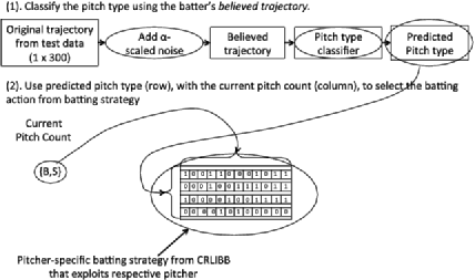
Figure 10: Illustrating the simulation for a batter using an exploited pitcher’s pitcher-specific batting strategy. The spatial classifier’s predicted pitch-type is used to select the row that contains the batting actions for the respective pitch-type, and the current pitch count is used to select the batting action for this pitch-type.

Table 3: The number of exploited pitchers using the respective train/test data partitions

	Year of computed batting strategy
Model	2008		2009		2010
	2009	2010	2008	2010	2008	2009
SRLIB	11	10	5	12	11	14
CRLIB	12	15	11	16	16	16

= Training on 2008 data Training on 2009 data Training on 2010 data 2009 2010 2008 2010 2008 2009 Player $\bolds{J^{\pi^{g}}}$ $\bolds{J^{\pi^{p}}}$ $\bolds{J^{\pi^{g}}}$ $\bolds{J^{\pi^{p}}}$ $\bolds{J^{\pi^{g}}}$ $\bolds{J^{\pi^{p}}}$ $\bolds{J^{\pi^{g}}}$ $\bolds{J^{\pi^{p}}}$ $\bolds{J^{\pi^{g}}}$ $\bolds{J^{\pi^{p}}}$ $\bolds{J^{\pi^{g}}}$ $\bolds{J^{\pi^{p}}}$ Roy Halladay 0.655 0.604 0.546 0.491 0.659 0.569 0.569 $\mathbf{0.766}$ 0.699 0.560 0.638 $\mathbf{0.707}$ Cliff Lee 0.692 $\mathbf{0.706}$ 0.566 $\mathbf{0.622}$ 0.680 0.622 0.558 0.499 0.678 0.664 0.707 0.571 Cole Hamels 0.716 $\mathbf{0.768}$ 0.814 0.795 0.731 0.700 0.807 0.764 0.724 0.719 0.700 0.680 Jon Lester 0.713 $\mathbf{0.764}$ 0.876 0.847 0.742 0.737 0.831 0.718 0.739 $\mathbf{0.741}$ 0.710 0.709 Zack Greinke 0.642 0.608 0.747 $\mathbf{0.835}$ 0.795 0.688 0.739 0.719 0.824 $\mathbf{0.836}$ 0.607 $\mathbf{0.672}$ Tim Lincecum 0.649 $\mathbf{0.694}$ 0.822 0.785 0.717 0.694 0.778 0.723 0.686 0.589 0.653 0.565 CC Sabathia 0.810 0.718 0.802 0.698 0.657 0.550 0.792 $\mathbf{0.821}$ 0.593 0.550 0.825 $\mathbf{0.836}$ Johan Santana 0.785 $\mathbf{0.862}$ 0.773 0.703 0.680 $\mathbf{0.694}$ 0.774 $\mathbf{0.838}$ 0.651 $\mathbf{0.773}$ 0.744 $\mathbf{0.852}$ Felix Hernandez 0.721 $\mathbf{0.784}$ 0.823 0.786 0.777 0.765 0.815 0.786 0.717 0.662 0.760 0.613 Chad Billingsley 0.802 $\mathbf{0.865}$ 0.788 $\mathbf{0.812}$ 0.750 $\mathbf{0.790}$ 0.792 $\mathbf{0.812}$ 0.752 $\mathbf{0.785}$ 0.792 $\mathbf{0.860}$ Jered Weaver 0.860 0.841 0.691 $\mathbf{0.734}$ 0.762 $\mathbf{0.770}$ 0.704 $\mathbf{0.711}$ 0.770 0.759 0.883 0.840 Clayton Kershaw 0.738 0.719 0.716 0.667 0.909 $\mathbf{1.125}$ 0.710 0.691 0.996 0.800 0.757 $\mathbf{0.837}$ Chris Carpenter 0.751 0.640 0.691 $\mathbf{0.732}$ 0.757 0.692 0.753 $\mathbf{0.791}$ 0.667 $\mathbf{0.944}$ 0.809 $\mathbf{0.914}$ Matt Garza 0.827 0.792 0.794 $\mathbf{0.794}$ 0.725 0.622 0.779 $\mathbf{0.834}$ 0.692 0.622 0.797 $\mathbf{0.880}$ Adam Wainwright 0.689 $\mathbf{0.690}$ 0.692 0.648 0.609 0.578 0.694 $\mathbf{0.738}$ 0.554 $\mathbf{0.636}$ 0.707 0.705 Ubaldo Jimenez 0.735 0.709 0.767 $\mathbf{0.771}$ 0.867 0.850 0.751 0.741 0.881 $\mathbf{0.968}$ 0.741 $\mathbf{0.755}$ Matt Cain 0.753 $\mathbf{0.878}$ 0.665 0.610 0.828 $\mathbf{0.897}$ 0.693 0.610 0.815 $\mathbf{0.854}$ 0.755 $\mathbf{0.774}$ Jonathan Sanchez 0.894 0.842 0.850 0.805 0.794 0.672 0.842 $\mathbf{1.096}$ 0.791 0.672 0.968 $\mathbf{1.165}$ Roy Oswalt 0.710 0.639 0.787 0.750 0.876 0.667 0.777 0.651 1.022 0.967 0.687 0.666 Justin Verlander 0.769 0.763 0.757 $\mathbf{0.758}$ 0.883 0.758 0.758 0.755 0.930 0.914 0.758 $\mathbf{0.776}$ Josh Johnson 0.683 0.661 0.673 $\mathbf{0.701}$ 0.716 0.691 0.689 $\mathbf{0.755}$ 0.658 $\mathbf{0.691}$ 0.684 $\mathbf{0.764}$ John Danks 0.813 $\mathbf{0.845}$ 0.807 $\mathbf{0.820}$ 0.772 0.692 0.812 $\mathbf{0.868}$ 0.758 $\mathbf{0.855}$ 0.819 $\mathbf{0.877}$ Edwin Jackson 0.916 $\mathbf{1.053}$ 0.854 0.725 0.948 0.928 0.840 0.802 0.987 0.930 0.966 0.929 Max Scherzer 0.843 0.707 0.794 0.732 0.854 0.728 0.789 $\mathbf{0.804}$ 0.847 $\mathbf{0.899}$ 0.868 0.774 Ted Lilly 0.714 0.568 0.740 0.666 0.774 0.770 0.689 0.613 0.792 0.780 0.708 0.690

Table 4: Values obtained from SRLIB after training on one year of data and testing on another. Superscripts $\pi^{p},\pi^{g}$ denote the expected reward from the $\{0,0\}$ state when following the pitcher-specific or general batting strategy. The bolded pitcher-specific batting strategies are batting strategies that exploit the respective pitcher on the respective training and test dataset pair

= Training on 2008 data Training on 2009 data Training on 2010 data 2009 2010 2008 2010 2008 2009 Player $\bolds{J^{\pi^{g}}}$ $\bolds{J^{\pi^{p}}}$ $\bolds{J^{\pi^{g}}}$ $\bolds{J^{\pi^{p}}}$ $\bolds{J^{\pi^{g}}}$ $\bolds{J^{\pi^{p}}}$ $\bolds{J^{\pi^{g}}}$ $\bolds{J^{\pi^{p}}}$ $\bolds{J^{\pi^{g}}}$ $\bolds{J^{\pi^{p}}}$ $\bolds{J^{\pi^{g}}}$ $\bolds{J^{\pi^{p}}}$ Roy Halladay 0.644 0.594 0.603 0.585 0.544 $\mathbf{0.575}$ 0.642 $\mathbf{0.784}$ 0.538 $\mathbf{0.558}$ 0.568 $\mathbf{0.765}$ Cliff Lee 0.564 0.534 0.532 $\mathbf{0.595}$ 0.600 0.562 0.522 0.478 0.627 $\mathbf{0.700}$ 0.536 $\mathbf{0.557}$ Cole Hamels 0.644 $\mathbf{0.701}$ 0.622 $\mathbf{0.664}$ 0.540 0.537 0.595 0.484 0.526 $\mathbf{0.634}$ 0.653 0.617 Jon Lester 0.625 0.587 0.651 $\mathbf{0.720}$ 0.547 0.527 0.600 0.531 0.556 $\mathbf{0.588}$ 0.570 $\mathbf{0.610}$ Zack Greinke 0.526 0.465 0.630 $\mathbf{0.668}$ 0.632 $\mathbf{0.643}$ 0.636 $\mathbf{0.637}$ 0.658 $\mathbf{0.762}$ 0.499 $\mathbf{0.559}$ Tim Lincecum 0.531 $\mathbf{0.555}$ 0.657 0.497 0.590 $\mathbf{0.650}$ 0.565 $\mathbf{0.580}$ 0.578 $\mathbf{0.583}$ 0.543 $\mathbf{0.545}$ CC Sabathia 0.602 0.543 0.604 $\mathbf{0.604}$ 0.514 $\mathbf{0.657}$ 0.546 $\mathbf{0.659}$ 0.458 $\mathbf{0.581}$ 0.588 $\mathbf{0.615}$ Johan Santana 0.569 $\mathbf{0.591}$ 0.510 $\mathbf{0.533}$ 0.538 $\mathbf{0.650}$ 0.526 $\mathbf{0.533}$ 0.482 $\mathbf{0.575}$ 0.519 $\mathbf{0.604}$ Felix Hernandez 0.580 $\mathbf{0.607}$ 0.523 $\mathbf{0.564}$ 0.602 0.551 0.529 $\mathbf{0.565}$ 0.526 0.504 0.577 0.556 Chad Billingsley 0.581 $\mathbf{0.597}$ 0.608 0.576 0.565 $\mathbf{0.573}$ 0.598 $\mathbf{0.626}$ 0.513 0.490 0.532 0.463 Jered Weaver 0.612 0.590 0.516 $\mathbf{0.555}$ 0.554 $\mathbf{0.575}$ 0.497 $\mathbf{0.634}$ 0.573 0.546 0.638 $\mathbf{0.666}$ Clayton Kershaw 0.452 0.318 0.527 0.477 0.733 0.435 0.506 $\mathbf{0.536}$ 0.812 0.506 0.390 $\mathbf{0.543}$ Chris Carpenter 0.542 0.508 0.638 0.506 0.459 0.000 0.686 $\mathbf{0.882}$ 0.288 0.269 0.597 $\mathbf{0.640}$ Matt Garza 0.641 0.639 0.611 $\mathbf{0.647}$ 0.539 0.500 0.663 $\mathbf{0.670}$ 0.574 $\mathbf{0.589}$ 0.597 $\mathbf{0.631}$ Adam Wainwright 0.608 0.590 0.595 0.527 0.620 $\mathbf{0.785}$ 0.589 0.588 0.464 $\mathbf{0.504}$ 0.601 0.546 Ubaldo Jimenez 0.547 $\mathbf{0.636}$ 0.529 $\mathbf{0.565}$ 0.597 $\mathbf{0.690}$ 0.497 $\mathbf{0.632}$ 0.604 0.560 0.594 $\mathbf{0.597}$ Matt Cain 0.586 $\mathbf{0.658}$ 0.478 $\mathbf{0.521}$ 0.600 0.593 0.552 0.463 0.491 $\mathbf{0.554}$ 0.575 $\mathbf{0.597}$ Jonathan Sanchez 0.730 $\mathbf{0.730}$ 0.585 0.543 0.590 0.478 0.558 $\mathbf{0.773}$ 0.593 0.447 0.729 $\mathbf{0.861}$ Roy Oswalt 0.621 0.534 0.498 $\mathbf{0.510}$ 0.564 0.453 0.471 $\mathbf{0.473}$ 0.598 $\mathbf{0.646}$ 0.588 0.542 Justin Verlander 0.601 0.493 0.524 0.480 0.597 0.502 0.518 $\mathbf{0.541}$ 0.619 0.597 0.547 0.546 Josh Johnson 0.519 $\mathbf{0.631}$ 0.472 $\mathbf{0.520}$ 0.667 $\mathbf{0.762}$ 0.505 $\mathbf{0.519}$ 0.582 $\mathbf{0.594}$ 0.554 0.544 John Danks 0.682 $\mathbf{0.749}$ 0.537 0.492 0.518 0.512 0.502 0.478 0.502 $\mathbf{0.538}$ 0.642 $\mathbf{0.656}$ Edwin Jackson 0.659 $\mathbf{0.886}$ 0.657 0.635 0.712 $\mathbf{0.785}$ 0.617 0.575 0.708 $\mathbf{0.758}$ 0.750 0.692 Max Scherzer 0.667 0.585 0.533 $\mathbf{0.634}$ 0.415 0.326 0.536 0.516 0.401 $\mathbf{0.537}$ 0.690 $\mathbf{0.710}$ Ted Lilly 0.547 $\mathbf{0.614}$ 0.624 $\mathbf{0.636}$ 0.592 0.516 0.589 0.522 0.576 0.507 0.497 0.429

Table 5: Values obtained from CRLIB after training on one year of data and testing on another. Superscripts $\pi^{p},\pi^{g}$ denote the expected reward from the $\{0,0\}$ state when following the pitcher-specific or general batting strategy. The bolded pitcher-specific batting strategies are batting strategies that exploit the respective pitcher on the respective training and test dataset pair

It is apparent that no relationship exists between the performance of the pitcher-specific batting strategy and the train/test dataset pair that it was computed and evaluated on. This shows that the exploited pitchers’ pitcher-specific batting strategies do not rely on seasonal statistics from either the training or test data. Instead, these batting strategies rely on the pitcher’s decision-making, which is presumably reflected through the pitcher’s pitch selection at each pitch count. It follows that these characteristics are not reflected in the respective pitcher’s seasonal statistics.

The inclusion of pitch-types in the CRLIB model resulted in a larger number of exploited pitchers than SRLIB. This suggests the degree to which a pitcher’s pitch selection is influenced by the pitch count. We use the spatial component to simulate the batter’s performance against an exploited pitcher when using the pitcher-specific batting strategy, which illustrates utility of these batting strategies in actual players’ decision-making.

5.2 Simulating batting strategies with the spatial component

We chose Miguel Cabrera, Joey Votto, Joe Mauer, Ichiro Suzuki, Jose Bautista, Adrian Gonzalez, Carl Crawford, Matt Holliday, Manny Ramirez and Alex Rodriguez as our elite batters, and Derek Jeter, Ryan Howard, Mark Teixeira, Nick Markakis, Brandon Philips, Carlos Gonzalez, Prince Fielder, Matt Kemp, Evan Longoria and Troy Tulowitzki as our nonelite batters.

We used CRLIB’s strategies from the 2010/2009 train/test dataset pair, where each batter’s $\alpha$ is calculated from the 2010 season, which is used to construct the respective batter’s believed trajectories on the 2009 data (for the respective pitcher). The actual and simulated statistics accrued by the elite batters are provided in Tables 6 and 7, respectively.

Table 6: The actual statistics of the elite batters when facing the respective pitcher in the 2009 season[*]ttl6

Batter	Pitcher	PA	AB	H	BB	SO	AVG	OBP	SLG
Miguel Cabrera	Zack Greinke	14	14	2	0	5	0.143	0.143	0.286
Joey Votto	Roy Oswalt	12	12	4	0	2	0.333	0.333	0.500
Joe Mauer	Justin Verlander	14	12	4	2	3	0.333	0.429	0.917
Ichiro Suzuki	CC Sabathia	12	10	4	2	3	0.400	0.500	0.600
Jose Bautista	Jon Lester	11	08	1	3	2	0.125	0.364	0.125
Adrian Gonzalez	Matt Cain	07	07	6	0	1	0.857	0.857	1.714
Carl Crawford	CC Sabathia	13	13	4	0	4	0.308	0.308	0.538
Matt Holliday	Clayton Kershaw	08	05	2	3	2	0.400	0.625	1.025
Manny Ramirez	Jonathan Sanchez	11	09	5	2	1	0.556	0.636	1.111
Alex Rodriguez	Roy Halladay	18	17	6	1	2	0.353	0.389	0.471

[*]ttl6Please see Appendix for baseball terminology.

Table 7: Simulated performance of the elite batters on the 2009 season using the strategic and spatial components, both of which are trained on 2010 data[*]ttl7

Batter	Pitcher	AB	H	BB	SO	AVG	OBP	SLG
Miguel Cabrera	Zack Greinke	911	295	0	093	0.324	0.324	0.538
Joey Votto	Roy Oswalt	655	136	0	200	0.208	0.208	0.379
Joe Mauer	Justin Verlander	723	169	0	127	0.234	0.234	0.390
Ichiro Suzuki	CC Sabathia	775	237	0	138	0.306	0.306	0.452
Jose Bautista	Jon Lester	701	198	0	181	0.282	0.282	0.413
Adrian Gonzalez	Matt Cain	136	039	0	000	0.287	0.287	0.515
Carl Crawford	CC Sabathia	978	280	0	231	0.286	0.286	0.457
Matt Holliday	Clayton Kershaw	755	187	0	158	0.247	0.247	0.358
Manny Ramirez	Jonathan Sanchez	635	321	0	093	0.506	0.506	0.624
Alex Rodriguez	Roy Halladay	662	234	0	081	0.353	0.353	0.523

[*]ttl7Please see Appendix for baseball terminology.

Table 8: The actual statistics of the nonelite batters when facing the respective pitcher in the 2009 season[*]ttl8

Batter	Pitcher	PA	AB	H	BB	SO	AVG	OBP	SLG
Derek Jeter	Matt Garza	14	14	3	0	2	0.214	0.214	0.357
Ryan Howard	Tim Lincecum	07	07	2	0	4	0.286	0.286	0.429
Mark Teixeira	Cliff Lee	14	13	2	0	3	0.154	0.214	0.231
Nick Markakis	Jon Lester	13	13	1	0	6	0.077	0.077	0.077
Brandon Philips	Chris Carpenter	11	10	1	3	2	0.100	0.182	0.282
Carlos Gonzalez	Matt Cain	14	13	3	1	4	0.231	0.286	0.231
Troy Tulowitzki	Clayton Kershaw	14	13	0	1	6	0.000	0.071	0.000
Matt Kemp	Jonathan Sanchez	11	11	3	0	0	0.273	0.273	0.364
Evan Longoria	Roy Halladay	23	17	4	4	4	0.235	0.348	0.235
Prince Fielder	Matt Cain	09	07	1	1	1	0.143	0.222	0.286

[*]ttl8Please see Appendix for baseball terminology.

Table 9: Simulated performance of the nonelite batters on the 2009 season using the spatial and strategic components, both of which are trained on 2010 data[*]ttl9

Batter	Pitcher	AB	H	BB	SO	AVG	OBP	SLG
Derek Jeter	Matt Garza	0257	110	000	000	0.428	0.428	0.656
Ryan Howard	Tim Lincecum	0487	137	000	131	0.281	0.281	0.413
Mark Teixeira	Cliff Lee	0301	093	000	066	0.309	0.309	0.495
Nick Markakis	Jon Lester	0925	383	100	125	0.415	0.522	0.520
Brandon Philips	Chris Carpenter	0269	161	000	000	0.599	0.599	1.115
Carlos Gonzalez	Matt Cain	0283	086	000	059	0.304	0.304	0.435
Troy Tulowitzki	Clayton Kershaw	1017	216	000	176	0.212	0.212	0.306
Matt Kemp	Jonathan Sanchez	0602	166	000	261	0.276	0.276	0.372
Evan Longoria	Roy Halladay	1309	429	000	153	0.328	0.328	0.503
Prince Fielder	Matt Cain	0450	124	000	115	0.276	0.276	0.429

[*]ttl9Please see Appendix for baseball terminology.

When comparing the elite batters’ simulated statistics to their actual statistics on the 2009 test data’s at-bats, the simulated statistics do not show an appreciable performance improvement in comparison to the actual statistics. We evaluated the performance of the ten nonelite batters to preclude the possibility that an exploited pitcher’s pitcher-specific batting strategy is detrimental to an elite hitter’s ability to get on base. These nonelite batters are of course exceptional hitters, but are not considered as elite at other aspects of the game. If following an exploited pitcher’s pitcher-specific batting strategy is detrimental to elite hitters, then nonelite hitters may still benefit.

Comparing the nonelite batters’ actual statistics to their simulated statistics, shown in Tables 8 and 9, respectively, the simulated statistics are superior to the actual statistics for all of the batters. This suggests that the exploited pitchers’ pitcher-specific batting strategies are beneficial for nonelite players. Considering that Joe Mauer, Ichiro Suzuki, Joey Votto, Manny Ramirez and Alex Rodriguez are generational talents, it is possible that elite batters make atypical decisions that only they can benefit from.

5.3 Discussion

Before discussing the limiting factors on the experiment, we briefly mention that the batter’s decision-making can be exploited in a similar manner: Batter-specific behaviour could be modeled as a stochastic process. Reinforcement Learning could then be used to obtain optimal pitching strategies against both specific batters and the general population of batters. This idea is relegated to future work.

5.3.1 Potential limitations: Strategic component

The reward function gives a higher reward for a single than a walk, reflecting the idea that a batter should not be indifferent between a walk and a single. This is because a single advances baserunners that are not on first base, whereas a walk does not. We acknowledge that there are cases, such as when there are no baserunners or one baserunner on first base, where a single should be considered equivalent to a walk. However, it is desirable to compute a batting strategy that maximizes a batter’s expectation of reaching base while also trying to win the game; advancing runners is critical to winning in baseball. In contrast, the slugging percentage (SLG) calculation can be interpreted as a reward function that quantifies the batter’s preference of a single, double, triple and home run as 1, 2, 3 and 4, while ignoring walks. Given that the On-base Plus Slugging (OPS) metric is often used to measure a player’s ability, but does not consider walks and hits as a function of the batting action, it was felt that the reward function used in the study must address this shortcoming by giving a reward of 1 for a walk; by doing so, all outcomes are considered by the same reward function, where the lowest nonzero reward is a walk, which addresses the shortcomings of OPS.

It is possible that performance can be improved by tuning the reward function through Inverse Reinforcement Learning (IRL) [Abbeel and Ng (2004)], which can recover the optimal reward function. One caveat with IRL, however, is that it requires a near-optimal policy to recover the optimal reward function, which suggests that a good reward function is first required to develop a near-optimal policy. We therefore see an interdependence between the optimal policy and reward function, where addressing this interdependence is a focal point of Reinforcement Learning research.

Under the assumption that all pitchers are not equally exploitable, the results show that strategizing against a specific pitcher is statistically better than strategizing against a group of the pitchers more than 50% of the time; assuming that pitchers are equally susceptible to being exploited by either strategy, the hypothesis was rejected. However, we argue the statistically significant result under the assumption of unequal susceptibility is stronger because each pitcher has unique behaviour that is reflected in the transition probabilities in each state of the at-bat (see Section 2.4 for further information). Given that only two fewer pitchers are exploited under the assumption that pitchers are equally susceptible to being exploited, which resulted in rejection of our hypothesis, it is possible that evaluating the hypothesis over a larger number of pitchers would result in a nonrejection under both assumptions with the CRLIB model.

Important parts of the data provided by MLB’s GameDay system were incomplete. There were cases where the at-bat’s pitch sequence consisted of one (or more) pitches that did not have a pitch-type. For the 610,130 at-bats in the database, there were 32,632 pitches concluded for the at-bat without providing the pitch-type. This was detrimental to CRLIB because the last pitch of an at-bat determined the terminal state, and the pitch-type determines the state being transitioned from. We therefore skipped over pitches with missing pitch-types and simply incremented the pitch count by observing whether the unlabeled pitch was a ball or strike. We also observed that the 2008 season of data contained many more pitch-types than the 2009 and 2010 seasons for the same pitcher, which suggested that the GameDay system data was maturing in its initial years; it’s feasible that future work using newer data will report even better results than those in this article.

Using the four generalized pitch-types mentioned in Section 2.2.2 may have a large impact on our results. However, there are 15 different pitch-types in the GameDay system, and it is unreasonable to give CRLIB $15\times 12+6$ states due to issues that would arise with data sparsity, as we did not want to use any sampling techniques.

A potential criticism of our batting strategy evaluations is that they are evaluated over an entire season of data. We emphasize the fact that we are not assuming that a pitcher does not adjust to the pitcher-specific batting strategy. After initially using the pitcher-specific batting strategy in the real world, we update the strategy using online learning algorithms, such as State–Action–Reward–State–Action (SARSA) [Sutton and Barto (1998)]. Online learning algorithms update and recompute the pitcher-specific batting strategy using the pitch-by-pitch data after the pitcher adjusts to being exploited by the initial batting strategy. We use a season of pitch-by-pitch data to show the potential of our approach when the pitcher does not know they are being exploited. Training and testing our model over two different seasons of pitch-by-pitch data for the same pitcher shows that the pitcher-specific batting strategy’s performance is not a consequence of luck.

5.3.2 Potential limitations: Simulating batting strategies with spatial component

Readers may argue that assuming the batter can hit the pitch if it is identified correctly is not representative of the at-bat setting. However, we are simulating the at-bat setting in a probabilistic manner, which means that there is no guarantee that the batting action will yield a fortuitous outcome. This is because batters reach base less than being out over an entire season, and this is reflected by the large probability of the out state.

We do not consider predicting the end location of pitches because there are two assumptions that we do not agree with: we are assuming that the pitch-type and current state are related to a pitch’s end location, and we are assuming that the pitch’s end location is related to the pitch-type, neither of which are true. In the real world, batters rarely know where the pitch is going. Instead, they rely on identifying the pitch-type prior to making the choice of swinging or not. The limitations of the spatial component stem from the absence of the raw spatial information for each pitch.

Another issue some may have with the spatial component is that, in conjunction with an exploited pitcher’s pitcher-specific batting strategy, our model fails to produce walks in all but one case. The lack of walks is a result of CRLIB’s pitcher-specific strategy suggesting that the batters swing in pitch counts where there are three balls. Swinging at pitch counts with three balls maximizes the batter’s expectation because pitchers do not want to walk the batter. We mentioned that our model puts a higher priority on advancing baserunners, and it is possible that this prioritization decreased the OBP and AVG statistics. This decrease is explained by the fact that the batters are swinging in states with large expected rewards, which can only be reached with a base hit.

Additionally, the actual number of pitches thrown in the at-bat may be a limitation on achieving walks in our simulation. For example, assume that the actual 2009 data shows that the batter chose to swing in a certain pitch count, and this swing led to them being out. Let us also assume that exploited pitcher’s pitcher-specific batting strategy selects the batting action “stand.” If this pitch is not thrown for a strike, the at-bat is incomplete because there are no more pitches left. A similar limitation that arises is when the batter identifies a pitch at the respective pitch count in the test data, but the training data did not contain a case with this pitch count and pitch-type. For example, the batter identifies the pitch as a fastball in a $\{3,0\}$ count, but the training data only contained curveballs being thrown from the $\{3,0\}$ count. In either of these situations, we skip the at-bat. These examples illustrate how real-world data can be limiting on a simulation.

5.3.3 Reinforcement Learning in football

Patek and Bertsekas (1996) used Reinforcement Learning to simulate the offensive play calling for a simplified version of American Football. They computed an optimal policy for the offensive team by giving generated sample data (that was representative of typical play) as input to their model.

The optimal policy suggested running, passing and running plays when the distance from line of scrimmage and “our” own goal line was between 1 and 65 yards, 66 yards and 94 yards, and 95 and 100 (touchdown) yards. The optimal policy produced an expected reward of $-0.9449$ points when starting from the twenty yard line. This meant that if the “our” team received the ball at the twenty yard line every time, they would lose the game. It is possible that the result could have produced a positive expected reward if real-world data was used, but this data was not available at the time.

The appealing property of Reinforcement Learning is that it allows the evaluation of arbitrary strategies given as input to the Policy Evaluation algorithm. One strategy that was reflective of good play-calling in football produced a slightly worse expected reward ($-1.27$ points) than the optimal policy. Considering that this strategy was intuitive, manually constructed and did not perform much worse than the optimal strategy, Reinforcement Learning provides a platform for investigating the strategic aspects in sports. After all, every team’s goal is to devise a strategy that maximizes the team’s opportunity to win the game.

Reinforcement Learning’s applicability to baseball is tantalizing because team performance depends on individual performance. The distinguishing aspect of Reinforcement Learning in baseball (from football) is the scope of the strategy: in football, a policy reflective of “good” play-calling does not change significantly with the opponent. In baseball, the batting strategy changes significantly with the opponent, as the batting strategy is pitcher-specific. Using an exploited pitcher’s pitcher-specific batting strategy against the respective pitcher should increase the team’s opportunity of winning the game, as it increases the batter’s expectation of reaching base.

6 Conclusion

This article shows how Reinforcement Learning algorithms [Patek and Bertsekas (1996), Bertsekas and Tsitsiklis (1996), Sutton and Barto (1998)] can be applied to Markov Decision Processes [Lawler (2006)] to statistically analyze baseball’s at-bat setting. With the wealth of information provided at the pitch-by-pitch level, evaluating a player’s decision-making ability is no longer unrealistic.

Earlier work alluded to the amount of information contained in real-world baseball data being a limiting factor for analysis [Bukiet, Harold and Palacios (1997) and Cover and Keilers (1977)]. Noting this, what is particularly impressive about CRLIB’s statistically significant result, which is produced under the assumption that pitchers are not equally susceptible to being exploited (See Section 5.3.1), is that each pitcher-specific batting strategy was computed using a few thousand samples. In many previous baseball articles, authors have used Markov Chain Monte Carlo (MCMC) techniques to produce a sufficient number of samples to test their model [Albert (1994), Jensen, Shirley and Wyner (2009), Reich et al. (2006)]. Currently, this is the only model that uses only the real-world pitch-by-pitch data to produce a result that is both intuitive and supported with algorithmic statistics.

Baseball has a rich history of elite batters making decisions that nonelite batters cannot. This is exemplified by Vladimir Guerrero, a future first-ballot hall of fame “bad-ball hitter,” swinging at a pitch that bounced off the dirt for a base hit during an MLB game. It is therefore possible that elite players do not benefit from an exploited pitcher’s pitcher-specific batting strategy because they make instinctual decisions. Given that the nonelite batters’ simulated statistics are superior to their actual statistics, using the exploited pitchers’ pitcher-specific batting strategies would be incredibly useful in a real MLB game. We feel that modeling the at-bat setting as a Markov Decision Process to statistically analyze baseball players’ decision-making will change talent evaluation at the professional level.

Appendix: Baseball definitions

1. A Plate Appearance (PA) is when the batter has completed their turn batting.

2. An at-bat (AB) is when a player takes their turn to bat against the opposition’s pitcher. Unlike Plate Appearances, at-bats do not include sacrifice flies, walks, being hit by a pitch or interference by a catcher.

3. A Hit (H) is when a player reaches base by putting the ball into play.

4. A Walk (BB) is when a player reaches base on four balls thrown by the pitcher.

5. The [pitch] count is the current “state” of the at-bat. This is quantified by the number of balls and strikes, denoted by $B$ and $S$, respectively, thrown by the pitcher.

   This is numerically represented as B–S, where $0\leq B\leq 4$, $0\leq S\leq 3$ and $B,S\in\mathbb{Z}_{+}$, where $\mathbb{Z}_{+}$ is the set of $\mathit{positive}$ integers. Note that an at-bat has ended if any one of the conditions is true:

   • $(B=4)\cap(S<3)$ (referred to as a walk)

   • $(B<4)\cap(S=3)$ (a strikeout)

   • $(B<4)\cap(S<3)$ and the batter hit the ball inside the field of play. This results in two disjoint outcomes for the batter: out or hit. There is a special other case we mention below.

6. A Foul is when a player hits the ball outside the field of play. If $S<2$, then the foul is counted as a strike. When $S=2$ and the next pitch results in a foul, then $S=2$. That is, if a ball is hit for a foul with two strikes, the count remains at two strikes. However, if a foul ball is caught by an opposing player before it hits the ground, the batter is out regardless of the count.

7. A Batter’s count is defined as a pitch count that favors the batter—that is, the number of balls are greater than the number of strikes (exception of the 3–2 count, which is referred to as a full count).

8. A Baserunner is a player who is on base during his team’s at-bat.

9. A Runner in Scoring Position (RISP) is a baserunner who is on second or third base. This is because when an at-bat results in more than a double, the baserunner on second base can score.

10. Walks plus hits per inning pitched (WHIP) is a measurement of how many baserunners a pitcher allows per inning. It is the sum of the total number of walks and hits divided by the number of innings pitched.

11. Earned Run Average (ERA) is the average number of earned runs a pitcher has given up for every nine innings pitched.

12. On Base Percentage (OBP) is a statistic which represents the number of times a player reaches base either through a walk or hit when divided by their total number of at-bats.

13. Slugging Percentage (SLG) is a measure of the hitter’s power. It assigns rewards 1, 2, 3 and 4 for a single, double, triple and home run. SLG is a weighted average of these outcomes.

14. On-base Plus Slugging (OPS) is the sum of the On-base Percentage and Slugging Percentage—that is, OPS${}={}$OBP${}+{}$SLG.

References

- Abbeel and Ng (2004) {binproceedings}[author] \bauthor\bsnmAbbeel, \bfnmPieter\binitsP. and \bauthor\bsnmNg, \bfnmAndrew Y.\binitsA. Y. (\byear2004). \btitleApprenticeship learning via inverse Reinforcement Learning. In \bbooktitleProceedings of the Twenty-First International Conference on Machine Learning \bpages1. \bpublisherACM, \blocationNew York. \bptokimsref\endbibitem
- Albert (1994) {barticle}[author] \bauthor\bsnmAlbert, \bfnmJim\binitsJ. (\byear1994). \btitleExploring baseball hitting data: What about those breakdown statistics? \bjournalJ. Amer. Statist. Assoc. \bvolume89 \bpages1066–1074. \bptokimsref\endbibitem
- Bertsekas and Tsitsiklis (1996) {bbook}[author] \bauthor\bsnmBertsekas, \bfnmD. P.\binitsD. P. and \bauthor\bsnmTsitsiklis, \bfnmJ. N.\binitsJ. N. (\byear1996). \btitleNeuro-Dynamic Programming. \bpublisherAthena Scientific, \blocationNashua, NH. \bptokimsref\endbibitem
- Bickel (2009) {barticle}[author] \bauthor\bsnmBickel, \bfnmJ. Eric\binitsJ. E. (\byear2009). \btitleOn the decision to take a pitch. \bjournalDecis. Anal. \bvolume6 \bpages186–193. \bptokimsref\endbibitem
- Bukiet, Harold and Palacios (1997) {barticle}[author] \bauthor\bsnmBukiet, \bfnmBruce\binitsB., \bauthor\bsnmHarold, \bfnmElliotte Rusty\binitsE. R. and \bauthor\bsnmPalacios, \bfnmJosé Luis\binitsJ. L. (\byear1997). \btitleA Markov chain approach to baseball. \bjournalOper. Res. \bvolume45 \bpages14–23. \bptokimsref\endbibitem
- Cover and Keilers (1977) {barticle}[author] \bauthor\bsnmCover, \bfnmThomas M.\binitsT. M. and \bauthor\bsnmKeilers, \bfnmCarroll W.\binitsC. W. (\byear1977). \btitleAn offensive earned-run average for baseball. \bjournalOper. Res. \bvolume25 \bpages729–740. \bptokimsref\endbibitem
- Feller (1968) {bbook}[author] \bauthor\bsnmFeller, \bfnmW.\binitsW. (\byear1968). \btitleAn Introduction to Probability Theory and Its Applications \bvolume1, \bedition3nd ed. \bpublisherWiley, \blocationNew York. \bidmr=0228020 \bptokimsref\endbibitem
- Hastie, Tibshirani and Friedman (2009) {bbook}[mr] \bauthor\bsnmHastie, \bfnmTrevor\binitsT., \bauthor\bsnmTibshirani, \bfnmRobert\binitsR. and \bauthor\bsnmFriedman, \bfnmJerome\binitsJ. (\byear2009). \btitleThe Elements of Statistical Learning: Data Mining, Inference, and Prediction, \bedition2nd ed. \bpublisherSpringer, \blocationNew York. \biddoi=10.1007/978-0-387-84858-7, mr=2722294 \bptokimsref\endbibitem
- Jensen, Shirley and Wyner (2009) {barticle}[mr] \bauthor\bsnmJensen, \bfnmShane T.\binitsS. T., \bauthor\bsnmShirley, \bfnmKenneth E.\binitsK. E. and \bauthor\bsnmWyner, \bfnmAbraham J.\binitsA. J. (\byear2009). \btitleBayesball: A Bayesian hierarchical model for evaluating fielding in major league baseball. \bjournalAnn. Appl. Stat. \bvolume3 \bpages491–520. \biddoi=10.1214/08-AOAS228, issn=1932-6157, mr=2750670 \bptokimsref\endbibitem
- Lawler (2006) {bbook}[mr] \bauthor\bsnmLawler, \bfnmGregory F.\binitsG. F. (\byear2006). \btitleIntroduction to Stochastic Processes, \bedition2nd ed. \bpublisherChapman & Hall/CRC, \blocationBoca Raton, FL. \bidmr=2255511 \bptokimsref\endbibitem