Elastic and inelastic collisions of interfacial solitons and integrability of two-layer fluid system subject to horizontal vibrations

Abstract

We study interfacial waves in a system of two horizontal layers of immiscible inviscid fluids involved into horizontal vibrational motion. We analyze the linear and nonlinear stability properties of the solitons in the system and consider two-soliton collision scenarios. We describe the events of explosive formation of sharp peaks on the interface, which may presumably lead to the layer rapture, and find that beyond the vicinity of this peaks the system dynamics can be represented as a kinetics of a soliton gas.

1 Introduction

The experimental observations of the occurrence of steady wave patterns on the interface between immiscible fluids subject to horizontal vibrations were first reported by Wolf [1, 2]. Wolf also noticed the opportunities for vibrational stabilization of the system states, which are gravitationally unstable in the absence of vibrations, and initiated exploration for these possibilities. The development of a rigorous theoretical basis for these experimental findings was contributed by the linear instability analysis of the flat state of the interface [3, 4, 5] (in Fig. 1, one can see the sketch of the system considered in these works). It was found that in thin layers the instability is a long-wavelength one [3]. In [4, 5], the linear stability was analyzed for the case of arbitrary frequency of vibrations.

In Wolf’s experiments with horizontal vibrations [1], the viscous boundary layer in the most viscous liquid was one order of magnitude smaller than the layer thickness, meaning the approximation of inviscid liquid to be appropriate. According to [3], the layer is thin enough for the marginal instability to be long-wavelength, when its half-thickness $h<\sqrt{3\alpha/[(\rho_{2}-\rho_{1})g]}$, where $\alpha$ is the interface tension coefficient, $\rho_{1}$ and $\rho_{2}$ are the light and heavy liquid densities, respectively, and $g$ is the gravity. This critical layer thickness can be one or two orders of magnitude larger than the thickness of the viscous boundary layer, meaning the problem with long-wavelength instability remains physically relevant for the case of inviscid fluids. In the opposite limiting case, for a viscosity-dominated system, the problem of pattern formation was studied in [6, 7]. The case of dynamics of nearly-inviscid system is essentially different from the purely dissipative dynamics reported in [6] for extremely thin layers.

Until recently [8], advances in theoretical studies of the relief of interface or free surface under high-frequency vibration fields were focused on the quasi-steady profiles (e.g., [3, 9]). Within the approach of [3, 9], a kind of energy variational principle can be derived. This principle was employed for calculation of the average profile shape about which the interface trembles with small amplitude and high frequency. This approach, however, does not allow considering the pattern evolution and determining stability properties of the quasi-stationary relief. In [8], the rigorous weakly nonlinear analysis was applied for derivation of the governing equations for large-scale (long-wavelength) patters below the instability threshold. With these equations the family of solitons can be found in the system. Remarkably, the standing solitons, which are the only patterns that could be derived with the variational principle, are always unstable. Thus, the governing equations we derived in [8] provide for the first time opportunity for a reliable and physically informative theoretical analysis of nonlinear dynamics of the system.

With this letter, we will provide a comprehensive analysis of the dynamics resulting from the nonlinear evolution equations for long-wavelength patterns. For the soliton families we reported in [8], we will analyze nonlinear stages of development of perturbations leading to either an ‘explosion’ or to falling-apart of an unstable soliton into pair of stable solitons; the latter kind of behavior was previously reported for soliton-bearing systems in [10, 11, 12]. The self-similar explosion solution agrees remarkably well with the results of direct numerical simulation. Two integrals of motion will be derived for the equations, corresponding to the laws of conservation of mass and momentum in the virgin physical system. With these integrals of motion, we will see that unstable solitons can be represented by superpositions of pairs of stable ones, while stable solitons are elementary, in a sense that they can not be decomposed into any superpositions. The equivalence between unstable solitons and certain pairs of stable solitons suggests that stable soliton collisions can be ‘inelastic’. In agreement with the latter, we will find that soliton collisions can be either elastic or lead to an explosion; at the boundary between elastic and explosive collisions, colliding stable solitons coalesce into unstable ones. Finally, we will see that the system dynamics can be completely represented as a kinetics of a soliton gas and governed by the equation which is known from [12] to be fully integrable beyond the vicinities of the explosion sites. Thus, we deal with the situation where the nonlinear dynamics of a real physical system—which pertains to one of the classic problems of fluid dynamics—can be fully integrated, and, even more intriguingly, demonstrates features which are not very common for soliton-bearing systems, such as decomposition of certain solitons, possibility of inelastic collisions, etc.

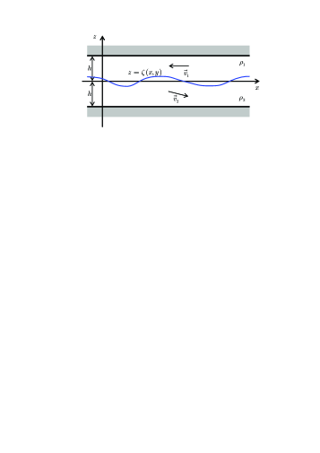
Figure 1: Sketch of a two-layer fluid system subject to harmonic horizontal vibrations and the coordinate frame.

2 Governing equations for large-scale patterns

With the standard multiscale method one can derive, that large-scale (or long-wavelength) patterns in the system of inviscid liquids are governed by the equation system [8]

$$\left\{\begin{array}[]{rcl}\displaystyle B_{0}\frac{\rho_{2}+\rho_{1}}{\rho_{\ast}}T^{2}\frac{\partial\varphi}{\partial t}\!\!\!&\displaystyle=&\!\!\!\displaystyle\left[L^{2}-\frac{h^{2}}{3}\right]\frac{\partial^{2}\eta}{\partial x^{2}}\\[15.0pt] &&\displaystyle{}+\frac{3}{2h}\frac{\rho_{2}-\rho_{1}}{\rho_{2}+\rho_{1}}\eta^{2}+\frac{B_{1}}{B_{0}}\eta\,,\\[15.0pt] \displaystyle\frac{\partial\eta}{\partial t}\!\!\!&\displaystyle=&\!\!\!\displaystyle-h\frac{\partial^{2}\varphi}{\partial x^{2}}\,.\end{array}\right.$$ (1)

Here $\eta(x,t)$ is the non-pulsating part of the interface displacement from the flat state, $\varphi(x,t)$ is the non-pulsating part of the upper fluid flow ($\vec{v}_{1}=-\nabla\varphi+...$, $\vec{v}_{2}=\nabla\varphi+...$, where “$...$” stands for the pulsing part of the flow and smaller corrections); notice $\varphi(x,t)$ is independent of $z$, since $\vec{v}_{1,2}$ are nearly constant along $z$. Reference length $L=\sqrt{\alpha/[(\rho_{2}-\rho_{1})g]}$, $\alpha$: surface tension, $\rho_{1}$ and $\rho_{2}$: density of the upper and lower fluids, respectively, $\rho_{1}<\rho_{2}$, $g$: gravity, $h$: unperturbed thickness of the layers, $T=L/b$: reference time, $\rho_{\ast}$: reference fluid density ($\rho_{\ast}$ can be chosen as convenient). Parameter $B$ is the dimensionless vibration parameter;

$$B\equiv\rho_{\ast}b^{2}/\sqrt{\alpha(\rho_{2}-\rho_{1})g}=B_{0}+B_{1}\,,$$ (2)

where $b$ is the container vibration velocity amplitude; $B_{0}$ is the linear instability threshold

$$B_{0}=\frac{\rho_{\ast}(\rho_{2}+\rho_{1})^{3}h}{2\rho_{1}\rho_{2}(\rho_{2}-\rho_{1})^{2}}\sqrt{\frac{(\rho_{2}-\rho_{1})g}{\alpha}}\,,$$ (3)

and $B_{1}$ is the deviation from the stability threshold.

We consider the system dynamics slightly below the linear instability threshold, i.e., for $B_{1}<0$ and $|B_{1}|\ll B_{0}$. With rescaling

$$\begin{array}[]{c}x\to x\,L\sqrt{\frac{B_{0}}{(-B_{1})}\left[1-\frac{h^{2}}{3L^{2}}\right]}\,,\quad\eta\to\eta\,h\frac{\rho_{2}+\rho_{1}}{\rho_{2}-\rho_{1}}\frac{(-B_{1})}{B_{0}}\,,\\[10.0pt] t\to t\sqrt{\frac{\rho_{2}-\rho_{1}}{\rho_{\ast}}\frac{L^{3}B_{0}^{3}}{h\,b^{2}B_{1}^{2}}\left[1-\frac{h^{2}}{3L^{2}}\right]}\,,\mbox{ and}\\[10.0pt] \varphi\to\varphi\sqrt{\frac{\rho_{\ast}(\rho_{2}+\rho_{1})^{2}}{(\rho_{2}-\rho_{1})^{3}}\frac{L^{3}B_{1}^{2}}{h\,b^{2}B_{0}^{3}}\left[1-\frac{h^{2}}{3L^{2}}\right]}\,,\end{array}$$ (4)

the governing equations (1) take zero-parametric dimensionless form;

$$\dot{\varphi} = \eta_{xx}+{\textstyle\frac{3}{2}}\eta^{2}-\eta\,,$$ (5)

$$\dot{\eta} = -\varphi_{xx}\,.$$ (6)

Here subscripts denote the partial derivative with respect to the specified coordinate.

The latter equation system can be recast as a ‘plus’ Boussinesq equation (BE);

$$\ddot{\eta}-\eta_{xx}+\left({\textstyle\frac{3}{2}}\eta^{2}+\eta_{xx}\right)_{xx}=0\,.$$ (7)

From the view point of dynamics, this equation essentially differs from original Boussinesq equation B (BE B) for waves in a shallow water layer [13] or in a two-layer system without vibrations [14], which is

$$\ddot{\eta}-\eta_{xx}-\left({\textstyle\frac{3}{2}}\eta^{2}+\eta_{xx}\right)_{xx}=0\,.$$ (8)

The equation system (5)–(6) is rigorously derived for the vicinity of the vibrational instability threshold (e.g., one cannot consider the case of vanishing vibrations, when departure from the threshold is finite, with this equation system). On the contrast, the Boussinesq equation A (BE A) [13] with nonlinear term $[(\varphi_{x})^{2}+(1/2)\eta^{2}]$ in place of $(3/2)\eta^{2}$ in Eq. (8) is derived for small dispersion and nonlinear terms, i.e., only small-amplitude waves with velocity close to $1$ are quantitatively governed by BE A. With assumptions required by BE A, one needs further to restrict consideration to the case of the wave package moving in one direction for to set $(\varphi_{x})^{2}=(\dot{\varphi})^{2}\approx\eta^{2}$ and obtain BE B (Eq. (8)). Summarizing, the results on soliton waves derived with BE B are rigorous for waves in shallow water only for the edge of the soliton spectrum and never rigorous for collisions of contrpropagating solitons, while Eq. (7) is rigorous for interfacial waves in the system subject to horizontal vibrations.

The integrability of the ‘plus’ BE was considered in [12] where the $\partial$-dressing method was employed for deriving multisoliton solutions. Bogdanov and Zakharov [12] reported existence of unstable solitons which can decay into pairs of stable solitons and thoroughly treated bounded states of two and more ‘singular’ solitons of the form $\eta=-4/(x-x_{0})^{2}$. For our system the ‘singular’ solitons cannot be considered as the long-wavelength approximation is violated for them. As Ref. [12] does not provide answers to some significant questions and omit certain important scenarios of the system dynamics, it will be more convenient to perform a comprehensive analysis of the system dynamics, without employment of a laborious $\partial$-dressing technique, and postpone comparison of this analysis to [12] for the Discussion section.

3 Solitons

Equation system (5)–(6) admits solutions in the form of propagating wave with time-independent profile; $\eta(x,t)=\eta(x-ct)\equiv\eta(\xi)$, $\varphi(x,t)=\varphi(x-ct)\equiv\varphi(\xi)$, where $c$ is the wave propagation speed. For these waves $\partial_{x}=\partial_{\xi}$ and $\partial_{t}=-c\partial_{\xi}$, and Eqs. (5)–(6) yield

$$\textstyle 0=\eta_{\xi\xi}+\frac{3}{2}\eta^{2}-(1-c^{2})\eta\,.$$ (9)

(Here we used the condition $\eta(\xi=\pm\infty)=0$.) The latter equation admits the soliton solution

$$\eta_{0}(\xi)=\frac{1-c^{2}}{\displaystyle\cosh^{2}\big{[}\sqrt{1-c^{2}}\xi/2\big{]}}\,;$$ (10)

for a given initial profile $\eta(x)$, the propagation direction ($+c$ or $-c$) is determined by the flow, $\varphi_{\xi}=\pm c\eta(\xi)$ (cf. Eq. (6)). The family of solitons is one-parametric, parameterized by the speed $c$ only. Speed $c$ varies within the range $[0,1]$; the standing soliton ($c=0$) is the sharpest and the highest one, while for the fastest solitons, $c\to 1$, the width tends to infinity ($\propto 1/\sqrt{1-c^{2}}$) and the height tends to $0$ ($\propto[1-c^{2}]$).

Let us interpret these results in original dimensional space–time. The spatial and temporal scales for dynamic system (5)–(6) depend on the deviation from the threshold $(-B_{1})$ (see rescaling (4)). For a transparent interpretation of the dynamics of patterns in original dimensional space–time, one can consider solitons for the dimensional equation system (1) and find equation of form (9) with coefficient

$$G:=\frac{(-B_{1})}{B_{0}}-c_{\mathrm{dim}}^{2}\frac{(\rho_{2}+\rho_{1})\,\alpha^{1/2}}{h\,[(\rho_{2}-\rho_{1})g]^{3/2}}$$ (11)

ahead of the last term $(-\eta)$, where $c_{\mathrm{dim}}$ is the dimensional speed of the soliton, with all the other coefficients being physical parameters of the physical system under consideration. Considering a given physical system with vibration parameter $B$ as a control parameter, one can see that the shape of a soliton is controlled by expression (11). Hence, the same interface inflection soliton can exist for different deviation $B_{1}$, but the same $G$, which will be achieved by tuning $c_{\mathrm{dim}}$; for larger negative deviation $(-B_{1})$ from the instability threshold, the speed $c_{\mathrm{dim}}$ is larger.

The family of solitons can be compared against the wave packages of linear waves—small perturbation of the flat-interface state. For small normal perturbations $(\eta,\varphi)\propto e^{i(kx-\Omega t)}$, Eqs. (5)–(6) yield the dispersion relation $\Omega(k)=k\sqrt{1+k^{2}}$. The group velocity is

$$v_{\mathrm{gr}}=\frac{d\Omega}{dk}=\frac{1+2k^{2}}{\sqrt{1+k^{2}}}\,,$$ (12)

which varies from $v_{\mathrm{gr}}=1$ (for $k\to 0$) to infinity (for $k\to\infty$). Thus, any packages of linear waves travel with higher velocity than the fastest solitons.

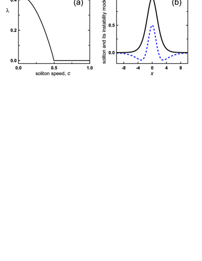
Figure 2: (a): Exponential growth rate $\lambda$ of perturbations of the soliton vs soliton speed $c$. (b): Soliton (black solid line) and its instability mode (blue dashed line) for $c=0$.

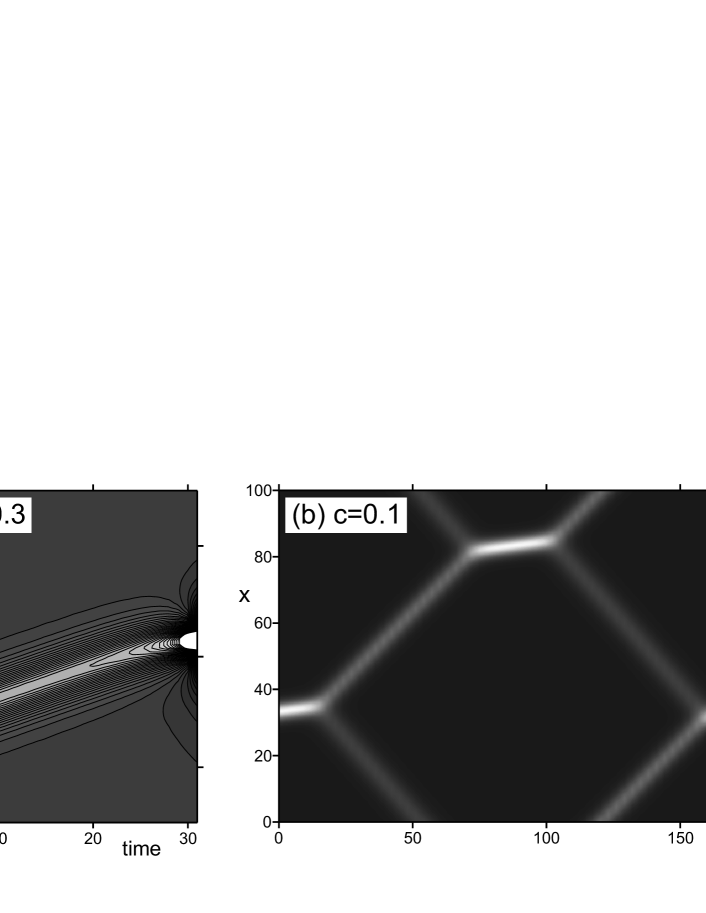
Figure 3: Two scenarios of nonlinear evolution of perturbations of unstable solitons. (a): Explosion of unstable soliton with $c=0.3$. (b): Falling-apart of unstable soliton with $c=0.1$ and recoalescence of the stable decay products.

4 Stability of solitons (initial perturbations)

The linear stability analysis for solitons in dynamic system (5)–(6) reveals that the slow solitons, with $0\leq c\leq 1/2$, are unstable (see Fig. 2(a)), with one unstable degree of freedom (in Fig. 2(b), one can see the instability mode for $c=0$). The fast solitons, with $1/2<c\leq 1$, are stable both linearly and to non-large finite perturbations. Detailed analysis of the linear stability can be found in [8].

It is interesting to consider the nonlinear development of perturbations of unstable solitons. Two possible scenarios were encountered in direct numerical simulations:
(i) Explosive growth of perturbation and formation of an infinitely sharp and high peak in a finite time;
(ii) Falling-apart of the unstable soliton into exactly two stable ones.
In Fig. 3, one can see the development of these scenarios.

Obviously, for the scenario (i), after violation of the conditions of the long-wavelength approximation, the dynamics will deviate from the one dictated by Eqs. (5)–(6); still, the formation of an sharpening of the interface with large deviation from the flat state is certain. In the following we will derive scaling laws for this explosion regime.

For the falling-apart of the unstable solution, we can observe in Fig. 3(b) that two fast solitons can then collide and coalesce again into the same initial unstable soliton, which will exist for awhile. The smaller perturbation of this unstable soliton, the longer it exists before falling apart again. It suggests that collisions of solitons can be ‘inelastic’. In the text below, we will investigate the collisions of fast stable solitons numerically and reveal analytical conditions for coalescence of colliding solitons, elastic collisions and explosions (notice, in Fig. 3(b) we observe collision not for an arbitrary pair of stable solitons but for the products of decay of the unstable soliton).

Noteworthy, one can predict wether the initial infinitesimal perturbation will lead to one or another scenario. It is determined by the projection of the initial perturbation onto the unstable mode. According to results of direct numerical simulation, if one normalizes the instability mode $(e^{\lambda t}\eta_{1}(\xi),e^{\lambda t}\varphi_{1}(\xi))$ so that $\eta_{1}(0)>0$—cf. Fig. 2(b), where the instability mode for the soliton with $c=0$ is plotted with the blue dashed line—then the perturbation with a positive contribution of $(\eta_{1}(\xi),\varphi_{1}(\xi))$ will lead to explosion while the one with a negative contribution will lead to the splitting.[]

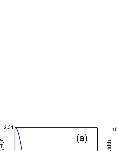
Figure 4: (a): Profiles of the explosively growing spike from Fig. 3(a) for $(t_{\ast}-t)=0.1$, $0.2$, $0.3$, $0.4$, $0.5$, $0.6$ (where $t_{\ast}$ is the time instant when $\eta_{\mathrm{max}}\to\infty$) are nearly indistinguishable after rescaling. (b): The behavior of the spike width (blue squares) and height (red circles) is compared to the scaling laws $6.448\sqrt{t_{\ast}-t}$ and $2.309/(t_{\ast}-t)$, respectively, dictated by Eq. (14) with $n=-1$, $m=1/2$ for $\eta\gg 1$.

5 Explosions

For the explosion solution, field $\eta$ becomes large and the term $(-\eta)$ can be neglected against the background of the term $(3/2)\eta^{2}$ in Eq. (5); therefore, equation system (5)–(6) can be rewritten as

$$\ddot{\eta}\approx-\big{(}\eta_{xx}+{\textstyle\frac{3}{2}}\eta^{2}\big{)}_{xx}\,.$$ (13)

The last differential equation is homogeneous: it admits self-similar solutions of the form

$$\eta(x,t)=t^{n}f(s),\qquad s=x/t^{m}\,,$$ (14)

where $n$ and $m$ are to be determined from the condition that Eq. (13) yields a differential equation for $f(s)$ which is free from $t$ and $x$. After substitution (14), Eq. (13) reads

$$\begin{array}[]{r}n(n-1)f-m(2n-m-1)sf^{\prime}+m^{2}s^{2}f^{\prime\prime}\\[10.0pt] =-t^{2-4m}\big{[}f^{\prime\prime}+\frac{3}{2}t^{n+2m}f^{2}\big{]}^{\prime\prime}\,,\end{array}$$

i.e. requires $m=1/2$ and $n=-1$. With these values of $n$ and $m$ the equation for $f(s)$ reads

$$\textstyle f^{\prime\prime\prime\prime}+\frac{3}{2}(f^{2})^{\prime\prime}+\frac{1}{4}s^{2}f^{\prime\prime}+\frac{7}{4}sf^{\prime}+2f=0\,.$$ (15)

The last equation has unique solution neither diverging at $s=0$ nor nonvanishing at $s\to\pm\infty$. This solution is

$$f(s)=8\big{(}3\sqrt{2}-s^{2}\big{)}/\big{(}3\sqrt{2}+s^{2}\big{)}^{2}\,.$$ (16)

In Fig. 4(a), one can see that the rescaled profiles of the explosion solution from Fig. 3(a) become nearly indistinguishable from the solution $f(s)$ to Eq. (15) quite quickly.

While the solitons are running, the explosive solution is standing. This can be seen as well in Fig. 3(a), where the pattern stops when the explosion happens.

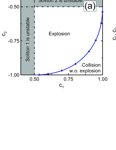
Figure 5: (a): Collision map for contrpropagating solitons. On the blue curve, colliding solitons coalesce; on the one side of the curve, collisions result in explosion, while on the other side, collisions are elastic. The results of direct numerical simulation are plotted with triangles; the blue curve represents the solution to algebraic system (21)–(22) for soliton coalescence. (b): Speeds of coalescing solitons $c_{1}$ and $c_{2}$ on the collision instability boundary are plotted versus $c_{0}$, the unstable soliton speed forming as a result of coalescence. The black curves correspond to collision of contrpropagating solitons. The blue dash-dotted curve corresponds to the formal coalescence solution for copropagating solitons, which is not observed in direct numerical simulation; copropagating solitons exchange their momentum from distance, without formation of a single peak interface profile at any stage of the collision event.

6 Integrals of motion

As an integrable system, BE possesses infinite number of integrals of motion. In particular, one can show the dynamic system (5)–(6) to possess two following independent integrals of motion[]:

$$I_{0} \textstyle=\int_{-\infty}^{+\infty}\eta(x,t)\,\mathrm{d}x\,,$$ (17)

$$I_{1} \textstyle=\int_{-\infty}^{+\infty}\eta(x,t)\,\varphi_{x}(x,t)\,\mathrm{d}x\,.$$ (18)

The first integral is owned by the mass conservation law and the second integral represents the momentum conservation law—thus, the both conservation laws valid for the virgin fluid dynamical system have their reflections in presented integrals of motion of the system (5)–(6). These integrals will be useful for our following consideration.

For the soliton (10), one can find

$$I_{0}[\eta_{0}(x-ct)] \textstyle=\int_{-\infty}^{+\infty}\eta_{0}\,\mathrm{d}x=\sqrt{1-c^{2}}\,,$$ (19)

$$I_{1}[\eta_{0}(x-ct)] \textstyle=c\int_{-\infty}^{+\infty}\eta_{0}^{2}\,\mathrm{d}x=c\left[1-c^{2}\right]^{3/2}.$$ (20)

Here it is important, that soliton velocity $c$ in Eq. (20) is negative for solitons propagating to the left.

7 Two-soliton collisions

While the system dynamics is integrable, the possibility of explosions and the coalescence of decay products of an unstable soliton (as seen in Fig. 3(b)) suggest that collision of stable solitons can be ‘inelastic’. The results of direct numerical simulation of the collisions of pairs of solitons are presented in Fig. 5(a). Collisions of copropagating solitons are always elastic and they exchange their velocities during this collisions. Collisions of contrpropagating solitons can be either elastic, when solitons are fast enough, or lead to an explosion. With elastic collision, they exchange velocities and effectively transpass through one another. At the explosion boundary, solitons are found to coalesce, forming an unstable soliton. It is interesting to consider this coalescence and the decay of unstable solitons into two stable products from the perspective of the motion integrals. Indeed, for solitons that are at the distance from each other the profiles are nearly mutually unaffected and $I_{j}=I_{j}[\eta_{0}(x-c_{1}t,c_{1})]+I_{j}[\eta_{0}(x-c_{2}t,c_{2})]$, where $c_{2}<0$, which should be the same as for the coalescence product soliton of velocity $c_{0}$. These integrals are best to be recast in terms of $Z_{j}\equiv\sqrt{1-c_{j}^{2}}$;

$$Z_{1}+Z_{2} =Z_{0}\,,$$ (21)

$$Z_{1}^{3}\sqrt{1-Z_{1}^{2}}-Z_{2}^{3}\sqrt{1-Z_{2}^{2}} =Z_{0}^{3}\sqrt{1-Z_{0}^{2}}\,.$$ (22)

For any $Z_{0}\in(1/\sqrt{2};1]$, which corresponds to $c_{0}\in[0;1/2)$, i.e. an unstable soliton, a pair of solutions $Z_{1}$ and $Z_{2}$ exist, both of which are in the semi-open interval $(0;1/\sqrt{2}]$, i.e. correspond to stable solitons with $|c_{j}|\in[1/2;1]$. For $Z_{0}<1/\sqrt{2}$ the equation system (21)–(22) has no solution. Thus, one obtains the soliton collision instability boundary semi-analytically, with the solution to algebraic equation system (21)–(22). This solution is plotted in Fig. 5(a) with the solid blue line and one can see this result to match the results of direct numerical simulation plotted with triangles. In Fig. 5(b) one can see relations between $c_{0}$ and the pair $c_{1}$ and $|c_{2}|<c_{1}$.

This result is quite interesting: half of solitons, with $c\in[0,1/2)$, are unstable and can be represented as a superposition of two solitons from the other half of them, with $c\in[1/2,1)$. The solitons of the latter half are stable and cannot be decomposed into other solitons. Moreover, the unstable solitons are not merely the superposition of stable ones, they are also the boundary of the basin of the system trajectories leading to an explosive rapture of the upper layer.

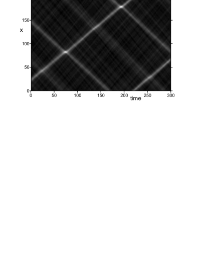
Figure 6: Sample evolution of the dynamic system (5)–(6) with arbitrary initial conditions: the dynamics turns out to be a kinetics of a gas of stable (fast) solitons experiencing collisions.

8 Discussion

In Fig. 6, a sample of the system dynamics from arbitrary initial conditions is presented in domain $x\in[0;200]$ with periodic boundary conditions. One can see this dynamics can be well treated as a kinetics of a gas of stable solitons.

Let us compare the big picture of the system dynamics constructed above with the results from [12] where the dynamics of the ‘plus’ Boussinesq equation was considered on manifolds of superpositions of finite number of solitons. Two subfamilies of stable and unstable solitons were revealed in [12] as well, however their stability was not considered with respect to arbitrary perturbations. While the decay of an unstable soliton into pair of stable solitons was reported with explicit analytical solutions, possibility of an ‘explosion’ of single unstable soliton was not reported. Thus, the picture of scenarios of instability development was incomplete. Although the formation of an explosion can be seen in [12] for collisions of two unperturbed unstable solitons, its universal asymptotic shape (Eq. (16)) and scaling properties (Eq. (14)) were not considered. For the problem of two-soliton collisions, there were two general conclusions in [12]: (1) stable copropagating solitons “do not form singularities as a result of two-soliton interaction” (which is important for us, as we observe no explosions and no coalescences for copropagating solitons) and (2) two-soliton interaction of unstable solitons necessarily leads to formation of a singularity. In the light of the results of the analysis of stability with respect to arbitrary perturbations, the latter statement becomes less informative. The case of collision of contrpropagating stable solitons, which yields us most important results, was not addressed previously. Ref. [12] stands as a prominent work in the theory of solitons, presenting general multi-soliton solution for a paradigmatic ‘plus’ Boussinesq equation, the phenomenon of decay of unstable solitons into pairs of stable ones, and forth and back transformations of interacting solitons into bounded states of singularities.

9 Conclusion

We presented a comprehensive analysis of the dynamics resulting from the nonlinear evolution equations for long-wavelength patterns in a system of two layers of immiscible inviscid fluids subject to horizontal vibrations. In this system the standing and slow solitons, $c<1/2$, are unstable, while the fast solitons, $c\geq 1/2$, are stable. For unstable solitons, nonlinear stages of development of perturbations lead to either an ‘explosion’ or to falling-apart of an unstable soliton into pair of stable solitons. The self-similar explosion soliton was derived and found to agree well with the results of direct numerical simulation. Two integrals of motion were obtained and employed for demonstrating that unstable solitons can be represented by superpositions of pairs of stable ones, while stable solitons are elementary. We found that soliton collisions can be either elastic or lead to an explosion; at the boundary between elastic and explosive collisions, colliding stable solitons coalesce into unstable ones. To conclude, beyond the vicinities of explosions, the system dynamics is completely representable by a kinetics of a soliton gas and the system is fully integrable. Coexistence of explosion solutions and integrability for a real physical system is quite remarkable.

- [1] \NameWolf G. H. \REVIEWZ. Phys.2271961291.
- [2] \NameWolf G. H. \REVIEWPhys. Rev. Lett.241970444.
- [3] \NameLyubimov D. V. Cherepanov A. A. \REVIEWFluid Dynamics211987849.
- [4] \NameKhenner M. V., Lyubimov D. V. Shotz M. M. \REVIEWFluid Dynamics331998318.
- [5] \NameKhenner M. V., Lyubimov D. V., Belozerova T. S. Roux B. \REVIEWEuropean Journal of Mechanics B/Fluids1819991085.
- [6] \NameShklyaev S., Alabuzhev A. A. Khenner M. \REVIEWPhys. Rev. E792009051603.
- [7] \NameBenilov E. S. Chugunova M. \REVIEWPhys. Rev. E812010036302.
- [8] \NameGoldobin D. S., Kovalevskaya K. V., Lyubimov D. V.Lyubimova T. P. \REVIEWunpublished, E-print arxiv:1406.77042014.
- [9] \NameZamaraev A. V., Lyubimov D. V. Cherepanov A. A. \REVIEWHydrodynamics and Processes of Heat and Mass Transfer (Sverdlovsk: Ural Branch of Acad. of Science of USSR)198923 [in Russian]. (The results of this work related to the problem we consider also follow from [3])
- [10] \NameOrlov A. Yu. \BookCollapse of solitons in integrable models, Preprint IAiE No. 221 \PublIAiE, Novosibirsk \Year1983.
- [11] \NameFalkovich G. E., Spector M. D. Turitsyn S. K. \REVIEWPhys. Lett. A991983271.
- [12] \NameBogdanov L. V. Zakharov V. E. \REVIEWPhysica D1652002137.
- [13] \NameBoussinesq J. \REVIEWJournal de Mathématiques Pures et Appliquées17187255.
- [14] \NameChoi W. Camassa R. \REVIEWJ. Fluid Mech.39619991.