The SU(3) Algebra in a Cyclic Basis

Abstract

With the couplings between the eight gluons constrained by the structure constants of the su(3) algebra in QCD, one would expect that there should exist a special basis (or set of bases) for the algebra wherein, unlike in a Cartan-Weyl basis, all gluons interact identically (cyclically) with each other, explicitly on an equal footing. We report here particular such bases, which we have found in a computer search, and we indicate associated $3\times 3$ representations. We conjecture that essentially all cyclic bases for su(3) may be obtained from these making appropriate circulant transformations, and that cyclic bases may also exist for other su($n$), $n>3$.

1. Introduction: Both the su(2) and su(3) algebras Note (1) are central to contemporary particle-physics theory, as the two non-Abelian real Lie algebras generating the unitary weak-isospin and colour symmetry groups underlying the Standard Model of (purely-) weak and strong forces respectively. The relevant gauge bosons in each case appear in the adjoint representation of the algebra, with the self-couplings among the three weak bosons and among the eight gluons thereby constrained by the structure constants of the algebra, ensuring gauge invariance.

Regarding the weak sector for example []WEIN; *GLASH; *SALAM the su(2) algebra may be readily expressed by considering basis elements $\hat{w}_{i}$ satisying the su(2) algebra in the form:

$$[\hat{w}_{1},\hat{w}_{2}]=\hat{w}_{3}\hskip 14.22636pt[\hat{w}_{2},\hat{w}_{3}]=\hat{w}_{1}\hskip 14.22636pt[\hat{w}_{3},\hat{w}_{1}]=\hat{w}_{2},\hskip 14.22636pt$$ (1)

familiar as the ordinary 3-space vector-product rule, or also as the commutation relations of the normalised Pauli matrices ($\hat{w}_{i}\leftrightarrow-i\sigma_{i}/2$, where ${\rm Tr}\,\sigma_{i}.\sigma_{j}=2\delta_{ij}$). The three corresponding weak-isospin gauge-field components, $W_{1}$, $W_{2}$, $W_{3}$, may then be incorporated in the Lagrangian (at least as concerns the pure-gauge part, see e.g. Ref. []ATIY; *SMIT) as coefficients of the corresponding $3\times 3$ adjoint representation matrices, as determined by the structure constants implicit in Eq. 1. The above circulant or cyclic form (Eq. 1) for su(2) has the reassuring feature that clearly all three weak field components will appear on an explicitly equal footing, with no weak-isospin direction distinguished.

On the other hand, the algebra Eq. 1, when viewed as a complex Lie algebra (namely $A_{1}$) expressed in the Chevalley basis, takes the canonical (non-cyclic) form:

$$[\hat{w}^{\prime}_{3},\hat{w}^{\prime}_{1}]=2\hat{w}^{\prime}_{1}\hskip 42.67912pt[\hat{w}^{\prime}_{3},\hat{w}^{\prime}_{2}]=-2\hat{w}^{\prime}_{2}$$

$$[\hat{w}^{\prime}_{1},\hat{w}^{\prime}_{2}]=\hat{w}^{\prime}_{3}\hskip 65.44142pt$$ (2)

which, in the present context, might be seen as better aligned with the physical states after spontaneous symmetry breaking. In the Standard Model, it is the non-zero Higgs field which picks-out a particular direction in weak-isospin space to define the 3rd weak-isospin component, which then mixes with the U(1) hypercharge boson to form the photon and the $Z$-boson, with the two transverse components combined (as the $\pm 1$ eigenstates of $I_{3}$) to describe the charged weak bosons, $W^{+}$ and $W^{-}$. The two forms Eq. 1 and Eq. 2 (of the complex algebra A₁) are related by the (complex) transformation:

$$\left(\begin{matrix}\hat{w}^{\prime}_{1}\cr\hat{w}^{\prime}_{2}\cr\hat{w}^{\prime}_{3}\end{matrix}\right)\!\!=\!\!\left(\begin{matrix}i\>&\>-1&\cr i\>&\>+1&\cr&&\>2i\end{matrix}\right)\!\!\left(\begin{matrix}\hat{w}_{1}\cr\hat{w}_{2}\cr\hat{w}_{3}\end{matrix}\right).\!\!$$ (3)

While Eq. 2 may be viewed as an expression of the (real but non-compact) Lie algebra sl(2,R) $\simeq$ su(1,1), the corresponding representation matrices can still be utilised in constructing the Lagrangian, provided that they are coupled with the appropriately defined (complex) field components (proportional to $W^{+}=(W_{1}-iW_{2})/\sqrt{2}$, $W^{-}=(W_{1}+iW_{2})/\sqrt{2}$ and $W_{3}$) such that the action remains unchanged. Naturally, the theory remains SU(2) gauge invariant, and all physical consequences, before or after spontaneous symmetry breaking, remain undisturbed by such a change of basis.

In the case of the strong interaction (QCD) the SU(3) colour symmetry is well-known to be unbroken, and we may expect that the theoretical prediction of any measurable will always result as summed or averaged symmetrically over colours and hence be readily expressible in an explicitly basis-independent way. Somewhat analogous to the Pauli matrices for su(2), in the case of su(3) one has the Gell-Mann matrices, $\lambda_{a}$ []GELL; *NEEM, $a=1\dots 8$ (with ${\rm Tr}\,\lambda_{a}.\lambda_{b}=2\delta_{ab}$, $a,b=1\dots 8$), which constitute a $3\times 3$ matrix representation of the su(3) algebra in the form ($\hat{g}_{a}\leftrightarrow-i\lambda_{a}/2$):

$$[\hat{g}_{1},\hat{g}_{2}]=\hat{g}_{3}\hskip 22.76219pt[\hat{g}_{1},\hat{g}_{4}]=\hat{g}_{7}/2\hskip 22.76219pt[\hat{g}_{1},\hat{g}_{5}]=-\hat{g}_{6}/2\hskip 25.60747pt$$

$$\hskip 2.84526pt[\hat{g}_{2},\hat{g}_{4}]=\hat{g}_{6}/2\hskip 8.53581pt[\hat{g}_{2},\hat{g}_{5}]=\hat{g}_{7}/2\hskip 8.53581pt[\hat{g}_{4},\hat{g}_{5}]=\hat{g}_{3}/2+\sqrt{3}/2\hat{g}_{8}\hskip 8.53581pt$$

$$\hskip 2.84526pt[\hat{g}_{4},\hat{g}_{8}]=-\sqrt{3}/2\hat{g}_{5}\hskip 25.60747pt[\hat{g}_{6},\hat{g}_{7}]=-\hat{g}_{3}/2+\sqrt{3}/2\hat{g}_{8}\hskip 31.29802pt$$ (4)

where the Lie brackets quoted (Eq. 4) are sufficient to determine all non-zero brackets, given that the su(3) structure constants are totally antisymmetric in the Gell-Mann basis. One sees almost immediately however that the su(3) algebra in the form specified by Eq. 4 is far from cyclic (cf. Eq. 1), whereby the Pauli basis for su(2) and Gell-Mann basis for su(3) cannot be considered fully analogous, at least in this respect.

Choice of basis for the algebra being of conceptual importance here, we find ourselves motivated to ask if a cyclic basis, with all eight gluons in the same relative relationship, analogous to Eq. 1 for su(2), actually exists (or not) for the case of su(3). Our best literature search uncovered just one allusion Rossi (1973) to a “cyclic basis” (Eq. 1) for su(2), but no mention of any such equivalent for su(3), or indeed for any su($n$), $n>2$ (or for any other Lie algebra). Having thus had to rely on our own efforts in attempting to answser this question, we are now able to report what we believe to be the complete set of such cyclic bases for su(3) (and for a few other very closely related Lie algebras). In the following sections we briefly outline our methods and proceed to document the cyclic forms we obtained. As a by-product, we are able to give a set of $3\times 3$ matrices which constitute a matrix representation of the su(3) algebra in cyclic form, very closely analogous to the Pauli matrices for su(2). These matrices (at least as regards their general form/symmetries etc.) in fact turn out to be familiar to us already in a somewhat different particle-physics context Harrison and Scott (1994); *SCOTT, as will be detailed later (see Section 4).

2. A ‘Theorem’ and a Computer Search: In a heuristic spirit, let us suppose that such cyclic forms exist for at least some Lie algebras beyond su(2). In particular, taking su(3) as an example, we would then expect (in analogy to Eq. 1 for the su(2) case) to be able to write all brackets in the form:

$$[\hat{g}_{a},\hat{g}_{b}] = f_{ab}^{c}\,\hat{g}_{c}\hskip 11.38092pt{\rm with}\hskip 8.5359ptf_{a+x\,b+x}^{c+x}=f_{ab}^{c},\hskip 11.38092pt$$

$${\rm where}\hskip 2.84544pt x=1\dots 8\hskip 22.76228pt{\rm indices}\hskip 5.69046pt{\rm mod}\hskip 5.69046pt8,1\hskip 22.76228pt$$ (5)

and where “indices mod 8,1” implies a cyclic interpretation of subscripts and superscipts, such that $7+1=8$, $8+1=1$ etc. The algebra being expressed in this form, with all basis elements, $\hat{g}_{1}\dots\hat{g}_{8}$, appearing cyclically on an explicitly equal footing, precisely generalises the su(2) case (Eq. 1). We add that it will prove useful to visualise the base elements in such a basis

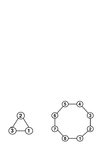
Figure 1: In a cyclic basis, the base elements of su(2) and su(3) are usefully visualised as being located at the vertices of an equilateral triangle and regular octagon respectively.

as being located at the vertices of a regular polygon, i.e. at the corners of an equilateral triangle in the su(2) case, or at the corners of a regular octagon in the case of su(3), as illustrated (for subsequent reference) in Figure 1.

Now, given a real Lie algebra such as su(3), we can always transform to a new basis with any real non-singular linear transformation we choose. Along with the transformation of the basis elements, $\hat{g}_{a}$, the structure constants, $f_{ab}^{c}$, will transform, in a tensor-like fashion, with two covariant and one contravariant index. Applying such a transformation (with transformation matrix $C$) to the cyclic form, Eq. 5, above:

$$(\hat{g}_{a}^{\prime})^{T}\,\,=\,\,C\,.\,(\hat{g}_{a})^{T}$$ (6)

where $(\hat{g}_{a})=(\hat{g}_{1},\dots,\hat{g}_{8})$ and $(\hat{g}_{a}^{\prime})=(\hat{g}_{1}^{\prime},\dots,\hat{g}_{8}^{\prime})$, we take it as self-evident that, if the transformation takes the form of a (+1)-circulant matrix Davis (1979):

$$C={\rm circ}(c_{1},c_{2},c_{3},c_{4},c_{5},c_{6},c_{7},c_{8})$$ (7)

that is, if:

$$\left(\begin{matrix}\hat{g}_{1}^{\prime}\cr\hat{g}_{2}^{\prime}\cr\hat{g}_{3}^{\prime}\cr\hat{g}_{4}^{\prime}\cr\hat{g}_{5}^{\prime}\cr\hat{g}_{6}^{\prime}\cr\hat{g}_{7}^{\prime}\cr\hat{g}_{8}^{\prime}\end{matrix}\right)=\left(\begin{matrix}c_{1}&c_{2}&c_{3}&c_{4}&c_{5}&c_{6}&c_{7}&c_{8}\cr c_{8}&c_{1}&c_{2}&c_{3}&c_{4}&c_{5}&c_{6}&c_{7}\cr c_{7}&c_{8}&c_{1}&c_{2}&c_{3}&c_{4}&c_{5}&c_{6}\cr c_{6}&c_{7}&c_{8}&c_{1}&c_{2}&c_{3}&c_{4}&c_{5}\cr c_{5}&c_{6}&c_{7}&c_{8}&c_{1}&c_{2}&c_{3}&c_{4}\cr c_{4}&c_{5}&c_{6}&c_{7}&c_{8}&c_{1}&c_{2}&c_{3}\cr c_{3}&c_{4}&c_{5}&c_{6}&c_{7}&c_{8}&c_{1}&c_{2}\cr c_{2}&c_{3}&c_{4}&c_{5}&c_{6}&c_{7}&c_{8}&c_{1}\cr\end{matrix}\right)\left(\begin{matrix}\hat{g}_{1}\cr\hat{g}_{2}\cr\hat{g}_{3}\cr\hat{g}_{4}\cr\hat{g}_{5}\cr\hat{g}_{6}\cr\hat{g}_{7}\cr\hat{g}_{8}\end{matrix}\right),$$ (8)

then the transformed algebra (basis $\hat{g}_{a}^{\prime}$) will also be cyclic. This ‘theorem’ clearly generalises to complex transformations, except of course that complex transformations may result in a different real form of the same (complex) algebra. This suggests that if we were just able to discover one cyclic form for su(3), we could immediately generate essentially all possible cyclic forms (for su(3) itself - or indeed for its complex extension A₂ and hence also for the sl(3,R) or su(2,1) real forms) by making appropriate (real or complex) circulant transformations.

At this point therefore, we resorted to a computer-based search aimed at finding at least one cyclic expression for the su(3) algebra. In a cyclic basis, in the 8-dimensional case (Figure 1 right), the four brackets:

$$[\hat{g}_{1},\hat{g}_{2}] = f_{12}^{1}\,g_{1}+f_{12}^{2}\,g_{2}+f_{12}^{3}\,g_{3}+f_{12}^{4}\,g_{4}$$ (9)

$$+f_{12}^{5}\,g_{5}+f_{12}^{6}\,g_{6}+f_{12}^{7}\,g_{7}+f_{12}^{8}\,g_{8}\hskip 17.07182pt$$

$$[\hat{g}_{1},\hat{g}_{3}] = f_{13}^{1}\,g_{1}+f_{13}^{2}\,g_{2}+f_{13}^{3}\,g_{3}+f_{13}^{4}\,g_{4}$$ (10)

$$+f_{13}^{5}\,g_{5}+f_{13}^{6}\,g_{6}+f_{13}^{7}\,g_{7}+f_{13}^{8}\,g_{8}\hskip 17.07182pt$$

$$[\hat{g}_{1},\hat{g}_{4}] = f_{14}^{1}\,g_{1}+f_{14}^{2}\,g_{2}+f_{14}^{3}\,g_{3}+f_{14}^{4}\,g_{4}$$ (11)

$$+f_{14}^{5}\,g_{5}+f_{14}^{6}\,g_{6}+f_{14}^{7}\,g_{7}+f_{14}^{8}\,g_{8}\hskip 17.07182pt$$

$$[\hat{g}_{1},\hat{g}_{5}] = f_{15}^{1}\,g_{1}+f_{15}^{2}\,g_{2}+f_{15}^{3}\,g_{3}+f_{15}^{4}\,g_{4}$$ (12)

$$+f_{15}^{5}\,g_{5}+f_{15}^{6}\,g_{6}+f_{15}^{7}\,g_{7}+f_{15}^{8}\,g_{8},\hskip 14.22636pt$$

together with the cyclic constraint (Eq. 5) and the Lie antisymmetry condition, are clearly sufficient to readily determine all brackets. Indeed, taking the cyclic constraint and the Lie antisymmetry condition together, Eq. 12 is readily re-cast to involve just four parameters as follows:

$$[\hat{g}_{1},\hat{g}_{5}] = f_{15}^{1}\,g_{1}+f_{15}^{2}\,g_{2}+f_{15}^{3}\,g_{3}+f_{15}^{4}\,g_{4}$$ (13)

$$-f_{15}^{1}\,g_{5}-f_{15}^{2}\,g_{6}-f_{15}^{3}\,g_{7}-f_{15}^{4}\,g_{8}.\hskip 17.07182pt$$

For a manageable computer search, in place of Eq. 13 (and thereby risking to miss valid instances), we in fact implemented the simpler condition:

$$[\hat{g}_{1},\hat{g}_{5}] = 0.\hskip 11.38092pt$$ (14)

Even so, we still had 24 structure constants $f_{12}^{c}$, $f_{13}^{c}$, $f_{14}^{c}$, $c=1\dots 8$ (Eqs. 9-11) to find, and our search was therefore restricted to trying only the values $+1$, $-1$ and $0$ for each of these 24 parameters. After $\sim\!\!100$ hours running on the RAL PPD linux farm Kelsey (2012), we found that, out of $3^{24}\simeq 2.8\times 10^{11}$ possibilities, a total of 972 choices fully satisfied the Jacobi relation (excluding cases where any of $f_{12}^{c}$, $f_{13}^{c}$, $f_{14}^{c}$=0, $\forall c=1\dots 8$). Then, in a second pass, selecting only cases with negative-definite Killing form (corresponding to the real algebra su(3) itself), just two cases remained as displayed in Table 1,

Case	$f_{12}^{c}$	$f_{13}^{c}$	$f_{14}^{c}$	metric
No.	$1\,2\,3\,4\,5\,6\,7\,8$	$1\,2\,3\,4\,5\,6\,7\,8$	$1\,2\,3\,45\,6\,7\,8$	signature
1	$0\,0\,1\,1\,0\,0\,\bar{1}\,1$	$0\,\bar{1}\,0\,\bar{1}\,0\,\bar{1}\,0\,1$	$0\,\bar{1}\,1\,0\,0\,\bar{1}\,\bar{1}\,0$	$(-24)^{8}$
2	$0\,0\,0\,1\,0\,0\,\bar{1}\,1$	$0\,\bar{1}\,0\,\bar{1}\,0\,\bar{1}\,0\,0$	$0\,\bar{1}\,1\,0\,0\,\bar{1}\,0\,0$	$(-18)^{4}$, $(-6)^{4}$

Table 1: The two sets of cyclic structure constants for the Lie algebra su(3) found in our computer search (only structure-constant values of $+1$, $0$, $-1$ were tried, as indicated here by $1$, $0$, $\bar{1}$ respectively). The last column gives the eigenvalues of the Killing metric with their multiplicities.

excluding cases trivially related to these by overall sign change, or/and by simple reversal of the cyclic ordering - see below.

3. Transformations between Cyclic Forms: Directly from Table 1: case 1   then, we have that the su(3) algebra may be expressed in the cyclic form:

$$\left[\hat{g}^{(1)}_{a+1},\hat{g}^{(1)}_{a+2}\right] = \hskip 7.11317pt\hat{g}^{(1)}_{a+3}+\hat{g}^{(1)}_{a+4}-\hat{g}^{(1)}_{a+7}+\hat{g}^{(1)}_{a+8}$$ (15)

$$\left[\hat{g}^{(1)}_{a+1},\hat{g}^{(1)}_{a+3}\right] = -\hat{g}^{(1)}_{a+2}-\hat{g}^{(1)}_{a+4}-\hat{g}^{(1)}_{a+6}+\hat{g}^{(1)}_{a+8}$$ (16)

$$\left[\hat{g}^{(1)}_{a+1},\hat{g}^{(1)}_{a+4}\right] = -\hat{g}^{(1)}_{a+2}+\hat{g}^{(1)}_{a+3}-\hat{g}^{(1)}_{a+6}-\hat{g}^{(1)}_{a+7}$$ (17)

$$\left[\hat{g}^{(1)}_{a+1},\hat{g}^{(1)}_{a+5}\right] = 0,\hskip 11.38092pt\hskip 8.5359pta=1\dots 8\hskip 14.22636pt{\rm mod}\;8,1.\hskip 28.45274pt$$ (18)

The Killing form is diagonal in this basis ($\kappa^{(1)}_{ab}=-24\delta_{ab}$) and the structure constants are totally antisymmetric. As regards economy of expression, it turns out that all structure constants Eqs. 15-18 could if necessary be readily inferred from Eq. 16 alone, exploiting the total antisymmetry and the cyclic property (Eq. 5) together.

From Table 1: case 2, we have that the real algebra su(3) may also be expressed:

$$\left[\hat{g}^{(2)}_{a+1},\hat{g}^{(2)}_{a+2}\right] = \hskip 7.11317pt\hat{g}^{(2)}_{a+4}-\hat{g}^{(2)}_{a+7}+\hat{g}^{(2)}_{a+8}$$ (19)

$$\left[\hat{g}^{(2)}_{a+1},\hat{g}^{(2)}_{a+3}\right] = -\hat{g}^{(2)}_{a+2}-\hat{g}^{(2)}_{a+4}-\hat{g}^{(2)}_{a+6}$$ (20)

$$\left[\hat{g}^{(2)}_{a+1},\hat{g}^{(2)}_{a+4}\right] = -\hat{g}^{(2)}_{a+2}+\hat{g}^{(2)}_{a+3}-\hat{g}^{(2)}_{a+6}$$ (21)

$$\left[\hat{g}^{(2)}_{a+1},\hat{g}^{(2)}_{a+5}\right] = 0,\hskip 11.38092pt\hskip 8.5359pta=1-8\hskip 14.22636pt{\rm mod}\;8,1.\hskip 28.45274pt$$ (22)

In this case the Killing form is circulant but not diagonal:

$$\kappa^{(2)}={\rm circ}\{-12,0,0,0,6,0,0,0\}.$$ (23)

The transformation from su(3) (Eqs. 15-18) to su(3) (Eqs. 19-22) is given by:

$$C^{(21)}={\rm circ}\{(1+\sqrt{3})/4,0,0,0,(1-\sqrt{3})/4,0,0,0\}$$ (24)

and the corresponding inverse transformation by:

$$C^{(12)}={\rm circ}\{(1+1/\sqrt{3}),0,0,0,(1-1/\sqrt{3}),0,0,0\}.$$ (25)

Cyclic forms satisfying Eq. 5 but related to case 1 and case 2 by trivial reversal of cyclic ordering and so excluded from Table 1, may then be generated by a (-1)-circulant (or retro-circulant Davis (1979)) transformation:

$$C^{(\bar{i}i)}=(-1){\rm circ}\{(0,0,0,0,0,0,0,1\}$$ (26)

having non-zero (unit) entries only on the trailing diagional. Our claim to have found the complete set of cyclic bases for su(3) and hence for the complex algebra $A_{2}$ and any of its real forms, rests on the plausible conjecture that any such basis may be reached with a combination of the transformation Eq. 26 and general circulant transformations Eqs. 6-8, with arbirary complex parameters.

4. Relation to the Gell-Mann Basis and the Gell-Mann Matrices: The Gell-Mann basis of su(3) is defined by Eq. 4. If we define:

$$x_{-}=1/\sqrt{3}-1\hskip 11.38092ptx_{0}=-2/\sqrt{3}\hskip 11.38092ptx_{+}=1/\sqrt{3}+1,$$ (27)

then the (real) transformation from cyclic su(3) (taking as an example the particular cyclic form Eqs. 15-18) to the Gell-Mann basis (Eq. 4) is given by:

$$\left(\begin{matrix}0&-\frac{x_{+}}{8}&\frac{x_{-}}{8}&-\frac{x_{0}}{8}&0&-\frac{x_{-}}{8}&\frac{x_{+}}{8}&-\frac{x_{0}}{8}\cr 0&\frac{x_{-}}{8}&-\frac{x_{+}}{8}&-\frac{x_{0}}{8}&0&-\frac{x_{+}}{8}&\frac{x_{-}}{8}&\frac{x_{0}}{8}\cr-\frac{\sqrt{3}\,x_{-}}{8}&0&0&0&\frac{\sqrt{3}\,x_{+}}{8}&0&0&0\cr 0&-\frac{x_{0}}{8}&\frac{x_{0}}{8}&-\frac{x_{0}}{8}&0&-\frac{x_{0}}{8}&\frac{x_{0}}{8}&-\frac{x_{0}}{8}\cr 0&-\frac{x_{0}}{8}&\frac{x_{0}}{8}&\frac{x_{0}}{8}&0&\frac{x_{0}}{8}&-\frac{x_{0}}{8}&-\frac{x_{0}}{8}\cr 0&-\frac{x_{-}}{8}&\frac{x_{+}}{8}&-\frac{x_{0}}{8}&0&-\frac{x_{+}}{8}&\frac{x_{-}}{8}&-\frac{x_{0}}{8}\cr 0&\frac{x_{+}}{8}&-\frac{x_{-}}{8}&-\frac{x_{0}}{8}&0&-\frac{x_{-}}{8}&\frac{x_{+}}{8}&\frac{x_{0}}{8}\cr-\frac{\sqrt{3}\,x_{+}}{8}&0&0&0&-\frac{\sqrt{3}\,x_{-}}{8}&0&0&0\end{matrix}\right).$$ (28)

The corresponding inverse transformation from the Gell-Mann basis (Eq. 4) back to the cyclic basis (Eqs. 15-18) is given by the coresponding inverse matrix:

$$\left(\begin{matrix}0&0&-\sqrt{3}\,x_{-}&0&0&0&0&-\sqrt{3}\,x_{+}\cr-x_{+}&x_{-}&0&-x_{0}&-x_{0}&-x_{-}&x_{+}&0\cr x_{-}&-x_{+}&0&x_{0}&x_{0}&x_{+}&-x_{-}&0\cr-x_{0}&-x_{0}&0&-x_{0}&x_{0}&-x_{0}&-x_{0}&0\cr 0&0&\sqrt{3}\,x_{+}&0&0&0&0&-\sqrt{3}\,x_{-}\cr-x_{-}&-x_{+}&0&-x_{0}&x_{0}&-x_{+}&-x_{-}&0\cr x_{+}&x_{-}&0&x_{0}&-x_{0}&x_{-}&x_{+}&0\cr-x_{0}&x_{0}&0&-x_{0}&-x_{0}&-x_{0}&x_{0}&0\end{matrix}\right).$$ (29)

Starting from the Gell-Mann matrices and exploiting the above transformation, we may now readily construct a $3\times 3$ (i.e. the fundamental) representation of su(3) in cyclic form (again, by way of example, in the particular form Eqs. 15-18). Further defining:

$$b=\frac{x_{-}}{3}\omega+\frac{x_{0}}{3}+\frac{x_{+}}{3}\bar{\omega}\hskip 22.76228pt\bar{b}=\frac{x_{-}}{3}\bar{\omega}+\frac{x_{0}}{3}+\frac{x_{+}}{3}\omega$$ (30)

and normalising with normalisation constant $N=2$, we find that the $3\times 3$ matrices:

$$\lambda_{1}^{(1)}=N\left(\begin{matrix}x_{-}&0&0\cr 0&x_{0}&0\cr 0&0&x_{+}\end{matrix}\right) \lambda_{2}^{(1)}=-N\left(\begin{matrix}0&b\omega&\bar{b}\cr\bar{b}\bar{\omega}&0&b\bar{\omega}\cr b&\bar{b}\omega&0\end{matrix}\right)$$

$$\lambda_{3}^{(1)}=N\left(\begin{matrix}0&b\bar{\omega}&\bar{b}\cr\bar{b}\omega&0&b\omega\cr b&\bar{b}\bar{\omega}&0\end{matrix}\right) \lambda_{4}^{(1)}=-N\left(\begin{matrix}0&\bar{b}&b\cr b&0&\bar{b}\cr\bar{b}&b&0\end{matrix}\right)$$

$$\lambda_{5}^{(1)}=N\left(\begin{matrix}x_{+}&0&0\cr 0&x_{0}&0\cr 0&0&x_{-}\end{matrix}\right) \lambda_{6}^{(1)}=-N\left(\begin{matrix}0&\bar{b}\omega&b\cr b\bar{\omega}&0&\bar{b}\bar{\omega}\cr\bar{b}&b\omega&0\end{matrix}\right)$$

$$\lambda_{7}^{(1)}=N\left(\begin{matrix}0&\bar{b}\bar{\omega}&b\cr b\omega&0&\bar{b}\omega\cr\bar{b}&b\bar{\omega}&0\end{matrix}\right) \lambda_{8}^{(1)}=-N\left(\begin{matrix}0&b&\bar{b}\cr\bar{b}&0&b\cr b&\bar{b}&0\end{matrix}\right)$$ (31)

do indeed constitute a matrix representation ($\hat{g}_{a}\leftrightarrow-i\lambda_{a}/2$) of su(3) in the cyclic form Eqs. 15-18. Normalising Eq. 31 rather with $N=1/\sqrt{2}$, we reproduce the condition ${\rm Tr}\,\lambda_{a}.\lambda_{b}=2\delta_{ab}$, $a,b=1\dots 8$, and the cyclic su(3) algebra Eqs. 15-18 becomes instead:

$$\left[\hat{g}^{(1)}_{a+1},\hat{g}^{(1)}_{a+2}\right] = \hskip 7.11317pt\frac{1}{2\sqrt{2}}(\hat{g}^{(1)}_{a+3}+\hat{g}^{(1)}_{a+4}-\hat{g}^{(1)}_{a+7}+\hat{g}^{(1)}_{a+8})\hskip 11.38109pt$$ (32)

$$\left[\hat{g}^{(1)}_{a+1},\hat{g}^{(1)}_{a+3}\right] = \frac{1}{2\sqrt{2}}(-\hat{g}^{(1)}_{a+2}-\hat{g}^{(1)}_{a+4}-\hat{g}^{(1)}_{a+6}+\hat{g}^{(1)}_{a+8})\hskip 11.38109pt$$ (33)

$$\left[\hat{g}^{(1)}_{a+1},\hat{g}^{(1)}_{a+4}\right] = \frac{1}{2\sqrt{2}}(-\hat{g}^{(1)}_{a+2}+\hat{g}^{(1)}_{a+3}-\hat{g}^{(1)}_{a+6}-\hat{g}^{(1)}_{a+7})\hskip 11.38109pt$$ (34)

$$\left[\hat{g}^{(1)}_{a+1},\hat{g}^{(1)}_{a+5}\right] = 0,\hskip 11.38092pt\hskip 11.38092pta=1\dots 8\hskip 14.22636pt{\rm mod}\;8,1.\hskip 28.45274pt$$ (35)

These cyclic structure constants could now be used directly in the QCD Lagrangian, in place of the Gell-Mann structure constants in the pure-gauge part, with the matrices Eq. 31 (with $N=1/\sqrt{2}$) replacing the Gell-Mann matrices as concerns the interaction with the quarks.

Note that from Eq. 14, ‘opposite’ pairs of generators (i.e. diametrically ‘opposite’ in Figure 1) commute, whereby the two corresponding ‘opposite’ matrices (in Eqs. 31) have always very similar form. In particular $\lambda_{1}$ and $\lambda_{5}$ both turn out to be diagonal here. The remaining (off-diagonal) matrices, $\lambda_{2},\lambda_{3},\lambda_{4},\lambda_{6},\lambda_{7},\lambda_{8}$, exhibit a characteristic $0^{o}$ or $\pm 120^{o}$ phase drop between cyclically-related off-diagonal elements equal in modulus, and thereby have the symmetry of the circulant/circulativeChen (1992) forms introduced in Ref. Harrison and Scott (1994). Indeed, simply adding a component proportional to the $3\times 3$ identity to each generator $\lambda_{a}$, Eqs. 31, (or even just exponentiating the $\lambda_{a}$) produces precisely the matrix forms discussed in Ref. Harrison and Scott (1994); *SCOTT which, taken to act in the generation space as candidate fermion mass matrices, led us in 1994 to the prediction of ‘trimaximal’ mixing for quarks at very high energies Harrison and Scott (1994). (In fact matrices somewhat similar to Eq. 31 have been proposed previously []PATER; *FAIR1; *FAIR2; *FAIR3 in the su(3) context, but not yielding explicit cyclic forms for the su(3) algebra as in the present work.) It may be readily verified (diagonalising the individual $\lambda_{a}$, Eqs. 31), that the relative transformation between any two ‘non-opposite’ $\lambda_{a}$ (Figure 1) always takes the form of a trimaximal (i.e. $3\times 3$ ‘flat’Belovs and Smotrovs (2008) unitary) matrix, thereby to some degree confirming the underlying intuitive notion that our cyclic generators and their corresponding representation matrices are, in some meaningful sense, equally distributed (and maximally separated) in the space in which they act.

5. Summary and a Final Conjecture: We have presented cyclic expressions for the real Lie algebra su(3), relevant in particle physics as the gauge group of QCD, such that all gluons are seen to interact on an explicitly equal footing. We have plausibly conjectured that all cyclic forms of the complex algebra A₂ (and its real forms) may be readily generated from the forms given here, using appropriate circulant transformations. We have given $3\times 3$ representations of these cyclic forms for su(3) which faithfully generalise the $2\times 2$ Pauli matrices.

We close with a final (tentative) conjecture that cyclic forms (analogous to Eq. 5) should exist for other Lie algebras, at the very least for su($n$), $n>3$. This supposition is based on the physical notion that in a Grand Unified Theory (in which strong, weak and electromagnetic forces unify within a single gauge group, e.g. SU(5) Giorgi and Glashow (1974)), nothing should a priori distinguish the various gauge bosons in the unbroken theory. Whether cyclic bases have any computational advantages in practical calculations (e.g. in the search for classical solutions, in lattice calculations etc.) remains to be seen.

Acknowledgement: PFH acknowledges support from the UK Science and Technology Facilities Council (STFC) on the STFC consolidated grant ST/H00369X/1. PFH and RK also acknowledge the hospitality of the Centre for Fundamental Physics (CfFP) at the Rutherford Appleton Laboratory (RAL). RK acknowledges support from CfFP and the University of Warwick. WGS thanks Chan Hong Mo (RAL) for helpful discussions.

Appendix:

For completeness, it should be said that in our computer search, if instead of requiring negative-definite Killing form in the second pass, we require only that the Killing form have non-zero determinant (i.e. if we require only that the algebra be semi-simple, $|\kappa|\neq 0$) then, in addition to case 1 and case 2 from the main text above (reproduced once again in Table II below), we find also the especially straightforward cyclic form Table II case 3.

Case	$f_{12}^{c}$	$f_{13}^{c}$	$f_{14}^{c}$	metric
No.	$1\,2\,3\,4\,5\,6\,7\,8$	$1\,2\,3\,4\,5\,6\,7\,8$	$1\,2\,3\,45\,6\,7\,8$	signature
1	$0\,0\,1\,1\,0\,0\,\bar{1}\,1$	$0\,\bar{1}\,0\,\bar{1}\,0\,\bar{1}\,0\,1$	$0\,\bar{1}\,1\,0\,0\,\bar{1}\,\bar{1}\,0$	$(-24)^{8}$
2	$0\,0\,0\,1\,0\,0\,\bar{1}\,1$	$0\,\bar{1}\,0\,\bar{1}\,0\,\bar{1}\,0\,0$	$0\,\bar{1}\,1\,0\,0\,\bar{1}\,0\,0$	$(-18)^{4}$, $(-6)^{4}$
3	$0\,0\,1\,0\,0\,0\,0\,0$	$0\,0\,0\,0\,0\,0\,01$	$0\,0\,0\,0\,0\,0\,\bar{1}\,0$	$(-6)^{4}$, $(+6)^{4}$

Table 2: As for Table I, except that instaed of requiring negative definite Killing form, we require only that the Killing form have non-zero determinant (i.e. we require only that the algebra be semi-simple, $|\kappa|\neq 0$). While case 1 and case 2 are reproduced excatly as in Table I, the additional form case 3 (c.f. Table I) corresponds to the non-compact algebra su(2,1).

With metric signature $(-^{4},+^{4})$, Table II case 3 evidently gives a cyclic form of the non-compact algebra su(2,1):

$$\left[\hat{g}^{(3)}_{a+1},\hat{g}^{(3)}_{a+2}\right] = \hat{g}^{(3)}_{a+3}\hskip 11.38092pt$$ (36)

$$\left[\hat{g}^{(3)}_{a+1},\hat{g}^{(3)}_{a+3}\right] = \hat{g}^{(3)}_{a+8}\hskip 11.38092pt$$ (37)

$$\left[\hat{g}^{(3)}_{a+1},\hat{g}^{(3)}_{a+4}\right] = -\hat{g}^{(3)}_{a+7}\hskip 11.38092pt$$ (38)

$$\left[\hat{g}^{(3)}_{a+1},\hat{g}^{(3)}_{a+5}\right] = 0,\hskip 11.38092pt\hskip 11.38092pta=1\dots 8\hskip 14.22636pt{\rm mod}\;8,1.\hskip 28.45274pt$$ (39)

with just one non-zero structure constant on the RHS in each of Eqs. 36-38. We give here explicitly the (complex) transformation of Eqs. 36-39 into the Chevalley basis:

$$\left(\begin{matrix}\hat{g}^{\prime}_{1}\cr\hat{g}^{\prime}_{2}\cr\hat{g}^{\prime}_{3}\cr\hat{g}^{\prime}_{4}\cr\hat{g}^{\prime}_{5}\cr\hat{g}^{\prime}_{6}\cr\hat{g}^{\prime}_{7}\cr\hat{g}^{\prime}_{8}\end{matrix}\right)=\left(\begin{matrix}1&0&0&0&-1&0&0&0\cr\omega&0&0&0&-\bar{\omega}&0&0&0\cr 0&0&0&\frac{-i}{\sqrt{3}}&0&\frac{-i}{\sqrt{3}}&\frac{i}{\sqrt{3}}&0\cr 0&\frac{-i\bar{\omega}}{\sqrt{3}}&\frac{i\omega}{\sqrt{3}}&0&0&0&0&\frac{-i}{\sqrt{3}}\cr 0&0&0&\frac{-i}{\sqrt{3}}&0&\frac{-i\bar{\omega}}{\sqrt{3}}&\frac{i\omega}{\sqrt{3}}&0\cr 0&\frac{-i}{\sqrt{3}}&\frac{i}{\sqrt{3}}&0&0&0&0&\frac{-i}{\sqrt{3}}\cr 0&0&0&\frac{-i}{\sqrt{3}}&0&\frac{-i\omega}{\sqrt{3}}&\frac{i\bar{\omega}}{\sqrt{3}}&0\cr 0&\frac{-i\omega}{\sqrt{3}}&\frac{i\bar{\omega}}{\sqrt{3}}&0&0&0&0&\frac{-i}{\sqrt{3}}\end{matrix}\right)\left(\begin{matrix}\hat{g}^{(3)}_{1}\cr\hat{g}^{(3)}_{2}\cr\hat{g}^{(3)}_{3}\cr\hat{g}^{(3)}_{4}\cr\hat{g}^{(3)}_{5}\cr\hat{g}^{(3)}_{6}\cr\hat{g}^{(3)}_{7}\cr\hat{g}^{(3)}_{8}\end{matrix}\right),$$ (40)

where $\omega=\exp(2\pi i/3)$ and $\bar{\omega}=\exp(-2\pi i/3)$ are the two complex cube roots of unity. The resulting (real) algebra, having metric signature $(-^{3},+^{5})$, is sl(3,R):

$$[\hat{g}^{\prime}_{1},\hat{g}^{\prime}_{2}]=0 [\hat{g}^{\prime}_{1},\hat{g}^{\prime}_{3}]=2\hat{g}^{\prime}_{3} [\hat{g}^{\prime}_{1},\hat{g}^{\prime}_{4}]=\hat{g}^{\prime}_{4}\hskip 8.5359pt[\hat{g}^{\prime}_{1},\hat{g}^{\prime}_{5}]=-\hat{g}^{\prime}_{5}$$ (41)

$$[\hat{g}^{\prime}_{1},\hat{g}^{\prime}_{6}]=-2\hat{g}^{\prime}_{6} [\hat{g}^{\prime}_{1},\hat{g}^{\prime}_{7}]=-\hat{g}^{\prime}_{7}\hskip 8.5359pt[\hat{g}^{\prime}_{1},\hat{g}^{\prime}_{8}]=\hat{g}^{\prime}_{8}$$

$$[\hat{g}^{\prime}_{2},\hat{g}^{\prime}_{3}]=-\hat{g}^{\prime}_{3} [\hat{g}^{\prime}_{2},\hat{g}^{\prime}_{4}]=\hat{g}^{\prime}_{4}\hskip 8.5359pt[\hat{g}^{\prime}_{2},\hat{g}^{\prime}_{5}]=2\hat{g}^{\prime}_{5}$$

$$[\hat{g}^{\prime}_{2},\hat{g}^{\prime}_{6}]=\hat{g}^{\prime}_{6} [\hat{g}^{\prime}_{2},\hat{g}^{\prime}_{7}]=-\hat{g}^{\prime}_{7}\hskip 8.5359pt[\hat{g}^{\prime}_{2},\hat{g}^{\prime}_{8}]=-2\hat{g}^{\prime}_{8}$$

$$[\hat{g}^{\prime}_{3},\hat{g}^{\prime}_{5}]=-\hat{g}^{\prime}_{4} [\hat{g}^{\prime}_{3},\hat{g}^{\prime}_{6}]=\hat{g}^{\prime}_{1}\hskip 8.5359pt[\hat{g}^{\prime}_{3},\hat{g}^{\prime}_{7}]=\hat{g}^{\prime}_{8}$$

$$[\hat{g}^{\prime}_{4},\hat{g}^{\prime}_{6}]=\hat{g}^{\prime}_{5} [\hat{g}^{\prime}_{4},\hat{g}^{\prime}_{7}]=\hat{g}^{\prime}_{1}+\hat{g}^{\prime}_{2}\hskip 8.5359pt[\hat{g}^{\prime}_{4},\hat{g}^{\prime}_{8}]=-\hat{g}^{\prime}_{3}$$

$$[\hat{g}^{\prime}_{5},\hat{g}^{\prime}_{7}]=-\hat{g}^{\prime}_{6}\hskip 8.5359pt[\hat{g}^{\prime}_{5},\hat{g}^{\prime}_{8}]=\hat{g}^{\prime}_{2}$$

$$[\hat{g}^{\prime}_{6},\hat{g}^{\prime}_{8}]=\hat{g}^{\prime}_{7}$$

as is immediately evident switching to the more familiar notation: $\hat{g}^{\prime}_{1}=H^{\alpha}$, $\hat{g}^{\prime}_{2}=H^{\beta}$, $\hat{g}^{\prime}_{3}=E^{\alpha}$, $\hat{g}^{\prime}_{4}=E^{{\alpha+\beta}}$, $\hat{g}^{\prime}_{5}=E^{\beta}$, $\hat{g}^{\prime}_{6}=E^{-\alpha}$, $\hat{g}^{\prime}_{7}=E^{-(\alpha+\beta)}$, $\hat{g}^{\prime}_{8}=E^{-\beta}$ (see e.g. Ref. []FUCHS1; *FUCHS2). The corresponding inverse transformation from the Chevalley basis (Eq. 41) back to the cyclic basis for su(2,1) (Eqs. 36-39) is then:

$$\left(\begin{matrix}\hat{g}^{(3)}_{1}\cr\hat{g}^{(3)}_{2}\cr\hat{g}^{(3)}_{3}\cr\hat{g}^{(3)}_{4}\cr\hat{g}^{(3)}_{5}\cr\hat{g}^{(3)}_{6}\cr\hat{g}^{(3)}_{7}\cr\hat{g}^{(3)}_{8}\end{matrix}\right)=\left(\begin{matrix}\frac{i\bar{\omega}}{\sqrt{3}}&\frac{-i}{\sqrt{3}}&0&0&0&0&0&0\cr 0&0&0&\frac{i\omega}{\sqrt{3}}&0&\frac{i}{\sqrt{3}}&0&\frac{i\bar{\omega}}{\sqrt{3}}\cr 0&0&0&\frac{-i\bar{\omega}}{\sqrt{3}}&0&\frac{-i}{\sqrt{3}}&0&\frac{-i\omega}{\sqrt{3}}\cr 0&0&\frac{i}{\sqrt{3}}&0&\frac{i}{\sqrt{3}}&0&\frac{i}{\sqrt{3}}&0\cr\frac{i\omega}{\sqrt{3}}&\frac{-i}{\sqrt{3}}&0&0&0&0&0&0\cr 0&0&\frac{i}{\sqrt{3}}&0&\frac{i\omega}{\sqrt{3}}&0&\frac{i\bar{\omega}}{\sqrt{3}}&0\cr 0&0&\frac{-i}{\sqrt{3}}&0&\frac{-i\bar{\omega}}{\sqrt{3}}&0&\frac{-i\omega}{\sqrt{3}}&0\cr 0&0&0&\frac{i}{\sqrt{3}}&0&\frac{i}{\sqrt{3}}&0&\frac{i}{\sqrt{3}}\end{matrix}\right)\left(\begin{matrix}\hat{g}^{\prime}_{1}\cr\hat{g}^{\prime}_{2}\cr\hat{g}^{\prime}_{3}\cr\hat{g}^{\prime}_{4}\cr\hat{g}^{\prime}_{5}\cr\hat{g}^{\prime}_{6}\cr\hat{g}^{\prime}_{7}\cr\hat{g}^{\prime}_{8}\end{matrix}\right).$$ (42)

The (complex) transformation $C^{(13)}$ from su(2,1) (Eqs. 36-39) to su(3) (Eqs. 15-18) is given by:

$$C^{(13)}={\rm circ}\{(1+i),0,0,0,(1-i),0,0,0\}$$ (43)

and the corresponding inverse transformation is given by:

$$C^{(31)}=(C^{(21)})^{-1}={\rm circ}\{(1-i)/4,0,0,0,(1+i)/4,0,0,0\}.$$ (44)

Finally, we note, with admittedly some benefit of hindsight, that our cyclic form Eqs. 15-18 for su(2,1) might perhaps have been derived more analytically, possibly without the need to resort to a computer search, exploiting the ‘trigonometric structure constant’ (TSC) concept []PATER; *FAIR1; *FAIR2; *FAIR3, by adopting suitable re-phasings, re-scalings and re-orderings of the TSC operators in the A₂ case. Consequently, recalling our (tentative) parting conjecture of the main text above, an opportunity arises to try to exploit the A₄ TSCs to work towards a cyclic basis (if such exists) for the real algebra su(5). Then, with all 24 grand-unified vector bosons of the (unbroken) SU(5) theory Giorgi and Glashow (1974) appearing on an equal footing from the outset, we would finally have our ‘manifest bosonic democracy’.

As a possible step in this direction, we present here a ‘bi-cyclic’ form which we have obtained for the real algebra su(5) itself, i.e. having metric signature $(-^{24})$. We refer to this form as ‘bi-cyclic’ because coefficient sets alternate as we step the indices by one, such that the ‘odd’ brackets below are cyclic in themselves as are the corresponding ‘even’ ones (which in fact differ from their ‘odd’ counterparts only by a factor of the golden ratio $\eta=(1+\sqrt{5})/2$ and in some cases by some re-arrangement of signs). Given this ‘bi-cyclicity’ and the total anti-symmetry inherent here, the following brackets are sufficient to fix all non-zero structure constants:

$$\left[\hat{g}^{su(5)}_{a+1},\hat{g}^{su(5)}_{a+3}\right] = (-\hat{g}^{su(5)}_{a+4}+\hat{g}^{su(5)}_{a+6}-\hat{g}^{su(5)}_{a+16}-\hat{g}^{su(5)}_{a+18})\hskip 11.38109pt$$

$$\left[\hat{g}^{su(5)}_{a+2},\hat{g}^{su(5)}_{a+4}\right] = \eta(-\hat{g}^{su(5)}_{a+5}+\hat{g}^{su(5)}_{a+7}-\hat{g}^{su(5)}_{a+17}-\hat{g}^{su(5)}_{a+19})\hskip 11.38109pt$$

$$\left[\hat{g}^{su(5)}_{a+1},\hat{g}^{su(5)}_{a+9}\right] = \eta(-\hat{g}^{su(5)}_{a+5}-\hat{g}^{su(5)}_{a+8}+\hat{g}^{su(5)}_{a+17}-\hat{g}^{su(5)}_{a+20})\hskip 11.38109pt$$

$$\left[\hat{g}^{su(5)}_{a+2},\hat{g}^{su(5)}_{a+10}\right] = (-\hat{g}^{su(5)}_{a+6}+\hat{g}^{su(5)}_{a+9}+\hat{g}^{su(5)}_{a+18}+\hat{g}^{su(5)}_{a+21})\hskip 11.38109pt$$

$$\left[\hat{g}^{su(5)}_{a+1},\hat{g}^{su(5)}_{a+5}\right] = \eta(+\hat{g}^{su(5)}_{a+9}-\hat{g}^{su(5)}_{a+12}+\hat{g}^{su(5)}_{a+21}+\hat{g}^{su(5)}_{a+24})\hskip 11.38109pt$$

$$\left[\hat{g}^{su(5)}_{a+2},\hat{g}^{su(5)}_{a+6}\right] = (+\hat{g}^{su(5)}_{a+10}+\hat{g}^{su(5)}_{a+13}+\hat{g}^{su(5)}_{a+22}-\hat{g}^{su(5)}_{a+1})\hskip 11.38109pt$$

$$\left[\hat{g}^{su(5)}_{a+1},\hat{g}^{su(5)}_{a+11}\right] = (-\hat{g}^{su(5)}_{a+2}+\hat{g}^{su(5)}_{a+4}+\hat{g}^{su(5)}_{a+14}+\hat{g}^{su(5)}_{a+16})\hskip 11.38109pt$$

$$\left[\hat{g}^{su(5)}_{a+2},\hat{g}^{su(5)}_{a+12}\right] = \eta(-\hat{g}^{su(5)}_{a+3}+\hat{g}^{su(5)}_{a+5}+\hat{g}^{su(5)}_{a+15}+\hat{g}^{su(5)}_{a+17})\hskip 11.38109pt$$ (45)

$$\hskip 28.45274pta=2,4,\dots 24\hskip 8.5359pt{\rm mod}\;24,1$$

i.e. all structure constants are magnitude 1 or $\eta$ in modulus. Note that elements separated by one quarter of a full cycle on the associated 24-gon, i.e. by an index-count of 6 (mod 24), commute with each other:

$$\left[\hat{g}^{su(5)}_{a+1},\hat{g}^{su(5)}_{a+7}\right] = \left[\hat{g}^{su(5)}_{a+1},\hat{g}^{su(5)}_{a+13}\right]=\left[\hat{g}^{su(5)}_{a+1},\hat{g}^{su(5)}_{a+19}\right]=0,\hskip 5.69046pt$$ (46)

$$\hskip 42.67912pta=1\dots 24\hskip 8.5359pt{\rm mod}\;24,1\hskip 11.38092pt$$

while the Killing form is diagonal ($\kappa^{su(5)}_{ab}=-40\sqrt{5}\,\eta\,\delta_{ab}$). Possibly this ‘bi-cyclic’ form (Eqs. 45-46) could be put into a fully cyclic form, e.g.  by applying suitable separate circulant transformations on even and odd generators.

References

• Note (1) Following convention we have herein denoted the algebra su($n$) when the group is SU($n$).
• Weinberg (1967) S. Weinberg,  Phys. Rev. Lett. 19, 1264 (1967),  .
• Glashow (1961) S. L. Glashow, Nucl. Phys. B 22, 579 (1961), .
• Salam (1968) A. Salam, Proceedings of the Eigth Nobel Symposium on Elementary Particle Theory (Almqvist & Wikell, Stockholm, 1968) .
• Atiyah (1988) M. Atiyah, Gauge Theories (OUP, 1988) .
• Smiti  (2002) J. Smit,  Intro-duction to Quantum Fields on a Lattice (CUP, 2002) .
• Gell-Mann (1962) M. Gell-Mann, Phys. Rev. 125, 1067 (1962) .
• Gell-Mann and Neeman (1964) M. Gell-Ma- nn, Y. Neeman,   The Eightfold Way (Benjamin,  1964) .
• Rossi (1973) H. Rossi,  Proc. Conf. Complex Analysis, Rice Univ., Houston, 1972  (Rice Univ. Studies, 59, 131-145 1973), http://www.dspace.rice.edu/handle/1911/63107 .
• Harrison and Scott (1994) P. F. Harrison  and W. G. Scott,  Phys. Lett. B 333, 471 (1994), arXiv:hep-ph/9406351 .
• Scott (1999) See also: W. G. Scott,  arXiv:hep-ph/9909431 .
• Davis (1979) P. J. Davis, Circulant Matrices (John Wiley, 1979) .
• Kelsey (2012) D. Kelsey,  et al.   Rutherford Appleton Laboratory Particle Physics Department (RAL PPD) Computing Group http://www.stfc.ac.uk/PPD/computing-group-people.html .
• Chen (1992) H.-C. Chen, Siam J. Matrix Anal. Appl. 13, 1172 (1992) http://epubs.siam.org/doi/abs/10.1137/0613072 .
• Patera and Zassenhaus (1988) J. Patera  and H. Zassenhaus,  J. Math. Phys. 29, 665 (1988) .
• Fairlie et al. (1989) D. Fairlie, P. Fletcher,  and C. K. Zachos, Phys. Lett. B 218, 203 (1989), .
• Fairlie and Zachos (2005) D. Fairlie  and C. K. Zachos,  Phys. Lett. B 620, 195 (2005), .
• Fairlie et al. (1990) D. Fairlie, P. Fletcher,  and C. K. Zachos, J. Math. Phys. 31, 1088 (1990)  .
• Belovs and Smotrovs (2008) A. Belovs  and J. Smotrovs,  Mathematical Methods in Computer Science: Essays in Memory of Thomas Beth. Springer-Verlag Berlin Heidelberg, (2008) p 57 .
• Giorgi and Glashow (1974) H. Giorgi  and S. L. Glashow,  Phys. Rev. Lett. 32, 438 (1974) .
• Fuchs and Schweigert (1997) J.. Fuchs and C.. Schweigert, Symmetries, Lie Algebras and Representations (CUP, 1997) .
• Fuchs (1992) J.. Fuchs,  Affine Lie Algebras and Quantum Groups (CUP, 1992) .