We study incomplete relaxation to quantum equilibrium at long wavelengths, during a pre-inflationary phase, as a possible explanation for the reported large-scale anomalies in the cosmic microwave background (CMB). Our scenario makes use of the de Broglie-Bohm pilot-wave formulation of quantum theory, in which the Born probability rule has a dynamical origin. The large-scale power deficit could arise from incomplete relaxation for the amplitudes of the primordial perturbations. We show, by numerical simulations for a spectator scalar field, that if the pre-inflationary era is radiation dominated then the deficit in the emerging power spectrum will have a characteristic shape (an inverse-tangent dependence on wavenumber $k$, with oscillations). It is found that our scenario is able to produce a power deficit in the observed region and of the observed (approximate) magnitude for an appropriate choice of cosmological parameters. We also discuss the large-scale anisotropy, which might arise from incomplete relaxation for the phases of the primordial perturbations. We present numerical simulations for phase relaxation, and we show how to define characteristic scales for amplitude and phase nonequilibrium. The extent to which the data might support our scenario is left as a question for future work. Our results suggest that we have a potentially viable model that might explain two apparently independent cosmic anomalies by means of a single mechanism.

1 Introduction

According to inflationary cosmology, the observed anisotropies in the cosmic microwave background (CMB) were ultimately seeded by primordial quantum fluctuations [1, 2, 3, 4]. Precision measurements of the CMB may therefore be interpreted as tests of quantum mechanics – as well as of fundamental physics generally – at very early times and at very short distances [5, 6, 7, 8, 9, 10, 11, 12, 13]. In this paper we focus on a scenario in which the quantum Born probability rule may have been violated at very early times, resulting in corrections to the primordial spectrum at very large wavelengths [6, 7, 8, 13]. This scenario is natural in the de Broglie-Bohm pilot-wave formulation of quantum theory [14, 15, 16, 17, 18], in which it has been argued that the Born rule is not a law but only a particular state of statistical equilibrium [19, 20, 21, 22, 23, 24, 6, 7, 25, 8, 26, 27]. In a cosmology with a radiation-dominated pre-inflationary phase [28, 29, 30, 31, 32], if the universe is assumed to begin in a state of ‘quantum nonequilibrium’ with a statistical spread smaller than that implied by the Born rule, then on expanding space the dynamics yields efficient relaxation to equilibrium at short (sub-Hubble) wavelengths and a suppression or retardation of relaxation at long (super-Hubble) wavelengths [6, 7, 8, 13]. It is then a natural prediction of pilot-wave theory that, at the onset of inflation, the primordial spectrum will show an anomalous deficit at sufficiently long wavelengths [6, 7, 8, 13].

Data from the Planck satellite appear to show a power deficit of 5–10% in the multipole region $l\lesssim 40$, with a statistical significance in the range 2.5–3$\sigma$ (depending on the estimator) [33]. The statistical significance is not high, but nevertheless (as the Planck team has noted) it is important to consider theoretical models that predict a low-$l$ deficit, in order to better assess the potential significance of this finding. A related anomaly concerns the (temperature) two-point angular correlation function at large scales, which is smaller than expected with a statistical significance exceeding 3$\sigma$ [34].

It is conceivable that the observed deficit is caused by an incomplete relaxation to quantum equilibrium during a pre-inflationary era (though of course it might be caused by some other effect). The measured wavelength at which a relaxation-induced power deficit could set in will depend on unknown cosmological parameters, in particular the number of inflationary e-folds. It is possible that the purported effect exists, but at wavelengths too large to be observable. On the other hand, should the effect exist in an observable range, what particular signatures would it display? That is the subject of this paper. We perform extensive numerical simulations of quantum relaxation for a spectator scalar field on a radiation-dominated (purportedly pre-inflationary) background, for varying wavelengths, as well as for varying numbers of excited states and for varying time intervals. Our aim is to find features of the corrected spectrum that are broadly independent of the precise (and unknown) details of the putative pre-inflationary era – features that, in future work, could be subjected to a rigorous statistical comparison with data. We find in particular that the primordial spectrum will be diminished by a factor $\xi(k)$ that is predicted to be an inverse-tangent function of wavenumber $k$ (with oscillations around this curve).

Data from the Planck satellite also appear to show significant deviations from statistical isotropy in the CMB at very large scales, in the region $l\lesssim 10$ [35]. As noted by the Planck team, it would be desirable to have a physically compelling model that provides a common origin for both the large-scale power deficit and the large-scale anisotropy. We shall see that our quantum relaxation scenario provides a mechanism for such a common origin, at least in principle (as was already suggested in ref. [13]). On the basis of numerical simulations of pilot-wave dynamics for primordial phases, we show that our relaxation scenario naturally predicts anomalous phases at very large scales as well as a power deficit at comparable scales.

A proper comparison with data is left for future work. In this paper we focus on delineating the broad features that are to be expected from a quantum relaxation scenario. We also show by simple estimates that our model is able to generate a power deficit of approximately the correct magnitude, and at approximately the correct angular scales, for an appropriate choice of cosmological parameters. We conclude that our model is potentially viable as an explanation for both the large-scale power deficit and the large-scale anisotropy by means of a single mechanism (the suppression of quantum relaxation at long wavelengths on expanding space).

2 Background

In this section we summarise the required background for the implementation of our model. (For further details see refs. [6, 7, 8, 13] and references therein.)

2.1 Dynamical suppression of quantum noise at long wavelengths

In pilot-wave theory, a system has an actual configuration $q(t)$ with a velocity $\dot{q}\equiv dq/dt$ determined by the wave function $\psi(q,t)$, where $\psi$ obeys the usual Schrödinger equation $i\partial\psi/\partial t=\hat{H}\psi$ (with $\hbar=1$). For standard Hamiltonians $\hat{H}$, the velocity $\dot{q}$ is proportional to the gradient $\partial_{q}S$ of the phase $S$ of $\psi$. Quite generally we have $\dot{q}=j/|\psi|^{2}$ where $j=j\left[\psi\right]=j(q,t)$ is the Schrödinger current [37]. In this theory $\psi$ is a ‘pilot wave’ (defined in configuration space) guiding the motion of an individual system; it has no a priori connection with probabilities. For an ensemble with the same initial wave function $\psi(q,t_{i})$, it is possible in pilot-wave theory to consider an arbitrary initial distribution $\rho(q,t_{i})$ of configurations $q(t_{i})$. The evolving distribution $\rho(q,t)$ will necessarily satisfy the continuity equation

$$\frac{\partial\rho}{\partial t}+\partial_{q}\cdot\left(\rho\dot{q}\right)=0\ .$$ (1)

Since $\left|\psi\right|^{2}$ obeys the same equation (as a simple consequence of the Schrödinger equation), it follows trivially that an initial ‘quantum equilibrium’ distribution $\rho(q,t_{i})=\left|\psi(q,t_{i})\right|^{2}$ will evolve into a final quantum equilibrium distribution $\rho(q,t)=\left|\psi(q,t)\right|^{2}$. In this equilibrium state, the probabilities match the Born rule and pilot-wave dynamics reproduces the empirical predictions of quantum theory [16, 17]. On the other hand, for an initial nonequilibrium ensemble ($\rho(q,t_{i})\neq\left|\psi(q,t_{i})\right|^{2}$) the statistical predictions will in general disagree with the quantum Born rule. Thus, from a pilot-wave perspective, quantum physics is a special equilibrium case of a wider nonequilibrium physics [19, 20, 21, 22, 23, 24, 6, 7, 25, 8, 26, 27].

The quantum-theoretical equilibrium state $\rho_{\mathrm{QT}}=\left|\psi\right|^{2}$ arises from a dynamical process of relaxation (analogous to thermal relaxation). This process may be quantified by a coarse-grained $H$-function

$$\bar{H}=\int dq\ \bar{\rho}\ln(\bar{\rho}/\bar{\rho}_{\mathrm{QT}})$$ (2)

(where $\bar{\rho}$, $\bar{\rho}_{\mathrm{QT}}$ are respectively coarse-grained values of $\rho$, $\rho_{\mathrm{QT}}$), where $\bar{H}$ obeys a coarse-graining $H$-theorem $\bar{H}(t)\leq\bar{H}(0)$ [19, 21, 23]. The theorem assumes that the initial distributions have no fine-grained micro-structure. The minimum $\bar{H}=0$ corresponds to equilibrium ($\bar{\rho}=\bar{\rho}_{\mathrm{QT}}$). Like its classical analogue, the theorem provides a general mechanism in terms of which one can understand how equilibrium is approached. The extent to which equilibrium is actually reached depends on the system and on the initial conditions. For initial wave functions that are superpositions of energy eigenstates, numerical simulations demonstrate rapid relaxation $\bar{\rho}\longrightarrow\bar{\rho}_{\mathrm{QT}}$ on a coarse-grained level [21, 23, 38, 39, 40, 41], with an approximately exponential decay of $\bar{H}(t)$ with time [38, 40].

Thus we may understand the Born rule as a consequence of a relaxation process that took place in the remote past, presumably in the very early universe [19, 20, 21, 22]. On this basis we may expect ordinary laboratory systems today – which have a long and violent astrophysical history – to obey the Born rule to high accuracy (in accordance with observation). On the other hand, initial quantum nonequilibrium could leave observable traces in the CMB (or perhaps in relic particles that decoupled at sufficiently early times) [23, 6, 7, 25, 8, 13].

To model this process, we consider a spectator scalar field $\phi$ with a classical Lagrangian density $\mathcal{L}=\frac{1}{2}\sqrt{-g}g^{\mu\nu}\partial_{\mu}\phi\partial_{\nu}\phi$, evolving on expanding flat space with line element $d\tau^{2}=dt^{2}-a^{2}d\mathbf{x}^{2}$. Here $a=a(t)$ is the scale factor and we take $c=1$. We then have

$$\mathcal{L}=\tfrac{1}{2}a^{3}\dot{\phi}^{2}-\tfrac{1}{2}a(\mathbf{\nabla}\phi)^{2}\ .$$ (3)

Working in Fourier space and writing the field components as $\phi_{\mathbf{k}}=\frac{\sqrt{V}}{(2\pi)^{3/2}}\left(q_{\mathbf{k}1}+iq_{\mathbf{k}2}\right)$ – with real variables $q_{\mathbf{k}r}$ ($r=1$, $2$) and a normalisation volume $V$ – the Lagrangian $L=\int d^{3}\mathbf{x}\;\mathcal{L}$ reads

$$L=\sum_{\mathbf{k}r}\frac{1}{2}\left(a^{3}\dot{q}_{\mathbf{k}r}^{2}-ak^{2}q_{\mathbf{k}r}^{2}\right)\ .$$

We then have canonical momenta $\pi_{\mathbf{k}r}\equiv\partial L/\partial\dot{q}_{\mathbf{k}r}=a^{3}\dot{q}_{\mathbf{k}r}$ and the Hamiltonian becomes a sum $H=\sum_{\mathbf{k}r}H_{\mathbf{k}r}$ where

$$H_{\mathbf{k}r}=\frac{1}{2a^{3}}\pi_{\mathbf{k}r}^{2}+\frac{1}{2}ak^{2}q_{\mathbf{k}r}^{2}$$

is the Hamiltonian of a harmonic oscillator with time-dependent mass $m=a^{3}$ and time-dependent angular frequency $\omega=k/a$ [6, 7, 8]. We focus on the case of a decoupled (that is, unentangled) mode $\mathbf{k}$. If the wave functional $\Psi$ takes the form $\Psi=\psi_{\mathbf{k}}(q_{\mathbf{k}1},q_{\mathbf{k}2},t)\varkappa$, where $\varkappa$ depends only on degrees of freedom for modes $\mathbf{k}^{\prime}\neq\mathbf{k}$, we obtain an independent dynamics for the mode with wave function $\psi_{\mathbf{k}}(q_{\mathbf{k}1},q_{\mathbf{k}2},t)$.

Dropping the index $\mathbf{k}$, the wave function $\psi=\psi(q_{1},q_{2},t)$ satisfies the Schrödinger equation

$$i\frac{\partial\psi}{\partial t}=\sum_{r=1,\ 2}\left(-\frac{1}{2m}\partial_{r}^{2}+\frac{1}{2}m\omega^{2}q_{r}^{2}\right)\psi\ ,$$ (4)

while de Broglie’s equation of motion for the configuration $(q_{1},q_{2})$ reads

$$\dot{q}_{r}=\frac{1}{m}\operatorname{Im}\frac{\partial_{r}\psi}{\psi}$$ (5)

(with $\partial_{r}\equiv\partial/\partial q_{r}$). The marginal distribution $\rho=\rho(q_{1},q_{2},t)$ for the mode evolves according to the continuity equation

$$\frac{\partial\rho}{\partial t}+\sum_{r=1,\ 2}\partial_{r}\left(\rho\frac{1}{m}\operatorname{Im}\frac{\partial_{r}\psi}{\psi}\right)=0\ .$$ (6)

Thus we may discuss relaxation for a single field mode in terms of relaxation for a harmonic oscillator with time-dependent mass and angular frequency [6, 7].

We study the case of a radiation-dominated expansion, $a\propto t^{1/2}$. We consider that our results model a relaxation process taking place during a pre-inflationary era. The field $\phi$ is taken to model the behaviour of whatever generic fields may have been present at that time. The relation between our field $\phi$ and particular fields such as the inflaton field is not really known or specified, pending the future development of a more detailed model. Our aim here is to obtain general features that could emerge from an incomplete relaxation to quantum equilibrium during pre-inflation.

It should be noted that, in what follows, equation (6) does all of the mathematical work in generating the results. This same equation appears in standard quantum theory as a simple consequence of the Schrödinger equation. The key difference is that here we allow ourselves to evolve this equation forward in time starting from anomalous initial conditions that violate the Born rule – a possibility that makes no sense in ordinary quantum theory but which is perfectly natural in pilot-wave theory. Specifically, we assume that at the initial time the width of $\rho(q_{1},q_{2},t_{i})$ is smaller than the width of $|\psi(q_{1},q_{2},t_{i})|^{2}$. This (mathematically) tiny change might provide a common origin for the observed large-scale cosmic anomalies.

It has been shown that the time evolution of our field mode on expanding space, as defined by equations (4)–(6), is mathematically equivalent to the time evolution of a standard harmonic oscillator with real time $t$ replaced by a ‘retarded time’ $t_{\mathrm{ret}}(t)$ that depends on the wavenumber $k$ of the mode [13]. (The equivalence also requires the use of appropriately rescaled variables for each system.)

Defining a parameter

$$\varepsilon\equiv\left(\frac{t_{i}}{a_{i}^{2}}\right)k^{2}\ ,$$ (7)

for completeness we note that the retarded time is given by

$$t_{\mathrm{ret}}(t)=t_{i}+\frac{1}{\omega_{i}}\Theta(t)$$ (8)

where $\omega_{i}$ is equal to $\omega$ at time $t_{i}$ and where (for $a=a_{i}(t/t_{i})^{1/2}$)

$$\Theta(t) =\tan^{-1}\left({\frac{1+4\varepsilon t_{i}}{4\varepsilon t_{i}}\tan{(2\sqrt{\varepsilon t}-2\sqrt{\varepsilon t_{i}})}+\frac{1}{2\sqrt{\varepsilon t_{i}}}}\right)$$

$$+\pi.\text{nint}(\frac{2\sqrt{\varepsilon t}-2\sqrt{\varepsilon t_{i}}}{\pi})-\tan^{-1}\left(\frac{1}{2\sqrt{\varepsilon t_{i}}}\right)$$ (9)

(with $\text{nint}(x)$ returning the integer nearest to $x$) [13].

This result provides us with a convenient means of performing simulations. A desired time evolution from initial conditions at $t_{i}$ to final conditions at $t_{f}$ may be obtained by evolving a standard harmonic oscillator (with the same initial conditions) from $t_{i}$ to $t_{\mathrm{ret}}(t_{f})$. We emphasise, however, that this is simply a convenient means of evolving the continuity equation (6) forwards in time for a field mode on expanding space. One could simply integrate this equation directly; the results will be the same.

In the short-wavelength (sub-Hubble) limit $t_{\mathrm{ret}}(t)$ reduces to real time $t$ and we recover the evolution of a field mode on Minkowski spacetime. In this limit, for a superposition of excited states, relaxation will take place rapidly as for an ordinary oscillator. In contrast, at long (super-Hubble) wavelengths $t_{\mathrm{ret}}(t)<<t$ and relaxation is retarded. (For a detailed discussion see ref. [13].) Relaxation suppression at super-Hubble wavelengths may also be understood in terms of an upper bound on the mean displacement of the trajectories [7, 42].

Let us consider an initial wave function that is a superposition

$$\psi(q_{1},q_{2},t_{i})=\frac{1}{\sqrt{M}}\sum_{n_{1}=0}^{\sqrt{M}-1}\sum_{n_{2}=0}^{\sqrt{M}-1}e^{i\theta_{n_{1}n_{2}}}\Phi_{n_{1}}(q_{1})\Phi_{n_{2}}(q_{2})$$ (10)

of $M$ energy eigenstates $\Phi_{n_{1}}\Phi_{n_{2}}$ of the initial Hamiltonian. The coefficients $c_{n_{1}n_{2}}(t_{i})=(1/\sqrt{M})e^{i\theta_{n_{1}n_{2}}}$ have equal amplitude and randomly-chosen phases $\theta_{n_{1}n_{2}}$. (Because $n_{1}$, $n_{2}$ have the same range the number $M$ of modes is the square of an integer.) The wave function at time $t$ is then

$$\psi(q_{1},q_{2},t)=\frac{1}{\sqrt{M}}\sum_{n_{1}=0}^{\sqrt{M}-1}\sum_{n_{2}=0}^{\sqrt{M}-1}e^{i\theta_{n_{1}n_{2}}}\psi_{n_{1}}(q_{1},t)\psi_{n_{2}}(q_{2},t)\ ,$$ (11)

where the exact solution for $\psi_{n}(q,t)$ is given by equation (19) of ref. [13]. At time $t$ we have an equilibrium distribution $\rho_{\mathrm{QT}}(q_{1},q_{2},t)=|\psi(q_{1},q_{2},t)|^{2}$. As in ref. [13], we take an initial nonequilibrium distribution

$$\rho(q_{1},q_{2},t_{i})=|\Phi_{0}(q_{1})\Phi_{0}(q_{2})|^{2}=\frac{\omega_{i}m_{i}}{\pi}e^{-m_{i}\omega_{i}q_{1}^{2}}e^{-m_{i}\omega_{i}q_{2}^{2}}$$ (12)

(equal to the equilibrium distribution for the ground state $\Phi_{0}(q_{1})\Phi_{0}(q_{2})$). This is chosen on grounds of simplicity only. Clearly $\rho(q_{1},q_{2},t_{i})\neq|\psi(q_{1},q_{2},t_{i})|^{2}$ and the initial width (or variance) is smaller than the equilibrium width. By calculating the time evolution $\rho(q_{1},q_{2},t)$ of the ensemble distribution one may study the extent to which it approaches the equilibrium distribution $|\psi(q_{1},q_{2},t)|^{2}$ (on a coarse-grained level).

In our simulations the time evolution of $\rho$ is reconstructed from a calculation of trajectories traversing a fine grid, where the trajectories are simulated using the equivalence to a standard oscillator with a retarded time. (For details see ref. [13].) But again these are merely convenient techniques for evolving (6) forwards in time. As we have noted, our results follow from equation (6) alone.

In ref. [13] we performed an illustrative numerical simulation of the evolution of $\rho(q_{1},q_{2},t)$ for the case of $M=25$ energy states. We considered a field mode of wavenumber $k$ such that the initial (physical) wavelength was ten times the initial Hubble radius and we evolved forwards to a final time $t_{f}=t_{\mathrm{enter}}(k)$ where $t_{\mathrm{enter}}(k)$ is the time of mode entry. This example served to illustrate time evolution in the super-Hubble regime. Only a partial relaxation towards equilibrium was observed. In particular, the support of $\rho$ remained significantly narrower than the support of $|\psi|^{2}$, the final width of the former being about one half of the final width of the latter (see Figure 2 of ref. [13]). Whereas with no expanding space – or equivalently, in the short-wavelength (Minkowski) limit – over the same period of time there is almost complete relaxation: the final distributions $\rho$ and $|\psi|^{2}$ match very closely (on a coarse-grained level) as regards both detailed features and their respective widths (see Figure 3 of ref. [13]).

The contrast between these results illustrates the retardation or suppression of relaxation in the super-Hubble regime as compared with the short-wavelength limit.

2.2 Primordial quantum nonequilibrium and the CMB

Such suppression of relaxation may have occurred during a radiation-dominated pre-inflationary era [6, 7, 8, 13]. It is of particular interest to consider a pre-inflationary phase with a small number of excitations above the vacuum, since it is generally assumed that during inflation itself the quantum state is in or very close to the vacuum. For the two-dimensional harmonic oscillator it has been found that even for a quantum state with a minimal number of excitations, of the form $\sim\left|00\right\rangle+\left|01\right\rangle+\left|10\right\rangle+\left|11\right\rangle$ (with randomly-chosen relative initial phases), relaxation still takes place (at least to a good approximation) over sufficiently long timescales [43]. Therefore, if the pre-inflationary phase lasts long enough, at the onset of inflation we can expect approximate equilibrium at short wavelengths even with a tiny number ($M=4$) of excited pre-inflationary states. This is an important feature because a significant number of excitations above the inflationary vacuum is likely to cause a back-reaction problem [44].

According to our proposed scenario, the spectrum of perturbations that remains at the end of the pre-inflationary era will seed the spectrum at the onset of inflation. It has been shown that, during inflation itself, no further relaxation takes place and the perturbations are simply transferred to larger lengthscales [6, 8]. By this means, incomplete relaxation during the pre-inflationary era can affect the spectrum of primordial perturbations that generate the temperature anisotropy in the CMB (and that trigger the formation of large-scale structure generally).

Implicit in this scenario is the assumption that the spectrum at the end of pre-inflation will survive the transition to inflation and seed the inflationary spectrum. The assumption seems plausible, since we have a transition from pre-inflation with relaxation suppression on super-Hubble scales to inflation with completely suppressed relaxation on all scales. It then appears possible that super-Hubble modes that are out of equilibrium just before the transition will not completely relax during the transition. However, to test this assumption requires a model of the transition and a study of how nonequilibrium modes will evolve across the transition. This is left for future work. Strictly speaking, the results presented in this paper are for the spectrum at the end of a radiation-dominated era. To apply our results as a possible explanation for the observed large-scale cosmic anomalies requires us to assume that the spectrum will not be greatly affected by the transition.

Note also that pre-inflationary nonequilibrium super-Hubble modes can contribute to the CMB spectrum only if they are driven inside the Hubble radius during the transition to inflation. This requires that the comoving Hubble radius increases during the transition. It was shown in ref. [13] that this can occur for a reasonable time variation of the equation-of-state parameter.

We emphasise that we study a spectator scalar field, without a specific inflationary model. We do not know how this field is related to the inflaton field or to other perturbative fields. We take the behaviour of our field as a simple model of presumably generic field behaviour, and we assume that broad features of its spectrum will be similarly present for the relevant fields in a full model. The complexity of our numerical simulations necessarily restricts us to a simplified model, at least at this initial exploratory stage. We hope in future work to develop more complete models.

With these assumptions and caveats, we may tentatively apply our results to the possible interpretation of large-scale cosmic anomalies.

Before proceeding, let us briefly recap how quantum nonequilibrium can generate corrections to predictions for the CMB [6, 8].

As we have noted, there is no relaxation during the inflationary era itself. An inflaton perturbation $\phi_{\mathbf{k}}$ generates a curvature perturbation $\mathcal{R}_{\mathbf{k}}\propto\phi_{\mathbf{k}}$ (more precisely, $\mathcal{R}_{\mathbf{k}}$ is proportional to the late-time perturbation $\phi_{\mathbf{k}}$ evaluated at a time a few e-folds after the mode exits the Hubble radius) [1]. This in turn generates coefficients [45]

$$a_{lm}=\frac{i^{l}}{2\pi^{2}}\int d^{3}\mathbf{k}\ \mathcal{T}(k,l)\mathcal{R}_{\mathbf{k}}Y_{lm}(\mathbf{\hat{k}})$$ (13)

(where $\mathcal{T}(k,l)$ is the transfer function) that appear in the spherical harmonic expansion

$$\frac{\Delta T(\theta,\phi)}{\bar{T}}=\sum_{l=2}^{\infty}\sum_{m=-l}^{+l}a_{lm}Y_{lm}(\theta,\phi)$$ (14)

of the observed CMB temperature anisotropy. Statistical isotropy for $\Delta T(\theta,\phi)$ implies that

$$\left\langle a_{l^{\prime}m^{\prime}}^{\ast}a_{lm}\right\rangle=\delta_{ll^{\prime}}\delta_{mm^{\prime}}C_{l}\ ,$$ (15)

where $\left\langle...\right\rangle$ denotes an average over the underlying theoretical ensemble and $C_{l}\equiv\left\langle\left|a_{lm}\right|^{2}\right\rangle$ is the angular power spectrum [2, 46]. Statistical homogeneity for $\mathcal{R}_{\mathbf{k}}$ implies further that $\left\langle\mathcal{R}_{\mathbf{k}}\mathcal{R}_{\mathbf{k\acute{}}}^{\ast}\right\rangle=\delta_{\mathbf{kk}\acute{}}\left\langle\left|\mathcal{R}_{\mathbf{k}}\right|^{2}\right\rangle$. From (13) we then have

$$C_{l}=\frac{1}{2\pi^{2}}\int_{0}^{\infty}\frac{dk}{k}\ \mathcal{T}^{2}(k,l)\mathcal{P}_{\mathcal{R}}(k)\ ,$$ (16)

where

$$\mathcal{P}_{\mathcal{R}}(k)\equiv\frac{4\pi k^{3}}{V}\left\langle\left|\mathcal{R}_{\mathbf{k}}\right|^{2}\right\rangle$$ (17)

is the primordial power spectrum (with $V$ a normalisation volume).

Thus, observational constraints on $C_{l}$ imply observational constraints on $\mathcal{P}_{\mathcal{R}}(k)$ and hence (since $\mathcal{R}_{\mathbf{k}}\propto\phi_{\mathbf{k}}$) observational constraints on the primordial variance $\left\langle\left|\phi_{\mathbf{k}}\right|^{2}\right\rangle$ for $\phi_{\mathbf{k}}$. Writing

$$\left\langle|\phi_{\mathbf{k}}|^{2}\right\rangle=\left\langle|\phi_{\mathbf{k}}|^{2}\right\rangle_{\mathrm{QT}}\xi(k)\ ,$$ (18)

where $\left\langle...\right\rangle_{\mathrm{QT}}$ denotes the quantum-theoretical expectation value, we have

$$\mathcal{P}_{\mathcal{R}}(k)=\mathcal{P}_{\mathcal{R}}^{\mathrm{QT}}(k)\xi(k)$$ (19)

where $\mathcal{P}_{\mathcal{R}}^{\mathrm{QT}}(k)$ is the primordial power spectrum predicted by quantum theory. Measurements of the angular power spectrum $C_{l}$ may then be used to set experimental bounds on $\xi(k)$ [8].

The ‘nonequilibrium function’ $\xi(k)$ measures the power deficit (if $\xi(k)<1$) as a function of $k$. We expect $\xi(k)$ to be smaller for smaller $k$ – since during pre-inflation there will be more suppression of relaxation at longer wavelengths – while we expect $\xi(k)$ to approach $1$ in the short-wavelength limit of large $k$. But can we make a precise prediction for $\xi(k)$ as a function of $k$? It would be of interest to obtain quantitative predictions for the shape of the curve $\xi=\xi(k)$ and to compare these with the data for $\mathcal{P}_{\mathcal{R}}(k)$ and $C_{l}$.

3 Predictions for the power deficit

To obtain a prediction for the deficit function $\xi=\xi(k)$, we must repeat the simulation of ref. [13] for varying values of $k$, calculate $\xi(k)$ for each and plot the results (as a function of $k$). We should also repeat the simulations for varying numbers $M$ of energy states and for varying final times $t_{f}$, with a view to finding features of the function $\xi(k)$ that are as far as possible independent of details of the pre-inflationary era – features that might provide an observational signature of primordial quantum nonequilibrium (as opposed to a mere generic power deficit that could equally be produced by other effects).

For a given pre-inflationary wave function $\psi(q_{1},q_{2},t)$ and distribution $\rho(q_{1},q_{2},t)$, each degree of freedom $q_{r}$ has an equilibrium variance $\Delta_{r}^{2}=\left\langle q_{r}^{2}\right\rangle_{\mathrm{QT}}-\left\langle q_{r}\right\rangle_{\mathrm{QT}}^{2}$ and a nonequilibrium variance $D_{r}^{2}=\left\langle q_{r}^{2}\right\rangle-\left\langle q_{r}\right\rangle^{2}$ – where $\left\langle...\right\rangle_{\mathrm{QT}}$ and $\left\langle...\right\rangle$ denote averaging with respect to $\left|\psi(q_{1},q_{2},t)\right|^{2}$ and $\rho(q_{1},q_{2},t)$ respectively. Equation (18) defines $\xi(k)$ as the ratio

$$\frac{\left\langle|\phi_{\mathbf{k}}|^{2}\right\rangle}{\left\langle|\phi_{\mathbf{k}}|^{2}\right\rangle_{\mathrm{QT}}}=\frac{\left\langle q_{1}^{2}\right\rangle+\left\langle q_{2}^{2}\right\rangle}{\left\langle q_{1}^{2}\right\rangle_{\mathrm{QT}}+\left\langle q_{2}^{2}\right\rangle_{\mathrm{QT}}}\ ,$$

where $\phi_{\mathbf{k}}$ is the inflaton perturbation defined during the inflationary era. In our pre-inflationary model, in contrast, we shall take $\xi(k)$ to be defined by

$$\xi(k)=\frac{D_{1}^{2}+D_{2}^{2}}{\Delta_{1}^{2}+\Delta_{2}^{2}}=\frac{\left\langle q_{1}^{2}\right\rangle-\left\langle q_{1}\right\rangle^{2}+\left\langle q_{2}^{2}\right\rangle-\left\langle q_{2}\right\rangle^{2}}{\left\langle q_{1}^{2}\right\rangle_{\mathrm{QT}}-\left\langle q_{1}\right\rangle_{\mathrm{QT}}^{2}+\left\langle q_{2}^{2}\right\rangle_{\mathrm{QT}}-\left\langle q_{2}\right\rangle_{\mathrm{QT}}^{2}}\ ,$$ (20)

where $\phi_{\mathbf{k}}$ is our pre-inflationary scalar field. The reason for adopting the definition (20) is that, if our pre-inflationary spectrum is to act as a seed for perturbations at the beginning of inflation then the mean values should be subtracted. Thus we may define effective pre-inflationary perturbations $\tilde{\phi}_{\mathbf{k}}\equiv\phi_{\mathbf{k}}-\left\langle\phi_{\mathbf{k}}\right\rangle$ and $\tilde{\phi}_{\mathbf{k}}^{\mathrm{QT}}\equiv\phi_{\mathbf{k}}-\left\langle\phi_{\mathbf{k}}\right\rangle_{\mathrm{QT}}$ for the respective nonequilibrium and equilibrium cases (so that $\left\langle\left|\tilde{\phi}_{\mathbf{k}}\right|^{2}\right\rangle=\left\langle|\phi_{\mathbf{k}}|^{2}\right\rangle-|\left\langle\phi_{\mathbf{k}}\right\rangle|^{2}$ and $\left\langle\left|\tilde{\phi}_{\mathbf{k}}^{\mathrm{QT}}\right|^{2}\right\rangle_{\mathrm{QT}}=\left\langle|\phi_{\mathbf{k}}|^{2}\right\rangle_{\mathrm{QT}}-|\left\langle\phi_{\mathbf{k}}\right\rangle_{\mathrm{QT}}|^{2}$). We may then take $\xi(k)=\left\langle\left|\tilde{\phi}_{\mathbf{k}}\right|^{2}\right\rangle/\left\langle\left|\tilde{\phi}_{\mathbf{k}}^{\mathrm{QT}}\right|^{2}\right\rangle_{\mathrm{QT}}$, which is equal to (20). In effect, the definition (20) subtracts the mean values of the pre-inflationary perturbations.

So far we have defined $\xi(k)$ for a pure quantum state. In general we would expect the pre-inflationary era to be in a mixed quantum state. A decoupled mode $\mathbf{k}$ will have a density operator

$$\hat{\rho}=\sum_{n}p_{n}\left|\psi_{n}\right\rangle\left\langle\psi_{n}\right|\ ,$$

where the wave functions $\psi_{n}=\psi_{n}(q_{1},q_{2},t)$ are distinct superpositions (with different numbers $M$ of modes, and coefficients with different amplitudes and phases). The observed or effective function $\xi(k)$ will then be obtained by appropriate averaging over the statistical mixture of $\psi_{n}$’s.

Consider a given wave number $k$. For each $\psi_{n}$ we may evolve the initial nonequilibrium distribution (12) forwards in time (from $t_{i}$ to $t_{f}$) to obtain a final distribution $\rho_{n}(q_{1},q_{2},t_{f})$. We may then calculate the final variances $\Delta_{rn}^{2}(k)$ and $D_{rn}^{2}(k)$ of $q_{r}$ for the respective distributions $|\psi_{n}(q_{1},q_{2},t_{f})|^{2}$ and $\rho_{n}(q_{1},q_{2},t_{f})$. For a mixed state we take $\xi(k)$ to be defined by

$$\xi(k)=\frac{\left\langle D_{1n}^{2}+D_{2n}^{2}\right\rangle_{\mathrm{mixed}}}{\left\langle\Delta_{1n}^{2}+\Delta_{2n}^{2}\right\rangle_{\mathrm{mixed}}}\ ,$$ (21)

where $\left\langle...\right\rangle_{\mathrm{mixed}}$ denotes a statistical average over the mixture of $\psi_{n}$’s.

For simplicity we focus on mixtures whose component wave functions take the form (11), with a fixed number $M$ of modes with equally-weighted amplitudes but with randomly-chosen initial phases $\theta_{n_{1}n_{2}}$. The mean $\left\langle...\right\rangle_{\mathrm{mixed}}$ then amounts to an average over different sets of initial phases, where the index $n$ now labels the set of initial phases that characterises the quantum state $\psi_{n}$. (It would also be of interest to study mixtures of wave functions with different values of $M$ but we leave this for future work.)

Such calculations are computationally intensive. As in ref. [13], we evolve over a fixed time interval $(t_{i},t_{f})=(10^{-4},10^{-2})$ (with units $\hslash=c=1$), where for convenience we take $a_{0}=1$ at $t_{0}=1$. The calculation is performed for varying values of $k$ and $M$, keeping the time interval fixed. Later, we also look at varying $t_{f}$ for fixed $M$.

Note that at the final time $t_{f}=10^{-2}$ we have a scale factor $a_{f}=t_{f}^{1/2}=0.1$ and a Hubble radius $H_{f}^{-1}=2t_{f}=0.02$. For the mode with $\lambda=0.2$ or $k=2\pi/\lambda=10\pi$, the final physical wavelength $\lambda_{\mathrm{phys}}(t_{f})=a_{f}\lambda=0.02$ is equal to the final Hubble radius $H_{f}^{-1}$. For smaller $k$ ($<10\pi$) the mode will be outside the Hubble radius at $t_{f}$; for larger $k$ ($>10\pi$) the mode will be inside the Hubble radius at $t_{f}$.

In our simulations we use natural units with $\hslash=c=1$, in which time has dimensions of an inverse mass. With $\hbar\sim 10^{-33}\ \mathrm{Js}$, an initial time $10^{-37}\ \mathrm{s}$ in standard units corresponds to an initial time $10^{-37}/\hbar\sim 10^{-4}$ in our units. These numbers are not intended to have any special significance; they are chosen for numerical convenience only.

We proceed as follows. For each $M$ the calculation is repeated for varying values of $k$. For each $k$ six separate calculations are performed with different sets of randomly-chosen initial phases, yielding results for $D_{1n}^{2}+D_{2n}^{2}$ and $\Delta_{1n}^{2}+\Delta_{2n}^{2}$ with six different values of $n$. We then calculate the averages $\left\langle D_{1n}^{2}+D_{2n}^{2}\right\rangle_{\mathrm{mixed}}$ and $\left\langle\Delta_{1n}^{2}+\Delta_{2n}^{2}\right\rangle_{\mathrm{mixed}}$ over these six results and thus obtain an estimate for the ratio (21).

An example is shown in Figure 1 for $M=25$. We plot results for $k=n\pi$ with $n=1,2,3,...,70$. We have found it difficult to calculate accurately beyond $k=80\pi$ where the normalisation of the density starts to deviate significantly from unity, since the number of inaccurate trajectories is too high. In addition to the mixed-ensemble curve $\xi(k)$ – shown in blue with bullets – for comparison we also display six ‘pure-ensemble’ curves $\xi_{n}(k)$ each obtained from the values of $(D_{1n}^{2}+D_{2n}^{2})/(\Delta_{1n}^{2}+\Delta_{2n}^{2})$ for a single $n$ (that is, for a single set of initial phases). The curves $\xi_{n}(k)$ show rather large oscillations. The curve $\xi(k)$ is considerably smoother but still shows oscillations, though these appear to be damped for larger $k$.

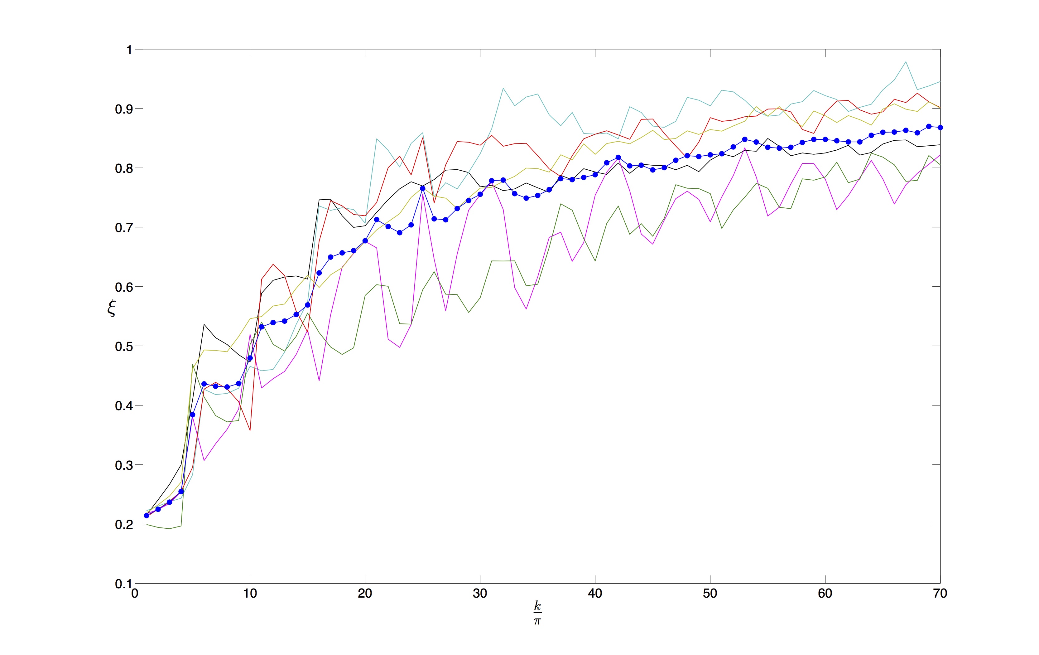
Figure 1: Simulations for $M=25$ modes, showing the mixed-ensemble curve $\xi=\xi(k)$ (in blue with bullets). For comparison we also plot the six ‘pure-ensemble’ curves $\xi_{n}=\xi_{n}(k)$ each obtained from the ratio $(D_{1n}^{2}+D_{2n}^{2})/(\Delta_{1n}^{2}+\Delta_{2n}^{2})$ for a single set of (randomly-chosen) initial phases. The mixed-ensemble curve $\xi(k)$ is more relevant to observation.

3.1 Fixed time interval and varying number of modes

We first consider the mixed-ensemble curve $\xi=\xi(k)$ obtained from evolution over a fixed time interval $(t_{i},t_{f})=(10^{-4},10^{-2})$ and for varying values of $M$. The results are shown in Figure 2, for $M=4,6,9,12,16,20,25$. The curves show some interesting small-scale features. But to a first approximation we may focus on the smooth, overall structure and try fitting to a simple function with no oscillations. (Fits that include oscillations will be considered in Section 3.3.)

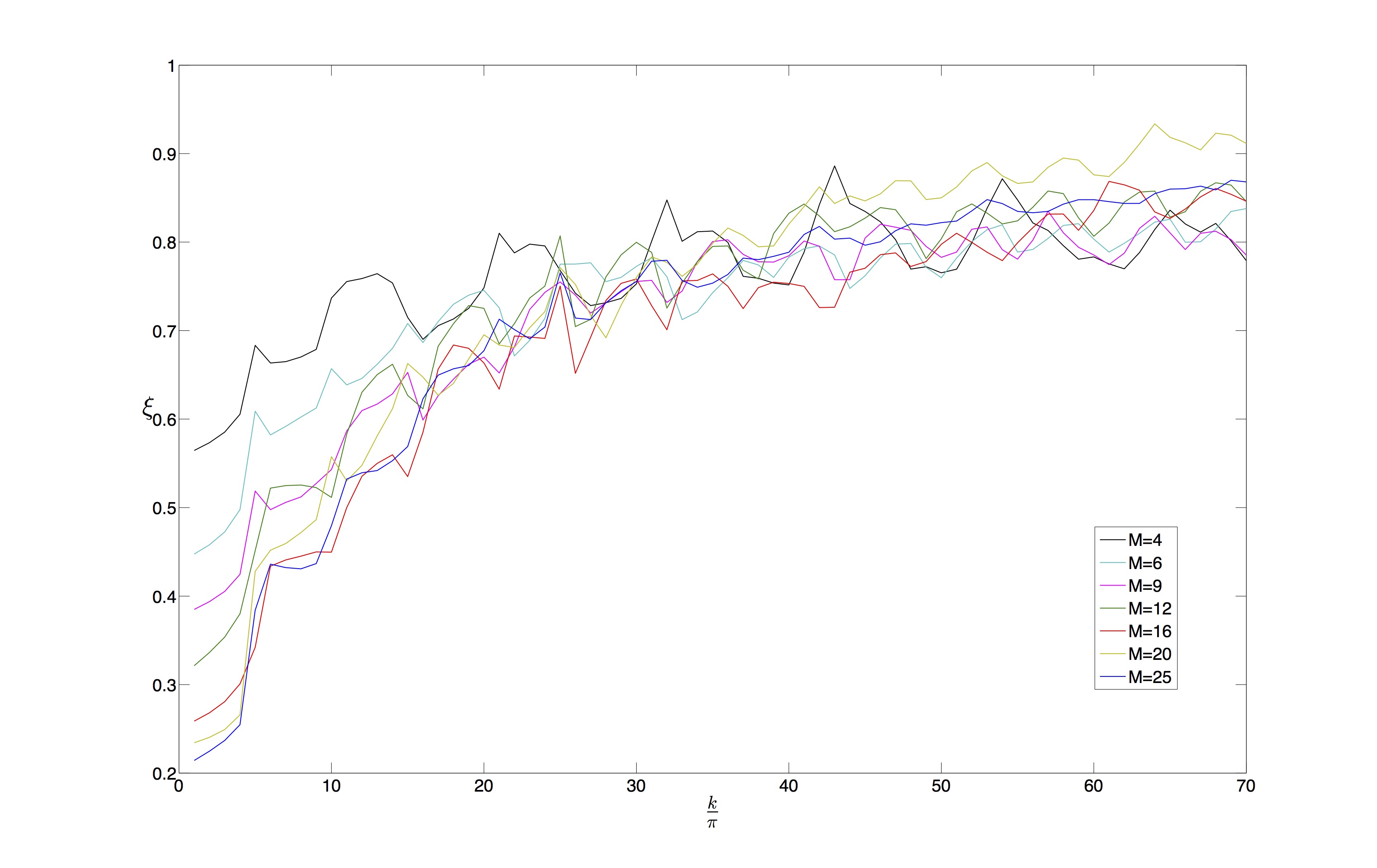
Figure 2: Mixed-ensemble curves $\xi(k)$ for varying $M=4,6,9,12,16,20,25$ with a fixed time interval $(t_{i},t_{f})=(10^{-4},10^{-2})$.

For each $M$ we find a best fit of $\xi(k)$ to the curve

$$\xi(k)=\tan^{-1}(c_{1}\frac{k}{\pi}+c_{2})-\frac{\pi}{2}+c_{3}$$ (22)

where $c_{1}$, $c_{2}$ and $c_{3}$ are free parameters.

Note that $\xi\rightarrow c_{3}$ as $k\rightarrow\infty$. Thus this choice of fitting function includes the possibility that $\xi$ does not approach unity at large $k$ – in which case there will be a residual nonequilibrium $\xi<1$ even in the short-wavelength limit. (For example, for $M=12$ we will find that $c_{3}=0.95$.) Such a residue would in effect induce an overall renormalisation of the observed power spectrum and would therefore in itself not really be observable – or at least not distinguishable from an equivalent shift in other cosmological parameters. For example, in standard models the primordial power spectrum $\mathcal{P}_{\mathcal{R}}^{\mathrm{QT}}(k)$ is to lowest-order proportional to the fourth power of the Hubble parameter $H_{\mathrm{\inf}}$ during inflation, and this parameter is subject to a large uncertainty. We shall see that our residue $c_{3}$ is only slightly less than $1$ and so could easily be offset by a small increase in $H_{\inf}$.

Given the best fits for each $M$, we may study how the parameters $c_{1}$, $c_{2}$ and $c_{3}$ depend on $M$, in the hope of extracting general features.

From Figure 2 we may discern some overall trends: (i) At low $k$ we see that $\xi$ is smaller for larger $M$. This is simply because at low $k$ little evolution has taken place (owing to retardation at long wavelengths) and so the distributions approximate their initial values, where for larger $M$ the initial equilibrium distribution has a larger spread. (ii) There are oscillations in $\xi(k)$. While the oscillations appear regular in some cases (notably $M=4$ and $16$) for others they are rather erratic (for example $M=9$). (iii) At high $k$ there is an approximate convergence of $\xi$ towards $1$.

As one would expect, $\xi$ generally reaches closer to $1$ for larger $M$. (This is expected since for a given time interval there will be more relaxation for larger $M$.) As we shall see presently, the best-fit limiting value $c_{3}$ generally increases for increasing $M$. However, the curve for $M=20$ is in this respect somewhat puzzling, since the corresponding value of $c_{3}$ is found to be significantly larger than for $M=25$ in contradiction with the overall trend. This is clear by eye from Figure 2. The curve for $M=20$ begins approximately mid-way between the curves for $M=16$ and $M=25$, and yet it ends significantly higher than any of the other curves. At present we have no explanation for this seemingly anomalous result for $M=20$. In attempting to extract a general functional dependence for the parameters $c_{1}$, $c_{2}$ and $c_{3}$, we find it convenient to omit the results for $M=20$. Pending further understanding, it seems reasonable to discount this case – especially since, as we shall see, taken on their own the other results mostly follow a clear and simple pattern.

Let us then examine the results of best-fits to the function (22) for $M=4,6,9,12,16,25$ (omitting $M=20$). The results are shown in Figure 3. For each $M$ we display the curve $\xi(k)$ obtained from the simulations together with the best-fit curve. We find good fits to the function (22) on the whole interval $(\pi,70\pi)$, with oscillations around the curve.

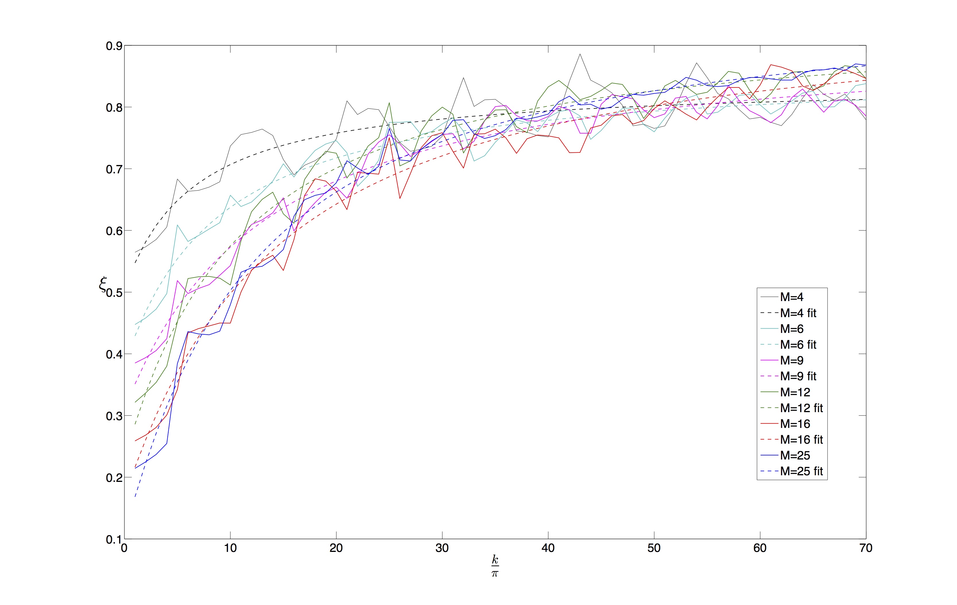
Figure 3: Results for $M=4,6,9,12,16,25$ (omitting the ‘anomalous’ case $M=20$). For each $M$ we plot the curve $\xi(k)$ obtained from simulations (solid line) and the best fit to the function (22) (dashed line).

As is plain from Figure 3, the simulated functions $\xi(k)$ have an oscillatory structure around a smooth curve that is well-approximated by (22). We may then study how the best-fit parameters $c_{1},c_{2},c_{3}$ vary with $M$.

The numerical values obtained for $c_{1},c_{2},c_{3}$ as $M$ varies are listed in Table 1. As $M$ increases, $c_{1}$ and $c_{2}$ decrease more or less monotonically while $c_{3}$ steadily approaches $1$.

$M$	$c_{1}$	$c_{2}$	$c_{3}$
$4$	$0.46$	$2.85$	$0.84$
$6$	$0.24$	$1.91$	$0.86$
$9$	$0.14$	$1.44$	$0.92$
$12$	$0.14$	$1.14$	$0.95$
$16$	$0.10$	$0.97$	$0.97$
$25$	$0.11$	$0.83$	$0.99$

Table 1: Results for the best-fit parameters $c_{1}$, $c_{2}$ and $c_{3}$ for varying $M$ (with the fixed time interval $(t_{i},t_{f})=(10^{-4},10^{-2})$).

Given the best-fit values $c_{1},c_{2},c_{3}$ for varying $M$, we now examine how these values may be fit to simple functions $c_{1}=c_{1}(M)$, $c_{2}=c_{2}(M)$, $c_{3}=c_{3}(M)$.

For $c_{1}$ as a function of $M$ we find a good fit to the curve

$$c_{1}=0.11+2.35e^{-0.48M}\ .$$ (23)

This is shown in Figure 4, which includes data points at $M=4,6,9,12,16,25$ (omitting the ‘anomalous’ case $M=20$).

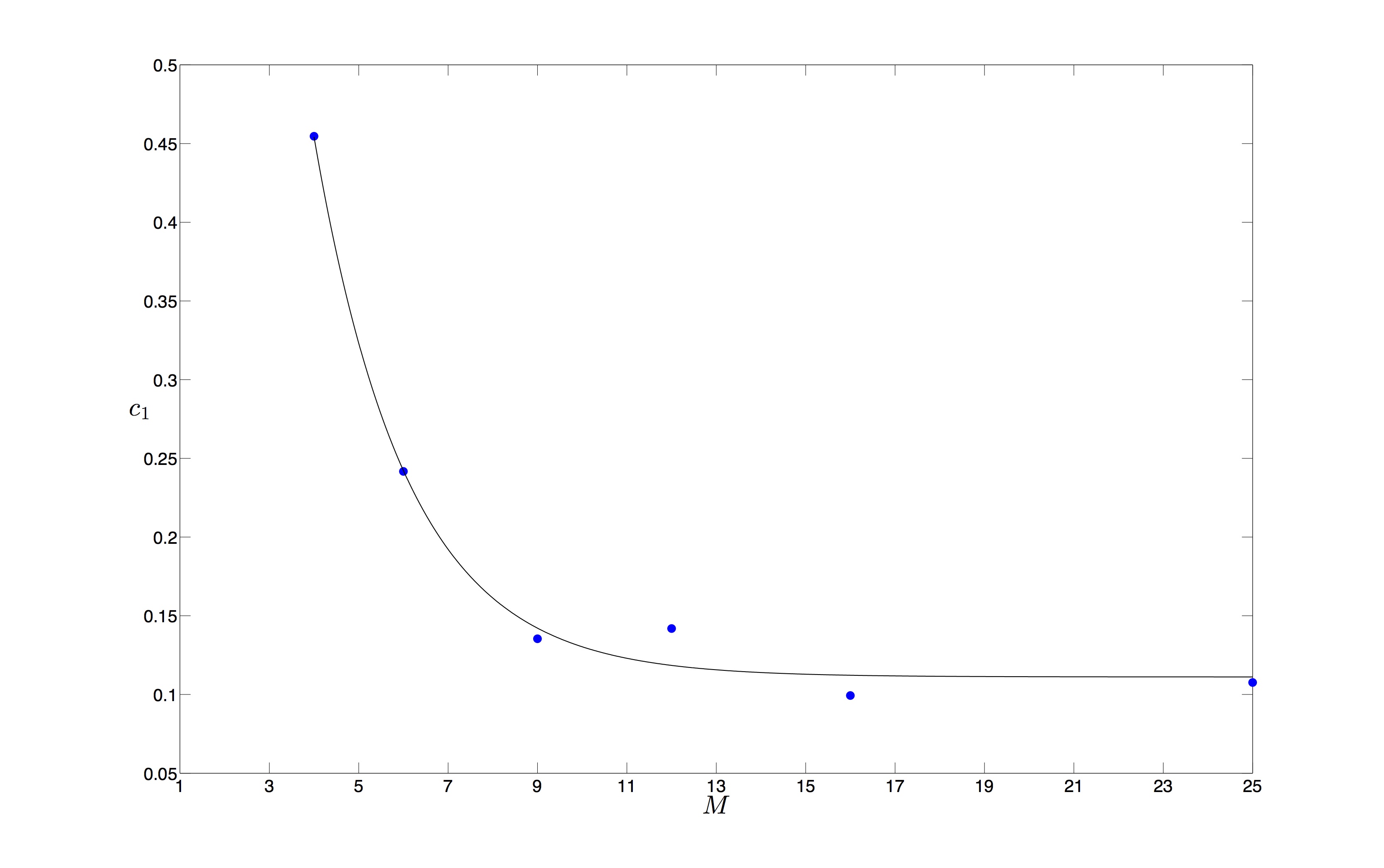
Figure 4: Plot of $c_{1}$ as a function of $M$, with a best-fit curve (23).

For $c_{2}$ as a function of $M$ we find a good fit to

$$c_{2}=0.88+5.67e^{-0.27M}\ .$$ (24)

This is shown in Figure 5, again for $M=4,6,9,12,16,25$.

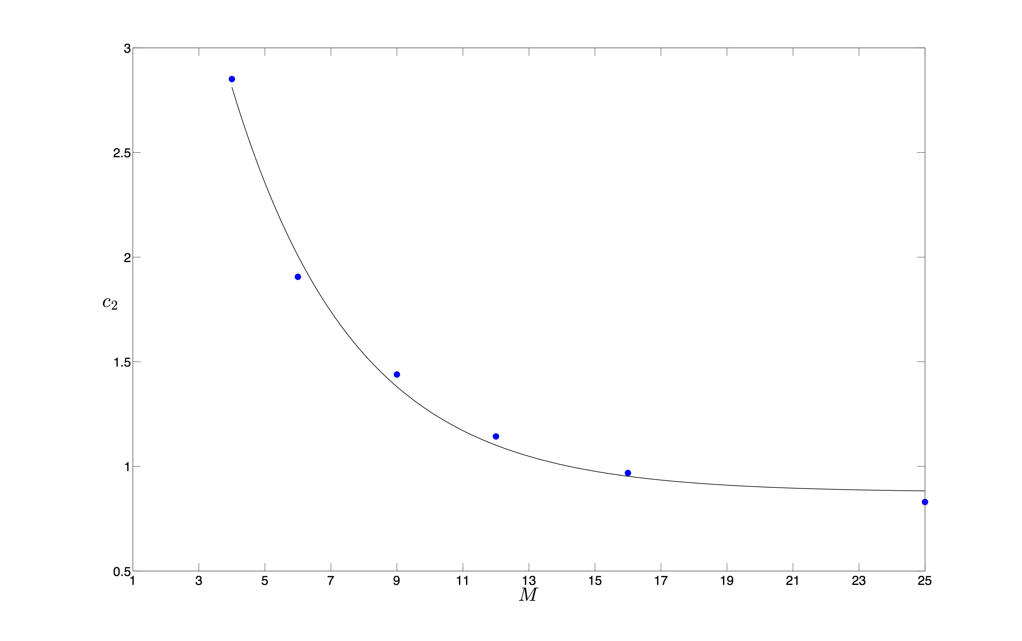
Figure 5: Plot of $c_{2}$ as a function of $M$, with a best-fit curve (24).

Finally, for $c_{3}$ as a function of $M$ we find a good fit to

$$c_{3}=\tan^{-1}(0.53M+2.36)-\frac{\pi}{2}+1.06\ .$$ (25)

This is shown in Figure 6 (for $M=4,6,9,12,16,25$).

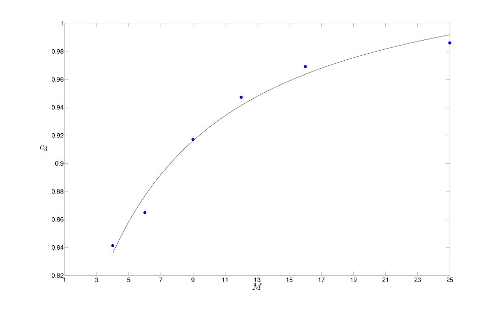
Figure 6: Plot of $c_{3}$ as a function of $M$, with a best-fit curve (25).

As we have noted, the parameter $c_{3}$ is the limiting value (or ‘residue’) of $\xi$ as $k\rightarrow\infty$. According to (25), this parameter in turn has a limiting value $c_{3}\rightarrow c\simeq 1$ as $M\rightarrow\infty$. (The difference of the fitted value $c=1.06$ from $1$ does not seem sufficiently large to be considered significant, given the accuracy of our simulations and of our fits.) It then appears that, as best as we are able to determine, in the limiting regime where the wavenumber and the number of modes are both large we will find that $\xi\simeq 1$ – that is, equilibrium will be obtained to good accuracy, as one expects in a regime with both short wavelengths and large numbers of modes.

One might ask why $c_{3}$ is not equal to $1$ for small values of $M$. The observed behaviour of $c_{3}$ is in fact consistent with what is already known about relaxation. In ref. [43] it was shown that, for a standard two-dimensional harmonic oscillator (which corresponds mathematically to the short-wavelength or large $k$ limit for our field mode on expanding space), if the number $M$ of energy states in the superposition is small then while relaxation takes place to a good approximation it is unlikely to take place completely. This is because the trajectories are unlikely to fully explore the configuration space, resulting in a small ‘residue’ in the coarse-grained $H$-function (indicating a small deviation from equilibrium) even in the long-time limit. Whether or not there is a residue depends on the relative phases in the initial superposition. If these are chosen randomly, then long-time simulations indicate that a nonequilibrium residue is likely to exist for small $M$ and unlikely to exist for large $M$ (see ref. [43] for details). For small $M$, then, we may expect a similar nonequilibrium ‘residue’ in the width of the distribution at large $k$. Thus it may be expected that $c_{3}$ will be slightly less than $1$ (noting that our results are obtained by averaging over mixed states with randomly-chosen initial phases) and that $c_{3}$ will become closer to $1$ for larger $M$ – as indeed is observed in our results (Figure 6).

3.2 Varying time interval and fixed number of modes

We have also performed simulations for $\xi(k)$ with a varying final time $t_{f}$ (the initial time $t_{i}=10^{-4}$ is kept fixed) and with a fixed number $M=12$ of modes. In Figure 7 we display our results for $t_{f}=0.01x$, where $x=1/3,\ 2/3,\ 1,\ 4/3,\ 5/3,\ 2$, together with best-fits to the function (22).

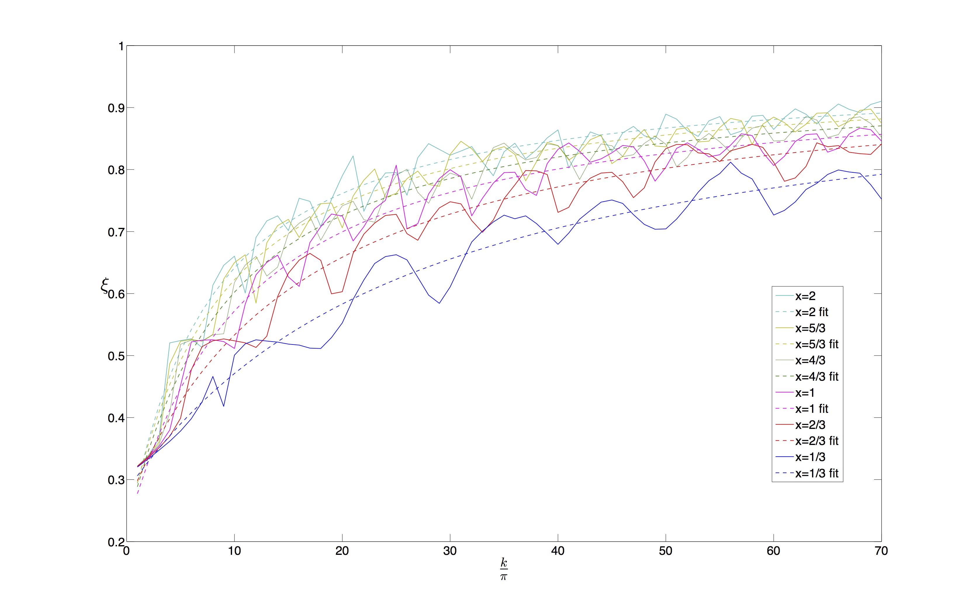
Figure 7: Results for $\xi(k)$ with varying final time $t_{f}=0.01x$ (where $x=1/3,\ 2/3,\ 1,\ 4/3,\ 5/3,\ 2$) and a fixed number $M=12$ of modes. The initial time $t_{i}=10^{-4}$ is kept fixed. Also displayed are best fits to the function (22).

There is again a good fit to the function (22). We see that, as $t_{f}$ increases, $\xi(k)$ increases overall. This is expected, since a longer time interval will in general yield more relaxation for fixed $M$. (As before, to a first approximation we may ignore the oscillations. We note, however, that as $t_{f}$ increases the period of the oscillations decreases.)

The values of the best-fit parameters $c_{1}$, $c_{2}$ and $c_{3}$ for varying $t_{f}$ are shown in Table 2. We see that $c_{1}$ and $c_{2}$ vary significantly with $t_{f}$, while $c_{3}$ is essentially constant.

$t_{f}$	$c_{1}$	$c_{2}$	$c_{3}$
$0.01/3$	$0.06$	$1.21$	$0.97$
$0.02/3$	$0.10$	$1.18$	$0.96$
$0.01$	$0.14$	$1.14$	$0.95$
$0.04/3$	$0.16$	$1.12$	$0.95$
$0.05/3$	$0.18$	$1.11$	$0.96$
$0.02$	$0.20$	$1.08$	$0.96$

Table 2: Best-fit parameters $c_{1}$, $c_{2}$, $c_{3}$ for varying $t_{f}$ (with fixed $t_{i}=10^{-4}$, $M=12$).

In Figure 8 we plot $c_{1}$ as a function of $t_{f}$, together with a best-fit to the curve

$$c_{1}=0.24-0.24e^{-87.16t_{f}}\ .$$ (26)

Note that for $t_{f}=t_{i}$ the curve (26) yields $c_{1}\simeq 0$. This is consistent with the fact that the ‘initial’ ratio $\xi(k)$ – defined as above but with $t_{f}=t_{i}$ – is independent of $k$. Our initial distributions $\rho(q_{1},q_{2},t_{i})$ and $|\psi(q_{1},q_{2},t_{i})|^{2}$ all have variances that are proportional to $1/k$ and so the dependence on $k$ cancels out in the initial ratio $\xi(k)$ (which for $M=12$ is found to be $\simeq 0.3$ for all $k$).

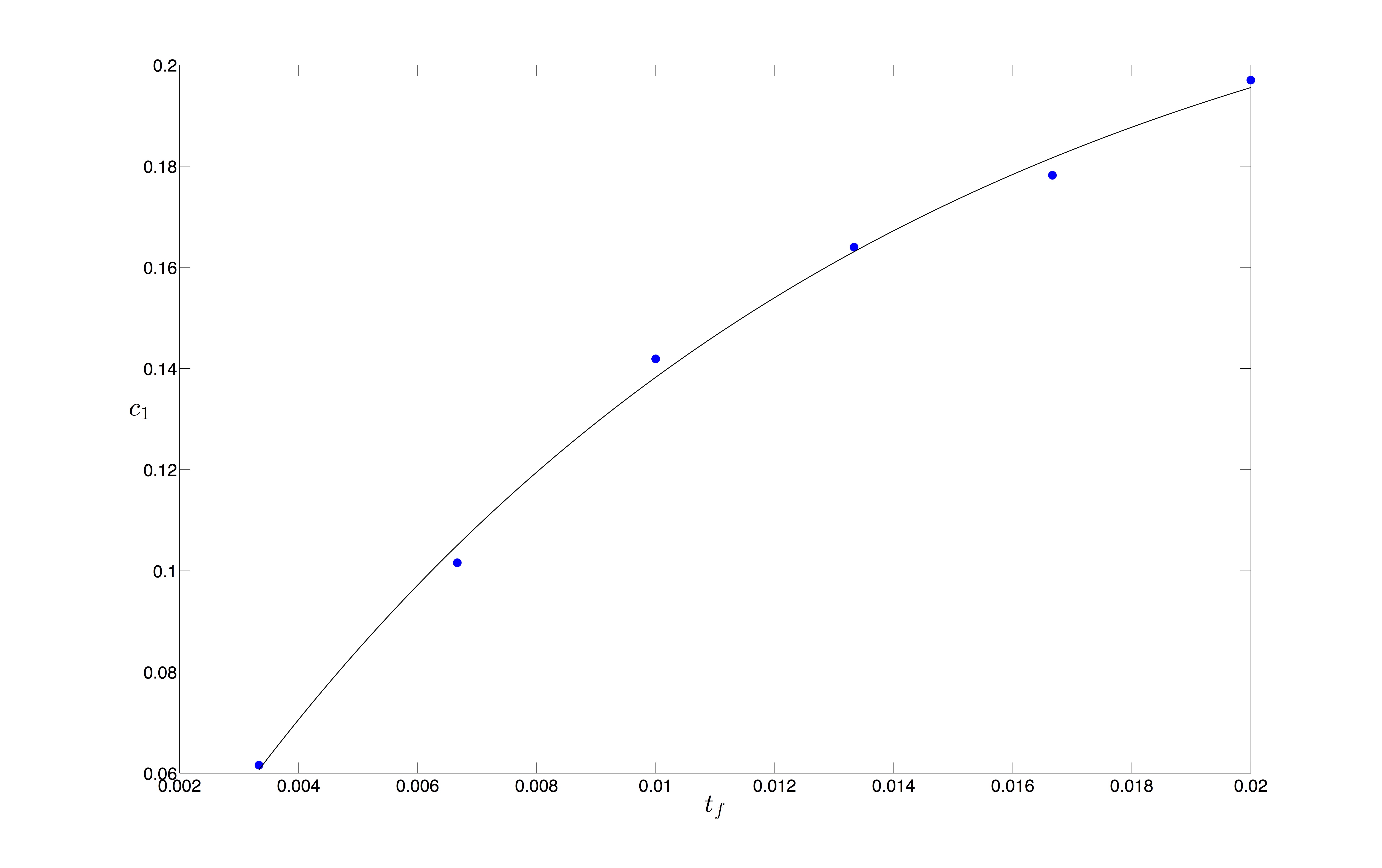
Figure 8: Plot of $c_{1}$ as a function of $t_{f}$, together with a best-fit to the curve (26).

In Figure 9 we plot $c_{2}$ as a function of $t_{f}$, together with a best-fit to the straight line

$$c_{2}=1.23-7.54t_{f}\ .$$ (27)

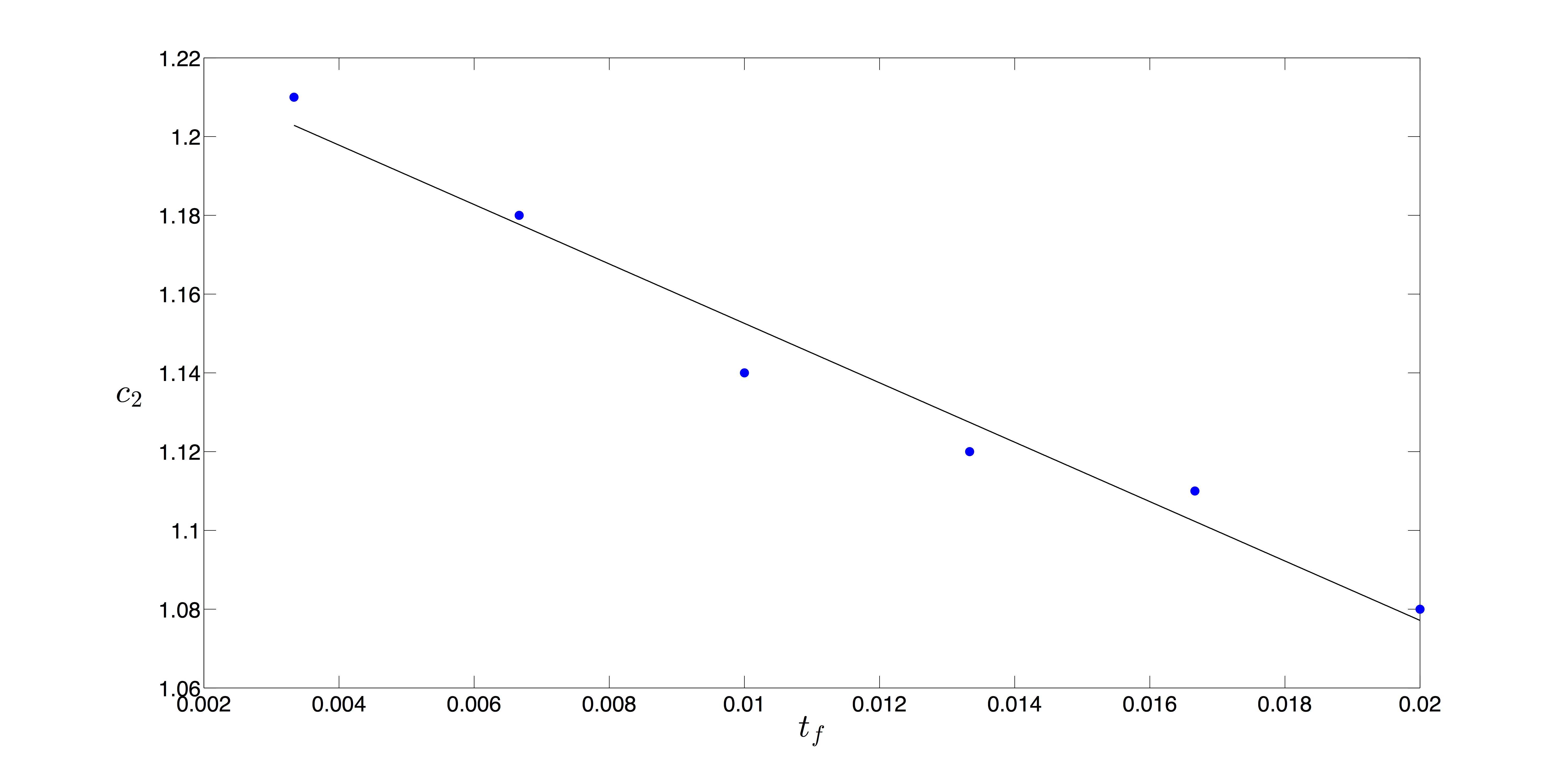
Figure 9: Plot of $c_{2}$ as a function of $t_{f}$, together with a best-fit to the straight line (27).

A fuller exploration of the range of parameters $t_{f}$, $M$ must be left for future work, perhaps with greater computational resources. In the regime studied here, $c_{1}$ and $c_{2}$ depend on both $M$ and $t_{f}$ while $c_{3}$ depends (essentially) only on $M$. We have found best-fit functions $c_{1}=c_{1}(M)$, $c_{2}=c_{2}(M)$, $c_{3}=c_{3}(M)$ (equations (23 ), (24) and (25)) for fixed $t_{f}=10^{-2}$ and $c_{1}=c_{1}(t_{f})$, $c_{2}=c_{2}(t_{f})$ (equations (26) and (27)) for fixed $M=12$. It is evident that we really have a model with two parameters $M$ and $t_{f}$ – assuming a fixed initial time $t_{i}$ and a given initial nonequilibrium distribution (12). However, further simulations that explore the $M-t_{f}$ plane are required to find the best-fit dependence $c_{1}=c_{1}(M,t_{f})$ and $c_{2}=c_{2}(M,t_{f})$, as well as to confirm if $c_{3}$ is essentially independent of $t_{f}$ while varying with $M$. Given the three parameters $c_{1},c_{2},c_{3}$ as functions of $M,t_{f}$, we would then have an explicit two-parameter model for the power deficit.

3.3 Oscillations in the power deficit

Our simulated deficit functions $\xi(k)$ show oscillations. As a first approximation we have ignored these and found fits to the inverse-tangent function (22). Here we attempt to find fits that capture the oscillations as well.

The oscillations in $\xi(k)$ may be related to the retarded time, which has an oscillatory dependence on $k$ (see equations (7)–(9 )). In effect, up to a final time $t_{f}$ our field system evolves like an ordinary oscillator up to a final time $t_{\mathrm{ret}}(t_{f},k)$ that depends on $k$. As $t_{\mathrm{ret}}(t_{f},k)$ rises or falls with varying $k$, we broadly expect a larger or smaller degree of relaxation respectively. Since the ordinary oscillator shows an exponential decay of the coarse-grained $H$-function $\bar{H}(t)$ with time $t$, and since $\xi$ approaches $1$ as the system relaxes, it is heuristically natural to attempt a fit of the form

$$\xi(k)=a-b\exp(-ct_{\mathrm{ret}}(t_{f},k))\ .$$ (28)

Best fits to the function (28) have been performed for varying $M=4,6,9,12,16,20,25$ (with fixed $t_{f}=10^{-2}$). Illustrative results for the cases $M=4,9,16,25$ are shown in Figure 10.

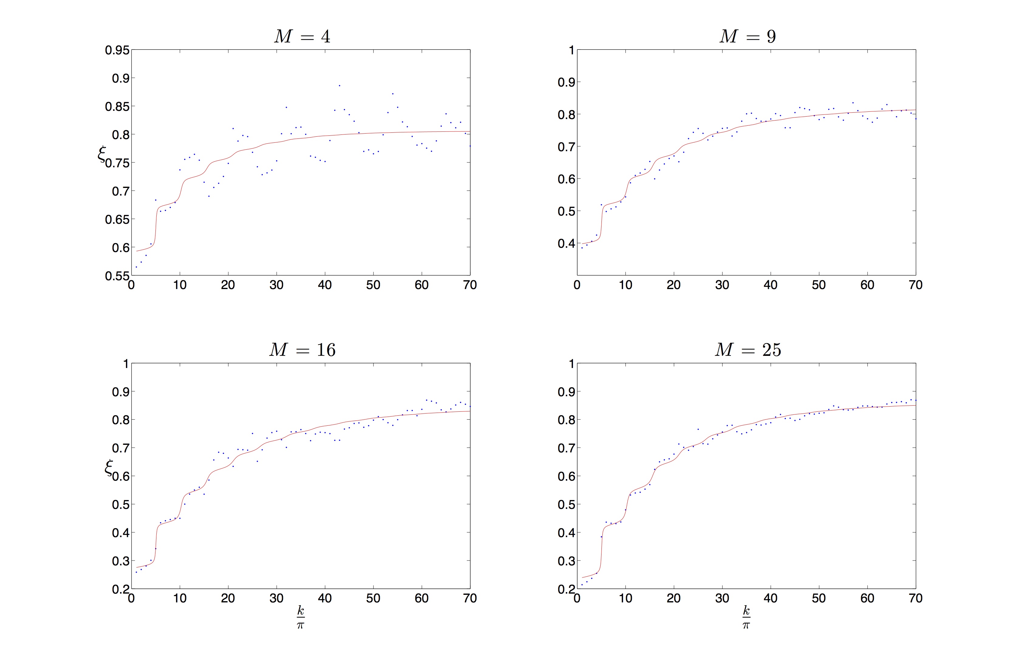
Figure 10: Fitting the oscillations in the power deficit with the exponential function (28) of the retarded time $t_{\mathrm{ret}}(t_{f},k)$ (with varying $M$ and fixed $t_{f}=10^{-2}$).

We see that the fit (28) captures the overall shape of the curve just as well as the inverse-tangent fit (22), while in addition capturing some features of the oscillations in particular at low $k$. The fit to the oscillations is better for larger $M$. However, the fit to the oscillations is poor at very low $M$ (where as we have noted very low $M$ is probably most realistic for the pre-inflationary phase).

As $M$ increases from $M=4$ to $M=25$ (with fixed $t_{f}=10^{-2}$) the best-fit values of $a$, $c$ are roughly constant while $b$ increases monotonically (the case $M=20$ again being an exception, see Table 3).

$M$	$a$	$b$	$c$
$4$	$0.81$	$0.21$	$0.14$
$6$	$0.80$	$0.32$	$0.12$
$9$	$0.82$	$0.42$	$0.10$
$12$	$0.85$	$0.50$	$0.11$
$16$	$0.84$	$0.57$	$0.10$
$20$	$0.92$	$0.64$	$0.09$
$25$	$0.86$	$0.62$	$0.11$

Table 3: Best-fit parameters $a$, $b$, $c$ for the curve (28) (varying $M$ and fixed $t_{f}=10^{-2}$).

In Figure 11 we plot $b$ as a function of $M$ with a best-fit curve

$$b=0.65-0.74\exp(-0.13M)$$ (29)

(omitting the ‘anomalous’ spike at $M=20$).

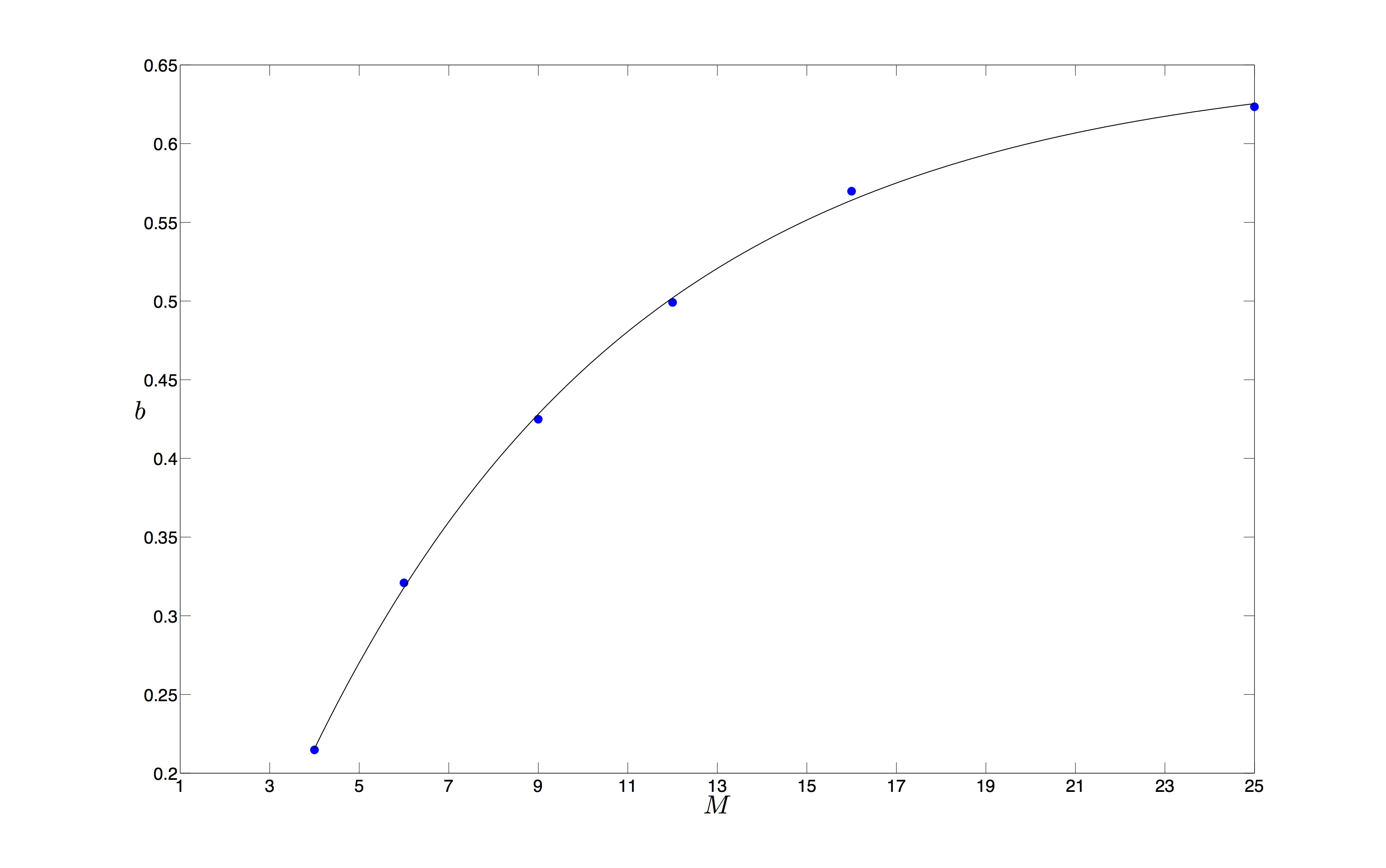
Figure 11: The parameter $b$ as a function of $M$, with a best-fit curve (29).

Best fits to the curve (28) have also been evaluated for varying $t_{f}=0.01x$ where $x=1/3,\ 2/3,\ 1,\ 4/3,\ 5/3,\ 2$ (with fixed $M=12$). The best-fit values of $a$, $b$, $c$ are very nearly constant over this range of $t_{f}$, with $a$ and $b$ steadily increasing by a small fraction while $c$ decreases slightly (see Table 4). Thus to a first approximation $\xi$ depends on $t_{f}$ only via the known function $t_{\mathrm{ret}}(t_{f},k)$. (Note that the expression for $t_{\mathrm{ret}}(t_{f},k)$, as defined by equations (7)–(9), is independent of $M$.)

$t_{f}$	$a$	$b$	$c$
$0.01/3$	$0.83$	$0.47$	$0.12$
$0.02/3$	$0.84$	$0.49$	$0.11$
$0.01$	$0.85$	$0.50$	$0.11$
$0.04/3$	$0.86$	$0.50$	$0.11$
$0.05/3$	$0.87$	$0.52$	$0.10$
$0.02$	$0.88$	$0.52$	$0.10$

Table 4: Best-fit parameters $a$, $b$, $c$ for the curve (28) (varying $t_{f}$ and fixed $M=12$).

We again have a two-parameter model of the power deficit in terms of parameters $M$, $t_{f}$ (again for a fixed initial time $t_{i}$ and a given initial nonequilibrium distribution (12)).

The fit (28) provides an approximate account of the oscillations in $\xi(k)$ for the low-$k$ region. However it does not at all capture the oscillations in $\xi(k)$ for higher $k$, which are especially large for very low $M$. We have tried an alternative fit of the form

$$\xi(k)=\tan^{-1}(c_{1}k/\pi+c_{2})-\pi/2+c_{3}+c_{4}\cos(c_{5}k/\pi)\sin(c_{6}k/\pi)\ ,$$ (30)

which simply adds an oscillatory function to the inverse tangent (22). We find a fairly good fit for $M=4$, as shown in Figure 12, but not for $M=6$ or $M=9$. For the latter cases Fourier analysis shows the presence of additional frequencies. (As we have noted, by eye one sees from Figure 2 that the oscillations in $\xi(k)$ can be rather erratic even if they appear regular for $M=4$.)

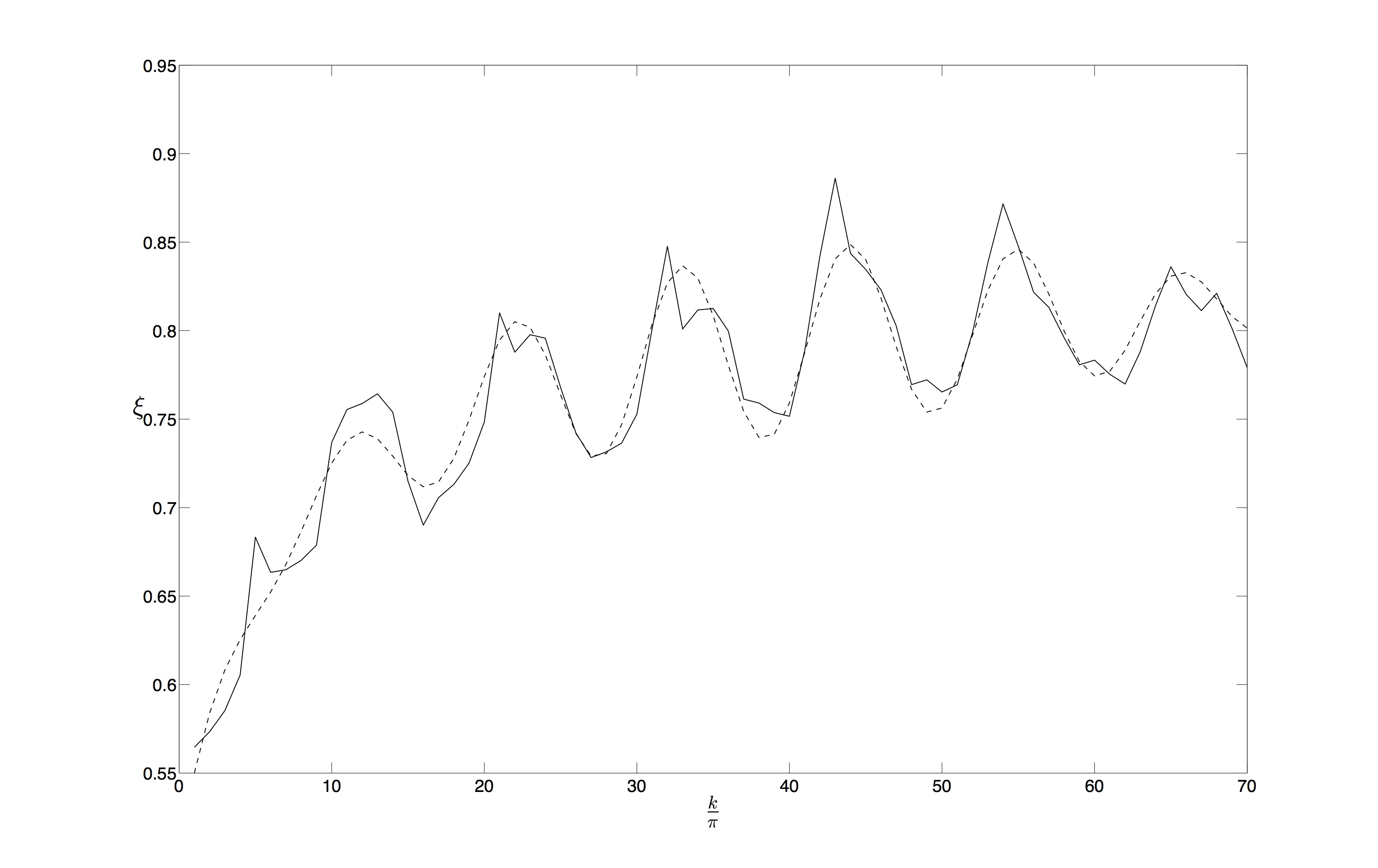
Figure 12: An alternative best-fit curve (30) for the case $M=4$ (with coefficients $c_{1}=0.46$, $c_{2}=2.87$, $c_{3}=0.84$, $c_{4}=0.05$, $c_{5}=0.57$, $c_{6}=0.04$).

A full characterisation of the oscillations is left for future work. However, we may make some general comments. First, oscillations in the large-scale (low-$k$) primordial spectrum appear to be a generic prediction of our model (although further study is required to fully parameterise their features). Second, oscillations in the primordial spectrum also seem to be a generic prediction of models with trans-Planckian corrections to quantum field theory [44]. How these (generally differing) predictions may be compared and distinguished is left for future work. Finally, the overall success of the fit (28) – which performs at least as well as the inverse-tangent fit (22) – suggests that the power deficit will approximately follow this generic form for arbitrary cosmological expansions and not just for a radiation-dominated expansion (where different functions of time for the scale factor $a=a(t)$ will imply different functions for the retarded time $t_{\mathrm{ret}}(t,k)$).

4 Phase relaxation

So far we have studied the nonequilibrium deficit function $\xi(k)$, which measures the deviation of the width of the primordial distribution from the equilibrium value. The observed power deficit at $l\lesssim 40$ might be caused by a dip in $\xi(k)$ at long wavelengths (small $k$).

Also of interest is the distribution of the phase $\theta_{\mathbf{k}}=\tan^{-1}(q_{\mathbf{k}2}/q_{\mathbf{k}1})$ of the Fourier component of the primordial field. The observed anisotropy in the CMB at $l\lesssim 10$ might be caused by nonequilibrium phases at long wavelengths.

As we have noted, statistical isotropy for the CMB implies the standard relations (15). (These might be satisfied, for example, by a Gaussian field with uncorrelated phases.) Isotropy therefore requires that $\left\langle a_{l^{\prime}m^{\prime}}^{\ast}a_{lm}\right\rangle=0$ for all $l,m\neq l^{\prime},m^{\prime}$. However, data from the Planck satellite show evidence for ‘phase correlations’ at low $l$, in the sense that $\left\langle a_{l^{\prime}m^{\prime}}^{\ast}a_{lm}\right\rangle\neq 0$ for some $l,m\neq l^{\prime},m^{\prime}$ at low values of $l,l^{\prime}$ (in the region $l,l^{\prime}\lesssim 10$). The Planck team also report a seemingly anomalous or unlikely mode alignment, as well as various other effects that indicate statistical anisotropy [35].

The reported phase correlations refer to the phases of the complex coefficients $a_{lm}$, and not directly to the phases of the primordial perturbations. From the linear expression (13) for $a_{lm}$ in terms of $\mathcal{R}_{\mathbf{k}}$, it is clear that the phase of a given $a_{lm}$ is in principle related to all of the primordial phases – that is, to the phases of all of the $\mathcal{R}_{\mathbf{k}}$’s or (equivalently) to the phases of all of the $\phi_{\mathbf{k}}$’s. Writing $\phi_{\mathbf{k}}=\left|\phi_{\mathbf{k}}\right|e^{i\theta_{\mathbf{k}}}$, it has been shown that during inflation the phases $\theta_{\mathbf{k}}$ are static along the de Broglie-Bohm trajectories for the inflaton perturbations, so that an initial nonequilibrium distribution for the $\theta_{\mathbf{k}}$’s will remain unchanged during the inflationary era [8]. Thus, if there is an anomalous distribution of primordial phases at the beginning of inflation, this distribution will be preserved in time and transferred to cosmological lengthscales (as occurs with the power deficit). The resulting anomalous phases in the primordial curvature perturbations $\mathcal{R}_{\mathbf{k}}$ will then affect the observed phases of the coefficients $a_{lm}$ in the CMB.

It therefore seems important to study the relaxation of phases during our radiation-dominated expansion, as a model of phase relaxation during a possible pre-inflationary era, with a view to perhaps explaining the observed anisotropy and associated phase correlations in the $a_{lm}$’s.

Thus we now study relaxation for the phases $\theta_{\mathbf{k}}$ associated with our spectator scalar field on a radiation-dominated background. Consider a mode of wave number $k$. We shall calculate the time evolution of the phase marginal $\rho(\theta_{\mathbf{k}},t)$ – that is, of the marginal probability distribution for $\theta_{\mathbf{k}}$ (obtained by integrating over the amplitude $\left|\phi_{\mathbf{k}}\right|$ in the total probability distribution).

For the initial (Gaussian) nonequilibrium distribution (12) the phase marginal is uniform on the unit circle. Whereas for the initial wave function (10) the equilibrium phase marginal is non-uniform. Thus we have a nonequilibrium phase marginal at the initial time $t_{i}=10^{-4}$. We may then calculate the phase marginal at the final time $t_{f}=10^{-2}$ for varying $M$ and $k$.

In Figures 13 and 14 we plot some illustrative results for the final coarse-grained phase marginal $\bar{\rho}(\theta,t_{f})$ together with the final coarse-grained equilibrium marginal $\bar{\rho}_{\mathrm{QT}}(\theta,t_{f})$ (omitting the label ${\mathbf{k}}$), for $M=4$ and $M=25$ respectively, each with varying values of $k$. (The set of initial phases in the wave function is fixed.) By eye one can discern an approximate relaxation as $k$ increases.

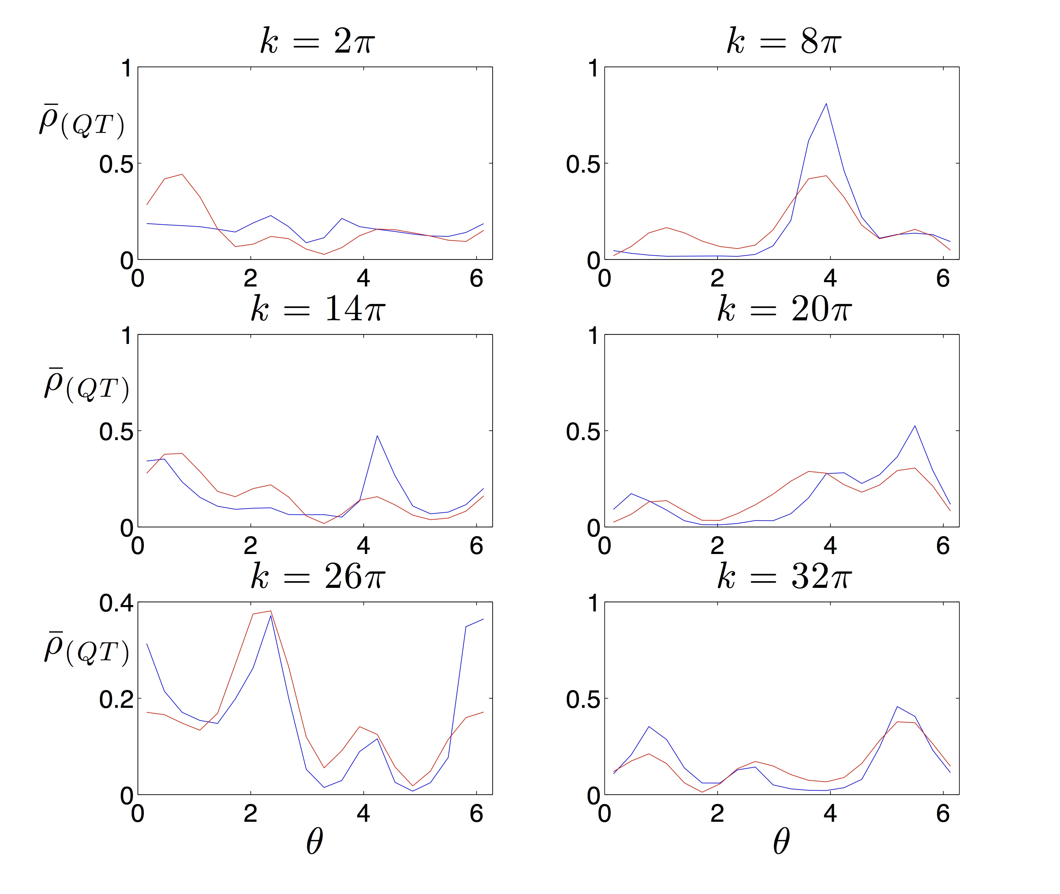
Figure 13: Phase relaxation for $M=4$ (final time $t_{f}=10^{-2}$ and one set of initial phases in the wave function). The blue and red curves are the nonequilibrium and equilibrium distributions respectively.

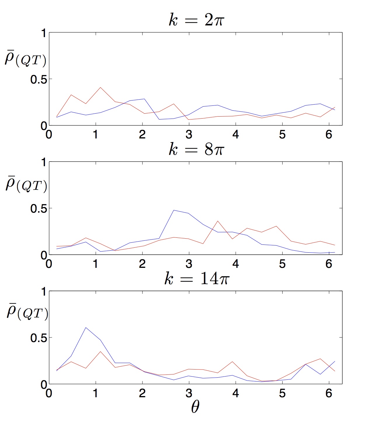
Figure 14: Phase relaxation for $M=25$ (final time $t_{f}=10^{-2}$ and one set of initial phases in the wave function). The blue and red curves are the nonequilibrium and equilibrium distributions respectively.

We must quantify nonequilibrium in a way that is relevant to observations. For amplitudes, observationally what matters is the width of the distribution and so a calculation of $\xi(k)$ suffices. Whereas for phases, observationally what matters is whether they are in quantum equilibrium or not. (For the inflationary vacuum, equilibrium phases are uniformly distributed on $(0,2\pi)$.) To quantify the deviation of the (coarse-grained) phase marginal $\bar{\rho}(\theta,t)$ from the equilibrium marginal $\bar{\rho}_{\mathrm{QT}}(\theta,t)$ we may use the coarse-grained $H$-function

$$\bar{H}_{\theta}(t)=\int d\theta\ \bar{\rho}(\theta,t)\ln\left(\bar{\rho}(\theta,t)/\bar{\rho}_{\mathrm{QT}}(\theta,t)\right)\ .$$ (31)

Thus, while we use $\xi$ as a measure of nonequilibrium for amplitudes, we use $\bar{H}_{\theta}$ as a measure of nonequilibrium for phases.

Of interest here is the process of relaxation towards quantum equilibrium, $\bar{\rho}(\theta,t)\rightarrow\bar{\rho}_{\mathrm{QT}}(\theta,t)$, as quantified by $\bar{H}_{\theta}(t)$. We consider the phase-marginal $H$-function at the final time, $\bar{H}_{\theta}(t_{f})$, for varying $k$ and $M$. Since $t_{f}=10^{-2}$ is fixed, for each $M$ we may regard $\bar{H}_{\theta}$ as a function of $k$. The simulations are run for six sets of initial phases in the wave function. For each $M$ we then obtain six separate curves $\bar{H}_{\theta n}(k)$ (where as before the index $n$ labels the initial wave function corresponding to the choice of initial phases). These may be averaged to yield a mean curve, which we denote by $\bar{H}_{\theta}(k)$. Some illustrative results are shown in Figure 15 for $M=4$, $12$ and $25$, each with $k$ in the range $(\pi,50\pi)$. Many of the curves show an initial increase. Overall, however, there is a general decrease – indicating relaxation – as $k$ increases. (Note that the initial increase is consistent, since the ratio $\bar{\rho}(\theta,t)/\bar{\rho}_{\mathrm{QT}}(\theta,t)$ is not conserved along trajectories for marginals and so the usual $H$-theorem [19] cannot be derived for marginals.)

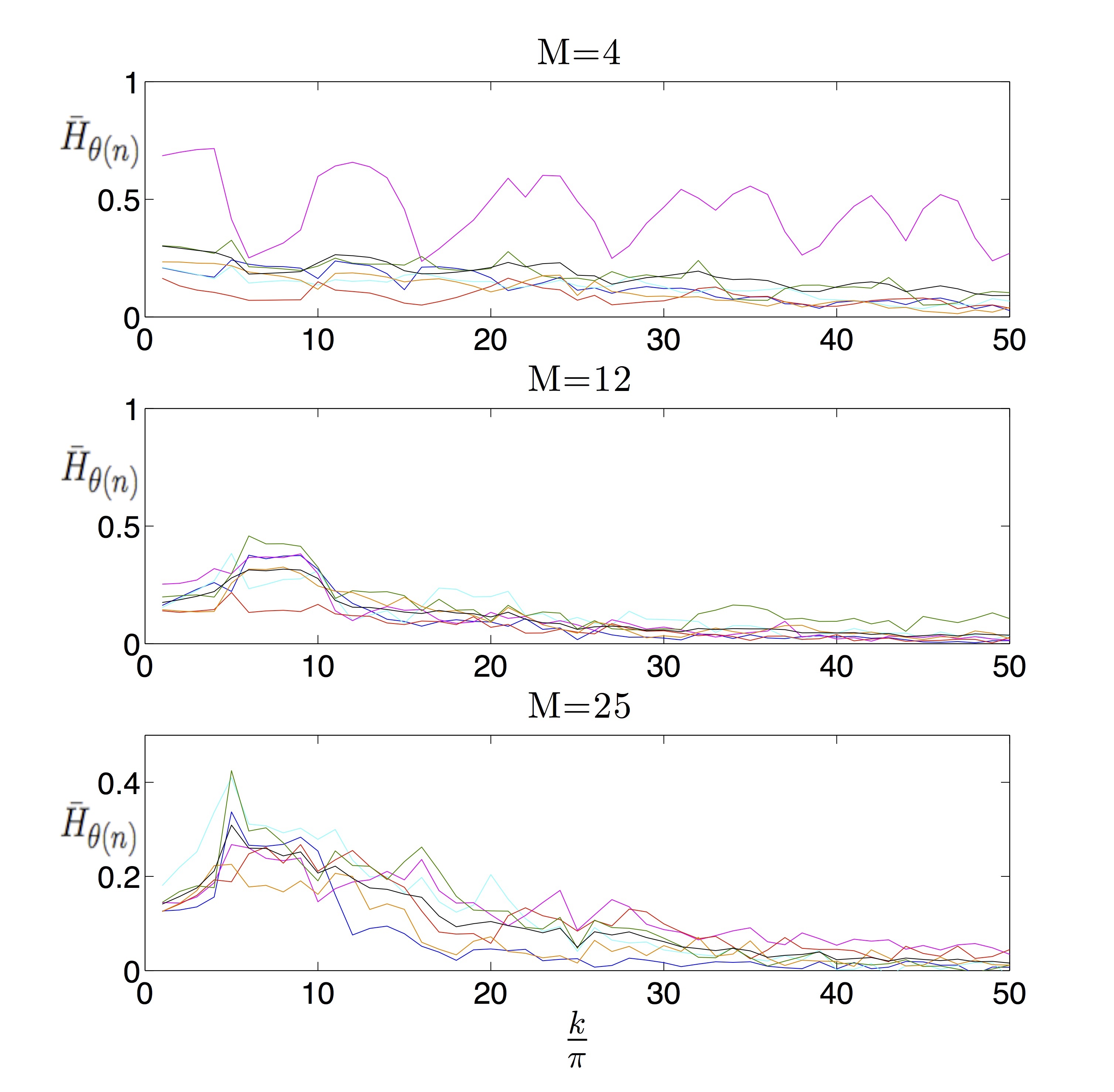
Figure 15: Coarse-grained $H$-functions for final phase marginals, for $M=4,12,25$ (calculated with $t_{f}=10^{-2}$ and six sets of initial phases in the wave function) and for $k$ in the range $(\pi,50\pi)$. The mean curve is shown in black.

5 Relaxation scales for amplitude and phase

For the primordial perturbations we may define two critical $k$-scales, $k_{\mathrm{amp}}$ and $k_{\mathrm{phase}}$, that characterise relaxation for the amplitudes and phases respectively. We shall define $k_{\mathrm{amp}}$ as a value of $k$ below which the amplitudes may roughly be said to have not fully relaxed (so that there is a significant nonequilibrium power deficit). Similarly, we define $k_{\mathrm{phase}}$ as a value of $k$ below which the phases may roughly be said to have not fully relaxed (so that there is a significant departure from quantum randomness). Precise definitions are given below.

The best-fit function (22) for $\xi(k)$ has three parameters $c_{1}$, $c_{2}$ and $c_{3}$. As we noted in Section 3.1, $\xi\rightarrow c_{3}<1$ as $k\rightarrow\infty$, so that $c_{3}$ represents a nonequilibrium residue at short wavelengths. We also found that $c_{3}\simeq 1$ for large $M$. But in a cosmology where the pre-inflationary era contains a small number of modes, we may expect that $c_{3}$ is slightly less than $1$ (indicating a slightly incomplete relaxation even at short wavelengths). Observationally speaking, as already noted in Section 3.1, this would imply an overall renormalisation of the power spectrum, in the sense that the value of $c_{3}$ would be absorbed into effective values for other cosmological parameters (in particular the overall amplitude for the power spectrum). Thus, a residual nonequilibrium $c_{3}<1$ in the power spectrum for large $k$ would not by itself be noticeable. We might, however, notice a dip in the function $\xi(k)$ for small values of $k$. Thus the observable deficit in $\xi$ should be defined relative to the limiting value $c_{3}$.

Let us then define the ‘renormalised’ scale $k_{\mathrm{amp}}$ to be the value of $k$ such that $\xi$ dips significantly below $c_{3}$. For example, we might take

$$\xi(k_{\mathrm{amp}})=0.9c_{3}\;\mathrm{or}\;0.95c_{3}\ .$$ (32)

We shall consider both choices (the exact definition is of course a matter of taste). We denote the resulting values by $k_{\mathrm{amp\ 10\%}}$ and $k_{\mathrm{amp\ 5\%}}$ – corresponding to $10\%$ and $5\%$ (primordial) power deficits respectively.

We consider the $\xi$-curves that were obtained for fixed $t_{f}=10^{-2}$ and varying $M$ (Section 3.1). For these cases the best-fit parameters $c_{1}$, $c_{2}$, $c_{3}$ are listed in Table 1. From (32) we obtain the two values $k_{\mathrm{amp\ 10\%}}$ and $k_{\mathrm{amp\ 5\%}}$ of the characteristic $k$-scale, for each value of $M$ (again omitting the ‘anomalous’ case $M=20$). The results are displayed in Table 5.

$M$	$k_{\mathrm{amp\ 10\%}}$	$k_{\mathrm{amp\ 5\%}}$
$4$	$20\pi$	$46\pi$
$6$	$40\pi$	$88\pi$
$9$	$70\pi$	$150\pi$
$12$	$66\pi$	$141\pi$
$16$	$94\pi$	$198\pi$
$25$	$86\pi$	$181\pi$

Table 5: Results for the $k$-scales $k_{\mathrm{amp\ 10\%}}$ and $k_{\mathrm{amp\ 5\%}}$ for varying $M$ (with the fixed time interval $(t_{i},t_{f})=(10^{-4},10^{-2})$).

The mean $k_{\mathrm{amp}}\equiv\frac{1}{2}(k_{\mathrm{amp\ 10\%}}+k_{\mathrm{amp\ 5\%}})$ lies in the range

$$k_{\mathrm{amp}}\simeq 33\pi-146\pi\ ,$$ (33)

with the lowest values obtained for the lowest $M$ (specifically, $M=4$ and $M=6$).

To define a phase relaxation scale $k_{\mathrm{phase}}$, we may use the mean curve $\bar{H}_{\theta}(k)$ for the coarse-grained phase marginal. While the curve $\bar{H}_{\theta}(k)$ shows an overall decrease with $k$, the dependence is not exponential (see Figure 15). Even so, given an ‘initial’ point $k_{i}$ we may define $k_{\mathrm{phase}}$ by

$$\bar{H}_{\theta}(k_{i}+k_{\mathrm{phase}})=(1/e)\bar{H}_{\theta}(k_{i})$$ (34)

(as one would if $\bar{H}_{\theta}$ were decaying exponentially on a characteristic scale $k_{\mathrm{phase}}$).

Again focussing on the case of fixed $t_{f}=10^{-2}$ and varying $M$, we have performed simulations for $M=4,12,16,20,25$ (each with six sets of initial phases). For each $M$ we obtain an averaged curve $\bar{H}_{\theta}(k)$, from which we may obtain a characteristic scale $k_{\mathrm{phase}}$ defined by (34) (we take $k_{i}=\pi$). The results are: $k_{\mathrm{phase}}=38\pi$, $25\pi$, $43\pi$, $32\pi$, $25\pi$ for $M=4,12,16,20,25$ respectively. Approximately, we find

$$k_{\mathrm{phase}}\simeq 35\pi$$ (35)

(varying with $M$ by about $30\%$).

Thus we find a ratio approximately in the range

$$\frac{k_{\mathrm{phase}}}{k_{\mathrm{amp}}}\simeq\allowbreak 0.2-\allowbreak 1.1\ ,$$ (36)

with the highest values obtained for the lowest $M$ (again $M=4$ and $M=6$).

Roughly speaking, primordial perturbations on a scale $k$ affect the CMB at a multipole $l\simeq(2/H_{0})k$ (where $H_{0}$ is the Hubble parameter today) [1]. If we define analogous quantities $l_{\mathrm{amp}}$ and $l_{\mathrm{phase}}$ as those values of $l$ below which we observe a power deficit and phase anomalies respectively, then we should find a ratio $l_{\mathrm{phase}}/l_{\mathrm{amp}}\simeq k_{\mathrm{phase}}/k_{\mathrm{amp}}$ or

$$\frac{l_{\mathrm{phase}}}{l_{\mathrm{amp}}}\simeq 0.2-\allowbreak 1.1\ .$$ (37)

The Planck data indicate values (roughly) of $l_{\mathrm{phase}}\simeq 10$ and $l_{\mathrm{amp}}\simeq 40$, with a ratio

$$\frac{l_{\mathrm{phase}}}{l_{\mathrm{amp}}}\simeq 0.25\ .$$ (38)

This seems reasonably consistent with our rough estimate (37).

6 Angular power deficit

Let us study more precisely how the proposed deficit in the primordial power spectrum could yield the reported deficit in the angular power spectrum at low $l$.

At low $l$ the (square of the) transfer function takes the form [1]

$$\mathcal{T}^{2}(k,l)=\pi H_{0}^{4}j_{l}^{2}(2k/H_{0})\ .$$ (39)

As a first approximation let us assume that the quantum-theoretical primordial spectrum $\mathcal{P}_{\mathcal{R}}^{\mathrm{QT}}(k)$ is scale invariant. From (16) and (19) we then have an approximate ratio

$$\frac{C_{l}}{C_{l}^{\mathrm{QT}}}=2l(l+1)\int_{0}^{\infty}\frac{dk}{k}\ j_{l}^{2}(2k/H_{0})\xi(k)$$ (40)

(where $C_{l}^{\mathrm{QT}}$ is the quantum-theoretical angular power spectrum). A low power anomaly $C_{l}/C_{l}^{\mathrm{QT}}<1$ in the CMB may be explained by an appropriate primordial deficit $\xi(k)<1$ [8, 13].

If the primordial deficit takes the inverse-tangent form (22), we may evaluate the expression (40) numerically to find the range of parameters $c_{1}$, $c_{2}$, $c_{3}$ giving an angular power deficit in the (crudely speaking) observed range $\sim 5-10\%$ – that is, giving a ratio $C_{l}/C_{l}^{\mathrm{QT}}$ in the range $0.9-0.95$. (Of course the deficit reported by the Planck team is a statistical aggregate for the whole low-$l$ region and does not refer to individual multipoles, so this is only a rough characterisation of the data.)

It is convenient to use the variable $x\equiv 2k/H_{0}$ and to define a rescaled coefficient

$$\tilde{c}_{1}\equiv(H_{0}/2\pi)c_{1}\ .$$ (41)

We then have

$$\frac{C_{l}}{C_{l}^{\mathrm{QT}}}=2l(l+1)\int_{0}^{\infty}\frac{dx}{x}\ j_{l}^{2}(x)\left(\tan^{-1}(\tilde{c}_{1}x+c_{2})-\frac{\pi}{2}+c_{3}\right)$$ (42)

(where $j_{l}^{2}(x)$ is dominated by the scale $x\simeq l$). We have evaluated this expression numerically at low $l$ for varying values of $\tilde{c}_{1}$, $c_{2}$ but keeping $c_{3}$ fixed at $c_{3}=1$. Our results are trivially extended to arbitrary $c_{3}$, since writing $c_{3}=1+(c_{3}-1)$ the expression (42) takes the form

$$C_{l}/C_{l}^{\mathrm{QT}}=\left(C_{l}/C_{l}^{\mathrm{QT}}\right)_{c_{3}=1}+(c_{3}-1)$$

where we have used $\int_{0}^{\infty}\frac{dx}{x}\ j_{l}^{2}(x)=1/2l(l+1)$.

Plots of the calculated deficit $C_{l}/C_{l}^{\mathrm{QT}}$ on the parameter space $(\tilde{c}_{1},c_{2})$ are displayed in Figure 16 for $l=10,14,18,22,26,30$. The green region corresponds to $C_{l}/C_{l}^{\mathrm{QT}}$ in the range $0.9-0.95$. (The blue region corresponds to $C_{l}/C_{l}^{\mathrm{QT}}<0.9$ while the red region corresponds to $C_{l}/C_{l}^{\mathrm{QT}}>0.95$.) The green ‘deficit region’ has parameters $\tilde{c}_{1}$ in the approximate range $[0,1.5]$ and $c_{2}$ in the approximate range $[0,20]$ (restricting ourselves to $\tilde{c}_{1},c_{2}>0$).

Of course we have not performed a best-fit, we have simply obtained the magnitudes that $\tilde{c}_{1}$ and $c_{2}$ must have in order for the low-$l$ angular spectrum to drop by $5-10\%$.

Figure 16: Parameter space $(\tilde{c}_{1},c_{2})$ for $l=10,14,18,22,26,30$. The green regions have $C_{l}/C_{l}^{\mathrm{QT}}$ in the range $0.9-0.95$; the blue regions have $C_{l}/C_{l}^{\mathrm{QT}}<0.9$; the red regions have $C_{l}/C_{l}^{\mathrm{QT}}>0.95$. (Each plot uses $20\times 20$ grid points.)

7 Comparing with observation

Let us now compare the required ranges for $\tilde{c}_{1},c_{2}$ – as deduced from the required angular power deficits – with the results for $c_{1},c_{2}$ obtained from our model. (We will not consider $c_{3}$ here as it may be reabsorbed into an overall renormalisation of the primordial power spectrum.)

To relate our results to observable quantities, we must take into account the spatial expansion by a factor

$$R\equiv\frac{a(t_{\mathrm{today}})}{a(t_{f})}$$ (43)

that will have taken place from the end of pre-inflation at time $t_{f}$ until today at time $t_{\mathrm{today}}$. The true coefficient $c_{1}$ (or $\tilde{c}_{1}$) that appears in the observable power spectrum is then multiplied by the unknown number $R$.

Let us consider this last point more carefully. In our simulations we used natural units ($\hbar=c=1$) with fiducial initial and final times $t_{i}=10^{-4}$, $t_{f}=10^{-2}$. For convenience we also took $a_{0}=1$ at $t_{0}=1$. This means that in our simulations – which yielded a deficit function $\xi(k)$ of the form (22) – $k$ was the physical wavenumber at time $t=t_{0}=1$ (in our units). During the simulated pre-inflationary era we have $a(t)=a_{0}(t/t_{0})^{1/2}=t^{1/2}$ and so (as already noted) at the end of pre-inflation our scale factor is $a_{f}=t_{f}^{1/2}=0.1$. Thus physical wavenumbers at the final time $t_{f}$ are ten times larger than the physical wavenumbers $k$ referred to in our simulations. It follows that physical wavenumbers today, which we might temporarily denote as $k_{\mathrm{today}}$, are given by

$$k_{\mathrm{today}}=(10/R)k\ .$$ (44)

Now, if we assume that our simulated deficit function $\xi(k)$ survives the transition to inflation and indeed provides a correction to the inflationary power spectrum, then the same deficit will enter as a factor in the spectrum of primordial perturbations. It follows that the true correction $\xi_{\mathrm{today}}(k_{\mathrm{today}})$ multiplying the observable primordial spectrum will be

$$\xi_{\mathrm{today}}(k_{\mathrm{today}})=\left[\xi(k)\right]_{k=(R/10)k_{\mathrm{today}}}$$ (45)

(since the mode which we today label $k_{\mathrm{today}}$ was the mode labelled $k=(R/10)k_{\mathrm{today}}$ in our simulations). We may then drop the subscript ‘today’ and simply write the true deficit correction as $\xi(k)$ with $k$ now denoting physical wavenumbers today (as is more conventional). In other words, the true correction multiplying the observable primordial spectrum will be numerically equal to our simulated function $\xi(k)$ but with $k$ replaced by $(R/10)k$ and with $k$ then reinterpreted as the physical wavenumber today. With this understanding, we obtain a true deficit function

$$\xi(k)=\tan^{-1}(\tilde{c}_{1}x+c_{2})-\frac{\pi}{2}+c_{3}$$ (46)

with $x=2k/H_{0}$ and

$$\tilde{c}_{1}\equiv c_{1}RH_{0}/20\pi\ .$$ (47)

Thus the deficit in the angular power spectrum will still take the form (42) but with an observed coefficient $\tilde{c}_{1}$ given by (47), where $c_{1}$ is the coefficient generated by our numerical simulations of the pre-inflationary era (using our convenient units).

We have seen that our simulations yield (to a first approximation) coefficients $c_{1}$ and $c_{2}$ that depend on both $M$ and $t_{f}$ and a coefficient $c_{3}$ that depends only on $M$. The observable spectra will be sensitive to $c_{1}$ via the factor $c_{1}R$ appearing in (47), and so uncertainty in $M$ and $t_{f}$ (and hence in $c_{1}$) is compounded with uncertainty in $R$. On the other hand, the spectra are (at least in principle) directly sensitive to $c_{2}$, $c_{3}$ – which are determined by the dynamics of our model (for a given number $M$ of pre-inflationary excited states and for a given duration $(t_{i},t_{f})$, and assuming the simple initial nonequilibrium distribution (12)). The spectra are also in principle directly sensitive to the inverse-tangent functional form of $\xi(k)$, a feature that is again determined by the dynamics of our model and which seems to be a robust prediction for a fairly broad range of parameters $(t_{f},M)$ characterising the pre-inflationary era. Our simulations also predict phase anomalies at comparable values of $k$, though the implications of this for observable quantities (such as signatures of anisotropy) remain to be explored.

We are unable to predict $R$, but it is subject to well-known constraints. Should $R$ be too large, the effective coefficient $\tilde{c}_{1}$ as given by (47) could be so large that our deficit function (46) appearing in (42) will be essentially equal to the constant $c_{3}$ and will therefore simply generate an overall renormalisation of the power spectrum. If more interesting features of $\xi(k)$ are to be observable, we must assume that the value of $\tilde{c}_{1}$ is such that the $k$-dependence of $\xi(k)$ occurs in an observable range of $k$-space. If we are fortunate and this is correct, we will then be able to test the other (predicted) details of the function $\xi(k)$ – its functional dependence on $k$, and the values of the other two coefficients $c_{2}$, $c_{3}$.

The first thing to check is whether or not our model can yield the required angular power deficit – with $C_{l}/C_{l}^{\mathrm{QT}}$ within the ‘green zone’ of Figure 16 – for reasonable values of the expansion factor $R$. It suffices to find an example of our predicted coefficients $c_{1}$, $c_{2}$ (for some pair of parameters $t_{f}$, $M$) that corresponds to the observed deficit region for an acceptable choice of cosmological parameters.

Our simulations with fixed $t_{f}=10^{-2}$ and varying $M$ (Section 3.1) yielded $c_{1}$ in the range $[0.10,0.46]$ and $c_{2}$ in the range $[0.83,2.85]$. Let us consider the ‘preferred’ case with the smallest number $M=4$ of excited states, which yielded $c_{1}=0.46$ and $c_{2}=2.85$ (see Table 1). If we could take $\tilde{c}_{1}\simeq 0.5$ then from Figure 16 we see that the point $(\tilde{c}_{1},c_{2})\simeq(0.5,2.85)$ would lie in or close to the green zone for all the displayed multipoles $l$. To obtain $\tilde{c}_{1}\simeq 0.5$ when $c_{1}=0.46$ requires (from (47)) $RH_{0}/20\pi\sim 1$. Now our coefficient $c_{1}$ has conventional units of length, or mass dimension $-1$ in natural units, and so our numerical values $c_{1}=x$ must be multiplied by $\hbar c$ to obtain values $c_{1}\simeq(3\times 10^{-24}\ \mathrm{cm})x$ in conventional units. Thus our requirement $RH_{0}/20\pi\sim 1$ is really $(3\times 10^{-24}\ \mathrm{cm})RH_{0}/20\pi\sim 1$ or

$$R\sim 10^{53}$$ (48)

(where $H_{0}^{-1}\simeq 10^{28}\ \mathrm{cm}$).

Is (48) consistent with known cosmological constraints? To see that it is, let us write $R$ as

$$R\equiv a_{\mathrm{today}}/a_{f}=(a_{\mathrm{today}}/a_{\mathrm{end}})(a_{\mathrm{end}}/a_{f})\ ,$$

where $a_{\mathrm{end}}$ is the scale factor at the end of inflation. We may neglect the expansion that takes place during the transition (from pre-inflation to inflation) compared to the expansion that takes place during inflation. Thus we may approximately identify $a_{f}$ with the scale factor $a_{\mathrm{begin}}$ at the beginning of inflation. We then have $a_{\mathrm{end}}/a_{f}\simeq e^{N}$ where $N$ is the number of inflationary e-folds. Let us similarly neglect the expansion that takes place during the transition from inflation to post-inflation. We can then write $a_{\mathrm{today}}/a_{\mathrm{end}}\simeq T_{\mathrm{end}}/T_{\mathrm{today}}$ (where $T_{\mathrm{end}}$ is the temperature at which inflation ends). We then find

$$R\simeq e^{N}(T_{\mathrm{end}}/T_{\mathrm{today}})\ .$$ (49)

The value of the reheating temperature $T_{\mathrm{end}}$ depends on the details of the reheating process. (See for example refs. [4, 49].) We certainly have an upper bound $T_{\mathrm{end}}\lesssim T_{f}$, where $T_{f}$ is the temperature at the end of pre-inflation. Indeed we could even have $T_{\mathrm{end}}<<T_{f}$. We may expect $T_{f}$ to be comparable to the energy scale $H_{\mathrm{\inf}}\sim 10^{16}\ \mathrm{GeV}$ of inflation (where $H_{\mathrm{\inf}}$ is the Hubble parameter during inflation). Thus we may safely write an upper bound $T_{\mathrm{end}}\lesssim 10^{16}\ \mathrm{GeV}$. Lower bounds on $T_{\mathrm{end}}$ in the range $390\ \mathrm{GeV}-890\ \mathrm{TeV}$ (depending on the inflationary model) have been obtained from CMB data [50]. Thus we may take a rough lower bound $T_{\mathrm{end}}\gtrsim 1\ \mathrm{TeV}$. We then have $10^{16}<T_{\mathrm{end}}/T_{\mathrm{today}}<10^{29}$ (where $T_{\mathrm{today}}\sim 10^{-4}\ \mathrm{eV}$), which from (49) implies the bounds $10^{16}e^{N}<R<10^{29}e^{N}$. Our condition (48) then implies a range

$$55<N<85\ .$$ (50)

This is compatible with standard constraints, which indicate that the minimum number $N=N_{\min}$ of e-folds (required for inflation to solve the horizon and flatness problems) is $N_{\min}\simeq 70$ – with some authors taking $N_{\min}\simeq 60$. See, for example, ref. [4]. (The actual number $N$ of e-folds could of course be much larger than $N_{\min}$. As we have noted, if $N$ is too large then the power deficit generated by our model would exist at wavelengths too large to be observable.) Thus there exist acceptable values for the cosmological parameters $N$, $T_{\mathrm{end}}$ such that (48) is satisfied, in which case the simulated coefficients $c_{1}=0.46$, $c_{2}=2.85$ will be consistent with the observed deficit (corresponding to the green zone of Figure 16).

We conclude that the range of values for $c_{1}$, $c_{2}$ required by observation is compatible with the range of values for $c_{1}$, $c_{2}$ obtained from our relaxation simulations. Thus we may say that our model seems viable – pending a full treatment of the transition to inflation.

8 Conclusion

Primordial quantum relaxation provides a single mechanism that can generate both a power deficit and anomalous phases at large angular scales in the CMB. Our estimates show that, with an appropriate choice of cosmological parameters, our model is able to generate a power deficit at approximately the angular scales and of approximately the magnitude that has been reported by the Planck team, as well as generating anomalous phases at comparable angular scales. In addition, the same mechanism generates oscillations in the primordial spectrum.

There are of course other mechanisms that can produce a large-scale power deficit, such as a suitable period of inflationary ‘fast rolling’ [51]. It is hoped that the particular form of our power deficit $\xi(k)$, given by (46) as a function of wavenumber $k$, will distinguish it from the deficit predicted by alternative models.

From the viewpoint of our underlying model, it must be assumed that the number of inflationary e-folds is not too large, for otherwise our effects would exist at wavelengths that are too large to be detectable. On the other hand, once this assumption is made our model makes several clear and testable predictions: an inverse-tangent correction $\xi(k)$ to the large-scale primordial spectrum, with oscillations around the curve, and with anomalous phases at comparable scales. Of the three parameters $\tilde{c}_{1}$, $c_{2}$, $c_{3}$ appearing in our fit (46), the first depends on the number $N$ of inflationary e-folds and on the inflationary reheating temperature $T_{\mathrm{end}}$; but the second and third are entirely determined by our model. The parameters $\tilde{c}_{1}$, $c_{2}$, $c_{3}$ depend on the final time $t_{f}$ and the number $M$ of excited energy states (both defined for the pre-inflationary era). An alternative fit (28), involving an exponential of the retarded time $t_{\mathrm{ret}}(t_{f},k)$, provides an equally good fit to the overall shape of the curve while also capturing some features of the oscillations in the low-$k$ region.

In effect, then, we have a model of the power deficit in terms of two parameters $t_{f}$, $M$ – for a given initial time $t_{i}$ and a given initial nonequilibrium distribution (12). The model generates some rather complex features: a power deficit of a particular form, with oscillations around the curve and with anomalous phases. The prospects are therefore good for a comparison with data. It is of course quite possible that the number of inflationary e-folds is so large that, even if our effects exist, they will be too faint to be observable. But if the effects are visible, they should show detailed signatures.

In this paper we have assumed a fixed initial nonequilibrium distribution (12), equal to the equilibrium distribution for the ground state of the field mode. This was chosen as a simple example of a nonequilibrium distribution whose initial width is smaller than the initial quantum width. One may ask to what extent our final results depend on this choice. We may reasonably expect to find similar results if the initial nonequilibrium distribution is a simple smooth function whose width is smaller than the quantum width (for example, a function equal to the equilibrium distribution associated with a superposition of $M^{\prime}<M$ energy states). For the erratic motion of the trajectories is likely to erase any dependence on the finer details of the initial distribution. We are after all only concerned with the final width – other details of the final distribution do not affect our calculation of the power deficit. We may therefore expect that our results will depend mainly on the initial width only, and not on other details of the initial distribution. This expectation is confirmed by further simulations, in which the initial nonequilibrium distribution includes terms that in quantum equilibrium would result from the first excited state of the field mode. We have found that, while the details of the final distribution are slightly different, the final power deficit has the same inverse-tangent dependence on wavelength as before (with slightly different best-fit parameters). These further simulations will be reported elsewhere, in a separate publication in which we also study the effect of the transition [52].

The extent to which the data support our model remains to be seen. A first step would be to evaluate likelihoods for corrections to the power spectrum of the form (46) [53]. The class of models to be fitted will include the standard cosmological parameters together with our extra parameters. A second step would be to evaluate the extent to which our predicted oscillations are present in the data. Finally, one may also consider in more detail the apparent large-scale anisotropy in the CMB and how it might be explained by the anomalous primordial phases that our model suggests could exist at very large scales.

Acknowledgements. AV wishes to thank Patrick Peter for helpful discussions. We are grateful to Murray Daw for kindly providing us with extra computational resources on the Clemson University Palmetto Cluster. This research was funded jointly by the John Templeton Foundation and Clemson University.

References

- [1] A. R. Liddle and D. H. Lyth, Cosmological Inflation and Large-Scale Structure (Cambridge University Press, Cambridge, 2000).
- [2] V. Mukhanov, Physical Foundations of Cosmology (Cambridge University Press, Cambridge, 2005).
- [3] S. Weinberg, Cosmology (Oxford University Press, 2008).
- [4] P. Peter and J.-P. Uzan, Primordial Cosmology (Oxford University Press, 2009).
- [5] A. Perez, H. Sahlmann and D. Sudarsky, Class. Quantum Grav. 23, 2317 (2006). [arXiv:gr-qc/0508100]
- [6] A. Valentini, J. Phys. A: Math. Theor. 40, 3285 (2007). [arXiv:hep-th/0610032]
- [7] A. Valentini, De Broglie-Bohm prediction of quantum violations for cosmological super-Hubble modes, arXiv:0804.4656 [hep-th].
- [8] A. Valentini, Phys. Rev. D 82, 063513 (2010). [arXiv:0805.0163]
- [9] J. Martin, V. Vennin and P. Peter, Phys. Rev. D 86, 103524 (2012). [arXiv:1207.2086]
- [10] S. J. Landau, C. G. Scóccola and D. Sudarsky, Phys. Rev. D 85, 123001 (2012). [arXiv:1112.1830]
- [11] P. Cañate, P. Pearle and D. Sudarsky, Phys. Rev. D 87, 104024 (2013). [arXiv:1211.3463]
- [12] S. Das, K. Lochan, S. Sahu and T. P. Singh, Phys. Rev. D 88, 085020 (2013). [arXiv:1304.5094]
- [13] S. Colin and A. Valentini, Phys. Rev. D 88, 103515 (2013). [arXiv:1306.1579 [hep-th]]
- [14] L. de Broglie, in: Électrons et Photons: Rapports et Discussions du Cinquième Conseil de Physique (Gauthier-Villars, Paris, 1928). [English translation in ref. [15].]
- [15] G. Bacciagaluppi and A. Valentini, Quantum Theory at the Crossroads: Reconsidering the 1927 Solvay Conference (Cambridge University Press, 2009). [arXiv:quant-ph/0609184]
- [16] D. Bohm, Phys. Rev. 85, 166 (1952).
- [17] D. Bohm, Phys. Rev. 85, 180 (1952).
- [18] P. R. Holland, The Quantum Theory of Motion: an Account of the de Broglie-Bohm Causal Interpretation of Quantum Mechanics (Cambridge University Press, Cambridge, 1993).
- [19] A. Valentini, Phys. Lett. A 156, 5 (1991).
- [20] A. Valentini, Phys. Lett. A 158, 1 (1991).
- [21] A. Valentini, PhD thesis, International School for Advanced Studies, Trieste, Italy (1992). [http://urania.sissa.it/xmlui/handle/1963/5424]
- [22] A. Valentini, in: Bohmian Mechanics and Quantum Theory: an Appraisal, eds. J. T. Cushing et al. (Kluwer, Dordrecht, 1996).
- [23] A. Valentini, in: Chance in Physics: Foundations and Perspectives, eds. J. Bricmont et al. (Springer, Berlin, 2001). [arXiv:quant-ph/0104067]
- [24] A. Valentini, Pramana – J. Phys. 59, 269 (2002). [arXiv:quant-ph/0203049]
- [25] A. Valentini, Physics World 22N11, 32 (2009). [arXiv:1001.2758]
- [26] A. Valentini, in: Many Worlds? Everett, Quantum Theory, and Reality, eds. S. Saunders et al. (Oxford University Press, 2010). [arXiv:0811.0810]
- [27] P. Pearle and A. Valentini, in: Encyclopaedia of Mathematical Physics, eds. J.-P. Françoise et al. (Elsevier, North-Holland, 2006). [arXiv:quant-ph/0506115]
- [28] A. Vilenkin and L. H. Ford, Phys. Rev. D 26, 1231 (1982).
- [29] A. D. Linde, Phys. Lett. B 116, 335 (1982).
- [30] A. A. Starobinsky, Phys. Lett. B 117, 175 (1982).
- [31] B. A. Powell and W. H. Kinney, Phys. Rev. D 76, 063512 (2007).
- [32] I.-C. Wang and K.-W. Ng, Phys. Rev. D 77, 083501 (2008).
- [33] Planck Collaboration: P. A. R. Ade et al., Astronomy and Astrophysics 571, A15 (2014). [arXiv:1303.5075]
- [34] C. J. Copi, D. Huterer, D. J. Schwarz and G. D. Starkman, Lack of large-angle TT correlations persists in WMAP and Planck, arXiv:1310.3831.
- [35] Planck Collaboration: P. A. R. Ade et al., Astronomy and Astrophysics 571, A23 (2014). [arXiv:1303.5083]
- [36] S. Colin and A. Valentini, Proc. R. Soc. A 470, 20140288 (2014). [arXiv:1306.1576]
- [37] W. Struyve and A. Valentini, J. Phys. A: Math. Theor. 42, 035301 (2009). [arXiv:0808.0290]
- [38] A. Valentini and H. Westman, Proc. Roy. Soc. Lond. A 461, 253 (2005). [arXiv:quant-ph/0403034]
- [39] C. Efthymiopoulos and G. Contopoulos, J. Phys. A: Math. Gen. 39, 1819 (2006).
- [40] M. D. Towler, N. J. Russell, and A. Valentini, Proc. Roy. Soc. Lond. A 468, 990 (2012). [arXiv:1103.1589]
- [41] S. Colin, Proc. Roy. Soc. Lond. A 468, 1116 (2012). [arXiv:1108.5496]
- [42] A. Valentini, Hidden Variables in Modern Physics and Beyond (Cambridge University Press, forthcoming).
- [43] E. Abraham, S. Colin and A. Valentini, J. Phys. A: Math. Theor. 47, 395306 (2014). [arXiv:1310.1899]
- [44] R. H. Brandenberger and J. Martin, Class. Quantum Grav. 30, 113001 (2013). [arXiv:1211.6753]
- [45] D. H. Lyth and A. Riotto, Phys. Rep. 314, 1 (1999). [arXiv:hep-ph/9807278]
- [46] S. D. P. Vitenti, Statistical isotropy and the spherical harmonics decomposition, unpublished.
- [47] E. Hairer, S. P. Nørsett and G. Wanner, Solving Ordinary Differential Equations I. Nonstiff Problems, 2nd edn. (Springer, New York, 1993).
- [48] W. H. Press, S. A. Teukolsky, W. T. Vetterling and B. P. Flanney, Numerical Recipes: The Art of Scientific Computing, 3rd edn. (Cambridge University Press, 2007).
- [49] R. Allahverdi, R. Brandenberger, F.-Y. Cyr-Racine and A. Mazumdar, Annu. Rev. Nucl. Part. Sci. 60, 27 (2010). [arXiv:1001.2600]
- [50] J. Martin and C. Ringeval, Phys. Rev. D 82, 023511 (2010). [arXiv:1004.5525]
- [51] C. R. Contaldi, M. Peloso, L. Kofman, and A. Linde, J. Cosm. Astropart. Phys. 07, 002 (2003). [arXiv:astro-ph/0303636]
- [52] S. Colin and A. Valentini, in preparation.
- [53] P. Peter, A. Valentini, S. D. P. Vitenti, in preparation.