Stealth QCD-like Strong Interactions and the $t\bar{t}$ Asymmetry

Abstract

We show that a new strongly interacting sector can produce large enhancements of the $t\bar{t}$ asymmetries at the Tevatron. The Standard Model is extended by a new vector-like flavor triplet of fermions and one heavy scalar, all charged under a hypercolor gauge group ${\rm SU}(3)_{\rm HC}$. This simple extension results in a number of new resonances. The predictions of our model are rather rigid once a small number of UV parameters are fixed, since all the strong dynamics can be directly taken over from our understanding of QCD dynamics. Despite the rather low hypercolor confinement scale of $\sim 100$ GeV, the new strongly interacting sector is stealth. It is shielded from present direct and indirect NP searches since the light resonances are QCD singlets, whereas the production of the heavier QCD colored resonances leads predominantly to high multiplicity final states. Improved searches can potentially be devised using top tagged final states or decays into a small number of hypercolor pions.

Introduction. Strongly interacting theories with a low confinement scale, e.g., $f_{\pi}\mathrel{\hbox to0.0pt{\lower 4.0pt\hbox{\hskip 1.0pt$\sim$}\hss}\raise 1.0pt\hbox{$<$}}100$ GeV, are a particularly interesting possibility for new physics in the LHC era, due to the large number of resonances that could be experimentally accessible. In view of the recent discovery of the Higgs-like particle an interesting framework in which a low confinement scale is motivated by electroweak symmetry breaking is “bosonic technicolor”, where the vacuum expectation value of a fundamental Higgs is induced from technicolor (TC) dynamics Simmons (1989); Samuel (1990); Dine et al. (1990); Carone and Simmons (1993); Carone and Georgi (1994); Kagan ; Antola et al. (2010); Azatov et al. (2012a, b), and supersymmetry is introduced to protect the Higgs mass Samuel (1990); Dine et al. (1990); Kagan ; Azatov et al. (2012a, b).

More generally, several classes of strongly interacting theories with a low confinement scale and distinct phenomenologies have been proposed, which are not directly linked to electroweak symmetry breaking. In “hidden valley” models Strassler and Zurek (2007); Han et al. (2008), the new strongly interacting fermions which undergo confinement are neutral with respect to the Standard Model (SM) interactions, thus effectively hiding their bound states at colliders. In “quirk” models, the confining fermions or quirks are taken to have color or electroweak charges, and have masses that are much heavier than the new strong interaction scale Okun (1980a, b); Kang and Luty (2009); Kribs et al. (2010); Burdman et al. (2008); Harnik and Wizansky (2009); Martin (2011). They therefore form long stable strings at colliders with exotic signatures that depend on the quirk mass. Finally, in Refs. Kilic et al. (2008, 2009, 2010); Kilic and Okui (2010) collider signatures of “vectorlike confinement” models were studied, in which the confining “hypercolor quark” masses are small compared to the confinement scale, as in QCD. Variants containing weak scale colored mesons already tend to be ruled out by LHC and Tevatron data.

In this paper we show that potentially enhanced top quark forward-backward asymmetries ($A_{FB}^{t\bar{t}}$) at the Tevatron could be a manifestation of a new strong interaction with a low confinement scale that is not directly related to electroweak symmetry breaking. Among the many proposals leading to large asymmetries Kamenik et al. (2012), only a small subset satisfies all flavor constraints without fine-tuning. The t-channel models have new vector or scalar resonances with masses of ${\mathcal{O}}(200~{}{\rm GeV})$, transforming non-trivially under flavor symmetries Grinstein et al. (2011a, b); Gresham et al. (2012a).

There are two possibilities for flavorful vector fields in a renormalizable theory: either they are fundamental gauge bosons of a flavor symmetry or they are composite. While theories with light gauged flavor bosons are a logical possibility, flavor constraints could be particularly challenging to satisfy, and they could require a complicated and potentially fine-tuned Higgs sector, see e.g.  Refs. Grinstein et al. (2010); Ko et al. (2012). We thus explore the second option, which implies a strong interaction confinement scale of $\sim 100$ GeV. Surprisingly, this possibility is not excluded by existing collider searches.

We build an explicit model with a confining hypercolor (HC) gauge group, ${\rm SU}(3)_{\rm HC}$. The hypercolored matter consists of three “light” flavors of vectorlike fermion “HC quarks” that are neutral with respect to the SM gauge interactions (they will be identified with the flavors of the ordinary right-handed up quarks), with masses of $\sim 3-30$ GeV lying well below the strong interaction scale, like the $u,d,s$ quarks in QCD. A hallmark of this model is the existence, following confinement, of new SM singlet resonances with masses between $60$ and $300$ GeV organized in flavor nonets of pseudoscalar, vector, axial-vector and higher mass resonances. They are the equivalent of the QCD resonances but with HC scale confinement dynamics. There is also a “heavy” flavor singlet fundamental “HC scalar”, ${\cal S}$, with a mass of $\sim 500$ GeV lying well above the strong interaction scale. It is an electrically charged QCD triplet which decays before it can hadronize.

Remarkably, while the new states are relatively light and can lead to large changes in the Tevatron $t\bar{t}$ asymmetries, the current LHC and Tevatron searches are not yet sensitive to their production. The reason is that in our model the light HC resonances are color singlets and thus have relatively small cross sections. The only QCD colored new states are the heavier elementary HC scalars that carry both QCD and HC charge. However, their detection is challenging, as their production results in high multiplicity events, for instance $pp\to n\pi_{\rm HC}+2j$ with $n$ large, and with the HC pions, $\pi_{\rm HC}$, decaying to two jets.

In the limit of a large mass for the HC scalar ${\cal S}$ our model can effectively be thought of as a confining hidden valley model Strassler and Zurek (2007); Han et al. (2008). In both cases the composite resonances are not charged under the SM. However, in our case the interaction with the SM is not through a $Z^{\prime}$ as in Refs. Strassler and Zurek (2007); Han et al. (2008), but through Yukawa-like interactions involving a HC quark, the HC scalar ${\cal S}$ and an ordinary right-handed up quark. Unlike in the case of the hidden valley, the HC pions decay to quark pairs, and we thus have no or very little missing $E_{T}$ and/or leptons in the events. The second difference between our model and hidden valley models is that the couplings of the new states to the SM are large. Thus, virtual exchanges of these states can lead to observable consequences, such as significant changes to the $t\bar{t}$ asymmetry at the Tevatron.

The two most important NP contributions to the $t\bar{t}$ asymmetry are the exchanges of the HC vector resonance $K^{*}_{\rm HC}$ and the pseudoscalar resonance $K_{\rm HC}$, by virtue of their flavor off-diagonal couplings to the $u$ and $t$ quarks, see Figure 1.

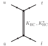
Figure 1: Feynman diagram generating a contribution to the $t\bar{t}$ asymmetry via a t-channel exchange of $K$ and $K^{*}$ resonances.

Our model is thus a realization of the effective t-channel models that have been discussed in the literature, but with both vector and (pseudo)scalar exchanges, rather than only one of these. The $K^{*}$ acts as the $Z^{\prime}$ in effective t-channel models Jung et al. (2010) and the $K$ as the (pseudo)scalar state Cui et al. (2011); Blum et al. (2011). At the LHC, the associated production of $K_{\rm HC}^{*}$ and $K_{\rm HC}$ in the $t\bar{t}j$ final state is also important for reducing the charge asymmetry $A_{\rm C}$, as stressed for $Z^{\prime}$ models in Drobnak et al. (2012). In order to avoid other constraints, e.g. bounds on top-jet resonance production at the LHC, the branching ratio of the decay $K_{\rm HC}^{*}\to q\bar{t}$ should be of order $25\%$. This is achieved naturally in our model since the $K_{\rm HC}^{*}$ decays dominantly into pairs of pseudoscalar mesons, in analogy with the decay $K^{*}\to K\pi$ in QCD.

Note that in order to have large $t\bar{t}$ asymmetry a relatively large Yukawa coupling between the HC and the SM fields is needed. For the considered values of the Yukawa couplings the two-loop renormalization-group equations (RGEs) suggest the existence of a strongly interacting UV fixed point. Under this assumption our theory can thus be extended to arbitrarily high scales in the UV.

The paper is organized as follows. In Section I we introduce our simple extension of the Standard Model, in Section II we discuss in detail the mass spectra and interactions of the resulting resonances, while Section III covers the LHC and Tevatron phenomenology, including the $t\bar{t}$ asymmetries. Section IV covers precision electroweak constraints, and perturbations of the Higgs properties. Future searches are covered in Section V, including a brief discussion of the lightest HC baryon and dark matter direct detection experiments. Our conclusions are collected in Section VI. Three appendices contain further details on translating information from QCD to the parameters of the effective HC interaction Lagrangians.

I The set-up.

QCD provides the prototype for a confining theory with a spectrum that contains flavorful vector mesons. Using QCD as a guide, we introduce an asymptotically free confining ${\rm SU}(N)_{\rm HC}$ hypercolor (HC) gauge group. The anomaly-free matter content consists of the SM and three copies of vectorlike hypercolor quarks ${\cal Q}_{Li},{\cal Q}_{Ri}$ ($i=1,2,3$) and a flavor-singlet hypercolor scalar ${\cal S}$, transforming as

$$\begin{split}{\cal Q}_{Li}&\sim(N,1,1,a)\,,\\ {\cal Q}_{Ri}&\sim(N,1,1,a)\,,\\ {\cal S}&\sim(\overline{N},3,1,b)\,,\end{split}$$ (1)

with respect to the gauge symmetry ${\rm SU}(N)_{\rm HC}\times{\rm SU}(3)_{\rm C}\times{\rm SU}(2)_{L}\times{\rm U}(1)_{Y}$. The hypercharge assignments satisfy $a+b=2/3$. The choice $a=0,b=2/3$ is phenomenologically favored, as we will see below, and will be used in the main part of the paper.

The most general renormalizable New Physics (NP) Lagrangian is given by

$$\begin{split}-{\cal L}_{\rm NP}=&\big{(}{\bf h}_{ij}\,\bar{u}_{Ri}\,{\cal Q}_{Lj}\,{\cal S}\,+\,{\rm h.c.}\big{)}\,+\,{\bf m_{\cal Q}}_{ij}\,\bar{{\cal Q}}_{i}\,{\cal Q}_{j}\\ &\,+\,\mu_{\cal S}^{2}\,{\rm Tr}({\cal S}^{\dagger}{\cal S})\,+\lambda_{1}{\rm Tr}({\cal S}^{\dagger}{\cal S})^{2}\\ &+\lambda_{2}{\rm Tr}({\cal S}^{\dagger}{\cal S}{\cal S}^{\dagger}{\cal S})+\lambda_{H}H^{\dagger}H\,{\rm Tr}({\cal S}^{\dagger}{\cal S})\,,\end{split}$$ (2)

plus the kinetic energy terms, where $H$ is the SM Higgs and $u_{Ri}$ the SM right-handed (RH) up quarks. The quartic interactions are not relevant for this work. However, we do require that the couplings $\lambda_{1,2},\lambda_{H}$ do not lead to a non-vanishing vacuum expectation value (vev) for ${\cal S}$. The total mass of the scalar ${\cal S}$ is $m_{\cal S}^{2}=\mu_{\cal S}^{2}+\lambda_{H}v^{2}/2$, where $v/\sqrt{2}$ is the SM Higgs vev. In the context of naturalness, we can imagine that the scalar ${\cal S}$ is actually composite, or we can invoke supersymmetry above $O(1~{}{\rm TeV})$ to protect its mass.

In the absence of Yukawa interactions and HC quark masses the theory respects the global symmetry group ${\rm G_{F}}={\rm U}(3)_{U_{R}}\times{\rm U}(3)_{D_{R}}\times{\rm U}(3)_{Q_{L}}$, like the SM. Under the ${\rm U}(3)_{U_{R}}$ symmetry both $({u_{R}}_{1},{u_{R}}_{2},{u_{R}}_{3})$ and $({\cal Q}_{1},{\cal Q}_{2},{\cal Q}_{3})$ transform as flavor triplets. In the SM the main sources of flavour breaking are the top and bottom Yukawa couplings that break $\rm G_{F}$ to its subgroup

$${\rm H_{F}}={\rm U}(2)_{U_{R}}\times{\rm U}(2)_{D_{R}}\times{\rm U}(2)_{Q_{L}}\times{\rm U}(1)_{3}\,.$$ (3)

Here we assume that the NP interactions also respect ${\rm H_{F}}$, i.e. the new Yukawa couplings and mass terms are of the form

$${\bf h}={\rm diag}(h_{1},h_{1},h_{3}),~{}{\bf m_{\cal Q}}={\rm diag}({m_{{\cal Q}}}_{1},{m_{{\cal Q}}}_{1},{m_{{\cal Q}}}_{3}).$$ (4)

The breaking of $\rm H_{F}$ in the SM is due to the light-quark Yukawa couplings and the CKM mixing angles, and is thus small. We will assume that this breaking continues to be small in our model. The approximate ${\rm U}(2)_{U_{R}}$ symmetry protects against dangerous flavor violation. We assume that its breaking is small, e.g., of MFV type. Thus, new contributions to $D_{0}$–$\overline{D_{0}}$ mixing as well as single and same-sign top production are negligible.

We stress the following: (i) the fact that the hypercolor matter only couples to the RH up quarks is due to the choice of representations. For example, had we chosen a hypercharge assignment such that $a+b=-1/3$ in Eq. (1), the hypercolor quarks ${\cal Q}_{i}$ would only couple to the RH SM down quarks. Alternatively, they could couple to the left-handed (LH) quarks if the ${\cal Q}_{i}$’s were ${\rm SU}(2)_{L}$ doublets. (ii) Our set-up is potentially compatible with generation of the quark mass and mixing hierarchies via spontaneous breaking of a horizontal non-abelian symmetry in the UV, e.g., ${\rm SU}(3)$, ${\rm SU}(2)$, or discrete non-abelian groups. In such a scenario the ${\rm U}(2)_{U_{R}}$ global symmetry of the hypercolor sector would be a consequence of the underlying horizontal symmetry, under which all of the quarks transform. (iii) The flavor structure of the resonance mass spectrum, to be discussed below, could provide a hint for the existence of such a fundamental horizontal symmetry in the UV (see also Ref. Grossman et al. (2007)).

HC Resonance	Mass	Decay Width
$\pi_{\rm HC}$	62 GeV	$4.0\cdot 10^{-7}\,m_{\pi}$
$K_{\rm HC}$	143 GeV	$5.5\cdot 10^{-7}\,m_{K}$
$\eta_{\rm HC}$	161 GeV	$1.3\cdot 10^{-7}\,m_{\eta}$
$\rho_{\rm HC}$	177 GeV	$0.059\,m_{\rho}$
$K^{*}_{\rm HC}$	211 GeV	$0.002\,m_{K^{*}}$
$V_{H}[\phi_{\rm HC}]$	242 GeV	$8.0\cdot 10^{-7}\,m_{V_{H}}$
$V_{L}[\omega_{\rm HC}]$	180 GeV	$0.001\,m_{V_{L}}$
$a_{1}^{\rm HC}$	273 GeV	$0.23\,m_{a_{1}}$
$K_{1}^{\rm HC}$	295 GeV	$0.057\,m_{K_{1}}$
$f_{1}^{\rm HC}$	280 GeV	$0.002\,m_{f_{1}}$
$f_{1}^{\prime}{}^{\rm HC}$	320 GeV	$3.2\cdot 10^{-5}\,m_{f_{1}^{\prime}}$

Table 1: The spectrum of the HC resonances for our benchmark.

II Hypercolor resonances and interactions

In order to make use of the available information on nonperturbative QCD dynamics, we take the HC gauge group to be ${\rm SU}(3)_{\rm HC}$. The HC condensates, resonance masses, and couplings are estimated via naive dimensional analysis (NDA), vector meson dominance (VMD), and/or scaling from QCD. The ${\cal Q}$ and ${\cal S}$ masses are taken to satisfy $m_{{\cal Q}_{i}}\ll\Lambda_{\chi}$ and $m_{\cal S}\gtrsim\Lambda_{\chi}$, where $\Lambda_{\chi}\sim 4\pi f_{\pi}$ is the HC chiral symmetry breaking scale (the motivation for this choice is given below, in Section II.3). We also introduce the scale $\Lambda_{\rm HC}\sim{\mathcal{O}}({\rm few})f_{\pi}$, which is the equivalent of $\Lambda_{\rm QCD}$ in QCD. The phenomenology that we are interested in is dominated by the lowest lying HC resonances. We thus keep the following resonances in the description

• the flavor octet of pseudo-Goldstone pseudoscalar resonances, $\pi^{a}_{\rm HC}$,

• the set of lowest lying vector, $\rho^{a}_{\rm HC}$, and axial vector, $a_{1,{\rm HC}}^{a}$, flavor nonet resonances.

In principle one could include additional HC resonances, e.g., the ${}^{1}P_{1}$ axial-vector multiplet (in QCD it contains the $b_{1}(1235)$ and $K_{1B}$). For simplicity, however, we ignore them in this work. Our notation is directly borrowed from QCD: $\pi_{\rm HC}$ is thus the equivalent of $\pi$ in QCD, etc. To shorten the notation we will often drop the HC subscript. For this reason in this paper the QCD states always carry a QCD subscript or superscript.

To illustrate the effect on $t\bar{t}$ production and other collider and low-energy observables we consider a benchmark in the parameter space. The benchmark resonance masses and decay widths are given in Table 1. The underlying UV parameters, as well as resonance couplings and decay constants are listed in Table 2. The determination of the resonance properties is described in detail below.

II.1 Pseudo-Nambu-Goldstone bosons

In the ${\rm U}(3)_{U_{R}}$ symmetric limit, the ${\cal Q}_{i}$ form equal condensates, $\langle\bar{\cal Q}{\cal Q}\rangle\neq 0$, which break the HC sector chiral symmetry to the diagonal subgroup, ${\rm SU}(3)_{L}\times{\rm SU}(3)_{R}\to{\rm SU}(3)_{V}$. This gives rise to a flavor octet of pseudo-Nambu-Goldstone bosons (pNGBs) $\pi^{a}_{\,\rm HC}$ ($a=1,\dots,8$). In NDA, $\Lambda_{\chi}\sim 4\pi f_{\pi}^{\,\rm HC}$ and

$$\langle\bar{\cal Q}{\cal Q}\rangle\sim 4\pi(f_{\pi}^{\,\rm HC})^{3},\,~{}~{}~{}~{}m^{2}_{\pi^{a}}\sim 8\pi f_{\pi}^{\,\rm HC}\,m_{\cal Q}\,,$$ (5)

where $f_{\pi}^{\,\rm HC}$ is the HC-pion decay constant,

$$\langle\pi^{a}|\bar{\cal Q}T^{a}\gamma_{\mu}\gamma_{5}{\cal Q}|0\rangle=-if^{\rm HC}_{\pi}p_{\mu}\,.$$ (6)

The flavor octet Gell-Mann matrices are normalized as ${\rm Tr}[T^{a}T^{b}]=\delta^{ab}/2$. For $\langle\bar{\cal Q}{\cal Q}\rangle$ we use the recent lattice determination of the QCD condensate McNeile et al. (2013), which gives $29.8(f_{\pi}^{\rm QCD})^{3}$, instead of the NDA estimate $4\pi(f_{\pi}^{\rm QCD})^{3}$ in Eq. (5) (in our convention $f_{\pi}^{\rm QCD}\simeq 92$ MeV). Similarly, for the pion mass we take $2\times 29.8$ instead of the factor $8\pi$ in Eq. (5). Requiring the vector resonances to have masses in the phenomenologically favored range of approximately $200$ GeV fixes $f_{\pi}^{\rm HC}\!\simeq\!20$ GeV, cf. Eq. (7) below. Thus, for $m_{\cal Q}\!\sim\!{\mathcal{O}}(10)$ GeV the masses of the pseudoscalars are $m_{\pi}^{\rm HC}\!\sim\!{\mathcal{O}}(100)$ GeV.

In our benchmark we take ${m_{{\cal Q}}}_{3}\!\sim\!f_{\pi}$ and ${m_{{\cal Q}}}_{1}\!\sim\!{m_{{\cal Q}}}_{3}/10$. The flavor symmetry breaking, $m_{{\cal Q}_{1}}\!\neq\!m_{{\cal Q}_{3}}$ leads to mass splitting between the $\pi\!\sim\![\bar{\cal Q}_{1,2}{\cal Q}_{1,2}]$, $K\!\sim\![\bar{\cal Q}_{1,2}{\cal Q}_{3}]$, and $\eta\!\sim\![\bar{\cal Q}_{1}{\cal Q}_{1}+\bar{\cal Q}_{2}{\cal Q}_{2}-2\bar{\cal Q}_{3}{\cal Q}_{3}]$, where the valence-quark content is given in square brackets. Details of the evaluation of their masses are given in Appendix A. The pseudoscalar mass spectrum also contains a heavier $\eta^{\prime}_{\rm HC}$ flavor singlet. The mass of the $\eta^{\prime}_{\rm HC}$ is $m_{\eta^{\prime}}\sim\Lambda_{\rm\chi}$, i.e., $m_{\eta^{\prime}}\!\sim{\mathcal{O}}(250)$ GeV. The $\eta_{\rm HC}^{\prime}$ has flavor diagonal couplings to the SM quarks. For the light quarks these are suppressed by the light quark masses. The $\eta_{\rm HC}^{\prime}$ thus has a negligible impact on $t\bar{t}$ and dijet phenomenology, as well as on the vector decay widths (due to its large mass). As such it can be omitted from our discussion. For simplicity we also neglect “$\,\eta-\eta^{\prime}\,$” mixing.

Param.	Value	Param.	Value	Param.	Value
$M_{\chi}$[GeV]	$171$	$g_{\rho}$	$4.88$	$f_{\pi}$	$20.4$ GeV
$m_{{\cal Q}_{1}}$[GeV]	$3.1$	$g_{\rho\pi\pi}$	$4.88$	$f_{\rho}$	$32.6$ GeV
$m_{{\cal Q}_{3}}$[GeV]	$30.5$	$g_{a_{1}}$	$6.73$	$f_{a_{1}}$	$37.1$ GeV
$m_{\cal S}$[GeV]	$520$	$g_{V_{o}}$	12.5	$f_{u^{\prime},c^{\prime}}$	$53.5$ GeV
$h_{1}$	$2.0$	$g_{V_{s}}$	$5.10$	$f_{t^{\prime}}$	$52.4$ GeV
$h_{3}$	$4.2$	$g_{A}$	$1.26$

Table 2: The UV parameters for the benchmark point (left two columns), the resulting HC resonance couplings (middle two columns), and the HC decay constants (last two columns).

II.2 Vectors and axial vectors

As in QCD, the $[\bar{\cal Q}{\cal Q}]$ bound states give rise to vector and axial-vector resonances that are flavor nonets. We denote the lowest lying states by $\rho_{\,\rm HC}^{a}$ and $a_{1\,\rm HC}^{a}$ ($a=1,\ldots,9$), respectively. Here, $\rho^{9}_{\rm HC}$ and $a_{1\,\rm HC}^{9}$ are the flavor-singlet states. Sometimes we will also use the generic notation of $V$ and $A$ for vector and axial-vector mesons.

We first discuss the properties of these resonances in the flavor-symmetric limit. The masses and decay constants can be estimated via the approximate scaling relations

$${f^{\,\rm HC}_{\pi}\over f^{\,\rm QCD}_{\pi}}\sim{f^{\,\rm HC}_{\rho\,(a_{1})}\over f^{\,\rm QCD}_{\rho\,(a_{1})}}\sim{m_{\rho\,(a_{1})}^{\,{HC}}\over m^{\,\rm QCD}_{\rho\,(a_{1})}}\,,$$ (7)

with $f_{\pi}^{\,\rm QCD}\simeq 92$ MeV. The $\rho_{\,\rm HC}^{a}$ and $a_{1\,\rm HC}^{a}$ decay constants are defined as

$$\langle\rho^{a}_{\rm HC}|\bar{\cal Q}\,T^{a}\,\gamma_{\mu}\,{\cal Q}|0\rangle =-if^{\rm HC}_{\rho}m^{\rm HC}_{\rho}\epsilon_{\mu}\,,$$ (8)

$$\langle a_{1\,\rm HC}^{a}|\bar{\cal Q}\,T^{a}\,\gamma_{\mu}\gamma_{5}\,{\cal Q}|0\rangle =-if^{\rm HC}_{a_{1}}m^{\rm HC}_{a_{1}}\epsilon_{\mu}\,,$$ (9)

where the flavor-singlet matrix $T^{9}\equiv I_{3\times 3}/\sqrt{6}$. In QCD, the $\rho$ decay constant is $f^{\rm QCD}_{\rho}\simeq 148$ MeV Beneke et al. (2007). The $a_{1}$ decay constant $f_{a_{1}}^{\rm QCD}$ is not well known. For example, a light-cone sum-rule determination yields $f_{a_{1}}^{\rm QCD}\simeq 168$ MeV Yang (2007). Isgur et al. Isgur et al. (1989) made a phenomenological determination from the $\tau^{+}\to\nu_{\tau}\,\pi^{+}\pi^{+}\pi^{-}$ branching ratio. Rescaling their result to the current PDG branching ratio Beringer et al. (2012) would yield $f_{a_{1}}\simeq 152$ MeV. (Note that the quoted values of the $\rho$ and $a_{1}$ decay constants have been reduced by a factor $1/\sqrt{2}$ to conform to our normalization for $f_{\pi}$.) As an example, taking the sum-rule value for $f_{a_{1}}^{\rm QCD}$, the scaling relations would imply

$$\frac{f^{\rm\,HC}_{\rho}}{m^{\rm\,HC}_{\rho}}\sim 0.19\,,\qquad\frac{f^{\rm\,HC}_{a_{1}}}{m^{\rm\,HC}_{a_{1}}}\sim 0.13\,,$$ (10)

in accord with Weinberg’s sum rules that require $f^{\rm\,HC}_{a_{1}}/m^{\rm\,HC}_{a_{1}}<f^{\rm\,HC}_{\rho}/m^{\rm\,HC}_{\rho}$. Eq. (7) also implies

$$\frac{m^{\rm\,HC}_{a_{1}}}{m^{\rm\,HC}_{\rho}}\sim 1.6\,.$$ (11)

Motivated by $A_{FB}^{t\bar{t}}$, we consider $m_{\rho}^{\rm\,HC}\sim 200$ GeV, corresponding to $f_{\pi}^{\rm\,HC}\sim 20$ GeV.

In the flavor symmetric limit, the flavor octet $\rho^{a}$ decays primarily to pairs of HC pions, with the decay width

$$\Gamma_{\rho\to\pi\pi}={g_{\rho\pi\pi}^{2}\over 32\pi}\,m_{\rho}\,\left(1-{4m_{\pi}^{2}\over m_{\rho}^{2}}\right)^{\frac{3}{2}}\,,$$ (12)

where $g_{\rho\pi\pi}$ is the $\rho\,\pi\,\pi$ coupling in

$${\cal L}_{\rho\pi\pi}=-g_{\rho\pi\pi}\,f_{abc}\,\rho_{\mu}^{a}\,\pi^{b}\partial^{\mu}\pi^{c}\,.$$ (13)

The VMD estimate

$$g_{\rho\pi\pi}\simeq m_{\rho}/f_{\rho}$$ (14)

agrees with the NDA estimate $g_{\rho\pi\pi}\sim{\mathcal{O}}(4\pi)$ within a factor of $\sim 2$. In QCD the VMD prediction is only $16\%$ smaller than the measured value. Based on the above we can expect $\Gamma_{\rho}/m_{\rho}\sim{\mathcal{O}}(10\%)$.

Flavor-symmetry breaking due to ${m_{{\cal Q}}}_{1}\neq{m_{{\cal Q}}}_{3}$ splits the $\rho\sim[\bar{\cal Q}_{1,2}{\cal Q}_{1,2}]$ and $K^{*}\sim[\bar{\cal Q}_{1,2}{\cal Q}_{3}]$ masses, as well as the corresponding $a_{1}$ and $K_{1}$ masses. In general, $g_{VPP}~{}$(=$g_{\rho\pi\pi}$ in the flavor-symmetric limit) now also depends on the vector and pseudoscalar flavors. Motivated by QCD, we allow for ${\mathcal{O}}(10\%)$ flavor breaking. The flavor breaking also leads to “${\omega}-\phi$” mixing as well as its axial-vector analog. We denote the deviation from ideal vector-meson mixing by the angle $\theta_{V}^{\rm id}$, so that the relation between the mass eigenstates $V_{L,H}$ and the ideally mixed states

$$|V_{12}\rangle={1\over\sqrt{2}}(|\bar{\cal Q}_{1}\,{\cal Q}_{1}\rangle+|\bar{\cal Q}_{2}\,{\cal Q}_{2}\rangle)\,,~{}~{}|V_{3}\rangle=|\bar{\cal Q}_{3}\,{\cal Q}_{3}\rangle\,,$$ (15)

is given by

$$\begin{pmatrix}|V_{L}\rangle\\ |V_{H}\rangle\end{pmatrix}=\begin{pmatrix}\cos\theta_{V}^{\rm id}&\sin\theta_{V}^{\rm id}\\ -\sin\theta_{V}^{\rm id}&\cos\theta_{V}^{\rm id}\end{pmatrix}\begin{pmatrix}|V_{12}\rangle\\ -|V_{3}\rangle\end{pmatrix}\,,$$ (16)

and similarly for the axial-vector mixing angle $\theta_{A}^{\rm id}$, with $V_{L,H}\to A_{L,H}$ and $V_{12,3}\to A_{12,3}$. Frequently, we will also employ QCD inspired notation for the mass eigenstates, i.e., $V_{L}=\omega_{\rm HC}$, $V_{H}=\phi_{\rm HC}$, and $A_{L}=f_{1}^{\rm HC}$, $A_{H}=f_{1}^{\prime}{}^{\rm HC}$. Since we do not include the ${}^{1}P_{1}$ resonances there is no equivalent of the $K_{1A}$-$K_{1B}$ mixing in our simplified formalism. In particular, we identify the $K_{1}^{\rm HC}$ in Table 1 with the equivalent of the $K_{1A}^{\rm QCD}$ in QCD.

Given $m_{{\cal Q}_{1}}$ and $m_{{\cal Q}_{3}}$, we determine the vector and axial-vector masses as well as the mixing angles $\theta_{V,A}^{\rm id}$ using the simplified quark-model treatment of Ref. Cheng and Shrock (2011). The HC hadronic parameters of this model are obtained by fitting to the QCD vector and axial-vector meson data, and then rescaling to the HC scale, $M_{\chi}$, as explained in detail in Appendix A. The HC scale is defined to be the $\rho$ mass in the chiral limit,

$$M_{\chi}\equiv\lim_{m_{{\cal Q}_{i}}\to 0}m_{\rho}.$$ (17)

In turn, the $\pi$, $\rho$ and $a_{1}$ decay constants are taken to be

$$f_{\pi} =\frac{M_{\chi}}{m_{\rho}^{\rm QCD}}f_{\pi}^{\rm QCD},$$ (18)

$$f_{\rho} =\frac{M_{\chi}}{m_{\rho}^{\rm QCD}}f_{\rho}^{\rm QCD},$$ (19)

$$f_{a_{1}} =\frac{M_{\chi}}{m_{a_{1}}^{\rm QCD}}f_{a_{1}}^{\rm QCD}$$ (20)

where the QCD decay constants that we use are $f_{\pi}^{\rm QCD}=92$ MeV, $f_{\rho}^{\rm QCD}=148$ MeV, and $f_{a_{1}}^{\rm QCD}=168$ MeV.

The $\rho_{\rm HC}$ resonances decay primarily to HC pion pairs, as in QCD, and subdominantly to light-quark pairs, cf. Table 5. The $K^{*}_{\rm HC}$ resonances decay primarily to $K_{\rm HC}+\pi_{\rm HC}$ pairs, as in QCD. Their subdominant decays to $t+$light quark pairs have a branching ratio of $\approx 30\%$, as explained in Section III.3. The fact that the $K^{*}_{\rm HC}\!\to\!t+$jet decays are subleading is phenomenologically favored and naturally achieved within our model, as already mentioned in the Introduction. In our benchmark both the $\omega_{\rm HC}$ and $\phi_{\rm HC}$ are kinematically forbidden to decay to on-shell $\bar{K}_{\rm HC}K_{\rm HC}$ pairs. Therefore, their dominant decays are to SM quarks with very narrow decay widths, cf. Table 1.

For the axial-vector meson decay widths we use the model of Ref. Roca et al. (2004), where a global ${\rm SU}(3)$ flavor symmetry is used for the matrix elements, but the phenomenologically more important effect of flavor-symmetry breaking in the phase space of the final states is kept. A hadronic parameter, $\tilde{F}_{\rm QCD}$, obtained from the fit to the $A\to PV$ decay widths in QCD Roca et al. (2004) is rescaled to $\tilde{F}_{\rm HC}$ in order to obtain the corresponding HC decay widths. See Appendix C and Eq. (101) for details. The HC $a_{1}$ state decays predominantly to $\rho_{\rm HC}\,\,\pi_{\rm HC}$ pairs, yielding a large decay width, $\Gamma_{a_{1}}\simeq 0.2m_{a_{1}}$. The branching ratio into light-quark pairs is small, ${\mathcal{O}}({\rm few~{}}\%)$. The HC $K_{1}$ resonance decays predominantly to $K_{\rm HC}^{*}\,\,\pi_{\rm HC}$ pairs, yielding $\Gamma_{K_{1}}\simeq 0.05m_{K_{1}}$. The $K_{1}\to u,c+t$ branching ratio is of ${\mathcal{O}}(5\%-10\%)$. In our benchmark the decays of the HC $f_{1}(=A_{L})$ and $f_{1}^{\prime}(=A_{H})$ to $K_{\rm HC}\,\,K^{*}_{\rm HC}$ pairs are kinematically forbidden. Therefore, they are very narrow with their dominant decays being to light-quark pairs.

II.3 Would-be composite quarks

In our benchmark, an on-shell HC scalar ${\cal S}$ decays to $u_{j}\bar{\cal Q}_{j}$ pairs well before HC hadronization can occur. In particular, the decay width of the heavy scalar ${\cal S}$ is

$$\Gamma_{\cal S}=\sum_{j}\Gamma_{{\cal S}\to u_{j}\bar{\cal Q}_{j}}\,,$$ (21)

where $j$ runs over $j=1,2,3$. The ${\cal S}\to u_{j}\bar{\cal Q}_{j}$ partial decay widths are given by

$$\begin{split}\Gamma_{{\cal S}\to u_{j}\bar{\cal Q}_{j}}\simeq{m_{\cal S}}\,\frac{|h_{j}|^{2}}{16\pi}\,,\end{split}$$ (22)

up to phase-space corrections which are at most of ${\mathcal{O}}(10\%)$. In our benchmark the Yukawa couplings are large ($h_{i}\sim 2-4$), leading to $\Gamma_{\cal S}\simeq 0.44\times m_{\cal S}\simeq 230$ GeV. The ${\cal S}$ therefore decays on a timescale that is much shorter than the HC hadronization timescale, which is governed by $\Lambda_{\rm HC}\!\sim\!{\mathcal{O}}({\rm few})f_{\pi}\!\sim\!{\mathcal{O}}(60{\rm~{}GeV})$. Consequently, there are no asymptotic bound states of two heavy HC scalars, ${\cal S}{\cal S}^{*}$, or of a HC scalar and a HC quark, ${\cal S}{\cal Q}_{i}$. (Had we taken the fundamental scalar to be much lighter, ${\cal S}{\cal S}^{*}$ bound states would form and clearly show up as resonances in the differential $t\bar{t}$ spectrum. We are thus led to a consider scalar mass $m_{\cal S}\gtrsim 0.5$ TeV.)

However, the picture changes for production of the elementary quarks $u_{Ri}$ via their Yukawa couplings to the composite operators ${\cal S}{\cal Q}_{i}$. The latter are also isosinglet QCD color triplets with hypercharge $2/3$. The SM right-handed up quarks can then be viewed as an admixture of the elementary $u_{Ri}$ and bound-state ${\cal S}{\cal Q}_{i}$ quark fields. Note that in this case the scalar ${\cal S}$ has virtuality $\sqrt{s}\!\equiv(p_{\cal S}^{2})^{1/2}$ lying well below $m_{\cal S}$. The ${\cal S}$ decay width becomes $s$ dependent, being obtained via the substitution $m_{\cal S}\to\sqrt{s}$ in Eq. (22), including the implicit phase-space factor. Thus its decay width is suppressed to levels $\mathrel{\hbox to0.0pt{\lower 4.0pt\hbox{\hskip 1.0pt$\sim$}\hss}\raise 1.0pt\hbox{$<$}}\Lambda_{\rm HC}$, and bound-state ${\cal S}{\cal Q}_{i}$ quark fields with virtuality much smaller than their would-be physical mass can form and mix into on-shell $u_{Ri}$.

To estimate the mixing or partial compositeness of the $u_{Ri}$, we assume that it is dominated by the lowest pole in the $T\{{\cal S}{\cal Q}_{i}(x),{\cal S}^{*}\bar{\cal Q}_{i}(0)\}$ two-point function, or equivalently, by the lowest pole in the ${\cal S}{\cal Q}_{i}\to{\cal S}{\cal Q}_{i}$ scattering $S$ matrix. In the calculation of the mixing we will treat the lowest pole as an asymptotic state. Formally, this corresponds to taking the limit $h_{i}\to 0$ in Eq. (22), making ${\cal S}$ stable.

The Yukawa couplings induce mass mixing between the would-be composite quarks and the elementary up quarks ($u_{i}=u,c,t$),

$$\sqrt{2}\,h_{i}f_{u_{i}^{\prime}}\,{\bar{u}}_{Ri}\,{u^{\prime}}_{Li}\,,$$ (23)

where the would-be composite quark decay constants $f_{u_{i}^{\prime}}$ are defined as

$$\langle u_{i}^{\prime}|\bar{\cal Q}_{i}\,{\cal S}^{*}|0\rangle=\sqrt{2}f_{u_{i}^{\prime}}\,{\bar{u}}_{i}^{\prime}\,.$$ (24)

Here the ${\bar{u}}_{i}^{\prime}$ are the Dirac spinors.

Since $m_{{\cal Q}}\ll m_{\cal S}$ the would-be composite HC quarks correspond to bound states of a heavy–light quark system. More precisely, in our benchmarks $m_{\cal S}$ is $\sim 2\Lambda_{\rm HC}$. Comparing to QCD this corresponds to a heavy–light quark system with a heavy quark mass lying somewhere between the charm and bottom quark mass. To estimate the $f_{u^{\prime}_{i}}$ decay constants we therefore interpolate between the known light–light and heavy–light vector-meson decay constants in QCD, and rescale to the case of HC – see Appendix B, Eq. (89) in particular, for details.

For the purpose of this discussion we can take the ordinary $3\times 3$ up-quark mass matrix to be flavor diagonal, neglecting the small misalignment between the weak and up-quark mass bases in the SM. For each generation the mixing between the SM and would-be HC quarks is then described by $2\times 2$ matrices

$$M_{RL}^{i}=\left(\begin{array}[]{ll}m_{u_{i}}{}&\sqrt{2}h_{i}f_{u_{i}^{\prime}}\\ 0{}&~{}M_{u_{i}^{\prime}}\end{array}\right),~{}~{}i=1,2,3.$$ (25)

Here $m_{u_{i}}$ is the ordinary ${\rm SU}(2)_{L}$ breaking quark mass, and $M_{u_{i}^{\prime}}\simeq m_{{\cal Q}_{i}}+m_{u_{i}}+\Lambda_{\rm HC}$ is the mass term for the would-be composite quark (see Eq. (84)). The mixing term follows from Eq. (23).

Diagonalization of Eq. (25) yields the mass eigenstates

$$|u_{Ri}\rangle^{\rm phys} =\cos\theta_{Ri}\,|u_{Ri}\rangle-\sin\theta_{Ri}\,|u^{\prime}_{Ri}\rangle\,,$$ (26)

$$|u^{\prime}_{Ri}\rangle^{\rm phys} =\sin\theta_{Ri}\,|u_{Ri}\rangle+\cos\theta_{Ri}\,|u^{\prime}_{Ri}\rangle\,,$$ (27)

and similarly for the LH mass eigenstates with the replacement $R\to L$. The ordinary $u,c$, and $t$ quarks are identified with $u_{1}^{\rm phys}$, $u_{2}^{\rm phys}$, and $u_{3}^{\rm phys}$, respectively. Taking $h_{i}f_{u^{\prime}_{i}}$ significantly smaller than $M_{u^{\prime}_{i}}$ yields

$$\sin\theta_{Ri}\sim\sqrt{2}h_{i}{f_{u_{i}^{\prime}}\over M_{u_{i}^{\prime}}}\,,~{}~{}~{}\sin\theta_{Li}\sim\sqrt{2}h_{i}{f_{u_{i}^{\prime}}m_{u_{i}}\over M^{2}_{u_{i}^{\prime}}}\,.$$ (28)

The RH mixings are substantially larger than the LH ones, which are suppressed by the $M_{u_{i}^{\prime}}$. Specifically, for our benchmark we find

$$\sin\theta_{R1}=\sin\theta_{R2}=0.22\,, \sin\theta_{R3}=0.43\,,$$ (29)

$$\sin\theta_{L1}=\sin\theta_{L2}\approx 0\,, \sin\theta_{L3}=0.10\,.$$ (30)

The couplings of the vector mesons to the would-be composite quarks are given by

$${\cal L}=g_{\rho}(\bar{u}^{\prime}T^{a}\gamma^{\mu}u^{\prime})\rho^{a}_{\mu}+g_{a_{1}}(\bar{u}^{\prime}T^{a}\gamma^{\mu}\gamma_{5}u^{\prime}){a_{1}}^{a}_{\mu}\,+\cdots\,.$$ (31)

Here, the $u^{\prime}$ appear in the interaction basis of Eqs. (23)–(25) and, for simplicity, we have taken flavor-symmetric couplings. The ellipses denote higher-derivative operators. In NDA, both $g_{\rho}$ and $g_{a_{1}}$ are ${\mathcal{O}}(4\pi)$, while the VMD estimates are (see Appendix B)

$$g_{\rho}\simeq{m_{\rho}\over f_{\rho}}\,,~{}~{}~{}g_{a_{1}}\simeq{m_{a_{1}}\over f_{a_{1}}}\,,$$ (32)

so that $g_{\rho}\simeq g_{\rho\pi\pi}$. In the numerics below we will take them to be equal.

Couplings of the vector mesons to the SM quarks are induced then via the quark mixing in Eq. (26). In the quark-mass basis these couplings are given by

$$~{}\begin{split}{\cal L}=&\lambda^{R}_{ij}\,\bar{u}_{Ri}\gamma^{\mu}T_{ij}^{a}\rho^{a}_{\mu}u_{Rj}+(R\to L)+\cdots\,,\end{split}$$ (33)

where

$$\begin{split}\lambda^{R}_{ij}=&~{}g_{\rho}\sin\theta_{Ri}\sin\theta_{Rj}\,,\end{split}$$ (34)

and the ellipses denote terms involving the would-be composite quarks.

The LH quark couplings $\lambda_{i}^{L}$ are obtained by substituting $R\to L$ in Eqs. (33)–(34). The axial-vector meson couplings to quarks follow by substituting $\gamma^{\mu}\to\gamma^{\mu}\gamma_{5}$ and $g_{\rho}\to g_{a_{1}}$. The $K^{*}ut$ coupling $\lambda_{113}^{R}$ and the corresponding $K_{1}ut$ coupling are phenomenologically important for NP contributions to $t\bar{t}$ production from t-channel HC resonance exchanges. On the other hand, the s-channel contributions from $\phi/\omega$ as well as $f_{1}/f_{1}^{\prime}$ exchanges are suppressed by the small $\theta_{V,A}^{\rm id}$ mixing angles. The above couplings also govern the partial decay widths of the vector and axial-vector resonances to quark pairs.

Similarly, the interactions of the HC pions with the SM quarks follow from their couplings to the would-be composite quarks,

$${\cal L}=\frac{g_{A}}{f_{\pi}}\Big{(}\bar{u}^{\prime}_{Ri}\,T^{a}_{ij}\,\cancel{\partial}\pi^{a}u^{\prime}_{Rj}-\bar{u}^{\prime}_{Li}\,T^{a}_{ij}\,\cancel{\partial}\pi^{a}u^{\prime}_{Lj}\Big{)}\,+\cdots,$$ (35)

where the ellipses again denote higher-derivative operators. In NDA $g_{A}\sim{\mathcal{O}}(1)$, consistent with the QCD nucleon-pion axial coupling $g_{A}^{\rm QCD}\simeq 1.26$. Ignoring the spin structure, as warranted in the heavy-scalar limit, one can also compare $g_{A}$ with the QCD $B^{*}B\pi$, and $D^{*}D\pi$ couplings, which are also ${\mathcal{O}}(1)$ (i.e., $\hat{g}\sim 0.6-0.7$ Abada et al. (2004); Ohki et al. (2008); El-Bennich et al. (2011)).

Changing to the physical quark basis, the Lagrangian is given by

$$\begin{split}{\cal L}=\frac{g_{A}}{f_{\pi}}&\sin\theta_{Ri}\sin\theta_{Rj}\,\bar{u}_{Ri}\,T^{a}_{ij}\,\cancel{\partial}\pi^{a}u_{Rj}-\big{(}R\to L\big{)}\,,\end{split}$$ (36)

where we do not show the terms that involve would-be HC quarks. Integrating by parts and using the Dirac equation, Eq. (36) is equivalent on the quark mass shell to

$$\begin{split}{\cal L}\simeq&\frac{ig_{A}}{f_{\pi}}\sin\theta_{Ri}\sin\theta_{Rj}m_{u_{j}}\,\bar{u}_{Ri}\,T_{ij}^{a}\pi^{a}u_{Lj}\\ &+\rm h.c.-\big{(}R\to L\big{)}\,.\end{split}$$ (37)

We see that the only significant contribution is proportional to $m_{t}$. Thus, production of $t\bar{t}$ pairs receives important contributions from t-channel $K$ exchange. In contrast, s-channel contributions are suppressed by the light-quark masses.

The couplings in Eq. (37) are also responsible for pion decays to quark pairs, e.g. $\pi\to 2j$, $K\to jt^{*}$. The $\pi^{a}$ decay widths are given by

$$\begin{split}&\frac{\Gamma_{\pi^{a}\to\bar{u}_{i}u_{j}}}{m_{\pi^{a}}}=\frac{g_{A}^{2}N_{c}}{16\pi}\frac{\big{(}m_{u_{j}}^{2}+m_{u_{i}}^{2}\big{)}}{f_{\pi}^{2}}T^{a}_{ij}T^{a}_{ji}\sin\theta_{Ri}^{2}\sin\theta_{Rj}^{2},\end{split}$$ (38)

where $a=1,2,3$, and we do not write down terms further supressed by the light-quark masses. While the decay widths are narrow due to light-quark mass suppression, they do not lead to displaced vertices since they correspond to decay lengths of tens of nanometers.

III Tevatron and LHC Phenomenology

Next, we assess the effect of the new HC sector on the $t\bar{t}$ production cross sections and asymmetries at the Tevatron and the LHC. The relevant measurements and the corresponding SM predictions are collected in Table 3 and Table 4. As an example we take the benchmark set of parameters introduced in the previous section. It has been chosen to demonstrate that our model can easily yield anomalously large $A_{\rm FB}^{t\bar{t}}$ asymmetries, while satisfying the remaining $t\bar{t}$ constraints. We also show that the benchmark passes the Tevatron and LHC dijet tests that often invalidate models addressing the Tevatron $A_{\rm FB}^{t\bar{t}}$ anomalies. Cross sections for the production of new resonances that are present in our model are evaluated, and the most promising signals are identified. In Section IV we will discuss another class of constraints, namely electroweak precision tests, including atomic-parity violation.

III.1 The top-antitop asymmetries: experimental review

The CDF and DØ  experiments at the Tevatron have measured various partonic level asymmetries in $p\bar{p}\to t\bar{t}$. One of these is the inclusive asymmetry,

$$A_{\rm FB}\equiv\frac{N(\Delta y>0)-N(\Delta y<0)}{N(\Delta y>0)+N(\Delta y<0)}\,,$$ (39)

where $\Delta y=y_{t}-y_{\bar{t}}$ is the difference between the $t$ and $\bar{t}$ rapidities, taking the forward direction to be that of the proton. The SM prediction for the inclusive asymmetry is

$$A_{\rm FB}^{\rm SM}=0.088\pm 0.006\,.$$ (40)

This result uses NLO cross-section differences, including leading EW corrections, in the numerator Kuhn and Rodrigo (1998, 1999, 2012); Ahrens et al. (2011); Manohar and Trott (2012); Hollik and Pagani (2011); Bernreuther and Si (2012); and LO cross sections in the denominator. Note that use of the NLO cross sections in the denominator would reduce the predicted asymmetry by ${\mathcal{O}}(30\%)$. The NLO PDF set CTEQ6.6m Nadolsky et al. (2008) is used throughout. The error in Eq. (40) is the pure scale uncertainty for $\mu\in[m_{t}/2,2m_{t}]$.

The CDF Aaltonen et al. (2013a) measurement of $A_{\rm FB}$ is larger than the SM prediction, as was the 2011 DØ  measurement. A new DØ  measurement Abazov et al. (2014), extended to include a 3-jet sample in $t\bar{t}$ production, is significantly lower and supersedes the previous one. Naively averaging with CDF yields

$$A_{\rm FB}^{\rm inc}=0.124\pm 0.025\,.$$ (41)

Observable	Value	Ref.
$A_{\rm FB}^{\rm low,\,CDF}$	$0.084\pm 0.055$	Aaltonen et al. (2013a)
$A_{\rm FB}^{\rm high,\,CDF}$	$0.295\pm 0.067$	Aaltonen et al. (2013a)
$A_{\rm FB}^{\rm inc,\,CDF}$	$0.164\pm 0.047$	Aaltonen et al. (2013a)
$A_{\rm FB}^{\rm inc,\,{\rm D\O}}$	$0.106\pm 0.030$	Abazov et al. (2014)
$A_{\rm FB}^{\rm inc,\,average}$	$0.124\pm 0.025$
$A_{\rm C}^{\rm inc,\,ATLAS,\,semileptonic}$	$0.006\pm 0.010$	ATL (2013a)
$A_{\rm C}^{\rm inc,\,ATLAS,\,dileptons}$	$0.057\pm 0.028$	ATLAS:2012sla (1204260)
$A_{\rm C}^{\rm inc,\,CMS,\,semileptonic}$	$0.004\pm 0.015$	Chatrchyan et al. (2012a)
$A_{\rm C}^{\rm inc,\,CMS,\,dileptons}$	$-0.010\pm 0.019$	Chatrchyan et al. (2014a)
$A_{\rm C}^{\rm inc,7TeV,average}$	$0.007\pm 0.008$
$A_{\rm C}^{\rm inc,CMS,8TeV}$	$0.005\pm 0.009$	CMS (2013)
$\sigma_{\rm inc}^{\rm CDF+D\O}$	$(7.60\pm 0.41){\rm\,pb}$	Aaltonen et al. (2013b)
$\sigma_{\rm inc}^{\rm ATLAS}$ (7 TeV)	$(177\pm 11){\rm\,pb}$	ATL (2012a)
$\sigma_{\rm inc}^{\rm ATLAS}$ (8 TeV)	$(237.7\pm 11.3){\rm\,pb}$	ATL (2013b)
$\sigma_{\rm inc}^{\rm CMS}$ (7 TeV)	$(165.8\pm 13.3){\rm\,pb}$	CMS (2011)
$\sigma_{\rm inc}^{\rm CMS}$ (8 TeV)	$(239\pm 13){\rm\,pb}$	Chatrchyan et al. (2014b)

Table 3: Experimental input for $t\bar{t}$ production cross section and asymmetries. All errors have been added in quadrature.

Observable	Value	Ref.
$A_{\rm FB}^{\text{low, SM}}$	$0.062\pm 0.003$	Bernreuther and Si (2012)
$A_{\rm FB}^{\text{high, SM}}$	$0.129\pm 0.006$	Bernreuther and Si (2012)
$A_{\rm FB}^{\text{inc, SM}}$	$0.088\pm 0.006$	Bernreuther and Si (2012)
$A_{\rm C}^{\rm SM}$ (7 TeV)	$0.0123\pm 0.0005$	Bernreuther and Si (2012)
$A_{\rm C}^{\rm SM}$ (8 TeV)	$0.0111\pm 0.0004$	Bernreuther and Si (2012)
$\sigma_{\rm inc}^{\rm TEV,\,NNLO}$	$(7.395\pm 0.544){\rm\,pb}$	Czakon et al. (2013)
$\sigma_{\rm inc}^{\rm LHC,\,NNLO}$ (7 TeV)	$(172.5\pm 15.0){\rm\,pb}$	Czakon et al. (2013)
$\sigma_{\rm inc}^{\rm LHC,\,NNLO}$ (8 TeV)	$\big{(}246.3^{+19.8}_{-20.5}\big{)}{\rm\,pb}$	Czakon et al. (2013)

Table 4: SM predictions for $t\bar{t}$ production cross section and asymmetries.

Interestingly, CDF observes a significant rise in $A_{\rm FB}$ with the invariant mass of the $t\bar{t}$ pair. Quoting just their two-bin result as an example, they report

$$A_{\rm FB}^{\rm low}=0.084\pm 0.046\pm 0.030\,,$$ (42)

for $m_{t\bar{t}}\leq 450$ GeV and

$$A_{\rm FB}^{\rm high}=0.295\pm 0.058\pm 0.033\,,$$ (43)

for $m_{t\bar{t}}\geq 450$ GeV, which should to be compared to the SM predictions Bernreuther and Si (2012)

$$A_{\rm FB}^{\rm low,SM}=0.062\pm 0.003\,,$$ (44)

and

$$A_{\rm FB}^{\rm high,SM}=0.129\pm 0.006\,.$$ (45)

The CDF and DØ  collaborations have also presented results with finer, albeit different, binning in $m_{t\bar{t}}$ Abazov et al. (2014); Aaltonen et al. (2013a). The two sets of measurements are consistent with each other, with the exception of the largest bin, $m_{t\bar{t}}>650$ GeV, for which DØ  obtains a negative central value with an error that is 68% larger than CDF’s. In the $m_{t\bar{t}}\in[550,650]$ bin, the DØ  and CDF central values are very close but the DØ  error is 60% larger. The CDF fitted slope for $A_{\rm FB}$ vs $m_{t\bar{t}}$ is $1.8\sigma$ larger than DØ’s, and $2.4\sigma$ larger than the NLO SM prediction. Both collaborations have also measured $A_{\rm FB}$ vs. the rapidity difference $\Delta y$, again with different binning. The CDF fitted slope is $1.3\sigma$ larger than DØ’s, and $2.4\sigma$ larger than the NLO SM prediction.

At the LHC, the initial state is symmetric, thus there is no fixed forward or backward direction with respect to which an asymmetry can be defined. Instead, the observable that is related to $A_{\rm FB}$ is the charge asymmetry,

$$A_{\rm C}=\frac{N(\Delta|y|>0)-N(\Delta|y|<0)}{N(\Delta|y|>0)+N(\Delta|y|<0)}\,,$$ (46)

where $\Delta|y|=|y_{t}|-|y_{\bar{t}}|$ is the difference between the absolute values of the top and antitop rapidities. At $7$ TeV both ATLAS and CMS have measured the charge asymmetry in the semileptonic and dilepton decay channels, albeit with appreciable experimental uncertainties (see Table 3). Naively averaging the four measurements yields

$$A_{\rm C}^{\rm EXP} =0.007\pm 0.008\,,$$ (47)

consistent with the SM prediction Bernreuther and Si (2012)

$$A_{\rm C}^{\rm SM} =0.0123\pm 0.0005\,.$$ (48)

(Only averaging the two semileptonic measurements yields $A_{\rm C}^{\rm exp}=0.005\pm 0.009$.) Again, the SM prediction has been obtained with the LO cross section in the denominator. An 8 TeV measurement of $A_{\rm C}$ was recently presented by CMS CMS (2013),

$$A_{\rm C}=0.005\pm 0.009\,,$$ (49)

which is also consistent with the SM prediction Bernreuther and Si (2012)

$$A_{\rm C}=0.0111\pm 0.0004\,.$$ (50)

Whether or not the experimental situation at the Tevatron points to an anomalously large forward-backward asymmetry or is due to statistical fluctuations, our philosophy will be to show that in our model large enhancements of $A_{\rm FB}$ can be consistent with all other constraints, thus highlighting the stealth nature of the new strong interactions.

III.2 Choosing a benchmark

We calculate the asymmetries in our NP model using the procedure outlined in Ref. Drobnak et al. (2012), and employed in Ref. Bernreuther and Si (2012) for the SM predictions given above. In the numerator we take the SM at NLO (QCD + EW), and work with LO cross sections in the denominators. The contributions from NP (including NP–SM interference) in both the numerator and denominator are always evaluated at LO. All LO cross sections are automatically evaluated in Madgraph Alwall et al. (2011) using the NLO PDF-set CTEQ6m with a fixed renormalisation and $\alpha_{s}$ scale. For the benchmark presented here we fix the renormalisation scale to $\mu=2m_{t}$.

To obtain the Tevatron and LHC total $t\bar{t}$-production cross sections and differential $d\sigma/dm_{t\bar{t}}$ spectra we use the NNLO CTEQ10 predictions Czakon et al. (2013) at $\mu=m_{t}$ for the total SM cross sections, with their reported errors (see Table 4 ); and aMC@NLO for the differential SM spectra, evaluated at $\mu=m_{t}$, with the errors reflecting the scale and pdf uncertainties. The NP contributions to the total and differential spectra are evaluated at LO for a fixed scale choice, $\mu=2m_{t}$, as in the asymmetries.

Two of the explanations that have been proposed for the potential Tevatron $A_{\rm FB}^{t\bar{t}}$ anomalies are t-channel exchange of light vectors, e.g., $W^{\prime}$, $Z^{\prime}$ Jung et al. (2010), or of light scalars Blum et al. (2011). In both cases the exchanged particle’s mass is optimally a few hundred GeV or less. The models can yield a large $A_{\rm FB}^{t\bar{t}}$ that, particularly in the case of vector exchange, increases appreciably with $m_{t\bar{t}}$. Moreover, both proposals have been shown to simultaneously lead to good agreement with the $d\sigma/dm_{t\bar{t}}$ spectra (for the t-channel exchanges, correcting for the CDF acceptance at large pseudorapidity is crucial Gresham et al. (2011); Jung et al. (2011); Grinstein et al. (2011b)).

Our model provides a concrete renormalizable example that combines the two proposals. The role of the $Z^{\prime}$ is played by the HC $K^{*}$ and, to a lesser extent, by the $K_{\rm 1}$. The t-channel scalar corresponds to the HC $K$. Note that for high $m_{t\bar{t}}$ there are also perturbative contributions coupling to the RH up-type quarks from intermediate $S-{\cal Q}$ box graphs, which scale as

$${h_{1}^{2}h_{3}^{2}\over 16\pi^{2}}{1\over m_{t\bar{t}}^{2}}\sim{1\over 2m_{t\bar{t}}^{2}}\,.$$ (51)

However, we find that their effects are subleading and do not consider them further.

At the LHC, important constraints come from $\sigma_{t\bar{t}}$ and $A_{\rm C}$. An increase in $A_{\rm FB}^{t\bar{t}}$ via t-channel exchange is typically correlated with an increase in $A_{\rm C}$ beyond its measured value. However, associated light-mediator production, e.g. $gq\to t+(Z^{\prime}\to\bar{t}q)$, has been shown to reduce $A_{\rm C}$ Drobnak et al. (2012). Associated light-mediator production also contributes to the total LHC cross section, $\sigma_{t\bar{t}}$. The resulting constraint, as well as the ATLAS and CMS bounds from $t$+jet resonance searches, are evaded if the light mediator has other open decay channels, thus suppressing the $Z^{\prime}\to\bar{t}q$ branching ratio. In our model a new dominant decay channel is naturally present. In particular, the strong interaction decay $K^{*}\to K\pi$ can lead to ${\rm Br}(K^{*}\to\bar{t}j)\sim{\mathcal{O}}(30\%)$. This would still allow for a significant reduction of $A_{\rm C}$. Note that on-shell $K\to t+j$ decays are kinematically forbidden, so that the above constraints do not apply.

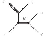
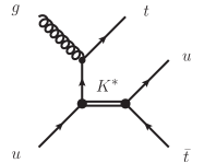
Figure 2: Feynman diagrams for the associated production of a $K$ and $K^{*}$, respectively. The $\bar{t}$ resulting from the $K$ decay is off-shell.

Previous studies, as outlined above, thus motivate us to search for benchmarks with relatively light $K^{*}$ and $K$, with masses of $\sim 200$ GeV. Moreover, a $\rho$ mass in this range is also favored by the recent CDF bounds on pair production of dijets Aaltonen et al. (2013c). For $\rho\to\pi\pi\to jj\,jj$ with $m_{\rho}\lesssim 200$ GeV and $m_{\pi}\sim$ 70 GeV the bounds weaken significantly and, in fact, lie above the expected limits.

In order to obtain a viable set of parameters for our model that i) yields substantially enhanced $A_{\rm FB}^{\rm t\bar{t}}$ at the Tevatron and ii) yields agreement with all other constraints, we employ a rough $\chi^{2}$-minimization procedure containing a subset of available measurements. Minimizing the $\chi^{2}$ with respect to a large number of variables is algorithmically difficult. We use the COBYLA method Powell (1998), which allows us to apply constraints on the minimization procedure.

The $\chi^{2}$ contains the experimental values of the inclusive $A_{\rm FB}^{t\bar{t}}$ and $A_{\rm C}$ ($7$ TeV), the total $t\bar{t}$ cross sections at the Tevatron and the LHC ($7$ TeV), and the highest bins of the differential cross sections at ATLAS ($7$ TeV), and CMS ($8$ TeV). The UV inputs are $h_{1},h_{3},m_{{\cal Q}_{1}},m_{{\cal Q}_{3}}$, $m_{\cal S}$, and the HC scale $M_{\chi}$ defined in Eq. (17). Through dimensional transmutation, the latter is equivalent to the choice of HC strong coupling constant, $\alpha_{\rm HC}$, in the UV. The UV parameters fix the pseudoscalar masses via the quadratic terms in the HC chiral Lagrangian, and the vector and axial-vector masses via the naive quark model described in Appendix A. The would-be composite quark masses in the interaction basis are given by Eq. (84). The decay constants $f_{\pi},f_{\rho}$, and $f_{a_{1}}$ (for simplicity taken to be universal for all members of the corresponding flavor octets), are given in Eqs. (18)–(20). The would-be composite quark decay constants $f_{u^{\prime}_{i}}$ are allowed to vary within $30\%$ of the interpolation given in Eq. (89).

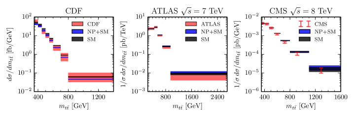
Figure 3: The differential cross sections, $d\sigma/dm_{t\bar{t}}$, at Tevatron (first panel) and at the LHC ($7$ TeV ATLAS in the second and $8$ TeV CMS in the third panel), SM prediction in black, the NP benchmark predictions in blue and measurements by CDF given by red bands.

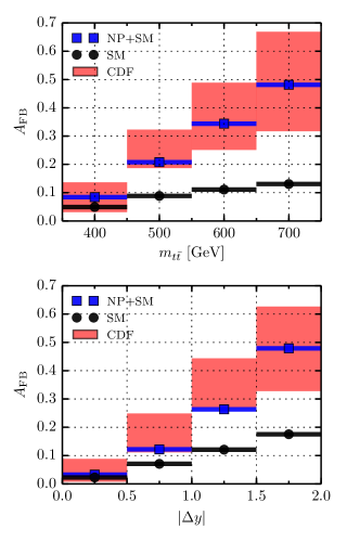
Figure 4: Differential $A_{\rm FB}$ asymmetries at the Tevatron as a function of $m_{t\bar{t}}$ (top) and $\Delta y$ (bottom) with the SM prediction in black, the NP benchmark predictions in blue and the measurements by CDF given by red bands.

We must also choose values for the couplings of the HC resonances to the would-be composite quarks, i.e. $g_{\rho}$, $g_{a_{1}}$, and $g_{A}$. We allow $g_{\rho}$ and $g_{a_{1}}$ to lie within roughly $30\%$ of the values obtained from Eq. (32), and we take $g_{A}=1.26$, identifying it with the representative QCD nucleon-pion axial coupling. The vector-pion coupling $g_{\rho\pi\pi}$ is taken to be equal to $g_{\rho}$. The decay widths of the vector meson multiplet, $\rho,K^{*},...$, are determined via Eqs. (90)–(92). The axial decay widths are determined using the model of Roca et al. (2004), see Eqs. (97)–(101), with the parameter $\tilde{F}_{\rm HC}$ fixed to the value obtained from Eq. (101). The pseudoscalar decay widths (LABEL:eq:pi:dec) are small and do not enter into our analysis.

HC Resonance	channel	Br(%)
$\rho_{\rm HC}$	$\pi\pi$	$98.2$
	$\bar{u}c,\bar{c}u,\bar{u}u+\bar{c}c$	$1.8$
$K^{*}_{\rm HC}$	$K\pi$	$68$
	$\bar{u}t,\bar{t}u,\bar{c}t,\bar{t}c$	$32$
$V_{H}[\phi_{\rm HC}]$	$\bar{u}u+\bar{c}c$	$100$
$V_{L}[\omega_{\rm HC}]$	$\bar{u}u+\bar{c}c$	$100$

Table 5: Table of the dominant branching ratios of HC vector resonances and their decays into SM quarks.

The UV or fundamental parameters for our illustrative benchmark are listed in Table 2, together with the resonance couplings and decay constants. The resonance masses and decay widths are given in Table 1. Realization of the phenomenologically favored range ${\rm Br}(K^{*}\to\bar{t}j)\sim 30\%$ arises via phase-space suppression of the dominant $K^{*}\to K\pi$ decay mode, see Table 5. Since $m_{K}^{*}\simeq m_{K}+m_{\pi}$ the phase-space factor is small, of $O(10^{-2})$ in our benchmark. The tuning associated with the phase-space suppression is actually quite moderate, given that the approximate equality of $m_{K}^{*}$ and $m_{K}+m_{\pi}$ changes relatively slowly as the HC quark masses $m_{{\cal Q}_{3}}$, $m_{{\cal Q}_{1}}$ are varied. For instance, the Barbieri-Giudice measure of fine tuning for the phase-space suppression factor, corresponding to variation of the HC quark masses around the benchmark point and using the naive quark model for the vector masses, is $\approx 8$. It is comparable to the tuning associated with the coincidence of $m_{\phi}$ and $2m_{K}$ in QCD.

Before moving to the resulting phenomenology, we comment on the large benchmark Yukawa couplings $h_{3}=4.2$, $h_{1}=2.0$. This is driven by two factors: a sizable product of couplings $h_{1}h_{3}$ is required in order to obtain a large t-channel enhancement of the forward-backward asymmetry, e.g. $A_{\rm FB}>0.15$; and $h_{1}$ is bounded from above by dijet constraints, most notably the CDF bounds on dijet pair production, see below. A moderate decrease in $h_{3}$ is possible if the non-perturbative couplings $g_{\rho}$ or $g_{A}$ of the vector or pseudoscalar mesons to the would-be composite quarks are moderately increased, or if $h_{1}$ is maximized consistently with dijet phenomenology. Nevertheless, a large $h_{3}$ is required, e.g., $h_{3}>3$.

The values of the Yukawa couplings $h_{1}$, $h_{3}$ in Table 2 correspond to a renormalization scale which can be approximately identified with $m_{\cal S}$. A large $h_{3}$ at this scale prompts us to ask if our theory is sensible at higher energies. For example, whether we encounter a Landau pole as we evolve $h_{1}$, $h_{3}$ and the HC gauge coupling $g_{\rm HC}$ upwards in energy. To answer this, we fix the values of $h_{1}(m_{\cal S})$, $h_{3}(m_{\cal S})$ to those given in Table 2. We also take $g_{\rm HC}(m_{\cal S})=1.9$, the value we would obtain for the QCD coupling $g_{s}$ at scale $\mu=m_{\cal S}\,f_{\pi}/f_{\pi}^{\rm HC}$ by running upwards with 3 flavors rather than 4 (given the 3 HC quark flavors) from its usual two-loop $\overline{\rm MS}$ value at $\mu=1$ GeV. The one-loop RGEs yield a Landau pole at $\mu\approx 1.6$ TeV. However, moving to two-loop RGEs using the general results from Ref. Luo et al. (2003) we find that $h_{3}$ reaches an approximate attractive UV fixed point at $\mu=O(10)$ TeV, given by $h_{3}^{*}=16\,\pi/\sqrt{37}\approx 8.3$, while $h_{1}$ and $g_{\rm TC}$ are asymptotically free. For lower values of $h_{3}(m_{\cal S})>3$ (see above), with $h_{3}(m_{\cal S})>h_{1}(m_{\cal S})$, the one-loop Landau pole and the two-loop UV fixed point for $h_{3}$ are, respectively, reached at scales that are a few times larger. Clearly, given the large value of $h_{3}^{*}$ obtained at two-loops, the question of whether a true UV fixed-point exists or not can only be settled using nonperturbative methods.

Consistency of our model requires that there are no QCD and HC breaking condensates, $\langle\bar{u}_{R3}\,{\cal Q}_{L3}\rangle\neq 0$ and $\langle{\cal S}\rangle\neq 0$, which could potentially be triggered by a large value of $h_{3}$. An estimate of the critical Yukawa coupling above which condensates form can be obtained using the Schwinger-Dyson equation at one-loop in the rainbow or ladder approximation in the massless scalar limit (see  Ref. Hung and Xiong (2011), where such an estimate was applied to electroweak-symmetry breaking via fourth-family condensates with large Higgs Yukawa couplings). In our model, the ladder approximation in the $m_{\cal S}=0$ limit yields $h_{3}^{\rm crit}=2\pi$, somewhat below the two-loop fixed point coupling $h_{3}^{*}$. If this result also holds nonperturbatively, the field content of the theory would need to be enlarged in order for the model to be phenomenologically viable. For example, we have checked that the addition of massive singlets, ${\cal N}_{i}$, with flavor conserving yukawa couplings to the HC quarks,

$$h_{{\cal N}1}^{i}{\cal N}_{i}(\bar{\cal Q}_{1}{\cal Q}_{1}+\bar{\cal Q}_{2}{\cal Q}_{2})+h_{{\cal N}3}^{i}{\cal N}_{i}\bar{\cal Q}_{3}{\cal Q}_{3}\,,$$ (52)

lead to an asymptotically free $h_{3}$, with $h_{3}$ always well below $2\pi$, for a large set of $h_{{\cal N}1,2}^{i}$ values. In this case some or all of the singlet yukawas, $h_{{\cal N}1,2}^{i}$, obtain a fixed point. The presence of the singlets also has an added benefit that the HC quark masses, $m_{\cal Q}$, can be generated dynamically via the induced singlet vevs.

III.3 Top-antitop asymmetries and cross sections: benchmark predictions

The predictions for the Tevatron $t\bar{t}$ asymmetries within our benchmark are (quoting the central values)

$$A_{\rm FB}^{\rm inc}=0.173\,,\quad A_{\rm FB}^{\rm low}=0.091\,,\quad A_{\rm FB}^{\rm high}=0.301\,,$$ (53)

corresponding to a large enhancement of $A_{\rm FB}$ at large $m_{t\bar{t}}$. On the other hand, the charge asymmetries at the LHC are predicted to be

$$A_{\rm C}^{\rm inc,7{\rm TeV}}=0.0137\,,\quad A_{\rm C}^{\rm inc,8TeV}=0.0135\,,$$ (54)

consistent with the SM predictions, as well as their measured values. Note that the associated production of $K^{*}$ has a significant effect on the value of $A_{\rm C}$. Without this effect the charge asymmetries would have been $A_{\rm C}^{\rm inc,7{\rm TeV}}=0.0245$, and $A_{\rm C}^{\rm inc,8{\rm TeV}}=0.0239$. The total cross sections at the Tevatron and the LHC are found to be

$$\begin{split}\sigma^{\rm TEV}_{\rm inc}=6.34&\pm 0.54{\rm pb}\,,\\ \sigma^{\rm LHC}_{\rm inc}\text{($7$\,TeV)}=176&\pm 15{\rm pb}\,,\\ \sigma^{\rm LHC}_{\rm inc}\text{($8$\,TeV)}=252&\pm 20{\rm pb}\,,\end{split}$$ (55)

where the errors reflect the uncertainty in the SM contributions at NNLO, as discussed above. These predictions are in good agreement with the experimental measurements, listed in Table 3, with the exception of a $\sim 2\sigma$ tension with the larger measured value of $\sigma^{\rm TEV}_{inc}$. Note that the NP contributions to all observables have been treated at leading order and are therefore subject to significant uncertainties which have not been included in our predictions.

The differential forward-backward asymmetries $dA_{\rm FB}/dm_{t\bar{t}}$ and $dA_{\rm FB}/d|{\Delta y}|$ are compared to the CDF data and the SM predictions in Figure 4. The CDF differential cross section is shown in Figure 3 (left). The dominant NP effect on $t\bar{t}$ production in our model is due to t-channel exchanges. Thus, the effect of the CDF rapidity acceptance corrections for large $m_{t\bar{t}}$ is significant Jung et al. (2011); Gresham et al. (2011). We take this into account using the prescription in Ref. Grinstein et al. (2011b). In Figure 3 we compare the predicted normalized differential cross section, $1/\sigma\,d\sigma/dm_{t\bar{t}}$, with the 7 TeV ATLAS Aad et al. (2013a) and 8 TeV CMS CMS:fxa (1230247) measurements for semileptonic final states. We can see that it is not difficult to reproduce the increase in $A_{\rm FB}$ vs. $m_{t\bar{t}}$ and $A_{\rm FB}$ vs. $\Delta y$. A modest indication of the well known high $m_{t\bar{t}}$ tail in the LHC $d\sigma/dm_{t\bar{t}}$ distribution, characteristic of low-scale t-channel exchanges, can be seen in the last bin of the second as well as the third panels of Figure 3. It lies well within the experimental uncertainties.

The deficit in the inclusive $t\bar{t}$ cross section at the Tevatron, $\sigma^{\rm TEV}_{\rm inc}$, is primarily due to the lowest bin, as can be seen in Figure 3 (first panel). Note that a relative increase in the scalar ($K$) vs. vector ($K^{*},K_{1}$) contributions to $t\bar{t}$ production would reduce this deficit. This could be achieved by increasing the coupling $g_{A}$ relative to $g_{\rho,a_{1}}$.

HC Resonance	channel	Br(%)
$\pi_{\rm HC}$	$\bar{u}c,\bar{c}u,\bar{u}u+\bar{c}c$	$100$
$K_{\rm HC}$	$\bar{u}t,\bar{t}u,\bar{c}t,\bar{t}c$	$100$
$\eta_{\rm HC}$	$\bar{u}u+\bar{c}c$	$100$

Table 6: Table of the dominant branching ratios of HC pions into SM quarks.

HC Resonance	channel	Br(%)
$a_{1}$	$\rho\pi$	$99.08$
	$\bar{u}c$, $\bar{c}u$, $\bar{u}u+\bar{c}c$	$0.92$
$K_{1}$	$\rho K$	$92.6$
	$\bar{u}t,\bar{t}u,\bar{c}t,\bar{t}c$	$7.4$
$A_{L}$	$\bar{u}u+\bar{c}c$	$100$
$A_{H}$	$\bar{u}u+\bar{c}c$	$100$

Table 7: Table of the dominant branching ratios for HC axial-vector resonances and their decays to the SM quarks.

III.4 Dijets

The dijet cross-section measurements at the Tevatron and the LHC typically provide stringent constraints on models that aim to explain the forward-backward asymmetry in $t\bar{t}$, since the resonances are usually required to have large couplings to quarks. The s-channel exchanges are subject to direct resonance searches (i.e. bump hunting in $pp\to 2j$), while t-channel exchanges could visibly enhance the $d\sigma_{jj}/dm_{jj}$ spectra at large invariant masses Grinstein et al. (2011b).

The couplings of the various resonances to light-quark pairs in our benchmark are summarized in Table 8. Dijet production in the s-channel is primarily due to $\rho$, $\omega$, and $a_{1}$ exchanges. The $\rho$, $\omega$ and $a_{1}$ contributions are suppressed by their relatively small couplings to light quarks. This is a result of the hierarchy between $h_{1}$ and $h_{3}$, see Table 2. Moreover, the $\rho$ and $a_{1}$ contributions are further suppressed by their small branching ratios to quark pairs (they predominantly decay to PP and VP pairs, respectively, cf. Table 5 and 7). Finally, the s-channel contributions of the pseudoscalars are negligible because of the chiral suppression of their couplings to light quarks.

HC Resonance	quarks	$\kappa^{V}_{R}$	$\kappa^{V}_{L}$
$\rho$	$\bar{u}u,\bar{c}c$	$\pm$ 0.117	$0.0$
	$\bar{u}c$	$0.165$	$0.0$
$K^{*}$	$\bar{u}t,\bar{c}t$	$0.328$	$0.0$
$V_{L}$	$\bar{u}u,\bar{c}c$	$0.117$	$0.0$
	$\bar{t}t$	$-0.018$	$-0.001$
$V_{H}$	$\bar{u}u,\bar{c}c$	$-0.003$	$0.0$
	$\bar{t}t$	$-0.649$	$-0.038$
$a_{1}$	$\bar{u}u,\bar{c}c$	$\pm 0.161$	$0.0$
	$\bar{u}c$	$0.228$	$0.0$
$K_{1}$	$\bar{u}t$,$\bar{c}t$	$0.451$	$0.0$
$f_{1}$	$\bar{u}u,\bar{c}c$	$0.160$	$0.0$
	$\bar{t}t$	$-0.116$	$-0.007$
$f_{1}^{\prime}$	$\bar{u}u,\bar{c}c$	$-0.021$	$0.0$
	$\bar{t}t$	$-0.887$	$-0.052$

Table 8: HC resonance couplings to SM quarks. They correspond to the coefficients in the Lagrangian of Eq. (33) after rotating all fields to the mass eigenbasis.

All of the above resonances also contribute in the t-channel. Here the branching ratios to dijets play no role, since the resonance contributions only depend on their couplings to the light quarks. The modest hierarchy $h_{1}<h_{3}$ in Eq. (4) turns out to be crucial. For instance, had we taken $h_{1}\simeq h_{3}$ the t-channel exchanges would yield an appreciable ${\mathcal{O}}(1)$ excess at $m_{jj}=3$ TeV.

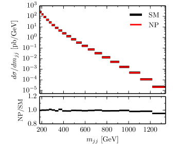
Figure 5: The dijet cross-section distribution at CDF.

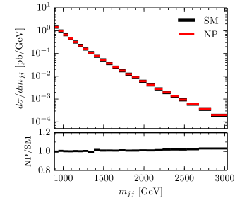
Figure 6: The dijet cross-section distribution at CMS.

In Figures 5 and 6 we compare the benchmark and SM $d\sigma_{jj}/dm_{jj}$ dijet mass spectra at the Tevatron and LHC (8 TeV). The dijet cross sections are calculated at the partonic level at LO, using ${\tt MadGraph}$ with ${\tt CTEQ6M}$ and NLO $\alpha_{s}$. Guided by the experimental analyses Aaltonen et al. (2009); Chatrchyan et al. (2013a) we impose the following cuts on the two outgoing partons (i.e. the two leading jets). For the Tevatron we impose $|y|<1$. For the 8 TeV LHC cross section calculation we require that the pseudorapidity difference between the two partons satisfies $\Delta\eta_{jj}<1.3$, and that $|\eta|<2.5$, $p_{T}>30$ GeV for each of them. The renormalization scale is set to the average $p_{T}$ of the outgoing partons in both cases. In the LHC analysis the dijet mass is above $m_{jj}>890$ GeV.

The upper two panels in Figures 5 and 6 show $d\sigma_{jj}/dm_{jj}$ in the SM (black line) and in our benchmark (red line). The lower two panels show the ratios of the two, $(d\sigma_{jj}^{NP}/dm_{jj})/(d\sigma_{jj}^{SM}/dm_{jj})$. The effect of the new resonance exchanges is small, lying below the experimental uncertainties at both the Tevatron and the LHC. In both cases the experimental analysis was aimed at bounding resonance production in the dijet channel. The CDF bump hunting analysis allows for about a $1\%$–$2\%$ spread in the ratio of data to a smooth background for $m_{jj}\in[200,700]$ GeV. This spread is larger than the deviation of $(d\sigma_{jj}^{NP}/dm_{jj})/(d\sigma_{jj}^{SM}/dm_{jj})$ from 1, as shown in the lower panel of Figure 5. Furthermore, our benchmark does not show any bumps in the spectrum at this level of precision. The CMS bump-hunting analysis allows for a NP contribution in the $m_{jj}$ spectrum at the level of a few per mill at $m_{jj}\sim 1000$ GeV, with an increase to ${\mathcal{O}}(10\%)$ at $m_{jj}\sim 3000$ GeV. Note that the benchmarks differential distribution is very smooth. Fitting $d\sigma_{jj}^{NP}/dm_{jj}$ to the same analytical function that was used to describe the smooth QCD background in Ref. Chatrchyan et al. (2013a), we find that the difference between the fit and the prediction is always well below a per mill. Thus, the bump-hunting analysis is not sensitive to our model.

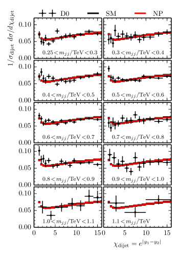
Figure 7: The dijet angular distributions at the Tevatron, in bins of $m_{jj}$. The SM predictions are denoted by black lines, the benchmark predictions in red, while measurements are denoted with crosses of the size of error bars.

CMS and DØ  have also measured the dijet angular distributions $d\sigma/d\chi$ as functions of the dijet mass (here $\chi=\exp(|y_{1}-y_{2}|)$, where $y_{1}$ and $y_{2}$ are the rapidities of the two leading jets) Abazov et al. (2009); Chatrchyan et al. (2012b). The comparison of our benchmark and SM predictions are shown in Figure 7 for the Tevatron and in Figure 8 for the LHC. The predictions are calculated at LO at the partonic level using Madgraph with CTEQ6M pdfs, setting the renormalization scale to the average $p_{T}$ of the outgoing partons. Following the DØ  analysis, we impose the Tevatron cut $y_{\rm boost}\equiv 0.5|y_{1}+y_{2}|<1$, where $y_{1,2}$ are now the rapidities of the two partons (as opposed to the rapidities of the two leading jets). The DØ  measurements begin at $m_{jj}>250$ GeV. Following the CMS angular analysis, we impose the LHC cut $y_{\rm boost}<1.11$. The CMS measurements begin at $m_{jj}>400$ GeV. The contributions from the NP resonances lead to deviations from the SM predictions that are much smaller than the experimental error bars. In the figures we show the LO predictions for the SM, however the NLO predictions are available Nagy (2002, 2003). They further improve the agreement between the data and the SM predictions. Our conclusion that the NP contributions to the angular distributions are negligible is not expected to change when going from LO to NLO predictions.

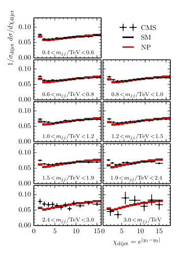
Figure 8: The angular distributions in dijet production at the LHC, measured in bins of $m_{jj}$ as indicated in the plots. The SM prediction is denoted by black lines, the prediction with our benchmark NP in red, while crosses denote the measured spectra including errors.

Another constraint arises from searches for pair production of resonances that decay to dijets, resulting in 4-jet final states. In our model this signal would be due to s-channel $\rho$ production followed by $\rho\to\pi\pi$ decays with $\pi\to jj$. The 95% CL bound on $\sigma(p\bar{p}\to X\to YY\to jj\;jj)$ from CDF for $m_{X}=175$ GeV and $m_{Y}=50(70)$ GeV is $66.8(111.5)$ pb Aaltonen et al. (2013c). In our benchmark, $X=\rho$ with a mass of $177$ GeV and $Y=\pi$ with a mass of $62$ GeV. The inclusive production cross section at LO is $\approx 79$ pb. However, after imposing partonic cuts based on the CDF hadronic jet cuts ($p_{T}^{\text{min}}>15$ GeV and $|\eta|<2.4$) we obtain $\sigma(p\bar{p}\to\rho\to\pi\pi\to jj\,jj)=37\,$ pb. The $O(\alpha_{s})$ $Z^{\prime}$ production $K$-factor, $1+8\pi\alpha_{s}(\mu)/9$, increases this cross section by $\approx 30\%$ (at $\mu=m_{\rho}=177$ GeV) to 48 pb. The analyses of pair production of dijets at CMS and ATLAS probe $m_{jj}>250$ GeV and $m_{jj}>150$ GeV Chatrchyan et al. (2013b); Aad et al. (2013b), respectively, and are thus not sensitive to the $pp\to\rho\to\pi\pi$ mode in our model. However, they could be relevant for production of higher resonances, which we cover in the next section.

III.5 Production of new states

In this section we discuss existing constraints on the production of HC resonances in our model. As already mentioned, the CDF Aaltonen et al. (2012), CMS Chatrchyan et al. (2012c) and ATLAS ATL (2012b) collaborations have searched for $t+j$ resonances, which could, in principle, constrain associated $K^{*}t$ and $K_{1}t$ production. The CDF and ATLAS analyses put bounds on $t+j$ resonance masses above $m_{tj}>200$  GeV, and are thus relevant for our model (the CMS obtains bounds for $m_{tj}>400$ GeV). The associated $K^{*}t$ and $K_{1}t$ cross sections are listed in Table 9. Here we sum over the CP conjugate final states $K^{*}t$ and $\bar{K}^{*}\bar{t}$ as well as over the light flavors, $K_{13}^{*}\sim[Q_{1}\bar{Q}_{3}]$ and $K_{23}^{*}\sim[Q_{2}\bar{Q}_{3}]$, and similarly for the $K_{1}$. At the 7 TeV LHC one has $\sigma_{K^{*}t}\,Br_{K^{*}\to\bar{t}j}=4.4$ pb, which is roughly a factor of 5 below the ATLAS bound for $m_{K^{*}}=211$ GeV ATL (2012b). At the Tevatron $\sigma_{K^{*}t}Br_{K^{*}\to\bar{t}j}=0.07$ pb, which is roughly an order of magnitude smaller than the CDF bound Aaltonen et al. (2012). In the case of associated $K_{1}$ production the products $\sigma_{K_{1}t}\,Br_{K_{1}\to\bar{t}j}$ lie even further below the corresponding bounds at the Tevatron and the LHC.

Associated $Kt$ production leads to a $\bar{t}^{*}tj$ final state, with one of the top quarks off-shell. This feeds into the experimental measurements of the (inclusive) $t\bar{t}$ cross sections Chatrchyan et al. (2014b); ATL (2013b); CMS (2012) and the $Wt$ production cross section Chatrchyan et al. (2013c); ATL (2013c). The $Kt$ cross section is comparable to the theory error on the SM prediction for $t\bar{t}$ production. Furthermore, since the $t^{*}$ is off-shell, only a fraction of the $Kt$ signal spills over into the $t\bar{t}$ production cross-section measurements. For instance, using a LO Madgraph analysis and imposing the experimental cuts for the $t\bar{t}$ signal region employed in the recent CMS dileptonic analysis Chatrchyan et al. (2014b), we estimate the $Kt$ contribution to the $8$ TeV $t\bar{t}$ cross section to be below $11$ pb. It is thus smaller than the error on the measurement $\sigma(pp\to t\bar{t})=239\pm 13$ pb Chatrchyan et al. (2014b). The softer $Kt$ lepton $p_{T}$ significantly reduces the leakage into the signal region. Similarly, the $Kt$ contribution to the $Wt$ production signal region in the recent CMS dilepton analysis at 7 TeV is below $1.7$ pb, to be compared with the CMS measurement of $\sigma(pp\to Wt)=16^{+5}_{-4}$ pb Chatrchyan et al. (2013c).

Final state	$\sigma_{\rm TEV}$	$\sigma_{\rm LHC7}$	$\sigma_{\rm LHC8}$	$\sigma_{\rm LHC13}$
$Kt$	0.38	18.0	24.2	64.5
$K^{*}t$	0.22	13.6	18.5	50.6
$K_{1}t$	0.11	11.1	15.4	45.1

Table 9: Inclusive cross sections for $pp\to K_{\text{HC}}^{(*)}t$ and $pp\to K_{1}^{(*)}t$ associated production at the Tevatron, LHC 7TeV, 8TeV and 13TeV (in pb). Summation over the first two generations ${\cal Q}_{1,2}$ and the CP-conjugate modes is assumed.

	[7 TeV]	[8 TeV]	[13 TeV]
$\sigma$ (pb)	0.54	0.92	4.39

Table 10: Cross sections for LHC pair production of the HC scalars ${\cal S}$ ${\cal S}^{*}$, at various center-of-mass energies.

Next we move to pair production of the colored scalars, ${\cal S}{\cal S}^{*}$. As discussed in Section II.3 the decay width of the ${\cal S}$ is almost an order of magnitude greater than the HC hadronization scale $\Lambda_{\rm HC}\sim{\mathcal{O}}({\rm few})f_{\pi}$. Therefore the ${\cal S}$ scalars decay before they can hadronize. This is reminiscent of the top quark in QCD. The ${\cal S}$ decays to quark–HC-quark pairs, ${\cal S}\to u_{i}\bar{\cal Q}_{i}$, where $i=1,2,3$. The ${\bar{\cal Q}}_{i}$ from ${\cal S}\to u_{i}\bar{\cal Q}_{i}$ and the ${\cal Q}_{j}$ from ${\cal S}^{*}\to u_{j}\bar{\cal Q}_{j}$ hadronize via HC strong interactions and result in final states containing many $\pi_{\rm HC}$, $K_{\rm HC}$. In general we expect $pp\to{\cal S}{\cal S}^{*}\to u_{i}\bar{u}_{j}X_{\bar{\cal Q}_{i}{\cal Q}_{j}}$, where $X_{\bar{\cal Q}_{i}{\cal Q}_{j}}$ is the multi-$\pi$, $K$ state. The light $\pi$ will receive sizable boosts. Thus, a $\pi\to jj$ decay will on average appear as a single “fat jet” in the detector. However, “fat jets” from the heavier $K\to t^{*}+j$ decays should be easier to resolve.

The ${\cal S}{\cal S}^{*}$ production cross section is $2.7$ pb in the narrow-width approximation. Taking into account the large ${\cal S}$ decay width ($\Gamma_{\cal S}\approx 0.44M_{\cal S}$), we find that the $pp\to{\cal S}{\cal S}^{*}\to u_{i}\bar{u}_{j}X_{\bar{\cal Q}_{i}{\cal Q}_{j}}$ cross section is reduced to $1.4$ pb in ${\tt MadGraph}$. The dominant contributions are $pp\to{\cal S}{\cal S}^{*}\to q_{1,2}\bar{t}\,X_{\bar{\cal Q}_{1,2}\,{\cal Q}_{3}}$ and the CP conjugate modes, with a total cross section of $0.66$ pb, and $pp\to{\cal S}{\cal S}^{*}\to t\bar{t}X_{\bar{\cal Q}_{3}{\cal Q}_{3}}$ with a cross section of $0.57$ pb. In Figure 9 we show the mass distributions for $pp\to{\cal S}{\cal S}^{*}\to q_{1,2}\,\bar{t}\,X_{\bar{\cal Q}_{1,2}{\cal Q}_{3}}$; the distributions for the other decay modes of the ${\cal S}$ are very similar. One can see that the bulk of the $X_{\bar{\cal Q}_{1,2}{\cal Q}_{3}}$ system has invariant masses that lie above $\Lambda_{\chi}\sim{\mathcal{O}}(250)$ GeV, and also well above the threshold for multi-pion production. There is enough energy available to produce $tjK$, $tjK+\pi$, $tjK+2\pi$, etc, multi-pion final states. The cross section for producing one, two, three, or more HC pions depends on the details of the HC dynamics, and thus on the hadronization model. One could contemplate rescaling the hadronization models used for QCD to the HC scale to obtain a more quantitative description. However, for our purposes a qualitative picture suffices.

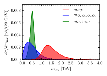
Figure 9: The invariant mass distributions for $pp\to{\cal S}{\cal S}^{*}\to q_{1,2}\bar{t}X_{\bar{\cal Q}_{1,2}{\cal Q}_{3}}$. The ${\cal S}{\cal S}^{*}$ pair invariant masses are in red, the $X_{\bar{\cal Q}_{1,2}{\cal Q}_{3}}$ HC multipion invariant masses are in blue, and the individual invariant mass distributions of the ${\cal S}$ and ${\cal S}^{*}$ are similar and shown in green.

If we were to model the hadronization of the $\bar{\cal Q}_{1,2}{\cal Q}_{3}$ pair with a string model, the extra pions would be created from string breaking. Since there is sufficient energy, the penalty for creating an extra pion is small. As we saw, pair production of ${\cal S}{\cal S}^{*}$ would result in $tj+n$ fat jets (the HC pions and kaons) or $t\bar{t}+n$ fat jets final states. Here $n$ can lie anywhere from 1 to ${\mathcal{O}}(10)$. The ${\cal S}{\cal S}^{*}$ pair can thus be searched for in multijet final states. Both the CMS and ATLAS collaborations have recently made significant progress in multijet searches Aad et al. (2012); Chatrchyan et al. (2014c); ATL (2013d). Particularly relevant in this respect is the ATLAS search ATL (2013d), which was interpreted in terms of gluino production with R-parity violating decays that result in either 6-jet or 10-jet final states (in the 6-jet search an extra initial-state radiation jet was required in order to optimize the sensitivity). Most importantly, the search strategy did not require the jets to form resonances of a particular mass, and can thus be used to place bounds on the production of wide resonances, such as ${\cal S}{\cal S}^{*}$. For a $520$ GeV gluino that decays to $tjj$ the ATLAS bound is $\sigma(pp\to\tilde{g}\tilde{g}\to\bar{t}t+4j)<0.9$ pb. This bound lies above the cross section for $\sigma(pp\to{\cal S}{\cal S}^{*}\to t\bar{t}+n\pi)$ in our model.

The ATLAS collaboration has also performed a search in which the final state contains $t\bar{t}+2b$ jets and a number of light jets. This final state arises in our model from $pp\to{\cal S}{\cal S}^{*}\to t\bar{t}\,K\bar{K}$ plus any number of other pNGBs (a much smaller contribution could come from the $\phi$ resonance in place of $K\bar{K}$). Here, the hadronization of HC quarks results in a $K\bar{K}$ pair. The kaons then decay to off-shell $t^{*}$, so that $K\to t^{*}j\to b\,3j$. We thus have $pp\to{\cal S}{\cal S}^{*}\to t\bar{t}\,2b\,6j$. The ATLAS search ATL (2013d), with a gluino decaying to five quarks through an intermediate neutralino, gives an upper bound of about $1.5$ pb, well above our production cross section of $0.6$ pb.

IV Electroweak precision tests, Higgs couplings

In this section we discuss the implications of electroweak-precision measurements for our model. For the contributions to the electroweak oblique parameters $S$ and $T$ due to new HC states we rely on the operator product expansion (OPE) and quark hadron duality in order to estimate these contributions. Thus, the electroweak corrections are given by the diagrams in Figure 10 to good approximation. The corrections are suppressed by powers of $\Lambda_{\rm HC}/m_{\cal S}$. The scalar $\mathcal{S}$ is an ${\rm SU}(2)$ singlet and thus does not contribute to the $S$ parameter. The contribution to the $T$ parameter, on the other hand, vanishes due to a cancellation between the two diagrams shown in Figure 10 (see also the discussion of models with Higgs singlets in Ref. Grimus et al. (2008)). The HC quarks are hypercharge singlets and thus do not contribute at this order.

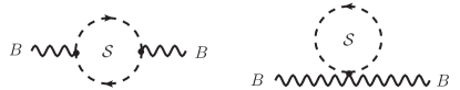
Figure 10: The two contributions of the scalar $\mathcal{S}$ to the $T$ parameter cancel.

In Ref. Gresham et al. (2012b) atomic-parity violation was advocated as a strong constraint on t-channel explanations of the forward-backward asymmetry. Below the electroweak scale atomic-parity violation can be described by an effective electron-quark interaction of the form

$${\mathcal{L}}=\frac{G_{F}}{\sqrt{2}}\sum_{q=u,d}\big{(}C_{1q}\bar{e}\gamma^{\mu}\gamma_{5}e\bar{q}\gamma_{\mu}q+C_{2q}\bar{e}\gamma^{\mu}e\bar{q}\gamma_{\mu}\gamma_{5}q\big{)}\,,$$ (56)

where the second term is suppressed by the small electron weak charge and neglected in the following. We define the $Z$–light-quark couplings as in Ref. Gresham et al. (2012b) by

$${\mathcal{L}}=-\frac{e}{s_{w}c_{w}}Z^{\mu}\big{(}a_{R}^{\text{NP}}(q)\bar{q}_{R}\gamma_{\mu}q_{R}+a_{L}^{\text{NP}}(q)\bar{q}_{L}\gamma_{\mu}q_{L}\big{)}\,.$$ (57)

In terms of the effective electron-quark Wilson coefficients we have $C_{1q}^{\text{NP}}=a_{L}^{\text{NP}}(q)+a_{R}^{\text{NP}}(q)$.

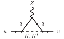
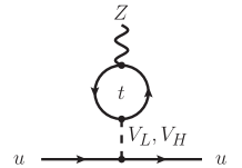
Figure 11: Vector and pseudoscalar meson contribution to atomic-parity violation.

To estimate the effect of the $K^{*}$ resonances on atomic-parity violation, we compute the matching corrections to $a_{R}^{K^{*}}(u)$. To this end we evaluate the diagrams with the exchange of a massive vector and a top quark (cf. Figure 11). The finite part of the contribution of the $K^{*}$–top-quark loops, including field renormalization, is

$$\begin{split}a_{R}^{K^{*}}(u)&=\frac{g_{\rho}^{2}\sin^{2}\theta_{R,1}\sin^{2}\theta_{R,3}}{32\pi^{2}}\\ &\quad\times\Big{[}\frac{x^{2}-7x}{8(x-1)}+\frac{3x\log x}{4(x-1)^{2}}-\frac{x}{4}\log\frac{\mu^{2}}{m_{t}^{2}}\Big{]}\,,\end{split}$$ (58)

where $x\equiv m_{t}^{2}/m_{K^{*}}^{2}$. Note that the $K^{*}$ contribution is divergent because of our use of a non-gauge vector propagator. The divergent contribution vanishes in the limit $x\to 0$. We estimate the size of the effect by varying the renormalization scale, $\mu$, in the range $[M_{K^{*}}/2,2M_{K^{*}}]$. The same expression also applies for $K_{1}$ exchange with $x\to m_{t}^{2}/m_{K_{1}}^{2}$ and $g_{\rho}\to g_{a_{1}}$.

The effect of HC $K$ exchange is similarly estimated by evaluating the diagram in Figure 11 with $K$ in the loop. The finite part of the contribution of the $K$–top-quark loops, including field renormalization, is given by

$$\begin{split}a_{R}^{K}(u)&=\Big{(}\frac{g_{A}^{\text{HC}}}{f_{\pi}^{\text{HC}}}\Big{)}^{2}\frac{\sin^{2}\theta_{R,1}\sin^{2}\theta_{R,3}}{32\pi^{2}}M_{K}^{2}\\ &\quad\times\Big{[}\frac{x+x^{2}}{8(1-x)}+\frac{x\log x}{4(x-1)^{2}}+\frac{x}{4}\log\frac{\mu^{2}}{m_{t}^{2}}\Big{]}\,,\end{split}$$ (59)

where $x\equiv m_{t}^{2}/M_{K}^{2}$. Note that this contribution is divergent because of the dimension-five couplings in Eq. (36). As in the case of the $K^{*}$ above, the divergent contribution vanishes in the limit $x\to 0$, and the size of the effect is estimated by varying the renormalization scale in the range $[M_{K}/2,2M_{K}]$. All contributions of the $K^{*}$ and $K$ loops proportional to the weak mixing angle vanish after renormalizing the external fermion fields.

The contribution of the top-quark loop diagram in Figure 11 (right) is given by

$$\begin{split}a_{R}^{V_{H,L}}(u)&=\mp\frac{g_{\rho}^{2}\sin^{2}\theta_{R,1}\sin^{2}\theta_{R,3}}{32\sqrt{2}\pi^{2}}\sin\theta_{V_{H,L}}^{\text{id}}\cos\theta_{V_{H,L}}^{\text{id}}\\ &\quad\times N_{c}\Big{[}\frac{m_{t}^{2}}{m_{V_{H,L}}^{2}}\log\frac{\mu^{2}}{m_{t}^{2}}\Big{]}\,.\end{split}$$ (60)

This is substantially suppressed by the small deviation from the ideal $\omega-\phi$ mixing, $\sin\theta_{V}^{\rm id}=0.028$ defined in Eq. (15) (see also Appendix A). The analogous contribution from axial $A_{L}-A_{H}$ exchange is obtained by replacing $\theta_{V_{H,L}}^{\text{id}}\to\theta_{V,A}^{\text{id}}$, $g_{\rho}\to g_{a_{1}}$, $m_{V_{H,L}}\to m_{V,A}$. As above, the scale $\mu$ in Eq. (60) and the axial-vector analog is varied in the range of half to twice the resonance mass.

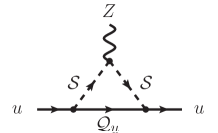
Figure 12: Contribution of the heavy scalar ${\cal S}$ to atomic-parity violation.

Finally, we estimate the effect of the would-be composite quarks on atomic-parity violation. As discussed in Section II.3, they are closely analogous to a heavy-light meson. In our case the role of the heavy quark is played by the heavy scalar. We thus evaluate the corresponding loops in the UV theory, as shown in Figure 12. The $Z$ coupling to the scalar is given in terms of the covariant derivative

$$D_{\mu}=\partial_{\mu}+\frac{2}{3}\frac{ies_{w}}{c_{w}}Z_{\mu},$$ (61)

in the kinetic term

$${\cal L}_{\text{kin}}=\big{(}D_{\mu}{\cal S}\big{)}^{\dagger}D^{\mu}{\cal S}\,.$$ (62)

We find that the contribution of the renormalized diagram vanishes.

We can obtain a bound on the size of $a_{R}^{\text{NP}}(u)$ from the measurement of the nuclear weak charge of cesium (${}^{133}\text{Cs}$). The contribution of $a_{R}^{\text{NP}}(u)$ to the nuclear weak charge is given by

$$\Delta Q_{W}=-2(2Z+N)a_{R}^{\text{NP}}(u)\,,$$ (63)

where $Z$ and $N$ are the number of protons and neutrons in the nucleus. From the difference of the experimental value, $Q_{W}^{\text{exp}}=-72.58(43)$ Dzuba et al. (2012), and the central value of the SM prediction $Q_{W}^{\text{SM}}=-73.23$ (calculated with input from Ref. Beringer et al. (2012)),

$$\Delta Q_{W}(\text{Cs})\equiv Q_{W}^{\text{exp}}(\text{Cs})-Q_{W}^{\text{SM}}(\text{Cs})\subset[0.22,1.08],$$ (64)

we obtain the allowed 1-sigma region $a_{R}^{\text{NP}}(u)\subset[-0.28,-0.06]\%$. This should be compared with the HC resonance contributions listed in Table 11. One sees that the HC effects are well within the errors on $a_{R}^{\rm NP}$.

The HC interactions modify the Higgs production cross sections and decays branching ratios. However, we find these modifications to be small in size. The effects of the quartic Higgs coupling to scalar ${\cal S}$ are suppressed by its large mass, $m_{\cal S}$, and are negligible. Modifications of the Higgs couplings to the $W$ and $Z$ arise at loop level and are irrelevant. In principle the partial compositeness of the RH top quark could lead to appreciable modifications in $\bar{t}th$ production, $gg\to h$ fusion, and the $h\to\gamma\gamma$ decay channel, via the RH and LH mixings in Eqs. (29), (30). The $\bar{t}th$ production cross section is given by

$$\frac{\sigma_{\bar{t}th}^{\rm NP}}{\sigma_{\bar{t}th}^{\rm SM}}=\Big{(}\frac{y_{t}^{\rm NP}}{y_{t}^{\rm SM}}\Big{)}^{2}\cos\theta_{R3}^{2}\cos\theta_{L3}^{2}=1+{\mathcal{O}}(1/M^{4})\,,$$ (65)

where $y_{t}^{\rm NP}\equiv m_{u_{3}}/v$ is the top-quark Yukawa coupling in the interaction basis, which differs from the SM relation $y_{t}^{\rm SM}=m_{t}^{\rm phys}/v$. Since the physical top-quark mass is given by $m_{t}^{\rm phys}\simeq m_{u_{3}}\cos\theta_{R3}\cos\theta_{L3}$ the net change in the $t\bar{t}h$ production cross section is small. Numerically, it is an ${\mathcal{O}}(1\%)$ effect.

In the limit of a heavy top, where the Higgs low-energy theorem applies, the contributions of the top and the would-be composite top quark $u^{\prime}_{3}$ running in the loop completely cancel in the $gg\to h$ and $h\to\gamma\gamma$ amplitudes. The net modifications of the gluon-fusion cross section and the $h\to\gamma\gamma$ branching ratio therefore lie well below a percent.

	1-$\sigma$ range [%]
$a_{R}^{K}(u)$	$[-0.215,0.010]$
$a_{R}^{K^{*}}(u)$	$[-0.037,-0.005]$
$a_{R}^{K_{1}}(u)$	$[-0.054,-0.023]$
$a_{R}^{V_{L}}(u)$	$[-0.0008,0.0009]$
$a_{R}^{V_{H}}(u)$	$[-0.0002,0.0007]$

Table 11: Range of the effective $a_{R}$ coupling to $Z$ in %, induced by the HC resonance contributions discussed in the main text.

V The signals of stealth strong dynamics

Our strong interaction model for enhanced $t\bar{t}$ asymmetries makes several predictions that are not tied to the exact numerical values of the UV parameters and are thus quite robust. It predicts the existence of a tower of resonances that couples strongly to the right-handed top $t_{R}$: $K,K^{*},K_{1},...$ There is a flavor octet of pNGBs: $\pi,K,\eta$ (plus the $\eta^{\prime}$), with the lightest state decaying to two jets. The latter is most likely a triplet of pions, with a mass of $\sim 50$ GeV. Finally, the minimal form of the model also predicts the existence of a stable, electrically neutral “HC baryon” with a mass of $\sim 250$ GeV, which may be searched for in direct dark matter (DM) detection experiments.

The HC resonances $K^{*},K_{1},...$ decay to $t+j$ final states and are already being searched for, as discussed in Section III.5. Their production cross section will increase roughly $4$-fold in going from the 8-TeV LHC to the 13-TeV LHC, see Table 9. This should be compared with the corresponding $\sim 5$-fold increase in the $t\bar{t}$ cross section. The challenge will be to search for $t+j$ resonances given the larger hadronic activity in 13-TeV events. One could explore the fact that, at 13 TeV, the anti-top quarks in $pp\to t+K^{*}\to t\bar{t}j$ will in general be produced at larger rapidities than the anti-top quarks in $t\bar{t}$ events (see Figure 13). The usefulness of this charge asymmetry at the LHC has been discussed in Ref. Knapen et al. (2012) for the case of associated $W^{\prime}t$ production.

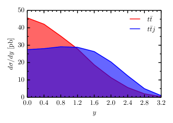
Figure 13: The rapidity distribution of the anti-top quark from $pp\to t\bar{t}$ (red) and $pp\to tK^{*}\to t\bar{t}j$ (blue), for LHC at 13 TeV. The $pp\to t\bar{t}j$ differential cross section has been rescaled by a factor $20$.

Next, we discuss searches for HC $K$ mesons. A challenge here is that the $K$ decays to an off-shell top, $K\to t^{*}j$. Ideally, the present experimental searches would be optimized to search not just for $t+j$ resonances but also for $t^{*}+j$ resonances. Gains are potentially possible, if one allows for softer leptons from the semileptonic decays of the $t^{*}$.

The discovery of a light pion decaying to two jets would be a particularly striking signal of stealth strong dynamics. The challenge in searching for HC pions is that they are most copiously produced in decays of higher resonances, which typically results in high multiplicity final states. An exception is the HC $\rho$ resonance, which almost exclusively decays through $\rho\to\pi\pi$. The s-channel production $pp\to\rho\to\pi\pi$, with $\pi\to 2j$ is effectively already searched for in paired dijet events, as discussed in Section III.4. However, in our model both $\rho$ and $\pi$ are very light, thus present searches are not sensitive to them. It is unlikely that the sensitivity to the low-mass region can be improved in this type of search at the LHC with increased collision energies. Potentially more promising may be the pair production of $\rho$ resonances, $pp\to\rho\rho\to 4\pi$, in which each pion decays to two jets. Since the $\rho$’s would come primarily from the partonic $u\bar{u}\to\rho\rho$ process, with the $u$ quark in the t-channel, they would have large rapidities.

The cross sections for the process $pp\to\rho\rho$ are $0.38$ pb at LHC8 and $1.38$ pb at LHC13, respectively. A promising search strategy would thus be to optimize a search for forward pair production of resonances, resulting in two fat jets (potentially further resolved into two jets each using jet substructure techniques).

Finally, our model in its minimal form of Eq. (2) contains a stable neutral HC baryon $B_{\chi}$ formed from three of the light HC quarks. The Lagrangian is invariant under a global ${\rm U}(1)_{{\rm\cal B}_{\rm HC}}$ HC baryon-number symmetry, under which the HC quarks ${\cal Q}_{i}$ have charge ${\rm\cal B}_{\rm HC}=1/3$, ${\cal S}$ has charge ${\rm\cal B}_{\rm HC}=-1/3$, while all gauge and SM-matter fields are neutral. Alternatively, one can consider the $Z_{2}^{\rm HC}$ subgroup, under which the HC quarks and ${\cal S}$ are odd, and the SM matter is even. The lightest HC baryon state $B_{\chi}$ (${\rm\cal B}_{\rm HC}=1$, or $Z_{2}^{\rm HC}$ odd) is therefore stable. We estimate its mass by rescaling from QCD, yielding $m_{B_{\chi}}\sim m_{p}\,f_{\pi}^{\rm HC}/f_{\pi}^{\rm HC}\sim 220$ GeV, not including the HC quark-mass contributions.

Small breaking of the flavor ${\rm U}(2)_{U_{R}}$ symmetry should be accompanied by small mass splittings between the light HC quarks, with $m_{{\cal Q}_{2}}>m_{{\cal Q}_{1}}$ or $m_{{\cal Q}_{2}}<m_{{\cal Q}_{1}}$. We therefore consider two possible flavor structures for the lightest HC baryon, $B_{\chi}[{\cal Q}_{1}{\cal Q}_{1}{\cal Q}_{2}]$ or $B_{\chi}[{\cal Q}_{2}{\cal Q}_{2}{\cal Q}_{1}]$, respectively. In general, we expect the two baryons in this “isospin doublet” to be nearly degenerate in mass, since the ${\rm U}(2)_{U_{R}}$ symmetry must remain approximately intact due to FCNC constraints.

If $B_{\chi}$ is a thermal relic, its relic abundance is set by its annihilation cross section in the early universe. This is dominated by $B_{\chi}\overline{B}_{\chi}\to$ multi-$\pi_{\rm HC}$ final states. We estimate this by scaling the QCD $p\bar{p}$ annihilation cross section to the HC scale,

$$\sigma_{B_{\chi}\overline{B}_{\chi}}\approx\sigma_{p\bar{p}}\,(f_{\pi}^{\rm HC}/f_{\pi})^{2}\,.$$ (66)

The $p\bar{p}$ annihilation cross sections measured by the LEAR collaboration Bruckner et al. (1990) vary from $\approx 200$ mb to $\approx 80$ mb, for $\bar{p}$ beam momenta varying from $200$ MeV to $\approx 600$ MeV, respectively. Using Eq. (66) and converting the LEAR $\bar{p}$ beam momenta to center of mass values of $v/c$, we obtain the range of $B_{\chi}$ annihilation cross sections $\sigma_{B_{\chi}\overline{B}_{\chi}}\approx 0.01$ mb ($v/c\approx 0.1$) to $\sigma_{B_{\chi}\overline{B}_{\chi}}\approx 0.004$ mb ($v/c\approx 0.3$). Note that the non-relativistic values of $v/c$ are in the range relevant for estimating thermal relic DM abundances. In particular, we find $\langle\sigma_{B_{\chi}\overline{B}_{\chi}}\,v\rangle\sim 3\cdot 10^{-20}~{}{\rm cm^{3}/s}$. This is $10^{6}\times\langle\sigma v\rangle_{\rm th.rel.}$, where $\langle\sigma v\rangle_{\rm th.rel.}=3\cdot 10^{-26}\text{cm}^{3}/s$ would be the annihilation cross section required for $B_{\chi}$ to explain the observed DM abundance.

Our estimate for $\langle\sigma_{B_{\chi}\overline{B}_{\chi}}\,v\rangle$ implies that the $B_{\chi}$ would be a very subleading DM component, with $\Omega_{B_{\chi}}\sim{\mathcal{O}}(10^{-6})\times\Omega_{\rm DM}$. Nevertheless, DM direct detection searches could be sensitive to it, because the $B_{\chi}$-nucleon scattering cross section is large. The latter is dominated by exchange of the vector mesons $\rho_{HC},V_{L}(\omega_{\rm HC})$. For simplicity, we only consider the vector couplings $g_{V}\overline{B}_{\chi}\gamma_{\mu}B_{\chi}V^{\mu}$, and ignore the higher-dimension tensor couplings. For the coupling strengths, we use the corresponding QCD sum-rule values Erkol et al. (2006): $g_{\rho}=2.3$ and $g_{\omega}=6.9$.

For $B_{\chi}[{\cal Q}_{1}{\cal Q}_{1}{\cal Q}_{2}]$, its cross section with protons is given by

$$\sigma(B_{\chi}\,p\to B_{\chi}\,p)=(\kappa_{R}^{\rho})^{2}{(g_{\rho}+g_{\omega})^{2}\over m_{\rho_{\rm HC}}^{4}}{m_{p}^{2}\over 16\pi}\,,$$ (67)

where we have ignored the small splitting between the $\rho_{\rm HC}$ and $V_{L}$ masses, and the couplings of the $\rho_{\rm HC}$ and $V_{L}$ to the RH up quark are equal and given by $\kappa^{\rho}_{R}=0.117$, see Table 8. For $B_{\chi}[{\cal Q}_{2}{\cal Q}_{2}{\cal Q}_{1}]$, its cross section with protons is obtained by substituting $g_{\rho}\to-g_{\rho}$ in Eq. (67). In both cases the cross sections with neutrons are a factor of four smaller. Thus, for our benchmark we estimate that the $B_{\chi}$–nucleon cross section would be $\sigma_{\rm scatt}\sim 10^{-38}~{}{\rm cm}^{2}$ for $B_{\chi}[{\cal Q}_{2}{\cal Q}_{2}{\cal Q}_{1}]$, and $\sigma_{\rm scatt}\sim 5\cdot 10^{-38}~{}{\rm cm}^{2}$ for $B_{\chi}[{\cal Q}_{1}{\cal Q}_{1}{\cal Q}_{2}]$. The LUX bound on the DM-nucleon scattering cross section excludes $(\Omega_{B_{\chi}}/\Omega_{\rm DM})\times\sigma_{\rm scatt}\lesssim 2.5\cdot 10^{-45}\,\text{cm}^{2}$ Akerib et al. (2013) for $m_{B_{\chi}}\sim 220$ GeV. With our estimate for $\Omega_{B_{\chi}}/\Omega_{\rm DM}$, the scattering of relic $B_{\chi}[{\cal Q}_{2}{\cal Q}_{2}{\cal Q}_{1}]$ on nuclei would seem to be at the very limit of the allowed range, whereas for $B_{\chi}[{\cal Q}_{1}{\cal Q}_{1}{\cal Q}_{2}]$ it is an order of magnitude too large. The uncertainties in our estimates of the $B_{\chi}$ relic density and cross sections with nucleons are large and warrant a more detailed analysis to see whether or not stealth strong dynamics could be discovered in direct DM searches.

Finally, we point out that the HC baryon number (or discrete $Z_{2}^{\rm HC}$) symmetry is accidental and therefore may only be approximate. For instance, it could be broken at some higher scale in extensions of our model with a larger field content. In that case all of the HC baryons could be unstable and decay in the early universe. For example, if the SM is extended by a light right-handed neutrino, $\nu_{R}$, the breaking can exhibit itself through a dimension-seven operator $({\cal S}^{\dagger}{\cal Q}_{1}{\cal Q}_{2})u_{R}\nu_{R}$ which also breaks the ${\rm U}(2)_{U_{R}}$ symmetry, where the ${\rm SU}(N)_{\rm HC}$ indices in the bracket are contracted with the antisymmetric Levi-Civita tensor.

VI Conclusions

We have provided an explicit strong interaction model that can produce large enhancements of the $t\bar{t}$ asymmetries at the Tevatron, while not being excluded by other direct or indirect searches for new physics. The model minimally extends the SM field content by a (SM gauge singlet) flavor triplet of vectorlike fermions ${\cal Q}_{i}$ charged under a new strong gauge group, and by a scalar ${\cal S}$ charged under QCD, hypercharge and the new strong gauge group. We choose ${\rm SU}(3)_{\rm HC}$ “hypercolor” for the strong gauge group in order to directly translate the results of QCD strong dynamics, thus reducing the uncertainties in our predictions. An approximate ${\rm U}(2)$ flavor symmetry is imposed on the fundamental interactions between the hypercolor and SM sectors – the Yukawa-type couplings of the ${\cal S}$ to the RH up quarks and ${\cal Q}_{i}$. The ${\cal Q}_{i}$ masses are also ${\rm U}(2)$ invariant, and satisfy a hierarchy analogous to $m_{u,d}\ll m_{s}\sim f_{\pi}$ in QCD. The ${\cal S}$ is heavier, and is thus analogous to a heavy flavor quark in QCD with mass $m\gg 4\pi f_{\pi}$. The flavor symmetry insures that new physics contributions to flavor-changing neutral currents, e.g., $D^{0}$–$\overline{D^{0}}$ mixing or same-sign top pair production, are negligible or absent. The fact that the HC sector is neutral with respect to the ${\rm SU}(2)_{L}$ weak interaction allows the model to easily evade precision electroweak tests, and also ensures that any modifications of the Higgs couplings are very small.

The scale of the new strong dynamics is quite low. The mass of the lightest pseudo Nambu-Goldstone boson, $\pi_{\rm HC},$ is merely $60$ GeV, while most of the remaining resonances are in the range of $\approx 150$ GeV to $\approx 300$ GeV. Despite a plethora of new resonances, the model is, surprisingly, not yet excluded by new physics searches. The reason is two-fold: (i) these resonances are bound states of the ${\cal Q}_{i}$ and are thus QCD color neutral, (ii) the heavier hypercolor scalar ${\cal S}$ rapidly decays into high-multiplicity final states, before it can form QCD colored bound states. In particular, pair production of ${\cal S}{\cal S}^{*}$ would result in $tj+n$ fat jets or $t\bar{t}+n$ fat jets final states, where a “fat jet” is associated with a $\pi_{\rm HC}\to jj$ or $K_{\rm HC}\to t^{*}j$ decay.

There already has been considerable progress at the LHC in searches for new physics involving final states with large jet multiplicities. However, searches in relatively low-multiplicity final states, including fat jets, are probably the most promising for discovery of hypercolor resonances. An example is pair production of $\rho_{\rm HC}$ resonances, with each $\rho_{\rm HC}$ decaying to a pair of HC pions, resulting in the chain $pp\to\rho_{\rm HC}\,\rho_{\rm HC}\to 4\,\pi_{\rm HC}\to 4$ fat jets. The rather strong coupling of the hypercolor sector to the top quarks leads to observable $t\bar{t}$ charge asymmetries in associated hypercolor resonance production at the LHC. This feature could be useful in discriminating signal from background in $t$+ jet resonance searches. For example, the $\bar{t}$ in the process $pp\to tK_{\rm HC}^{*}\to t\bar{t}j$ is produced with relatively large rapidities compared to the top, and compared to the anti-top in $pp\to t\bar{t}$. This feature could also be useful in virtual $t^{*}+j$ resonance searches associated with the process $pp\to tK_{\rm HC}\to t\bar{t}^{*}j$.

We have used known non-perturbative aspects of QCD, as well as familiar approximations like QCD sum rules, vector-meson dominance, and a naive quark model, combined with simple scaling arguments to obtain reasonable estimates of the resonance masses and interaction strengths in our QCD-like hypercolor model. An interesting application concerns the relic abundance of the lightest HC baryon, $B_{\chi}$. If the accidental HC baryon number symmetry of our Lagrangian is left unbroken by higher-dimensional operators involving additional light non-SM fields, then the $B_{\chi}$ is stable. Scaling the measured low-energy QCD $p\bar{p}$ annihilation cross sections will imply a $B_{\chi}$ relic abundance that is only ${\mathcal{O}}(10^{-6})$ as large as the observed dark matter abundance. Nevertheless, the $B_{\chi}$–nucleon cross section is large enough to be close to saturating the present direct dark matter detection bounds, and may yield an observable signal in the next generation of the dark matter direct detection experiments or rule out a stable $B_{\chi}$.

An interesting open question is also the UV structure of our model. The one-loop running of the Yukawa couplings $h_{1},h_{3}$ and the HC gauge coupling $g_{\rm HC}$ gives a Landau pole at $\mu=O({\rm few~{}TeV})$, whereas two-loop RGEs give an approximate UV fixed point for $h_{3}$ of non-perturbative strength, $h_{3}^{*}\approx 8$, that is realized at $\mu=O(10$ TeV), with $h_{1}$ and $g_{\rm HC}$ asymptotically free. To settle the question which of the two possibilities is realized would require nonperturbative methods, and is beyond the scope of the current work, but could be an interesting future research direction.

In summary, the presented model can lead to large $t\bar{t}$ asymmetry at the Tevatron, evades present experimental bounds, but can be searched for with improved strategies at the LHC and in direct dark matter detection experiments.

Acknowledgements: J.B. and E.S. would like thank Antonio Pich for useful discussions. We would like to thank the Weizmann Institute Phenomenology group, and the CERN theory group for their warm hospitality during various stages of this work. A. K. and J.B. are supported by DOE grant FG02-84-ER40153. J. Z. and J.B. are supported by the U.S. National Science Foundation under CAREER Grant PHY-1151392. We also thank the Aspen Center for Physics, supported by the NSF Grant #1066293, and the KITP, supported in part by the National Science Foundation under Grant No. NSF PHY11-25915, for their warm hospitality. A.K. and J.Z. are grateful to the Mainz Institute for Theoretical Physics (MITP) for its hospitality and its partial support during the completion of this work. E.S. would like to thank the Department of Physics at University of Cincinnati for its warm hospitality during the initial stages of this work.

Appendix A Resonance mass spectra

The masses of the HC mesons are obtained from the measured spectrum of QCD mesons by appropriate rescalings. To good approximation, the QCD $\rho$ mass, $m_{\rho}^{\rm QCD}$, corresponds to the massless limit of the HC $\rho$ meson, $M_{\chi}=\lim_{m_{{\cal Q}_{i}}\to 0}\,m_{\rho}^{\rm HC}$. In obtaining the spectra we also need to allow for variatons of the HC quark masses. We do this by employing ChPT for the pseudoscalar mesons and a naive quark model for the vector and axial-vector resonances.

A.1 Pseudoscalar mesons

The compositions of the HC pion and kaon in terms of the HC quarks are

$$\begin{split}|\pi^{1(2)}\rangle&=|\bar{\cal Q}_{1(2)}{\cal Q}_{2(1)}\rangle\,,\\ |\pi^{3}\rangle&={1\over\sqrt{2}}(|\bar{\cal Q}_{1}{\cal Q}_{1}\rangle-|\bar{\cal Q}_{2}{\cal Q}_{2}\rangle)\,,\\ |K^{1(2)}\rangle&=|\bar{\cal Q}_{1(2)}{\cal Q}_{3}\rangle\,,\qquad|\bar{K}^{1(2)}\rangle=|\bar{\cal Q}_{3}{\cal Q}_{1(2)}\rangle\,,\end{split}$$ (68)

while the octet and the singlet pseudoscalars are given by

$$\begin{split}|\eta_{8}\rangle&={1\over\sqrt{6}}(|\bar{\cal Q}_{1}{\cal Q}_{1}\rangle+|\bar{\cal Q}_{2}{\cal Q}_{2}\rangle-2|\bar{\cal Q}_{3}{\cal Q}_{3}\rangle)\,,\\ |\eta_{0}\rangle&={1\over\sqrt{3}}(|\bar{\cal Q}_{1}{\cal Q}_{1}\rangle+|\bar{\cal Q}_{2}{\cal Q}_{2}\rangle+|\bar{\cal Q}_{3}{\cal Q}_{3}\rangle)\,.\end{split}$$ (69)

As explained in the main text, we neglect $\eta-\eta^{\prime}$ mixing, so that the $\eta_{8}=\eta$ and $\eta_{0}=\eta^{\prime}$.

The quadratic terms in the chiral Lagrangian yield expressions for the squared pseudoscalar masses which are linear in the quark masses

$$\begin{split}\left(m_{\pi^{1,2,3}}\right)^{2}&=k_{f}\frac{M_{\chi}}{m^{\text{QCD}}_{\rho}}~{}2m_{{\cal Q}_{1}}\,,\\ \left(m_{K^{1,2},\bar{K}^{1,2}}\right)^{2}&=k_{f}\frac{M_{\chi}}{m^{\text{QCD}}_{\rho}}~{}(m_{{\cal Q}_{1}}+m_{{\cal Q}_{3}})\,,\\ \left(m_{\eta}\right)^{2}&=k_{f}\frac{M_{\chi}}{m^{\text{QCD}}_{\rho}}~{}\frac{2}{3}(m_{{\cal Q}_{1}}+2m_{{\cal Q}_{3}})\,.\end{split}$$ (70)

We use $k_{f}=2.765$ as obtained from the lattice QCD calculation in Ref. McNeile et al. (2012). The $\eta^{\prime}$ is assumed to be much heavier than the other pseudoscalar mesons and is omitted from our analysis as explained in Section II.1.

A.2 Vector Mesons

The vector meson masses and the mixing angle between the flavor-singlet and octet states are calculated using the naive quark model approach in Ref. Cheng and Shrock (2011). The decompositions of the $\rho$ and $K^{*}$ in terms of HC quark states are

$$\begin{split}|\rho^{1(2)}\rangle&=|\bar{\cal Q}_{1(2)}{\cal Q}_{2(1)}\rangle\,,\\ ~{}|\rho^{3}\rangle&={1\over\sqrt{2}}(|\bar{\cal Q}_{1}{\cal Q}_{1}\rangle-|\bar{\cal Q}_{2}{\cal Q}_{2}\rangle)\,,\\ |K^{*1(2)}\rangle&=|\bar{\cal Q}_{1(2)}{\cal Q}_{3}\rangle\,,~{}~{}|\bar{K}^{*1(2)}\rangle=|\bar{\cal Q}_{3}{\cal Q}_{1(2)}\rangle\,.\end{split}$$ (71)

Their masses are given by

$$\begin{split}\left(m_{\rho^{1,2,3}}\right)^{2}&=\mu_{V}^{\text{HC}}\left(E^{\text{HC}}_{0,V}+2m_{{\cal Q}_{1}}\right),\\ \left(m_{K^{*1,2},\bar{K}^{*1,2}}\right)^{2}&=\mu_{V}^{\text{HC}}\left(E^{\text{HC}}_{0,V}+m_{{\cal Q}_{3}}+m_{{\cal Q}_{1}}\right).\end{split}$$ (72)

Here $\mu_{V}^{\text{HC}}$ is an overall mass-scale parameter, $E_{0,V}$ describes the binding energy in the limit of massless HC quarks, while the $m_{{\cal Q}_{i}}$ are the HC quark masses.

The octet and singlet vector meson states are

$$\begin{split}|V_{8}\rangle&={1\over\sqrt{6}}(|\bar{\cal Q}_{1}{\cal Q}_{1}\rangle+|\bar{\cal Q}_{2}{\cal Q}_{2}\rangle-2|\bar{\cal Q}_{3}{\cal Q}_{3}\rangle)\,,\\ |V_{0}\rangle&={1\over\sqrt{3}}(|\bar{\cal Q}_{1}{\cal Q}_{1}\rangle+|\bar{\cal Q}_{2}{\cal Q}_{2}\rangle+|\bar{\cal Q}_{3}{\cal Q}_{3}\rangle)\,.\end{split}$$ (73)

The mixing angle between the flavor-singlet and octet vector mesons is obtained by diagonalising the corresponding mass matrix

$$\begin{split}\begin{pmatrix}\left(m_{V_{L}}\right)^{2}&0\\ 0&\left(m_{V_{H}}\right)^{2}\\ \end{pmatrix}=R_{V}\begin{pmatrix}\mu_{V}^{\text{HC}}\left(E_{0V}^{\text{HC}}+\tfrac{2}{3}(2m_{{\cal Q}_{1}}+m_{{\cal Q}_{3}})+x_{\text{an,V}}^{\text{HC}}\right)&-\tfrac{2}{3}\sqrt{2}\mu_{V}^{\text{HC}}(m_{{\cal Q}_{3}}-m_{{\cal Q}_{1}})\\ -\tfrac{2}{3}\sqrt{2}\mu_{V}^{\text{HC}}(m_{{\cal Q}_{3}}-m_{{\cal Q}_{1}})&\mu_{V}^{\text{HC}}\left(E_{0V}^{\text{HC}}+\tfrac{2}{3}(m_{{\cal Q}_{1}}+2m_{{\cal Q}_{3}})\right)\\ \end{pmatrix}R_{V}^{-1},\end{split}$$ (74)

where $V_{L,H}$ are the mass eigenstates. The mass matrix on the r.h.s. is given in the $V_{0}-V_{8}$ basis. It contains an additional parameter $x_{\text{an,V}}^{\rm HC}$ which takes into account the annihilation of the flavor-singlet meson into gluonic intermediate states. The matrix $R_{V}$ is chosen to diagonalize the mixing matrix and thereby yields the mixing angle,

$$\begin{pmatrix}|V_{L}\rangle\\ |V_{H}\rangle\end{pmatrix}=R_{V}\begin{pmatrix}|V_{0}\rangle\\ |V_{8}\rangle\end{pmatrix}\,=\begin{pmatrix}\cos\theta_{V}&\sin\theta_{V}\\ -\sin\theta_{V}&\cos\theta_{V}\end{pmatrix}\begin{pmatrix}|V_{0}\rangle\\ |V_{8}\rangle\end{pmatrix}\,.$$ (75)

We first fit the parameters of the ansatz in Eq. (74), applied to QCD. Our inputs are the measured QCD vector-meson masses, the mixing angle $\theta_{V}^{\rm QCD}=38.7^{\circ}$, and the light-quark masses $m_{u}=m_{d}=4$ MeV, $m_{s}=100$ MeV. They yield

$$\begin{split}\mu_{V}^{\text{QCD}}&=2.21\,\text{GeV}\,,\quad E_{0,V}^{\text{QCD}}=260\,\text{MeV}\,,\\ x_{\text{an},V}^{\text{QCD}}&=15\,\text{MeV}\,,\end{split}$$ (76)

where we only quote the central values. This suffices since the errors are much smaller than the errors we ascribe to the extrapolation to the HC case. The HC parameters are obtained by rescaling in the usual way

$$\{\mu_{V}^{\text{HC}},E_{0,V}^{\rm HX},x_{\rm an,V}^{\rm HC}\}=\frac{M_{\chi}}{m^{\text{QCD}}_{\rho}}\{\mu_{V}^{\text{QCD}},E_{0,V}^{\rm QCD},x_{\rm an,V}^{\rm QCD}\}\,,$$ (77)

Note that $M_{\chi}=\sqrt{\mu_{V}^{\text{HC}}E_{0,V}^{\text{HC}}}$.

The mixing angle is close to ideal. The deviation from ideal mixing is parametrized by the angle $\theta_{V}^{\rm id}$, see the definition in Eq. (16). It is related to $\theta_{V}$ as

$$\sin\theta_{V}^{\rm id}=-\frac{1}{\sqrt{3}}\cos\theta_{V}+\sqrt{\frac{2}{3}}\sin\theta_{V}.$$ (78)

The singlet–octet mixing angle $\theta_{V}$ is directly related to $x_{\rm an,V}^{\rm HC}$ as  Cheng and Shrock (2011)

$$\tan 2\theta_{V}=2\frac{\sqrt{N_{f}-1}}{N_{f}-2-\xi_{V}}\,,$$ (79)

with

$$\xi_{V}=\frac{N_{f}x_{\rm an,V}^{\rm HC}}{2(m_{{\cal Q}_{3}}-m_{{\cal Q}_{1}})}$$ (80)

and $N_{f}=3$ in our HC model. Note in particular that $x_{\rm an,V}^{\rm HC}=0$ corresponds to ideal mixing, $\theta_{V}^{\rm id}=0$.

A.3 Axial vectors

The same naive quark model Cheng and Shrock (2011) can also be applied to the axial (${}^{3}P_{1}$) vector masses. The decompositions of the $a_{1}$ and $K_{1}$ in terms of HC quark states are

$$\begin{split}|a_{1}^{1(2)}\rangle&=|\bar{\cal Q}_{1(2)}{\cal Q}_{2(1)}\rangle\,,\\ ~{}|a_{1}^{3}\rangle&={1\over\sqrt{2}}(|\bar{\cal Q}_{1}{\cal Q}_{1}\rangle-|\bar{\cal Q}_{2}{\cal Q}_{2}\rangle)\,,\\ |K_{1}^{1(2)}\rangle&=|\bar{\cal Q}_{1(2)}{\cal Q}_{3}\rangle\,,\qquad|\bar{K}_{1}^{1(2)}\rangle=|\bar{\cal Q}_{3}{\cal Q}_{1(2)}\rangle\,.\end{split}$$ (81)

Note that we have ignored the ${}^{1}P_{1}$ multiplet and the corresponding $K_{1A}$-$K_{2A}$ mixing, as explained in the main text. The naive quark-model parameters are now $\mu_{A}^{\rm HC}$, $E_{0,A}^{\rm HC}$ and $x_{\rm an,A}^{\rm HC}$. The $a_{1}$ and $K_{1}$ masses are given by

$$\begin{split}\left(M^{\text{HC}}_{a_{1}^{1,2,3}}\right)^{2}&=\mu_{A}^{\text{HC}}\left(E^{\text{HC}}_{0,A}+2m_{{\cal Q}_{1}}\right),\\ \left(M^{\text{HC}}_{K_{1}^{1,2}}\right)^{2}&=\mu_{A}^{\text{HC}}\left(E^{\text{HC}}_{0,A}+m_{{\cal Q}_{3}}+m_{{\cal Q}_{1}}\right).\end{split}$$ (82)

The description of the $A_{0}-A_{8}$ (singlet-octet) system is given by substituting $V\to A$ in Eqs. (73)-(75) and (78)-(80). The mass eigenstates are denoted by $A_{L}$ and $A_{H}$.

The quark model parameters in QCD are obtained by fitting to the $a_{1}$, $K_{1A}$, $f_{1}(1420)$, $f_{1}(1285)$ masses, and the mixing angle $\theta_{A}^{\rm id}$. For the mixing angle we inflate the errors, taking $\theta_{A}^{\rm id}=(23.0\pm 23.0)^{\circ}$ (a recent LHCb determination Aaij et al. (2013) obtains $\pm(24^{+3.1+0.6}_{-2.6-0.8})^{\circ}$ and recent lattice determinations in Ref. Dudek et al. (2013) range from $\pm[25,36]^{\circ}$). This gives

$$\begin{split}\mu_{A}^{\text{QCD}}&=2.16\,\text{GeV}\,,\quad E_{0,A}^{\text{QCD}}=700\,\text{MeV}\,,\\ x_{\text{an},A}^{\text{QCD}}&=64\,\text{MeV}\,,\end{split}$$ (83)

where again we only quote the central values.

A.4 Would-be composite quarks ${u^{\prime}}$

The would-be composite quarks, $u_{i}^{\prime}\sim[{\cal S}{\cal Q}_{i}]$, can be thought of as analogues of a heavy–light vector meson, as discussed in Section II.3. Carrying over the expression for the heavy–light meson masses in the heavy-quark limit in QCD to our would-be composite quarks, gives $M_{u_{i}^{\prime}}={\mathcal{O}}(\Lambda_{\text{HC}})+m_{{\cal Q}_{i}}+m_{\mathcal{S}}$. Here $\Lambda_{\text{HC}}$ is the HC confinement scale. The scalar ${\mathcal{S}}$ corresponds to a QCD heavy quark with mass between that of the charm and the bottom quark. We thus estimate the HC-dynamics contribution to the $u^{\prime}_{i}$ mass to be roughly the $\rho$ mass, similarly to what is found for the $D$ and $B$ mesons in QCD. We set the would-be HC quark masses to

$$\begin{split}M_{u^{\prime}}&=M_{c^{\prime}}=M_{\chi}+m_{{\cal Q}_{1}}+m_{\mathcal{S}}\,,\\ M_{t^{\prime}}&=M_{\chi}+m_{{\cal Q}_{3}}+m_{\mathcal{S}}\,.\end{split}$$ (84)

For our benchmark this gives $M_{u^{\prime},c^{\prime}}=691$ GeV and $M_{t^{\prime}}=718$ GeV.

Appendix B Decay constants and couplings

In this appendix we explain in more detail how we obtain our estimates for the couplings of the HC resonances to the would-be composite quarks, and our estimates for the decay constants of the would-be composite quarks.

We start with the VMD estimates of the HC resonance couplings to the would-be composite quarks, Eq. (31). The VMD assumption states that the matrix element $\langle u^{\prime}|J^{a\mu}|u^{\prime}\rangle$, where $J^{a\mu}=\bar{\cal Q}_{i}\gamma^{\mu}({T}^{a})_{ij}{\cal Q}_{j}\,$, is dominated by the lowest-lying vector resonance $V^{a}$ with the same quantum numbers as the current $J^{a\mu}$. For appropriately chosen linear combinations of the flavor-group generators, $T^{a}$, these will be the vector resonances $\rho,\omega,K^{*},\phi$. In the VMD limit we can write

$$\langle u^{\prime}|J^{a\mu}|u^{\prime}\rangle\to\langle u^{\prime}|u^{\prime}V^{a}\rangle\frac{1}{q^{2}-M_{V}^{2}}\langle V^{a}|J^{a\mu}|0\rangle\,.$$ (85)

Using the definitions in Eqs. (8) and (31) we have

$$\langle u^{\prime}|J^{a\mu}|u^{\prime}\rangle\to g_{V}\frac{f_{V}M_{V}}{q^{2}-M_{V}^{2}}\bar{u}^{\prime}{T}^{a}\gamma_{\mu}u^{\prime},\,$$ (86)

where we have used $\sum\epsilon_{\mu}\epsilon_{\nu}^{*}=g_{\mu\nu}+q_{\mu}q_{\nu}/M_{V}^{2}$ and the Dirac equation. On the other hand, the vector current matrix element can also be written in terms of the form factors

$$\langle u^{\prime}|J^{a\mu}|u^{\prime}\rangle=\bar{u}^{\prime}{T}^{a}[\gamma_{\mu}f_{1}(q^{2})+\frac{i\sigma_{\mu\nu}}{2m_{u^{\prime}}}q^{\nu}f_{2}(q^{2})]u^{\prime}\,,$$ (87)

where the normalization condition is $f_{1}(0)=1$. Equating the last two expressions for $q^{2}\to 0$ leads to the VMD relation

$$g_{V}=\frac{M_{V}}{f_{V}}\,.$$ (88)

Next, we describe the determination of the decay constant, $f_{u^{\prime}}$, of the would-be composite quarks. In this estimate we can take the $\bar{q}_{i}$ to be massless, and focus entirely on the $m_{\cal S}$ dependence of $f_{u^{\prime}}$. Again we are guided by QCD. For $m_{\cal S}\ll M_{\chi}$ (i.e. $m_{q}\ll m_{\rho}$ in QCD) we use the fact that ChPT and lattice QCD simulations show a linear dependence: $f_{u^{\prime}}=a(f_{u^{\prime}})_{0}+b\,m_{\cal S}$. For heavy $m_{\cal S}\gg M_{\chi}$, HQET yields the scaling $f_{u^{\prime}}=c/\sqrt{m_{\cal S}}$. Rescaling from QCD yields an expression for $f^{\text{HC}}_{u^{\prime}}$ of the form

$$f^{\text{HC}}_{u^{\prime}}=f_{\rho}^{\text{QCD}}\frac{M_{\chi}}{M_{\rho}^{\text{QCD}}}{\mathcal{F}}\left(\frac{m_{u^{\prime}}}{M_{\chi}}\right),$$ (89)

where we use the fact that the would-be composite quark $u^{\prime}$ most closely resembles the $\rho$ in QCD (i.e. it is a low-lying resonance, but not a pNGB). The dimensionless function ${\mathcal{F}}(x)$ captures the ChPT and HQET behaviours. For $x\to 0$ we have ${\mathcal{F}}(x)=c{\mathcal{F}}(0)+{\mathcal{F}}(0)^{\prime}x$, while for $x\gg 1$ we have ${\mathcal{F}}(x)={\mathcal{F}}_{\infty}/\sqrt{x}$. The constant ${\mathcal{F}}_{\infty}$ is determined from the value of $f_{B^{*}}$ in QCD. The HQET form of ${\mathcal{F}}(x)$ is assumed to be valid above $x_{\rm match}=m_{u^{\prime}}/M_{\chi}\simeq 4.1$, and a quadratic interpolation is used for lower values of $x$, such that the QCD values of $f_{D^{*}}$, $f_{K^{*}}$ and $f_{\rho}$ are all properly described. The result is shown in Figure 14. For our estimates of $f_{u^{\prime}}$, only the HQET scaling turns out to be needed (along with the proper rescaling to the HC scale), given the range of masses we considered for $m_{\cal S}$.

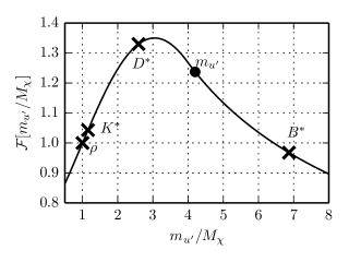
Figure 14: The normalized interpolating function ${\mathcal{F}}$ used to estimate the decay constant $f_{u^{\prime}}$ as a function of the dimensionless quantity $m_{u^{\prime}}/M_{\chi}$. The function ${\mathcal{F}}$ is chosen such that it reproduces the measured QCD decay constants $f_{\rho}$, $f_{K^{*}}$, $f_{D^{*}}$, $f_{B^{*}}$, denoted with crosses. The value of $m_{u^{\prime}}$ used in the benchmark is denoted by a circle.

Appendix C Decay widths

The decay widths for $\rho$ and $K^{*}$ decays to pseudoscalar pairs are given by

$$\begin{split}{\Gamma_{\rho}\over m_{\rho}}&={1\over 96\pi}\bigg{[}2g_{\rho\pi\pi}^{2}\left(1-{4m_{\pi}^{2}\over m_{\rho}^{2}}\right)^{3/2}\\ &\qquad\qquad+g^{2}_{\rho KK}\left(1-{4m_{K}^{2}\over m_{\rho}^{2}}\right)^{3/2}\bigg{]},\\ {\Gamma_{K^{*}}\over m_{K^{*}}}&={g_{K^{*}K\pi}^{2}\over 64\pi}\left[f_{\rm PS}\left(\tfrac{m_{\pi}}{m_{K^{*}}},\tfrac{m_{K}}{m_{K^{*}}}\right)\right]^{3}\\ &\quad+\,{g_{K^{*}K\eta_{8}}^{2}\over 64\pi}\left[f_{\rm PS}\left(\tfrac{m_{\eta_{8}}}{m_{K^{*}}},\tfrac{m_{K}}{m_{K^{*}}}\right)\right]^{3}.\end{split}$$ (90)

Here the phase-space function is defined as

$$f_{\rm PS}(x,y)=1-2x^{2}-2y^{2}\,.$$ (91)

Note that, due to flavor-symmetry breaking, the effective couplings $g_{\rho KK}$, $g_{K^{*}K\pi}$, $g_{K^{*}K\eta_{8}}$ could differ from $g_{\rho\pi\pi}$, defined in the flavor-symmetric limit in Eq. (14). In our numerics we take, however, all of them equal to the VMD value $g_{\rho}$, as discussed in Section II.2.

The decay widths of $V_{L}$ and $V_{H}$ read:

$$\begin{split}{\Gamma_{V_{L}}\over m_{V_{L}}}={g_{\rho}^{2}\over 32\pi}\sin^{2}\theta_{V}\left(1-4{m_{K}^{2}\over m_{V_{L}}^{2}}\right)^{3/2}&\,,\\ {\Gamma_{V_{H}}\over m_{V_{H}}}={g_{\rho}^{2}\over 32\pi}\cos^{2}\theta_{V}\left(1-4{m_{K}^{2}\over m_{V_{H}}^{2}}\right)^{3/2}&\,,\end{split}$$ (92)

where $\theta_{V}$ is the mixing angle in Eq. (75), and we have used the VMD estimate of the effective coupling.

The partial widths of the vector mesons to SM quarks are governed by their mixing with the would-be composite quarks, see Eq. (33). For instance, the $\bar{K}^{*1}\to\bar{t}u$ partial decay width is given by

$$\frac{\Gamma_{\bar{K}^{*1}\to\bar{t}u}}{M_{K^{*}}} =\frac{1}{16\pi}f_{\rm PS}\bigg{(}0,\frac{m_{t}}{m_{K^{*}}}\bigg{)}\Big{[}\big{(}\lambda_{13}^{R}\big{)}^{2}+\big{(}\lambda_{13}^{L}\big{)}^{2}\Big{]}$$

$$\quad\times\left[1-\frac{m_{t}^{2}}{2m_{K^{*}}^{2}}-\frac{1}{2}\bigg{(}\frac{m_{t}^{2}}{m_{K^{*}}^{2}}\bigg{)}^{2}\right]\,,$$ (93)

and similarly for $\Gamma_{\bar{K}^{*2}\to\bar{t}c}$ with $\lambda_{13}^{L/R}\rightarrow\lambda_{23}^{L/R}$.

The ${}^{3}P_{1}$ axial vectors can have $A\to VP$ decays and, if kinematically allowed, $A\to VV$ decays. The former usually dominate. To estimate the corresponding decay widths we follow the phenomenological analysis for $A\to VP$ decays in QCD given in Ref. Roca et al. (2004), and carried out in the ${\rm SU}(3)$ limit. The authors point out that in general one can express the decay amplitudes in terms of two independent operators,

$$\langle A_{\mu\nu}[V^{\mu\nu},P]\rangle\,,~{}~{}~{}\langle A_{\mu}[V^{\mu},P]\rangle\,.$$ (94)

They only choose the first operator for their study, which involves the tensor representations for the vector operators. However, they explain that an analysis involving only the second operator would yield similar results. The $A\to VP$ Lagrangian, in the ${\rm SU}(3)$ limit, is then

$${\cal L}_{AVP}=i\tilde{F}\langle A_{\mu\nu}[V^{\mu\nu},P]\rangle\,,$$ (95)

where $\langle\dots\rangle$ denotes a trace over the ${\rm SU}(3)$ generators, $\tilde{F}$ is a dimensionful coupling, and the factor $i$ insures that the Lagrangian is Hermitian. The tensor-field operators $V_{\mu\nu}$ is normalized such that

$$\langle 0|V_{\mu\nu}|V(P,\epsilon)\rangle=\frac{i}{M_{V}}\left(P_{\mu}\,\epsilon_{\nu}-P_{\nu}\,\epsilon_{\mu}\right),$$ (96)

and similarly for $A_{\mu\nu}$.

The partial decay widths of the axial vectors are then given by

$$\Gamma_{A\to VP}=\frac{|\lambda_{AVP}|^{2}}{2\pi}\frac{\tilde{F}^{2}q}{m_{A}^{2}}\left(1+\frac{2}{3}\frac{q^{2}}{m_{V}^{2}}\right),$$ (97)

where $q=f_{\rm PS}(m_{V}^{2}/m_{A}^{2},m_{P}^{2}/m_{A}^{2})\cdot 1/{(2m_{A})}$, and $\lambda_{AVP}$ are decay-mode-specific dimensionless prefactors. For instance, the mixed flavor octet-singlet states $A_{L}$ and $A_{H}$ decay to $K^{*}K$ final states. Summing over the $K^{*\pm}K^{\mp}$, $K^{*0}\bar{K}^{0}$, and $\bar{K}^{*0}K^{0}$ decay modes, the $A_{L}\to K^{*}K$ and $A_{H}\to K^{*}K$ decay widths are obtained by using the expression

$$\begin{split}\lambda_{A_{L,H}K^{*}K}=&2\Big{(}{\cos^{2}\theta_{\rm A}^{\rm id}\over 2}+\sin^{2}\theta_{\rm A}^{\rm id}\pm\sqrt{2}\sin\theta_{\rm A}^{\rm id}\cos\theta_{\rm A}^{\rm id}\Big{)}^{1/2},\\ \end{split}$$ (98)

for the $\lambda$ prefactor in Eq. (97)

The $a_{1}$ decays to $\rho\pi$ and $K^{*}K$. Summing over these final states, the $a_{1}\to\rho\pi$ and $a_{1}\to K^{*}K$ partial decay widths are obtained by using

$$\lambda_{a_{1}\rho\pi}=2\quad\text{and}\quad\lambda_{a_{1}K*K}=\sqrt{2}$$ (99)

in Eq. (97). The $K_{1}\to\rho K,K^{*}\pi,K\omega,K\phi$ partial decay widths follow from Eq. (97) using

$$\begin{split}\lambda_{K_{1}\rho K,K_{1}\pi K^{*}}&=\sqrt{3\over 2}\,,\quad\lambda_{K_{1}\omega K}={1\over\sqrt{2}}\,,\quad\lambda_{K_{1}\phi K}=1\,.\end{split}$$ (100)

The fits to the QCD axial-vector decay widths yield a large allowed range for $\tilde{F}$. In particular, the solutions for $\tilde{F}$ vary from $\tilde{F}_{\rm QCD}\approx 1200$ MeV to $\tilde{F}_{\rm QCD}\approx 1600$ MeV. We rescale from QCD with the usual scale factor,

$$\tilde{F}_{\rm HC}={M_{\chi}\over m_{\rho^{\rm QCD}}}\,\tilde{F}_{\rm QCD}\,.$$ (101)

Finally, we quote the total decay width of the heavy scalar ${\cal S}$, including the phase-space factors

$$\begin{split}\frac{\Gamma_{{\cal S}\to u_{i}\bar{\cal Q}_{i}}}{m_{\cal S}}=\frac{|h_{i}|^{2}}{16\pi}f_{\rm PS}\bigg{(}\frac{m_{u_{i}}}{m_{\cal S}}\,,\frac{m_{{\cal Q}_{i}}}{m_{\cal S}}\bigg{)}\biggl{(}1-\frac{m^{2}_{u_{i}}}{m_{\cal S}^{2}}-\frac{m_{{\cal Q}_{i}}^{2}}{m_{\cal S}^{2}}\biggl{)}\,.\end{split}$$ (102)

References

- Simmons (1989) E. H. Simmons, Nucl.Phys. B312, 253 (1989).
- Samuel (1990) S. Samuel, Nucl.Phys. B347, 625 (1990).
- Dine et al. (1990) M. Dine, A. Kagan, and S. Samuel, Phys.Lett. B243, 250 (1990).
- Carone and Simmons (1993) C. D. Carone and E. H. Simmons, Nucl.Phys. B397, 591 (1993), eprint hep-ph/9207273.
- Carone and Georgi (1994) C. D. Carone and H. Georgi, Phys.Rev. D49, 1427 (1994), eprint hep-ph/9308205.
- (6) A. L. Kagan, talk at 2008 KITP workshop on Physics of the Large Hadron Collider, http://online.itp.ucsb.edu/online/lhc08/kagan/.
- Antola et al. (2010) M. Antola, M. Heikinheimo, F. Sannino, and K. Tuominen, JHEP 1003, 050 (2010), eprint 0910.3681.
- Azatov et al. (2012a) A. Azatov, J. Galloway, and M. A. Luty, Phys.Rev.Lett. 108, 041802 (2012a), eprint 1106.3346.
- Azatov et al. (2012b) A. Azatov, J. Galloway, and M. A. Luty, Phys.Rev. D85, 015018 (2012b), eprint 1106.4815.
- Strassler and Zurek (2007) M. J. Strassler and K. M. Zurek, Phys.Lett. B651, 374 (2007), eprint hep-ph/0604261.
- Han et al. (2008) T. Han, Z. Si, K. M. Zurek, and M. J. Strassler, JHEP 0807, 008 (2008), eprint 0712.2041.
- Okun (1980a) L. Okun, JETP Lett. 31, 144 (1980a).
- Okun (1980b) L. Okun, Nucl.Phys. B173, 1 (1980b).
- Kang and Luty (2009) J. Kang and M. A. Luty, JHEP 0911, 065 (2009), eprint 0805.4642.
- Kribs et al. (2010) G. D. Kribs, T. S. Roy, J. Terning, and K. M. Zurek, Phys.Rev. D81, 095001 (2010), eprint 0909.2034.
- Burdman et al. (2008) G. Burdman, Z. Chacko, H.-S. Goh, R. Harnik, and C. A. Krenke, Phys.Rev. D78, 075028 (2008), eprint 0805.4667.
- Harnik and Wizansky (2009) R. Harnik and T. Wizansky, Phys.Rev. D80, 075015 (2009), eprint 0810.3948.
- Martin (2011) S. P. Martin, Phys.Rev. D83, 035019 (2011), eprint 1012.2072.
- Kilic et al. (2008) C. Kilic, T. Okui, and R. Sundrum, JHEP 0807, 038 (2008), eprint 0802.2568.
- Kilic et al. (2009) C. Kilic, S. Schumann, and M. Son, JHEP 0904, 128 (2009), eprint 0810.5542.
- Kilic et al. (2010) C. Kilic, T. Okui, and R. Sundrum, JHEP 1002, 018 (2010), eprint 0906.0577.
- Kilic and Okui (2010) C. Kilic and T. Okui, JHEP 1004, 128 (2010), eprint 1001.4526.
- Kamenik et al. (2012) J. F. Kamenik, J. Shu, and J. Zupan, Eur.Phys.J. C72, 2102 (2012), eprint 1107.5257.
- Grinstein et al. (2011a) B. Grinstein, A. L. Kagan, M. Trott, and J. Zupan, Phys.Rev.Lett. 107, 012002 (2011a), eprint 1102.3374.
- Grinstein et al. (2011b) B. Grinstein, A. L. Kagan, J. Zupan, and M. Trott, JHEP 1110, 072 (2011b), eprint 1108.4027.
- Gresham et al. (2012a) M. I. Gresham, I.-W. Kim, and K. M. Zurek, Phys.Rev. D85, 014022 (2012a), eprint 1107.4364.
- Grinstein et al. (2010) B. Grinstein, M. Redi, and G. Villadoro, JHEP 1011, 067 (2010), eprint 1009.2049.
- Ko et al. (2012) P. Ko, Y. Omura, and C. Yu, Phys.Rev. D85, 115010 (2012), eprint 1108.0350.
- Jung et al. (2010) S. Jung, H. Murayama, A. Pierce, and J. D. Wells, Phys.Rev. D81, 015004 (2010), eprint 0907.4112.
- Cui et al. (2011) Y. Cui, Z. Han, and M. D. Schwartz, JHEP 1107, 127 (2011), eprint 1106.3086.
- Blum et al. (2011) K. Blum, Y. Hochberg, and Y. Nir, JHEP 1110, 124 (2011), eprint 1107.4350.
- Drobnak et al. (2012) J. Drobnak, A. L. Kagan, J. F. Kamenik, G. Perez, and J. Zupan, Phys.Rev. D86, 094040 (2012), eprint 1209.4872.
- Grossman et al. (2007) Y. Grossman, Y. Nir, J. Thaler, T. Volansky, and J. Zupan, Phys.Rev. D76, 096006 (2007), eprint 0706.1845.
- McNeile et al. (2013) C. McNeile, A. Bazavov, C. Davies, R. Dowdall, K. Hornbostel, et al., Phys.Rev. D87, 034503 (2013), eprint 1211.6577.
- Beneke et al. (2007) M. Beneke, J. Rohrer, and D. Yang, Nucl.Phys. B774, 64 (2007), eprint hep-ph/0612290.
- Yang (2007) K.-C. Yang, Nucl.Phys. B776, 187 (2007), eprint 0705.0692.
- Isgur et al. (1989) N. Isgur, C. Morningstar, and C. Reader, Phys.Rev. D39, 1357 (1989).
- Beringer et al. (2012) J. Beringer et al. (Particle Data Group), Phys.Rev. D86, 010001 (2012).
- Cheng and Shrock (2011) H.-Y. Cheng and R. Shrock, Phys.Rev. D84, 094008 (2011), eprint 1109.3877.
- Roca et al. (2004) L. Roca, J. Palomar, and E. Oset, Phys.Rev. D70, 094006 (2004), eprint hep-ph/0306188.
- Abada et al. (2004) A. Abada, D. Becirevic, P. Boucaud, G. Herdoiza, J. Leroy, et al., JHEP 0402, 016 (2004), eprint hep-lat/0310050.
- Ohki et al. (2008) H. Ohki, H. Matsufuru, and T. Onogi, Phys.Rev. D77, 094509 (2008), eprint 0802.1563.
- El-Bennich et al. (2011) B. El-Bennich, M. A. Ivanov, and C. D. Roberts, Phys.Rev. C83, 025205 (2011), eprint 1012.5034.
- Kuhn and Rodrigo (1998) J. H. Kuhn and G. Rodrigo, Phys.Rev.Lett. 81, 49 (1998), eprint hep-ph/9802268.
- Kuhn and Rodrigo (1999) J. H. Kuhn and G. Rodrigo, Phys.Rev. D59, 054017 (1999), eprint hep-ph/9807420.
- Kuhn and Rodrigo (2012) J. H. Kuhn and G. Rodrigo, JHEP 1201, 063 (2012), eprint 1109.6830.
- Ahrens et al. (2011) V. Ahrens, A. Ferroglia, M. Neubert, B. D. Pecjak, and L. L. Yang, Phys.Rev. D84, 074004 (2011), eprint 1106.6051.
- Manohar and Trott (2012) A. V. Manohar and M. Trott, Phys.Lett. B711, 313 (2012), eprint 1201.3926.
- Hollik and Pagani (2011) W. Hollik and D. Pagani, Phys.Rev. D84, 093003 (2011), eprint 1107.2606.