Adiabatic quantum optimization in presence of discrete noise: Reducing the problem dimensionality

Salvatore Mandrà    Gian Giacomo Guerreschi    Alán Aspuru-Guzik Department of Chemistry and Chemical Biology, Harvard University, 12 Oxford Street, 02138 Cambridge MA
Abstract

Adiabatic quantum optimization is a procedure to solve a vast class of optimization problems by slowly changing the Hamiltonian of a quantum system. The evolution time necessary for the algorithm to be successful scales inversely with the minimum energy gap encountered during the dynamics. Unfortunately, the direct calculation of the gap is strongly limited by the exponential growth in the dimensionality of the Hilbert space associated to the quantum system. Although many special-purpose methods have been devised to reduce the effective dimensionality, they are strongly limited to particular classes of problems with evident symmetries. Moreover, little is known about the computational power of adiabatic quantum optimizers in real-world conditions. Here, we propose and implement a general purposes reduction method that does not rely on any explicit symmetry and which requires, under certain general conditions, only a polynomial amount of classical resources. Thanks to this method, we are able to analyze the performance of “non-ideal” quantum adiabatic optimizers to solve the well-known Grover problem, namely the search of target entries in an unsorted database, in the presence of discrete local defects. In this case, we show that adiabatic quantum optimization, even if affected by random noise, is still potentially faster than any classical algorithm.

I Introduction

In 2001, Farhi et al. Farhi2001a proposed a new paradigm to carry out quantum computation (QC) that is based on the adiabatic evolution of a quantum system under a slowly changing Hamiltonian and that builds on previous results developed by the statistical and chemical physics communities in the context of quantum annealing techniques Ray1989 ; Kadowaki1998 ; Finnila1994 ; Lee2000 . While this approach constitutes an alternative framework in which the development of new quantum algorithms for optimization problems results more intuitive Babbush2012 ; somma2012quantum ; perdomo2012finding , the estimation of the evolution time and its scaling with the problem size still remains unclear. For example, factors like the choice of the schedule Roland2002 ; Farhi2002 and the specific form of the Hamiltonian Das2002 ; Wei2006 ; altshuler2010anderson ; Choi2011 influence the adiabatic evolution in ways that are, so far, not fully understood. Adiabatic QC at zero temperature has been proved to be polynomially equivalent to the usual QC with gates and circuits vanDam2001 ; Aharonov2008 and, therefore, any exponential quantum speedup should be attainable Deutsch1992 ; Grover1996 ; Shor1999 ; Abrams1999 . In this respect, several numerical studies carried out in the last few years reported encouraging results for small systems Farhi2001a ; Hogg2003 ; Perdomo-Ortiz2010 ; Choi2011 ; hen2012solving ; Crosson2014 , exactly solvable systems somma2012quantum ; Roland2002 , and specific quantum chemistry or state preparation problems aspuru2005simulated ; yung2014transistor ; mcclean2013feynman ; peruzzo2013variational . In contrast, recent results in the context of experimental quantum annealing machines, which operate according to the same principle of adiabatic QC but in a thermal environment, showed no evidence of quantum speedup for random optimization problems Ronnow2014 .

To shed light on the actual power of QC, it is of great importance to be able to perform extensive numerical and theoretical studies on large quantum systems. Unfortunately, these kinds of analyses are strongly limited by the exponential growth in dimensionality of quantum systems. In the context of adiabatic QC, the evolution time, and thus the computational effort it quantifies, is related to the minimum energy gap between the ground state and the first excited state along the quantum evolution. The direct calculation of the energy gap is feasible only for optimization problems up to $n\approx 30$ qubits Farhi2001a ; Hogg2003 ; Perdomo-Ortiz2010 ; Crosson2014 . Estimations through quantum Monte Carlo techniques work only at finite temperature and require a large overhead due to the equilibration and evolution steps necessary to describe the situation at every stage of the adiabatic process santoro2002theory ; battaglia2006optimization ; Young2008 ; hen2012excitation .

Driver Hamiltonian Problem Hamiltonian Dimensionality
Grover Problem
HD(G)superscriptsubscript𝐻𝐷𝐺\leavevmode\hbox to15.21pt{\vbox to19.48pt{\pgfpicture\makeatletter\hbox{\hskip 9.02347pt\lower-4.76773pt\hbox to0.0pt{\pgfsys@beginscope\pgfsys@invoke{ }\definecolor{pgfstrokecolor}{rgb}{0,0,0}\pgfsys@color@rgb@stroke{0}{0}{0}\pgfsys@invoke{ }\pgfsys@color@rgb@fill{0}{0}{0}\pgfsys@invoke{ }\pgfsys@setlinewidth{0.4pt}\pgfsys@invoke{ }\nullfont\hbox to0.0pt{\pgfsys@beginscope\pgfsys@invoke{ }{}{}{}{{}}{}{{}{}}{{}}{} {}{{}}{}{}{}{}{{}}{}{{}}\pgfsys@beginscope\pgfsys@invoke{ }\pgfsys@setlinewidth{1.0pt}\pgfsys@invoke{ }\definecolor{pgffillcolor}{rgb}{1,0.9,0.9}\pgfsys@color@rgb@fill{1}{0.9}{0.9}\pgfsys@invoke{ }\definecolor{pgfstrokecolor}{rgb}{1,0.7,0.7}\pgfsys@color@rgb@stroke{1}{0.7}{0.7}\pgfsys@invoke{ }{{}{}{{}}}{{}{}{{}}}{}{}{{}{}{{}}}{{}{}{{}}}{}{}{{}{}{{}}}{{}{}{{}}}{}{}{{}{}{{}}}{{}{}{{}}}{}{}{}\pgfsys@moveto{0.0pt}{0.0pt}\pgfsys@moveto{5.69046pt}{-4.26773pt}\pgfsys@moveto{5.69046pt}{-0.26773pt}\pgfsys@lineto{5.69046pt}{7.38092pt}\pgfsys@curveto{5.69046pt}{9.59009pt}{3.89963pt}{11.38092pt}{1.69046pt}{11.38092pt}\pgfsys@lineto{-1.69046pt}{11.38092pt}\pgfsys@curveto{-3.89963pt}{11.38092pt}{-5.69046pt}{9.59009pt}{-5.69046pt}{7.38092pt}\pgfsys@lineto{-5.69046pt}{-0.26773pt}\pgfsys@curveto{-5.69046pt}{-2.4769pt}{-3.89963pt}{-4.26773pt}{-1.69046pt}{-4.26773pt}\pgfsys@lineto{1.69046pt}{-4.26773pt}\pgfsys@curveto{3.89963pt}{-4.26773pt}{5.69046pt}{-2.4769pt}{5.69046pt}{-0.26773pt}\pgfsys@closepath\pgfsys@moveto{-5.69046pt}{11.38092pt}\pgfsys@fillstroke\pgfsys@invoke{ }\hbox{\hbox{{\pgfsys@beginscope\pgfsys@invoke{ }{{}{}{{ {}{}}}{ {}{}} {{}{{}}}{{}{}}{}{{}{}}{}{}{}{}{} { }{{{{}}\pgfsys@beginscope\pgfsys@invoke{ }\pgfsys@transformcm{1.0}{0.0}{0.0}{1.0}{-5.69046pt}{11.38092pt}\pgfsys@invoke{ }\hbox{{\definecolor{pgfstrokecolor}{rgb}{0,0,0}\pgfsys@color@rgb@stroke{0}{0}{0}\pgfsys@invoke{ }\pgfsys@color@rgb@fill{0}{0}{0}\pgfsys@invoke{ }\hbox{} }}\pgfsys@invoke{\lxSVG@closescope }\pgfsys@endscope}}} \pgfsys@invoke{\lxSVG@closescope }\pgfsys@endscope}}} \pgfsys@invoke{\lxSVG@closescope }\pgfsys@endscope \pgfsys@invoke{\lxSVG@closescope }\pgfsys@endscope\hbox to0.0pt{}{}{}{}\hss}\pgfsys@discardpath\pgfsys@invoke{\lxSVG@closescope }\pgfsys@endscope\hss}}\lxSVG@closescope\endpgfpicture}}H_{D}^{(G)}\leavevmode\hbox to0pt{\vbox to0pt{\pgfpicture\makeatletter\hbox{\hskip 0.0pt\lower 0.0pt\hbox to0.0pt{\pgfsys@beginscope\pgfsys@invoke{ }\definecolor{pgfstrokecolor}{rgb}{0,0,0}\pgfsys@color@rgb@stroke{0}{0}{0}\pgfsys@invoke{ }\pgfsys@color@rgb@fill{0}{0}{0}\pgfsys@invoke{ }\pgfsys@setlinewidth{0.4pt}\pgfsys@invoke{ }\nullfont\hbox to0.0pt{\pgfsys@beginscope\pgfsys@invoke{ }\immediate; \pgfsys@invoke{\lxSVG@closescope }\pgfsys@endscope\hbox to0.0pt{}{}{}{}\hss}\pgfsys@discardpath\pgfsys@invoke{\lxSVG@closescope }\pgfsys@endscope\hss}}\lxSVG@closescope\endpgfpicture}} |σσ|ketsuperscript𝜎brasuperscript𝜎\leavevmode\hbox to15.21pt{\vbox to19.48pt{\pgfpicture\makeatletter\hbox{\hskip 9.02347pt\lower-4.76773pt\hbox to0.0pt{\pgfsys@beginscope\pgfsys@invoke{ }\definecolor{pgfstrokecolor}{rgb}{0,0,0}\pgfsys@color@rgb@stroke{0}{0}{0}\pgfsys@invoke{ }\pgfsys@color@rgb@fill{0}{0}{0}\pgfsys@invoke{ }\pgfsys@setlinewidth{0.4pt}\pgfsys@invoke{ }\nullfont\hbox to0.0pt{\pgfsys@beginscope\pgfsys@invoke{ }{}{}{}{{}}{}{{}{}}{{}}{} {}{{}}{}{}{}{}{{}}{}{{}}\pgfsys@beginscope\pgfsys@invoke{ }\pgfsys@setlinewidth{1.0pt}\pgfsys@invoke{ }\definecolor{pgffillcolor}{rgb}{0.9,0.9,1}\pgfsys@color@rgb@fill{0.9}{0.9}{1}\pgfsys@invoke{ }\definecolor{pgfstrokecolor}{rgb}{0.7,0.7,1}\pgfsys@color@rgb@stroke{0.7}{0.7}{1}\pgfsys@invoke{ }{{}{}{{}}}{{}{}{{}}}{}{}{{}{}{{}}}{{}{}{{}}}{}{}{{}{}{{}}}{{}{}{{}}}{}{}{{}{}{{}}}{{}{}{{}}}{}{}{}\pgfsys@moveto{0.0pt}{0.0pt}\pgfsys@moveto{5.69046pt}{-4.26773pt}\pgfsys@moveto{5.69046pt}{-0.26773pt}\pgfsys@lineto{5.69046pt}{7.38092pt}\pgfsys@curveto{5.69046pt}{9.59009pt}{3.89963pt}{11.38092pt}{1.69046pt}{11.38092pt}\pgfsys@lineto{-1.69046pt}{11.38092pt}\pgfsys@curveto{-3.89963pt}{11.38092pt}{-5.69046pt}{9.59009pt}{-5.69046pt}{7.38092pt}\pgfsys@lineto{-5.69046pt}{-0.26773pt}\pgfsys@curveto{-5.69046pt}{-2.4769pt}{-3.89963pt}{-4.26773pt}{-1.69046pt}{-4.26773pt}\pgfsys@lineto{1.69046pt}{-4.26773pt}\pgfsys@curveto{3.89963pt}{-4.26773pt}{5.69046pt}{-2.4769pt}{5.69046pt}{-0.26773pt}\pgfsys@closepath\pgfsys@moveto{-5.69046pt}{11.38092pt}\pgfsys@fillstroke\pgfsys@invoke{ }\hbox{\hbox{{\pgfsys@beginscope\pgfsys@invoke{ }{{}{}{{ {}{}}}{ {}{}} {{}{{}}}{{}{}}{}{{}{}}{}{}{}{}{} { }{{{{}}\pgfsys@beginscope\pgfsys@invoke{ }\pgfsys@transformcm{1.0}{0.0}{0.0}{1.0}{-5.69046pt}{11.38092pt}\pgfsys@invoke{ }\hbox{{\definecolor{pgfstrokecolor}{rgb}{0,0,0}\pgfsys@color@rgb@stroke{0}{0}{0}\pgfsys@invoke{ }\pgfsys@color@rgb@fill{0}{0}{0}\pgfsys@invoke{ }\hbox{} }}\pgfsys@invoke{\lxSVG@closescope }\pgfsys@endscope}}} \pgfsys@invoke{\lxSVG@closescope }\pgfsys@endscope}}} \pgfsys@invoke{\lxSVG@closescope }\pgfsys@endscope \pgfsys@invoke{\lxSVG@closescope }\pgfsys@endscope\hbox to0.0pt{}{}{}{}\hss}\pgfsys@discardpath\pgfsys@invoke{\lxSVG@closescope }\pgfsys@endscope\hss}}\lxSVG@closescope\endpgfpicture}}-\Ket{\sigma^{*}}\!\!\Bra{\sigma^{*}}\leavevmode\hbox to0pt{\vbox to0pt{\pgfpicture\makeatletter\hbox{\hskip 0.0pt\lower 0.0pt\hbox to0.0pt{\pgfsys@beginscope\pgfsys@invoke{ }\definecolor{pgfstrokecolor}{rgb}{0,0,0}\pgfsys@color@rgb@stroke{0}{0}{0}\pgfsys@invoke{ }\pgfsys@color@rgb@fill{0}{0}{0}\pgfsys@invoke{ }\pgfsys@setlinewidth{0.4pt}\pgfsys@invoke{ }\nullfont\hbox to0.0pt{\pgfsys@beginscope\pgfsys@invoke{ }\immediate; \pgfsys@invoke{\lxSVG@closescope }\pgfsys@endscope\hbox to0.0pt{}{}{}{}\hss}\pgfsys@discardpath\pgfsys@invoke{\lxSVG@closescope }\pgfsys@endscope\hss}}\lxSVG@closescope\endpgfpicture}} 2
Grover Problem
HD(S)superscriptsubscript𝐻𝐷𝑆\leavevmode\hbox to15.21pt{\vbox to19.48pt{\pgfpicture\makeatletter\hbox{\hskip 9.02347pt\lower-4.76773pt\hbox to0.0pt{\pgfsys@beginscope\pgfsys@invoke{ }\definecolor{pgfstrokecolor}{rgb}{0,0,0}\pgfsys@color@rgb@stroke{0}{0}{0}\pgfsys@invoke{ }\pgfsys@color@rgb@fill{0}{0}{0}\pgfsys@invoke{ }\pgfsys@setlinewidth{0.4pt}\pgfsys@invoke{ }\nullfont\hbox to0.0pt{\pgfsys@beginscope\pgfsys@invoke{ }{}{}{}{{}}{}{{}{}}{{}}{} {}{{}}{}{}{}{}{{}}{}{{}}\pgfsys@beginscope\pgfsys@invoke{ }\pgfsys@setlinewidth{1.0pt}\pgfsys@invoke{ }\definecolor{pgffillcolor}{rgb}{1,0.9,0.9}\pgfsys@color@rgb@fill{1}{0.9}{0.9}\pgfsys@invoke{ }\definecolor{pgfstrokecolor}{rgb}{1,0.7,0.7}\pgfsys@color@rgb@stroke{1}{0.7}{0.7}\pgfsys@invoke{ }{{}{}{{}}}{{}{}{{}}}{}{}{{}{}{{}}}{{}{}{{}}}{}{}{{}{}{{}}}{{}{}{{}}}{}{}{{}{}{{}}}{{}{}{{}}}{}{}{}\pgfsys@moveto{0.0pt}{0.0pt}\pgfsys@moveto{5.69046pt}{-4.26773pt}\pgfsys@moveto{5.69046pt}{-0.26773pt}\pgfsys@lineto{5.69046pt}{7.38092pt}\pgfsys@curveto{5.69046pt}{9.59009pt}{3.89963pt}{11.38092pt}{1.69046pt}{11.38092pt}\pgfsys@lineto{-1.69046pt}{11.38092pt}\pgfsys@curveto{-3.89963pt}{11.38092pt}{-5.69046pt}{9.59009pt}{-5.69046pt}{7.38092pt}\pgfsys@lineto{-5.69046pt}{-0.26773pt}\pgfsys@curveto{-5.69046pt}{-2.4769pt}{-3.89963pt}{-4.26773pt}{-1.69046pt}{-4.26773pt}\pgfsys@lineto{1.69046pt}{-4.26773pt}\pgfsys@curveto{3.89963pt}{-4.26773pt}{5.69046pt}{-2.4769pt}{5.69046pt}{-0.26773pt}\pgfsys@closepath\pgfsys@moveto{-5.69046pt}{11.38092pt}\pgfsys@fillstroke\pgfsys@invoke{ }\hbox{\hbox{{\pgfsys@beginscope\pgfsys@invoke{ }{{}{}{{ {}{}}}{ {}{}} {{}{{}}}{{}{}}{}{{}{}}{}{}{}{}{} { }{{{{}}\pgfsys@beginscope\pgfsys@invoke{ }\pgfsys@transformcm{1.0}{0.0}{0.0}{1.0}{-5.69046pt}{11.38092pt}\pgfsys@invoke{ }\hbox{{\definecolor{pgfstrokecolor}{rgb}{0,0,0}\pgfsys@color@rgb@stroke{0}{0}{0}\pgfsys@invoke{ }\pgfsys@color@rgb@fill{0}{0}{0}\pgfsys@invoke{ }\hbox{} }}\pgfsys@invoke{\lxSVG@closescope }\pgfsys@endscope}}} \pgfsys@invoke{\lxSVG@closescope }\pgfsys@endscope}}} \pgfsys@invoke{\lxSVG@closescope }\pgfsys@endscope \pgfsys@invoke{\lxSVG@closescope }\pgfsys@endscope\hbox to0.0pt{}{}{}{}\hss}\pgfsys@discardpath\pgfsys@invoke{\lxSVG@closescope }\pgfsys@endscope\hss}}\lxSVG@closescope\endpgfpicture}}H_{D}^{(S)}\leavevmode\hbox to0pt{\vbox to0pt{\pgfpicture\makeatletter\hbox{\hskip 0.0pt\lower 0.0pt\hbox to0.0pt{\pgfsys@beginscope\pgfsys@invoke{ }\definecolor{pgfstrokecolor}{rgb}{0,0,0}\pgfsys@color@rgb@stroke{0}{0}{0}\pgfsys@invoke{ }\pgfsys@color@rgb@fill{0}{0}{0}\pgfsys@invoke{ }\pgfsys@setlinewidth{0.4pt}\pgfsys@invoke{ }\nullfont\hbox to0.0pt{\pgfsys@beginscope\pgfsys@invoke{ }\immediate; \pgfsys@invoke{\lxSVG@closescope }\pgfsys@endscope\hbox to0.0pt{}{}{}{}\hss}\pgfsys@discardpath\pgfsys@invoke{\lxSVG@closescope }\pgfsys@endscope\hss}}\lxSVG@closescope\endpgfpicture}} |σσ|ketsuperscript𝜎brasuperscript𝜎\leavevmode\hbox to15.21pt{\vbox to19.48pt{\pgfpicture\makeatletter\hbox{\hskip 9.02347pt\lower-4.76773pt\hbox to0.0pt{\pgfsys@beginscope\pgfsys@invoke{ }\definecolor{pgfstrokecolor}{rgb}{0,0,0}\pgfsys@color@rgb@stroke{0}{0}{0}\pgfsys@invoke{ }\pgfsys@color@rgb@fill{0}{0}{0}\pgfsys@invoke{ }\pgfsys@setlinewidth{0.4pt}\pgfsys@invoke{ }\nullfont\hbox to0.0pt{\pgfsys@beginscope\pgfsys@invoke{ }{}{}{}{{}}{}{{}{}}{{}}{} {}{{}}{}{}{}{}{{}}{}{{}}\pgfsys@beginscope\pgfsys@invoke{ }\pgfsys@setlinewidth{1.0pt}\pgfsys@invoke{ }\definecolor{pgffillcolor}{rgb}{0.9,0.9,1}\pgfsys@color@rgb@fill{0.9}{0.9}{1}\pgfsys@invoke{ }\definecolor{pgfstrokecolor}{rgb}{0.7,0.7,1}\pgfsys@color@rgb@stroke{0.7}{0.7}{1}\pgfsys@invoke{ }{{}{}{{}}}{{}{}{{}}}{}{}{{}{}{{}}}{{}{}{{}}}{}{}{{}{}{{}}}{{}{}{{}}}{}{}{{}{}{{}}}{{}{}{{}}}{}{}{}\pgfsys@moveto{0.0pt}{0.0pt}\pgfsys@moveto{5.69046pt}{-4.26773pt}\pgfsys@moveto{5.69046pt}{-0.26773pt}\pgfsys@lineto{5.69046pt}{7.38092pt}\pgfsys@curveto{5.69046pt}{9.59009pt}{3.89963pt}{11.38092pt}{1.69046pt}{11.38092pt}\pgfsys@lineto{-1.69046pt}{11.38092pt}\pgfsys@curveto{-3.89963pt}{11.38092pt}{-5.69046pt}{9.59009pt}{-5.69046pt}{7.38092pt}\pgfsys@lineto{-5.69046pt}{-0.26773pt}\pgfsys@curveto{-5.69046pt}{-2.4769pt}{-3.89963pt}{-4.26773pt}{-1.69046pt}{-4.26773pt}\pgfsys@lineto{1.69046pt}{-4.26773pt}\pgfsys@curveto{3.89963pt}{-4.26773pt}{5.69046pt}{-2.4769pt}{5.69046pt}{-0.26773pt}\pgfsys@closepath\pgfsys@moveto{-5.69046pt}{11.38092pt}\pgfsys@fillstroke\pgfsys@invoke{ }\hbox{\hbox{{\pgfsys@beginscope\pgfsys@invoke{ }{{}{}{{ {}{}}}{ {}{}} {{}{{}}}{{}{}}{}{{}{}}{}{}{}{}{} { }{{{{}}\pgfsys@beginscope\pgfsys@invoke{ }\pgfsys@transformcm{1.0}{0.0}{0.0}{1.0}{-5.69046pt}{11.38092pt}\pgfsys@invoke{ }\hbox{{\definecolor{pgfstrokecolor}{rgb}{0,0,0}\pgfsys@color@rgb@stroke{0}{0}{0}\pgfsys@invoke{ }\pgfsys@color@rgb@fill{0}{0}{0}\pgfsys@invoke{ }\hbox{} }}\pgfsys@invoke{\lxSVG@closescope }\pgfsys@endscope}}} \pgfsys@invoke{\lxSVG@closescope }\pgfsys@endscope}}} \pgfsys@invoke{\lxSVG@closescope }\pgfsys@endscope \pgfsys@invoke{\lxSVG@closescope }\pgfsys@endscope\hbox to0.0pt{}{}{}{}\hss}\pgfsys@discardpath\pgfsys@invoke{\lxSVG@closescope }\pgfsys@endscope\hss}}\lxSVG@closescope\endpgfpicture}}-\Ket{\sigma^{*}}\!\!\Bra{\sigma^{*}}\leavevmode\hbox to0pt{\vbox to0pt{\pgfpicture\makeatletter\hbox{\hskip 0.0pt\lower 0.0pt\hbox to0.0pt{\pgfsys@beginscope\pgfsys@invoke{ }\definecolor{pgfstrokecolor}{rgb}{0,0,0}\pgfsys@color@rgb@stroke{0}{0}{0}\pgfsys@invoke{ }\pgfsys@color@rgb@fill{0}{0}{0}\pgfsys@invoke{ }\pgfsys@setlinewidth{0.4pt}\pgfsys@invoke{ }\nullfont\hbox to0.0pt{\pgfsys@beginscope\pgfsys@invoke{ }\immediate; \pgfsys@invoke{\lxSVG@closescope }\pgfsys@endscope\hbox to0.0pt{}{}{}{}\hss}\pgfsys@discardpath\pgfsys@invoke{\lxSVG@closescope }\pgfsys@endscope\hss}}\lxSVG@closescope\endpgfpicture}} n+1
Grover Problem with Many Solutions (see Appendix E)
HD(S)superscriptsubscript𝐻𝐷𝑆\leavevmode\hbox to15.21pt{\vbox to19.48pt{\pgfpicture\makeatletter\hbox{\hskip 9.02347pt\lower-4.76773pt\hbox to0.0pt{\pgfsys@beginscope\pgfsys@invoke{ }\definecolor{pgfstrokecolor}{rgb}{0,0,0}\pgfsys@color@rgb@stroke{0}{0}{0}\pgfsys@invoke{ }\pgfsys@color@rgb@fill{0}{0}{0}\pgfsys@invoke{ }\pgfsys@setlinewidth{0.4pt}\pgfsys@invoke{ }\nullfont\hbox to0.0pt{\pgfsys@beginscope\pgfsys@invoke{ }{}{}{}{{}}{}{{}{}}{{}}{} {}{{}}{}{}{}{}{{}}{}{{}}\pgfsys@beginscope\pgfsys@invoke{ }\pgfsys@setlinewidth{1.0pt}\pgfsys@invoke{ }\definecolor{pgffillcolor}{rgb}{1,0.9,0.9}\pgfsys@color@rgb@fill{1}{0.9}{0.9}\pgfsys@invoke{ }\definecolor{pgfstrokecolor}{rgb}{1,0.7,0.7}\pgfsys@color@rgb@stroke{1}{0.7}{0.7}\pgfsys@invoke{ }{{}{}{{}}}{{}{}{{}}}{}{}{{}{}{{}}}{{}{}{{}}}{}{}{{}{}{{}}}{{}{}{{}}}{}{}{{}{}{{}}}{{}{}{{}}}{}{}{}\pgfsys@moveto{0.0pt}{0.0pt}\pgfsys@moveto{5.69046pt}{-4.26773pt}\pgfsys@moveto{5.69046pt}{-0.26773pt}\pgfsys@lineto{5.69046pt}{7.38092pt}\pgfsys@curveto{5.69046pt}{9.59009pt}{3.89963pt}{11.38092pt}{1.69046pt}{11.38092pt}\pgfsys@lineto{-1.69046pt}{11.38092pt}\pgfsys@curveto{-3.89963pt}{11.38092pt}{-5.69046pt}{9.59009pt}{-5.69046pt}{7.38092pt}\pgfsys@lineto{-5.69046pt}{-0.26773pt}\pgfsys@curveto{-5.69046pt}{-2.4769pt}{-3.89963pt}{-4.26773pt}{-1.69046pt}{-4.26773pt}\pgfsys@lineto{1.69046pt}{-4.26773pt}\pgfsys@curveto{3.89963pt}{-4.26773pt}{5.69046pt}{-2.4769pt}{5.69046pt}{-0.26773pt}\pgfsys@closepath\pgfsys@moveto{-5.69046pt}{11.38092pt}\pgfsys@fillstroke\pgfsys@invoke{ }\hbox{\hbox{{\pgfsys@beginscope\pgfsys@invoke{ }{{}{}{{ {}{}}}{ {}{}} {{}{{}}}{{}{}}{}{{}{}}{}{}{}{}{} { }{{{{}}\pgfsys@beginscope\pgfsys@invoke{ }\pgfsys@transformcm{1.0}{0.0}{0.0}{1.0}{-5.69046pt}{11.38092pt}\pgfsys@invoke{ }\hbox{{\definecolor{pgfstrokecolor}{rgb}{0,0,0}\pgfsys@color@rgb@stroke{0}{0}{0}\pgfsys@invoke{ }\pgfsys@color@rgb@fill{0}{0}{0}\pgfsys@invoke{ }\hbox{} }}\pgfsys@invoke{\lxSVG@closescope }\pgfsys@endscope}}} \pgfsys@invoke{\lxSVG@closescope }\pgfsys@endscope}}} \pgfsys@invoke{\lxSVG@closescope }\pgfsys@endscope \pgfsys@invoke{\lxSVG@closescope }\pgfsys@endscope\hbox to0.0pt{}{}{}{}\hss}\pgfsys@discardpath\pgfsys@invoke{\lxSVG@closescope }\pgfsys@endscope\hss}}\lxSVG@closescope\endpgfpicture}}H_{D}^{(S)}\leavevmode\hbox to0pt{\vbox to0pt{\pgfpicture\makeatletter\hbox{\hskip 0.0pt\lower 0.0pt\hbox to0.0pt{\pgfsys@beginscope\pgfsys@invoke{ }\definecolor{pgfstrokecolor}{rgb}{0,0,0}\pgfsys@color@rgb@stroke{0}{0}{0}\pgfsys@invoke{ }\pgfsys@color@rgb@fill{0}{0}{0}\pgfsys@invoke{ }\pgfsys@setlinewidth{0.4pt}\pgfsys@invoke{ }\nullfont\hbox to0.0pt{\pgfsys@beginscope\pgfsys@invoke{ }\immediate; \pgfsys@invoke{\lxSVG@closescope }\pgfsys@endscope\hbox to0.0pt{}{}{}{}\hss}\pgfsys@discardpath\pgfsys@invoke{\lxSVG@closescope }\pgfsys@endscope\hss}}\lxSVG@closescope\endpgfpicture}} i=1p|σiσi|superscriptsubscript𝑖1𝑝ketsubscriptsuperscript𝜎𝑖brasubscriptsuperscript𝜎𝑖\leavevmode\hbox to15.21pt{\vbox to19.48pt{\pgfpicture\makeatletter\hbox{\hskip 9.02347pt\lower-4.76773pt\hbox to0.0pt{\pgfsys@beginscope\pgfsys@invoke{ }\definecolor{pgfstrokecolor}{rgb}{0,0,0}\pgfsys@color@rgb@stroke{0}{0}{0}\pgfsys@invoke{ }\pgfsys@color@rgb@fill{0}{0}{0}\pgfsys@invoke{ }\pgfsys@setlinewidth{0.4pt}\pgfsys@invoke{ }\nullfont\hbox to0.0pt{\pgfsys@beginscope\pgfsys@invoke{ }{}{}{}{{}}{}{{}{}}{{}}{} {}{{}}{}{}{}{}{{}}{}{{}}\pgfsys@beginscope\pgfsys@invoke{ }\pgfsys@setlinewidth{1.0pt}\pgfsys@invoke{ }\definecolor{pgffillcolor}{rgb}{0.9,0.9,1}\pgfsys@color@rgb@fill{0.9}{0.9}{1}\pgfsys@invoke{ }\definecolor{pgfstrokecolor}{rgb}{0.7,0.7,1}\pgfsys@color@rgb@stroke{0.7}{0.7}{1}\pgfsys@invoke{ }{{}{}{{}}}{{}{}{{}}}{}{}{{}{}{{}}}{{}{}{{}}}{}{}{{}{}{{}}}{{}{}{{}}}{}{}{{}{}{{}}}{{}{}{{}}}{}{}{}\pgfsys@moveto{0.0pt}{0.0pt}\pgfsys@moveto{5.69046pt}{-4.26773pt}\pgfsys@moveto{5.69046pt}{-0.26773pt}\pgfsys@lineto{5.69046pt}{7.38092pt}\pgfsys@curveto{5.69046pt}{9.59009pt}{3.89963pt}{11.38092pt}{1.69046pt}{11.38092pt}\pgfsys@lineto{-1.69046pt}{11.38092pt}\pgfsys@curveto{-3.89963pt}{11.38092pt}{-5.69046pt}{9.59009pt}{-5.69046pt}{7.38092pt}\pgfsys@lineto{-5.69046pt}{-0.26773pt}\pgfsys@curveto{-5.69046pt}{-2.4769pt}{-3.89963pt}{-4.26773pt}{-1.69046pt}{-4.26773pt}\pgfsys@lineto{1.69046pt}{-4.26773pt}\pgfsys@curveto{3.89963pt}{-4.26773pt}{5.69046pt}{-2.4769pt}{5.69046pt}{-0.26773pt}\pgfsys@closepath\pgfsys@moveto{-5.69046pt}{11.38092pt}\pgfsys@fillstroke\pgfsys@invoke{ }\hbox{\hbox{{\pgfsys@beginscope\pgfsys@invoke{ }{{}{}{{ {}{}}}{ {}{}} {{}{{}}}{{}{}}{}{{}{}}{}{}{}{}{} { }{{{{}}\pgfsys@beginscope\pgfsys@invoke{ }\pgfsys@transformcm{1.0}{0.0}{0.0}{1.0}{-5.69046pt}{11.38092pt}\pgfsys@invoke{ }\hbox{{\definecolor{pgfstrokecolor}{rgb}{0,0,0}\pgfsys@color@rgb@stroke{0}{0}{0}\pgfsys@invoke{ }\pgfsys@color@rgb@fill{0}{0}{0}\pgfsys@invoke{ }\hbox{} }}\pgfsys@invoke{\lxSVG@closescope }\pgfsys@endscope}}} \pgfsys@invoke{\lxSVG@closescope }\pgfsys@endscope}}} \pgfsys@invoke{\lxSVG@closescope }\pgfsys@endscope \pgfsys@invoke{\lxSVG@closescope }\pgfsys@endscope\hbox to0.0pt{}{}{}{}\hss}\pgfsys@discardpath\pgfsys@invoke{\lxSVG@closescope }\pgfsys@endscope\hss}}\lxSVG@closescope\endpgfpicture}}-\sum_{i=1}^{p}\Ket{\sigma^{*}_{i}}\!\!\Bra{\sigma^{*}_{i}}\leavevmode\hbox to0pt{\vbox to0pt{\pgfpicture\makeatletter\hbox{\hskip 0.0pt\lower 0.0pt\hbox to0.0pt{\pgfsys@beginscope\pgfsys@invoke{ }\definecolor{pgfstrokecolor}{rgb}{0,0,0}\pgfsys@color@rgb@stroke{0}{0}{0}\pgfsys@invoke{ }\pgfsys@color@rgb@fill{0}{0}{0}\pgfsys@invoke{ }\pgfsys@setlinewidth{0.4pt}\pgfsys@invoke{ }\nullfont\hbox to0.0pt{\pgfsys@beginscope\pgfsys@invoke{ }\immediate; \pgfsys@invoke{\lxSVG@closescope }\pgfsys@endscope\hbox to0.0pt{}{}{}{}\hss}\pgfsys@discardpath\pgfsys@invoke{\lxSVG@closescope }\pgfsys@endscope\hss}}\lxSVG@closescope\endpgfpicture}} $\leq$ p n
Grover Problem with local noise
HD(G)superscriptsubscript𝐻𝐷𝐺\leavevmode\hbox to15.21pt{\vbox to19.48pt{\pgfpicture\makeatletter\hbox{\hskip 9.02347pt\lower-4.76773pt\hbox to0.0pt{\pgfsys@beginscope\pgfsys@invoke{ }\definecolor{pgfstrokecolor}{rgb}{0,0,0}\pgfsys@color@rgb@stroke{0}{0}{0}\pgfsys@invoke{ }\pgfsys@color@rgb@fill{0}{0}{0}\pgfsys@invoke{ }\pgfsys@setlinewidth{0.4pt}\pgfsys@invoke{ }\nullfont\hbox to0.0pt{\pgfsys@beginscope\pgfsys@invoke{ }{}{}{}{{}}{}{{}{}}{{}}{} {}{{}}{}{}{}{}{{}}{}{{}}\pgfsys@beginscope\pgfsys@invoke{ }\pgfsys@setlinewidth{1.0pt}\pgfsys@invoke{ }\definecolor{pgffillcolor}{rgb}{0.9,0.9,1}\pgfsys@color@rgb@fill{0.9}{0.9}{1}\pgfsys@invoke{ }\definecolor{pgfstrokecolor}{rgb}{0.7,0.7,1}\pgfsys@color@rgb@stroke{0.7}{0.7}{1}\pgfsys@invoke{ }{{}{}{{}}}{{}{}{{}}}{}{}{{}{}{{}}}{{}{}{{}}}{}{}{{}{}{{}}}{{}{}{{}}}{}{}{{}{}{{}}}{{}{}{{}}}{}{}{}\pgfsys@moveto{0.0pt}{0.0pt}\pgfsys@moveto{5.69046pt}{-4.26773pt}\pgfsys@moveto{5.69046pt}{-0.26773pt}\pgfsys@lineto{5.69046pt}{7.38092pt}\pgfsys@curveto{5.69046pt}{9.59009pt}{3.89963pt}{11.38092pt}{1.69046pt}{11.38092pt}\pgfsys@lineto{-1.69046pt}{11.38092pt}\pgfsys@curveto{-3.89963pt}{11.38092pt}{-5.69046pt}{9.59009pt}{-5.69046pt}{7.38092pt}\pgfsys@lineto{-5.69046pt}{-0.26773pt}\pgfsys@curveto{-5.69046pt}{-2.4769pt}{-3.89963pt}{-4.26773pt}{-1.69046pt}{-4.26773pt}\pgfsys@lineto{1.69046pt}{-4.26773pt}\pgfsys@curveto{3.89963pt}{-4.26773pt}{5.69046pt}{-2.4769pt}{5.69046pt}{-0.26773pt}\pgfsys@closepath\pgfsys@moveto{-5.69046pt}{11.38092pt}\pgfsys@fillstroke\pgfsys@invoke{ }\hbox{\hbox{{\pgfsys@beginscope\pgfsys@invoke{ }{{}{}{{ {}{}}}{ {}{}} {{}{{}}}{{}{}}{}{{}{}}{}{}{}{}{} { }{{{{}}\pgfsys@beginscope\pgfsys@invoke{ }\pgfsys@transformcm{1.0}{0.0}{0.0}{1.0}{-5.69046pt}{11.38092pt}\pgfsys@invoke{ }\hbox{{\definecolor{pgfstrokecolor}{rgb}{0,0,0}\pgfsys@color@rgb@stroke{0}{0}{0}\pgfsys@invoke{ }\pgfsys@color@rgb@fill{0}{0}{0}\pgfsys@invoke{ }\hbox{} }}\pgfsys@invoke{\lxSVG@closescope }\pgfsys@endscope}}} \pgfsys@invoke{\lxSVG@closescope }\pgfsys@endscope}}} \pgfsys@invoke{\lxSVG@closescope }\pgfsys@endscope \pgfsys@invoke{\lxSVG@closescope }\pgfsys@endscope\hbox to0.0pt{}{}{}{}\hss}\pgfsys@discardpath\pgfsys@invoke{\lxSVG@closescope }\pgfsys@endscope\hss}}\lxSVG@closescope\endpgfpicture}}H_{D}^{(G)}\leavevmode\hbox to0pt{\vbox to0pt{\pgfpicture\makeatletter\hbox{\hskip 0.0pt\lower 0.0pt\hbox to0.0pt{\pgfsys@beginscope\pgfsys@invoke{ }\definecolor{pgfstrokecolor}{rgb}{0,0,0}\pgfsys@color@rgb@stroke{0}{0}{0}\pgfsys@invoke{ }\pgfsys@color@rgb@fill{0}{0}{0}\pgfsys@invoke{ }\pgfsys@setlinewidth{0.4pt}\pgfsys@invoke{ }\nullfont\hbox to0.0pt{\pgfsys@beginscope\pgfsys@invoke{ }\immediate; \pgfsys@invoke{\lxSVG@closescope }\pgfsys@endscope\hbox to0.0pt{}{}{}{}\hss}\pgfsys@discardpath\pgfsys@invoke{\lxSVG@closescope }\pgfsys@endscope\hss}}\lxSVG@closescope\endpgfpicture}} |σσ|ketsuperscript𝜎brasuperscript𝜎\leavevmode\hbox to9.52pt{\vbox to18.91pt{\pgfpicture\makeatletter\hbox{\hskip 6.17845pt\lower-5.62128pt\hbox to0.0pt{\pgfsys@beginscope\pgfsys@invoke{ }\definecolor{pgfstrokecolor}{rgb}{0,0,0}\pgfsys@color@rgb@stroke{0}{0}{0}\pgfsys@invoke{ }\pgfsys@color@rgb@fill{0}{0}{0}\pgfsys@invoke{ }\pgfsys@setlinewidth{0.4pt}\pgfsys@invoke{ }\nullfont\hbox to0.0pt{\pgfsys@beginscope\pgfsys@invoke{ }{}{}{}{{}}{}{{}{}}{{}}{} {}{{}}{}{}{}{}{{}}{}{{}}\pgfsys@beginscope\pgfsys@invoke{ }\pgfsys@setlinewidth{1.0pt}\pgfsys@invoke{ }\definecolor{pgffillcolor}{rgb}{0.9,0.9,1}\pgfsys@color@rgb@fill{0.9}{0.9}{1}\pgfsys@invoke{ }\definecolor{pgfstrokecolor}{rgb}{0.7,0.7,1}\pgfsys@color@rgb@stroke{0.7}{0.7}{1}\pgfsys@invoke{ }{{}{}{{}}}{{}{}{{}}}{}{}{{}{}{{}}}{{}{}{{}}}{}{}{{}{}{{}}}{{}{}{{}}}{}{}{{}{}{{}}}{{}{}{{}}}{}{}{}\pgfsys@moveto{0.0pt}{0.0pt}\pgfsys@moveto{2.84544pt}{-5.12128pt}\pgfsys@moveto{2.84544pt}{-1.12128pt}\pgfsys@lineto{2.84544pt}{5.95863pt}\pgfsys@curveto{2.84544pt}{8.1678pt}{1.05461pt}{9.95863pt}{-1.15456pt}{9.95863pt}\pgfsys@lineto{1.15456pt}{9.95863pt}\pgfsys@curveto{-1.05461pt}{9.95863pt}{-2.84544pt}{8.1678pt}{-2.84544pt}{5.95863pt}\pgfsys@lineto{-2.84544pt}{-1.12128pt}\pgfsys@curveto{-2.84544pt}{-3.33044pt}{-1.05461pt}{-5.12128pt}{1.15456pt}{-5.12128pt}\pgfsys@lineto{-1.15456pt}{-5.12128pt}\pgfsys@curveto{1.05461pt}{-5.12128pt}{2.84544pt}{-3.33044pt}{2.84544pt}{-1.12128pt}\pgfsys@closepath\pgfsys@moveto{-2.84544pt}{9.95863pt}\pgfsys@fillstroke\pgfsys@invoke{ }\hbox{\hbox{{\pgfsys@beginscope\pgfsys@invoke{ }{{}{}{{ {}{}}}{ {}{}} {{}{{}}}{{}{}}{}{{}{}}{}{}{}{}{} { }{{{{}}\pgfsys@beginscope\pgfsys@invoke{ }\pgfsys@transformcm{1.0}{0.0}{0.0}{1.0}{-2.84544pt}{9.95863pt}\pgfsys@invoke{ }\hbox{{\definecolor{pgfstrokecolor}{rgb}{0,0,0}\pgfsys@color@rgb@stroke{0}{0}{0}\pgfsys@invoke{ }\pgfsys@color@rgb@fill{0}{0}{0}\pgfsys@invoke{ }\hbox{} }}\pgfsys@invoke{\lxSVG@closescope }\pgfsys@endscope}}} \pgfsys@invoke{\lxSVG@closescope }\pgfsys@endscope}}} \pgfsys@invoke{\lxSVG@closescope }\pgfsys@endscope \pgfsys@invoke{\lxSVG@closescope }\pgfsys@endscope\hbox to0.0pt{}{}{}{}\hss}\pgfsys@discardpath\pgfsys@invoke{\lxSVG@closescope }\pgfsys@endscope\hss}}\lxSVG@closescope\endpgfpicture}}-\Ket{\sigma^{*}}\!\!\Bra{\sigma^{*}}\leavevmode\hbox to0pt{\vbox to0pt{\pgfpicture\makeatletter\hbox{\hskip 0.0pt\lower 0.0pt\hbox to0.0pt{\pgfsys@beginscope\pgfsys@invoke{ }\definecolor{pgfstrokecolor}{rgb}{0,0,0}\pgfsys@color@rgb@stroke{0}{0}{0}\pgfsys@invoke{ }\pgfsys@color@rgb@fill{0}{0}{0}\pgfsys@invoke{ }\pgfsys@setlinewidth{0.4pt}\pgfsys@invoke{ }\nullfont\hbox to0.0pt{\pgfsys@beginscope\pgfsys@invoke{ }\immediate; \pgfsys@invoke{\lxSVG@closescope }\pgfsys@endscope\hbox to0.0pt{}{}{}{}\hss}\pgfsys@discardpath\pgfsys@invoke{\lxSVG@closescope }\pgfsys@endscope\hss}}\lxSVG@closescope\endpgfpicture}} $\ \,+$ i=1nϵiσ^izsuperscriptsubscript𝑖1𝑛subscriptitalic-ϵ𝑖superscriptsubscript^𝜎𝑖𝑧\leavevmode\hbox to9.52pt{\vbox to18.91pt{\pgfpicture\makeatletter\hbox{\hskip 6.17845pt\lower-5.62128pt\hbox to0.0pt{\pgfsys@beginscope\pgfsys@invoke{ }\definecolor{pgfstrokecolor}{rgb}{0,0,0}\pgfsys@color@rgb@stroke{0}{0}{0}\pgfsys@invoke{ }\pgfsys@color@rgb@fill{0}{0}{0}\pgfsys@invoke{ }\pgfsys@setlinewidth{0.4pt}\pgfsys@invoke{ }\nullfont\hbox to0.0pt{\pgfsys@beginscope\pgfsys@invoke{ }{}{}{}{{}}{}{{}{}}{{}}{} {}{{}}{}{}{}{}{{}}{}{{}}\pgfsys@beginscope\pgfsys@invoke{ }\pgfsys@setlinewidth{1.0pt}\pgfsys@invoke{ }\definecolor{pgffillcolor}{rgb}{1,0.9,0.9}\pgfsys@color@rgb@fill{1}{0.9}{0.9}\pgfsys@invoke{ }\definecolor{pgfstrokecolor}{rgb}{1,0.7,0.7}\pgfsys@color@rgb@stroke{1}{0.7}{0.7}\pgfsys@invoke{ }{{}{}{{}}}{{}{}{{}}}{}{}{{}{}{{}}}{{}{}{{}}}{}{}{{}{}{{}}}{{}{}{{}}}{}{}{{}{}{{}}}{{}{}{{}}}{}{}{}\pgfsys@moveto{0.0pt}{0.0pt}\pgfsys@moveto{2.84544pt}{-5.12128pt}\pgfsys@moveto{2.84544pt}{-1.12128pt}\pgfsys@lineto{2.84544pt}{5.95863pt}\pgfsys@curveto{2.84544pt}{8.1678pt}{1.05461pt}{9.95863pt}{-1.15456pt}{9.95863pt}\pgfsys@lineto{1.15456pt}{9.95863pt}\pgfsys@curveto{-1.05461pt}{9.95863pt}{-2.84544pt}{8.1678pt}{-2.84544pt}{5.95863pt}\pgfsys@lineto{-2.84544pt}{-1.12128pt}\pgfsys@curveto{-2.84544pt}{-3.33044pt}{-1.05461pt}{-5.12128pt}{1.15456pt}{-5.12128pt}\pgfsys@lineto{-1.15456pt}{-5.12128pt}\pgfsys@curveto{1.05461pt}{-5.12128pt}{2.84544pt}{-3.33044pt}{2.84544pt}{-1.12128pt}\pgfsys@closepath\pgfsys@moveto{-2.84544pt}{9.95863pt}\pgfsys@fillstroke\pgfsys@invoke{ }\hbox{\hbox{{\pgfsys@beginscope\pgfsys@invoke{ }{{}{}{{ {}{}}}{ {}{}} {{}{{}}}{{}{}}{}{{}{}}{}{}{}{}{} { }{{{{}}\pgfsys@beginscope\pgfsys@invoke{ }\pgfsys@transformcm{1.0}{0.0}{0.0}{1.0}{-2.84544pt}{9.95863pt}\pgfsys@invoke{ }\hbox{{\definecolor{pgfstrokecolor}{rgb}{0,0,0}\pgfsys@color@rgb@stroke{0}{0}{0}\pgfsys@invoke{ }\pgfsys@color@rgb@fill{0}{0}{0}\pgfsys@invoke{ }\hbox{} }}\pgfsys@invoke{\lxSVG@closescope }\pgfsys@endscope}}} \pgfsys@invoke{\lxSVG@closescope }\pgfsys@endscope}}} \pgfsys@invoke{\lxSVG@closescope }\pgfsys@endscope \pgfsys@invoke{\lxSVG@closescope }\pgfsys@endscope\hbox to0.0pt{}{}{}{}\hss}\pgfsys@discardpath\pgfsys@invoke{\lxSVG@closescope }\pgfsys@endscope\hss}}\lxSVG@closescope\endpgfpicture}}\sum_{i=1}^{n}\epsilon_{i}\hat{\sigma}_{i}^{z}\leavevmode\hbox to0pt{\vbox to0pt{\pgfpicture\makeatletter\hbox{\hskip 0.0pt\lower 0.0pt\hbox to0.0pt{\pgfsys@beginscope\pgfsys@invoke{ }\definecolor{pgfstrokecolor}{rgb}{0,0,0}\pgfsys@color@rgb@stroke{0}{0}{0}\pgfsys@invoke{ }\pgfsys@color@rgb@fill{0}{0}{0}\pgfsys@invoke{ }\pgfsys@setlinewidth{0.4pt}\pgfsys@invoke{ }\nullfont\hbox to0.0pt{\pgfsys@beginscope\pgfsys@invoke{ }\immediate; \pgfsys@invoke{\lxSVG@closescope }\pgfsys@endscope\hbox to0.0pt{}{}{}{}\hss}\pgfsys@discardpath\pgfsys@invoke{\lxSVG@closescope }\pgfsys@endscope\hss}}\lxSVG@closescope\endpgfpicture}} n+2
Grover Problem with local noise
HD(S)superscriptsubscript𝐻𝐷𝑆\leavevmode\hbox to15.21pt{\vbox to19.48pt{\pgfpicture\makeatletter\hbox{\hskip 9.02347pt\lower-4.76773pt\hbox to0.0pt{\pgfsys@beginscope\pgfsys@invoke{ }\definecolor{pgfstrokecolor}{rgb}{0,0,0}\pgfsys@color@rgb@stroke{0}{0}{0}\pgfsys@invoke{ }\pgfsys@color@rgb@fill{0}{0}{0}\pgfsys@invoke{ }\pgfsys@setlinewidth{0.4pt}\pgfsys@invoke{ }\nullfont\hbox to0.0pt{\pgfsys@beginscope\pgfsys@invoke{ }{}{}{}{{}}{}{{}{}}{{}}{} {}{{}}{}{}{}{}{{}}{}{{}}\pgfsys@beginscope\pgfsys@invoke{ }\pgfsys@setlinewidth{1.0pt}\pgfsys@invoke{ }\definecolor{pgffillcolor}{rgb}{1,0.9,0.9}\pgfsys@color@rgb@fill{1}{0.9}{0.9}\pgfsys@invoke{ }\definecolor{pgfstrokecolor}{rgb}{1,0.7,0.7}\pgfsys@color@rgb@stroke{1}{0.7}{0.7}\pgfsys@invoke{ }{{}{}{{}}}{{}{}{{}}}{}{}{{}{}{{}}}{{}{}{{}}}{}{}{{}{}{{}}}{{}{}{{}}}{}{}{{}{}{{}}}{{}{}{{}}}{}{}{}\pgfsys@moveto{0.0pt}{0.0pt}\pgfsys@moveto{5.69046pt}{-4.26773pt}\pgfsys@moveto{5.69046pt}{-0.26773pt}\pgfsys@lineto{5.69046pt}{7.38092pt}\pgfsys@curveto{5.69046pt}{9.59009pt}{3.89963pt}{11.38092pt}{1.69046pt}{11.38092pt}\pgfsys@lineto{-1.69046pt}{11.38092pt}\pgfsys@curveto{-3.89963pt}{11.38092pt}{-5.69046pt}{9.59009pt}{-5.69046pt}{7.38092pt}\pgfsys@lineto{-5.69046pt}{-0.26773pt}\pgfsys@curveto{-5.69046pt}{-2.4769pt}{-3.89963pt}{-4.26773pt}{-1.69046pt}{-4.26773pt}\pgfsys@lineto{1.69046pt}{-4.26773pt}\pgfsys@curveto{3.89963pt}{-4.26773pt}{5.69046pt}{-2.4769pt}{5.69046pt}{-0.26773pt}\pgfsys@closepath\pgfsys@moveto{-5.69046pt}{11.38092pt}\pgfsys@fillstroke\pgfsys@invoke{ }\hbox{\hbox{{\pgfsys@beginscope\pgfsys@invoke{ }{{}{}{{ {}{}}}{ {}{}} {{}{{}}}{{}{}}{}{{}{}}{}{}{}{}{} { }{{{{}}\pgfsys@beginscope\pgfsys@invoke{ }\pgfsys@transformcm{1.0}{0.0}{0.0}{1.0}{-5.69046pt}{11.38092pt}\pgfsys@invoke{ }\hbox{{\definecolor{pgfstrokecolor}{rgb}{0,0,0}\pgfsys@color@rgb@stroke{0}{0}{0}\pgfsys@invoke{ }\pgfsys@color@rgb@fill{0}{0}{0}\pgfsys@invoke{ }\hbox{} }}\pgfsys@invoke{\lxSVG@closescope }\pgfsys@endscope}}} \pgfsys@invoke{\lxSVG@closescope }\pgfsys@endscope}}} \pgfsys@invoke{\lxSVG@closescope }\pgfsys@endscope \pgfsys@invoke{\lxSVG@closescope }\pgfsys@endscope\hbox to0.0pt{}{}{}{}\hss}\pgfsys@discardpath\pgfsys@invoke{\lxSVG@closescope }\pgfsys@endscope\hss}}\lxSVG@closescope\endpgfpicture}}H_{D}^{(S)}\leavevmode\hbox to0pt{\vbox to0pt{\pgfpicture\makeatletter\hbox{\hskip 0.0pt\lower 0.0pt\hbox to0.0pt{\pgfsys@beginscope\pgfsys@invoke{ }\definecolor{pgfstrokecolor}{rgb}{0,0,0}\pgfsys@color@rgb@stroke{0}{0}{0}\pgfsys@invoke{ }\pgfsys@color@rgb@fill{0}{0}{0}\pgfsys@invoke{ }\pgfsys@setlinewidth{0.4pt}\pgfsys@invoke{ }\nullfont\hbox to0.0pt{\pgfsys@beginscope\pgfsys@invoke{ }\immediate; \pgfsys@invoke{\lxSVG@closescope }\pgfsys@endscope\hbox to0.0pt{}{}{}{}\hss}\pgfsys@discardpath\pgfsys@invoke{\lxSVG@closescope }\pgfsys@endscope\hss}}\lxSVG@closescope\endpgfpicture}} |σσ|ketsuperscript𝜎brasuperscript𝜎\leavevmode\hbox to9.52pt{\vbox to18.91pt{\pgfpicture\makeatletter\hbox{\hskip 6.17845pt\lower-5.62128pt\hbox to0.0pt{\pgfsys@beginscope\pgfsys@invoke{ }\definecolor{pgfstrokecolor}{rgb}{0,0,0}\pgfsys@color@rgb@stroke{0}{0}{0}\pgfsys@invoke{ }\pgfsys@color@rgb@fill{0}{0}{0}\pgfsys@invoke{ }\pgfsys@setlinewidth{0.4pt}\pgfsys@invoke{ }\nullfont\hbox to0.0pt{\pgfsys@beginscope\pgfsys@invoke{ }{}{}{}{{}}{}{{}{}}{{}}{} {}{{}}{}{}{}{}{{}}{}{{}}\pgfsys@beginscope\pgfsys@invoke{ }\pgfsys@setlinewidth{1.0pt}\pgfsys@invoke{ }\definecolor{pgffillcolor}{rgb}{0.9,0.9,1}\pgfsys@color@rgb@fill{0.9}{0.9}{1}\pgfsys@invoke{ }\definecolor{pgfstrokecolor}{rgb}{0.7,0.7,1}\pgfsys@color@rgb@stroke{0.7}{0.7}{1}\pgfsys@invoke{ }{{}{}{{}}}{{}{}{{}}}{}{}{{}{}{{}}}{{}{}{{}}}{}{}{{}{}{{}}}{{}{}{{}}}{}{}{{}{}{{}}}{{}{}{{}}}{}{}{}\pgfsys@moveto{0.0pt}{0.0pt}\pgfsys@moveto{2.84544pt}{-5.12128pt}\pgfsys@moveto{2.84544pt}{-1.12128pt}\pgfsys@lineto{2.84544pt}{5.95863pt}\pgfsys@curveto{2.84544pt}{8.1678pt}{1.05461pt}{9.95863pt}{-1.15456pt}{9.95863pt}\pgfsys@lineto{1.15456pt}{9.95863pt}\pgfsys@curveto{-1.05461pt}{9.95863pt}{-2.84544pt}{8.1678pt}{-2.84544pt}{5.95863pt}\pgfsys@lineto{-2.84544pt}{-1.12128pt}\pgfsys@curveto{-2.84544pt}{-3.33044pt}{-1.05461pt}{-5.12128pt}{1.15456pt}{-5.12128pt}\pgfsys@lineto{-1.15456pt}{-5.12128pt}\pgfsys@curveto{1.05461pt}{-5.12128pt}{2.84544pt}{-3.33044pt}{2.84544pt}{-1.12128pt}\pgfsys@closepath\pgfsys@moveto{-2.84544pt}{9.95863pt}\pgfsys@fillstroke\pgfsys@invoke{ }\hbox{\hbox{{\pgfsys@beginscope\pgfsys@invoke{ }{{}{}{{ {}{}}}{ {}{}} {{}{{}}}{{}{}}{}{{}{}}{}{}{}{}{} { }{{{{}}\pgfsys@beginscope\pgfsys@invoke{ }\pgfsys@transformcm{1.0}{0.0}{0.0}{1.0}{-2.84544pt}{9.95863pt}\pgfsys@invoke{ }\hbox{{\definecolor{pgfstrokecolor}{rgb}{0,0,0}\pgfsys@color@rgb@stroke{0}{0}{0}\pgfsys@invoke{ }\pgfsys@color@rgb@fill{0}{0}{0}\pgfsys@invoke{ }\hbox{} }}\pgfsys@invoke{\lxSVG@closescope }\pgfsys@endscope}}} \pgfsys@invoke{\lxSVG@closescope }\pgfsys@endscope}}} \pgfsys@invoke{\lxSVG@closescope }\pgfsys@endscope \pgfsys@invoke{\lxSVG@closescope }\pgfsys@endscope\hbox to0.0pt{}{}{}{}\hss}\pgfsys@discardpath\pgfsys@invoke{\lxSVG@closescope }\pgfsys@endscope\hss}}\lxSVG@closescope\endpgfpicture}}-\Ket{\sigma^{*}}\!\!\Bra{\sigma^{*}}\leavevmode\hbox to0pt{\vbox to0pt{\pgfpicture\makeatletter\hbox{\hskip 0.0pt\lower 0.0pt\hbox to0.0pt{\pgfsys@beginscope\pgfsys@invoke{ }\definecolor{pgfstrokecolor}{rgb}{0,0,0}\pgfsys@color@rgb@stroke{0}{0}{0}\pgfsys@invoke{ }\pgfsys@color@rgb@fill{0}{0}{0}\pgfsys@invoke{ }\pgfsys@setlinewidth{0.4pt}\pgfsys@invoke{ }\nullfont\hbox to0.0pt{\pgfsys@beginscope\pgfsys@invoke{ }\immediate; \pgfsys@invoke{\lxSVG@closescope }\pgfsys@endscope\hbox to0.0pt{}{}{}{}\hss}\pgfsys@discardpath\pgfsys@invoke{\lxSVG@closescope }\pgfsys@endscope\hss}}\lxSVG@closescope\endpgfpicture}} $\ \,+$ i=1nϵiσ^izsuperscriptsubscript𝑖1𝑛subscriptitalic-ϵ𝑖superscriptsubscript^𝜎𝑖𝑧\leavevmode\hbox to9.52pt{\vbox to18.91pt{\pgfpicture\makeatletter\hbox{\hskip 6.17845pt\lower-5.62128pt\hbox to0.0pt{\pgfsys@beginscope\pgfsys@invoke{ }\definecolor{pgfstrokecolor}{rgb}{0,0,0}\pgfsys@color@rgb@stroke{0}{0}{0}\pgfsys@invoke{ }\pgfsys@color@rgb@fill{0}{0}{0}\pgfsys@invoke{ }\pgfsys@setlinewidth{0.4pt}\pgfsys@invoke{ }\nullfont\hbox to0.0pt{\pgfsys@beginscope\pgfsys@invoke{ }{}{}{}{{}}{}{{}{}}{{}}{} {}{{}}{}{}{}{}{{}}{}{{}}\pgfsys@beginscope\pgfsys@invoke{ }\pgfsys@setlinewidth{1.0pt}\pgfsys@invoke{ }\definecolor{pgffillcolor}{rgb}{1,0.9,0.9}\pgfsys@color@rgb@fill{1}{0.9}{0.9}\pgfsys@invoke{ }\definecolor{pgfstrokecolor}{rgb}{1,0.7,0.7}\pgfsys@color@rgb@stroke{1}{0.7}{0.7}\pgfsys@invoke{ }{{}{}{{}}}{{}{}{{}}}{}{}{{}{}{{}}}{{}{}{{}}}{}{}{{}{}{{}}}{{}{}{{}}}{}{}{{}{}{{}}}{{}{}{{}}}{}{}{}\pgfsys@moveto{0.0pt}{0.0pt}\pgfsys@moveto{2.84544pt}{-5.12128pt}\pgfsys@moveto{2.84544pt}{-1.12128pt}\pgfsys@lineto{2.84544pt}{5.95863pt}\pgfsys@curveto{2.84544pt}{8.1678pt}{1.05461pt}{9.95863pt}{-1.15456pt}{9.95863pt}\pgfsys@lineto{1.15456pt}{9.95863pt}\pgfsys@curveto{-1.05461pt}{9.95863pt}{-2.84544pt}{8.1678pt}{-2.84544pt}{5.95863pt}\pgfsys@lineto{-2.84544pt}{-1.12128pt}\pgfsys@curveto{-2.84544pt}{-3.33044pt}{-1.05461pt}{-5.12128pt}{1.15456pt}{-5.12128pt}\pgfsys@lineto{-1.15456pt}{-5.12128pt}\pgfsys@curveto{1.05461pt}{-5.12128pt}{2.84544pt}{-3.33044pt}{2.84544pt}{-1.12128pt}\pgfsys@closepath\pgfsys@moveto{-2.84544pt}{9.95863pt}\pgfsys@fillstroke\pgfsys@invoke{ }\hbox{\hbox{{\pgfsys@beginscope\pgfsys@invoke{ }{{}{}{{ {}{}}}{ {}{}} {{}{{}}}{{}{}}{}{{}{}}{}{}{}{}{} { }{{{{}}\pgfsys@beginscope\pgfsys@invoke{ }\pgfsys@transformcm{1.0}{0.0}{0.0}{1.0}{-2.84544pt}{9.95863pt}\pgfsys@invoke{ }\hbox{{\definecolor{pgfstrokecolor}{rgb}{0,0,0}\pgfsys@color@rgb@stroke{0}{0}{0}\pgfsys@invoke{ }\pgfsys@color@rgb@fill{0}{0}{0}\pgfsys@invoke{ }\hbox{} }}\pgfsys@invoke{\lxSVG@closescope }\pgfsys@endscope}}} \pgfsys@invoke{\lxSVG@closescope }\pgfsys@endscope}}} \pgfsys@invoke{\lxSVG@closescope }\pgfsys@endscope \pgfsys@invoke{\lxSVG@closescope }\pgfsys@endscope\hbox to0.0pt{}{}{}{}\hss}\pgfsys@discardpath\pgfsys@invoke{\lxSVG@closescope }\pgfsys@endscope\hss}}\lxSVG@closescope\endpgfpicture}}\sum_{i=1}^{n}\epsilon_{i}\hat{\sigma}_{i}^{z}\leavevmode\hbox to0pt{\vbox to0pt{\pgfpicture\makeatletter\hbox{\hskip 0.0pt\lower 0.0pt\hbox to0.0pt{\pgfsys@beginscope\pgfsys@invoke{ }\definecolor{pgfstrokecolor}{rgb}{0,0,0}\pgfsys@color@rgb@stroke{0}{0}{0}\pgfsys@invoke{ }\pgfsys@color@rgb@fill{0}{0}{0}\pgfsys@invoke{ }\pgfsys@setlinewidth{0.4pt}\pgfsys@invoke{ }\nullfont\hbox to0.0pt{\pgfsys@beginscope\pgfsys@invoke{ }\immediate; \pgfsys@invoke{\lxSVG@closescope }\pgfsys@endscope\hbox to0.0pt{}{}{}{}\hss}\pgfsys@discardpath\pgfsys@invoke{\lxSVG@closescope }\pgfsys@endscope\hss}}\lxSVG@closescope\endpgfpicture}} n+1
Arbitrary M-level energy problems (including Random Energy Model)
HD(G)superscriptsubscript𝐻𝐷𝐺\leavevmode\hbox to15.21pt{\vbox to19.48pt{\pgfpicture\makeatletter\hbox{\hskip 9.02347pt\lower-4.76773pt\hbox to0.0pt{\pgfsys@beginscope\pgfsys@invoke{ }\definecolor{pgfstrokecolor}{rgb}{0,0,0}\pgfsys@color@rgb@stroke{0}{0}{0}\pgfsys@invoke{ }\pgfsys@color@rgb@fill{0}{0}{0}\pgfsys@invoke{ }\pgfsys@setlinewidth{0.4pt}\pgfsys@invoke{ }\nullfont\hbox to0.0pt{\pgfsys@beginscope\pgfsys@invoke{ }{}{}{}{{}}{}{{}{}}{{}}{} {}{{}}{}{}{}{}{{}}{}{{}}\pgfsys@beginscope\pgfsys@invoke{ }\pgfsys@setlinewidth{1.0pt}\pgfsys@invoke{ }\definecolor{pgffillcolor}{rgb}{0.9,0.9,1}\pgfsys@color@rgb@fill{0.9}{0.9}{1}\pgfsys@invoke{ }\definecolor{pgfstrokecolor}{rgb}{0.7,0.7,1}\pgfsys@color@rgb@stroke{0.7}{0.7}{1}\pgfsys@invoke{ }{{}{}{{}}}{{}{}{{}}}{}{}{{}{}{{}}}{{}{}{{}}}{}{}{{}{}{{}}}{{}{}{{}}}{}{}{{}{}{{}}}{{}{}{{}}}{}{}{}\pgfsys@moveto{0.0pt}{0.0pt}\pgfsys@moveto{5.69046pt}{-4.26773pt}\pgfsys@moveto{5.69046pt}{-0.26773pt}\pgfsys@lineto{5.69046pt}{7.38092pt}\pgfsys@curveto{5.69046pt}{9.59009pt}{3.89963pt}{11.38092pt}{1.69046pt}{11.38092pt}\pgfsys@lineto{-1.69046pt}{11.38092pt}\pgfsys@curveto{-3.89963pt}{11.38092pt}{-5.69046pt}{9.59009pt}{-5.69046pt}{7.38092pt}\pgfsys@lineto{-5.69046pt}{-0.26773pt}\pgfsys@curveto{-5.69046pt}{-2.4769pt}{-3.89963pt}{-4.26773pt}{-1.69046pt}{-4.26773pt}\pgfsys@lineto{1.69046pt}{-4.26773pt}\pgfsys@curveto{3.89963pt}{-4.26773pt}{5.69046pt}{-2.4769pt}{5.69046pt}{-0.26773pt}\pgfsys@closepath\pgfsys@moveto{-5.69046pt}{11.38092pt}\pgfsys@fillstroke\pgfsys@invoke{ }\hbox{\hbox{{\pgfsys@beginscope\pgfsys@invoke{ }{{}{}{{ {}{}}}{ {}{}} {{}{{}}}{{}{}}{}{{}{}}{}{}{}{}{} { }{{{{}}\pgfsys@beginscope\pgfsys@invoke{ }\pgfsys@transformcm{1.0}{0.0}{0.0}{1.0}{-5.69046pt}{11.38092pt}\pgfsys@invoke{ }\hbox{{\definecolor{pgfstrokecolor}{rgb}{0,0,0}\pgfsys@color@rgb@stroke{0}{0}{0}\pgfsys@invoke{ }\pgfsys@color@rgb@fill{0}{0}{0}\pgfsys@invoke{ }\hbox{} }}\pgfsys@invoke{\lxSVG@closescope }\pgfsys@endscope}}} \pgfsys@invoke{\lxSVG@closescope }\pgfsys@endscope}}} \pgfsys@invoke{\lxSVG@closescope }\pgfsys@endscope \pgfsys@invoke{\lxSVG@closescope }\pgfsys@endscope\hbox to0.0pt{}{}{}{}\hss}\pgfsys@discardpath\pgfsys@invoke{\lxSVG@closescope }\pgfsys@endscope\hss}}\lxSVG@closescope\endpgfpicture}}H_{D}^{(G)}\leavevmode\hbox to0pt{\vbox to0pt{\pgfpicture\makeatletter\hbox{\hskip 0.0pt\lower 0.0pt\hbox to0.0pt{\pgfsys@beginscope\pgfsys@invoke{ }\definecolor{pgfstrokecolor}{rgb}{0,0,0}\pgfsys@color@rgb@stroke{0}{0}{0}\pgfsys@invoke{ }\pgfsys@color@rgb@fill{0}{0}{0}\pgfsys@invoke{ }\pgfsys@setlinewidth{0.4pt}\pgfsys@invoke{ }\nullfont\hbox to0.0pt{\pgfsys@beginscope\pgfsys@invoke{ }\immediate; \pgfsys@invoke{\lxSVG@closescope }\pgfsys@endscope\hbox to0.0pt{}{}{}{}\hss}\pgfsys@discardpath\pgfsys@invoke{\lxSVG@closescope }\pgfsys@endscope\hss}}\lxSVG@closescope\endpgfpicture}} i=1MEiσωEi|σσ|superscriptsubscript𝑖1𝑀subscript𝐸𝑖subscript𝜎subscript𝜔subscript𝐸𝑖ket𝜎bra𝜎\leavevmode\hbox to9.52pt{\vbox to18.91pt{\pgfpicture\makeatletter\hbox{\hskip 6.17845pt\lower-5.62128pt\hbox to0.0pt{\pgfsys@beginscope\pgfsys@invoke{ }\definecolor{pgfstrokecolor}{rgb}{0,0,0}\pgfsys@color@rgb@stroke{0}{0}{0}\pgfsys@invoke{ }\pgfsys@color@rgb@fill{0}{0}{0}\pgfsys@invoke{ }\pgfsys@setlinewidth{0.4pt}\pgfsys@invoke{ }\nullfont\hbox to0.0pt{\pgfsys@beginscope\pgfsys@invoke{ }{}{}{}{{}}{}{{}{}}{{}}{} {}{{}}{}{}{}{}{{}}{}{{}}\pgfsys@beginscope\pgfsys@invoke{ }\pgfsys@setlinewidth{1.0pt}\pgfsys@invoke{ }\definecolor{pgffillcolor}{rgb}{1,0.9,0.9}\pgfsys@color@rgb@fill{1}{0.9}{0.9}\pgfsys@invoke{ }\definecolor{pgfstrokecolor}{rgb}{1,0.7,0.7}\pgfsys@color@rgb@stroke{1}{0.7}{0.7}\pgfsys@invoke{ }{{}{}{{}}}{{}{}{{}}}{}{}{{}{}{{}}}{{}{}{{}}}{}{}{{}{}{{}}}{{}{}{{}}}{}{}{{}{}{{}}}{{}{}{{}}}{}{}{}\pgfsys@moveto{0.0pt}{0.0pt}\pgfsys@moveto{2.84544pt}{-5.12128pt}\pgfsys@moveto{2.84544pt}{-1.12128pt}\pgfsys@lineto{2.84544pt}{5.95863pt}\pgfsys@curveto{2.84544pt}{8.1678pt}{1.05461pt}{9.95863pt}{-1.15456pt}{9.95863pt}\pgfsys@lineto{1.15456pt}{9.95863pt}\pgfsys@curveto{-1.05461pt}{9.95863pt}{-2.84544pt}{8.1678pt}{-2.84544pt}{5.95863pt}\pgfsys@lineto{-2.84544pt}{-1.12128pt}\pgfsys@curveto{-2.84544pt}{-3.33044pt}{-1.05461pt}{-5.12128pt}{1.15456pt}{-5.12128pt}\pgfsys@lineto{-1.15456pt}{-5.12128pt}\pgfsys@curveto{1.05461pt}{-5.12128pt}{2.84544pt}{-3.33044pt}{2.84544pt}{-1.12128pt}\pgfsys@closepath\pgfsys@moveto{-2.84544pt}{9.95863pt}\pgfsys@fillstroke\pgfsys@invoke{ }\hbox{\hbox{{\pgfsys@beginscope\pgfsys@invoke{ }{{}{}{{ {}{}}}{ {}{}} {{}{{}}}{{}{}}{}{{}{}}{}{}{}{}{} { }{{{{}}\pgfsys@beginscope\pgfsys@invoke{ }\pgfsys@transformcm{1.0}{0.0}{0.0}{1.0}{-2.84544pt}{9.95863pt}\pgfsys@invoke{ }\hbox{{\definecolor{pgfstrokecolor}{rgb}{0,0,0}\pgfsys@color@rgb@stroke{0}{0}{0}\pgfsys@invoke{ }\pgfsys@color@rgb@fill{0}{0}{0}\pgfsys@invoke{ }\hbox{} }}\pgfsys@invoke{\lxSVG@closescope }\pgfsys@endscope}}} \pgfsys@invoke{\lxSVG@closescope }\pgfsys@endscope}}} \pgfsys@invoke{\lxSVG@closescope }\pgfsys@endscope \pgfsys@invoke{\lxSVG@closescope }\pgfsys@endscope\hbox to0.0pt{}{}{}{}\hss}\pgfsys@discardpath\pgfsys@invoke{\lxSVG@closescope }\pgfsys@endscope\hss}}\lxSVG@closescope\endpgfpicture}}\sum_{i=1}^{M}E_{i}\sum_{\sigma\in\omega_{E_{i}}}\Ket{\sigma}\!\!\Bra{\sigma}\leavevmode\hbox to0pt{\vbox to0pt{\pgfpicture\makeatletter\hbox{\hskip 0.0pt\lower 0.0pt\hbox to0.0pt{\pgfsys@beginscope\pgfsys@invoke{ }\definecolor{pgfstrokecolor}{rgb}{0,0,0}\pgfsys@color@rgb@stroke{0}{0}{0}\pgfsys@invoke{ }\pgfsys@color@rgb@fill{0}{0}{0}\pgfsys@invoke{ }\pgfsys@setlinewidth{0.4pt}\pgfsys@invoke{ }\nullfont\hbox to0.0pt{\pgfsys@beginscope\pgfsys@invoke{ }\immediate; \pgfsys@invoke{\lxSVG@closescope }\pgfsys@endscope\hbox to0.0pt{}{}{}{}\hss}\pgfsys@discardpath\pgfsys@invoke{\lxSVG@closescope }\pgfsys@endscope\hss}}\lxSVG@closescope\endpgfpicture}} M
Tunneling model with random barriers (see Appendix B)
HD(S)superscriptsubscript𝐻𝐷𝑆\leavevmode\hbox to15.21pt{\vbox to19.48pt{\pgfpicture\makeatletter\hbox{\hskip 9.02347pt\lower-4.76773pt\hbox to0.0pt{\pgfsys@beginscope\pgfsys@invoke{ }\definecolor{pgfstrokecolor}{rgb}{0,0,0}\pgfsys@color@rgb@stroke{0}{0}{0}\pgfsys@invoke{ }\pgfsys@color@rgb@fill{0}{0}{0}\pgfsys@invoke{ }\pgfsys@setlinewidth{0.4pt}\pgfsys@invoke{ }\nullfont\hbox to0.0pt{\pgfsys@beginscope\pgfsys@invoke{ }{}{}{}{{}}{}{{}{}}{{}}{} {}{{}}{}{}{}{}{{}}{}{{}}\pgfsys@beginscope\pgfsys@invoke{ }\pgfsys@setlinewidth{1.0pt}\pgfsys@invoke{ }\definecolor{pgffillcolor}{rgb}{1,0.9,0.9}\pgfsys@color@rgb@fill{1}{0.9}{0.9}\pgfsys@invoke{ }\definecolor{pgfstrokecolor}{rgb}{1,0.7,0.7}\pgfsys@color@rgb@stroke{1}{0.7}{0.7}\pgfsys@invoke{ }{{}{}{{}}}{{}{}{{}}}{}{}{{}{}{{}}}{{}{}{{}}}{}{}{{}{}{{}}}{{}{}{{}}}{}{}{{}{}{{}}}{{}{}{{}}}{}{}{}\pgfsys@moveto{0.0pt}{0.0pt}\pgfsys@moveto{5.69046pt}{-4.26773pt}\pgfsys@moveto{5.69046pt}{-0.26773pt}\pgfsys@lineto{5.69046pt}{7.38092pt}\pgfsys@curveto{5.69046pt}{9.59009pt}{3.89963pt}{11.38092pt}{1.69046pt}{11.38092pt}\pgfsys@lineto{-1.69046pt}{11.38092pt}\pgfsys@curveto{-3.89963pt}{11.38092pt}{-5.69046pt}{9.59009pt}{-5.69046pt}{7.38092pt}\pgfsys@lineto{-5.69046pt}{-0.26773pt}\pgfsys@curveto{-5.69046pt}{-2.4769pt}{-3.89963pt}{-4.26773pt}{-1.69046pt}{-4.26773pt}\pgfsys@lineto{1.69046pt}{-4.26773pt}\pgfsys@curveto{3.89963pt}{-4.26773pt}{5.69046pt}{-2.4769pt}{5.69046pt}{-0.26773pt}\pgfsys@closepath\pgfsys@moveto{-5.69046pt}{11.38092pt}\pgfsys@fillstroke\pgfsys@invoke{ }\hbox{\hbox{{\pgfsys@beginscope\pgfsys@invoke{ }{{}{}{{ {}{}}}{ {}{}} {{}{{}}}{{}{}}{}{{}{}}{}{}{}{}{} { }{{{{}}\pgfsys@beginscope\pgfsys@invoke{ }\pgfsys@transformcm{1.0}{0.0}{0.0}{1.0}{-5.69046pt}{11.38092pt}\pgfsys@invoke{ }\hbox{{\definecolor{pgfstrokecolor}{rgb}{0,0,0}\pgfsys@color@rgb@stroke{0}{0}{0}\pgfsys@invoke{ }\pgfsys@color@rgb@fill{0}{0}{0}\pgfsys@invoke{ }\hbox{} }}\pgfsys@invoke{\lxSVG@closescope }\pgfsys@endscope}}} \pgfsys@invoke{\lxSVG@closescope }\pgfsys@endscope}}} \pgfsys@invoke{\lxSVG@closescope }\pgfsys@endscope \pgfsys@invoke{\lxSVG@closescope }\pgfsys@endscope\hbox to0.0pt{}{}{}{}\hss}\pgfsys@discardpath\pgfsys@invoke{\lxSVG@closescope }\pgfsys@endscope\hss}}\lxSVG@closescope\endpgfpicture}}H_{D}^{(S)}\leavevmode\hbox to0pt{\vbox to0pt{\pgfpicture\makeatletter\hbox{\hskip 0.0pt\lower 0.0pt\hbox to0.0pt{\pgfsys@beginscope\pgfsys@invoke{ }\definecolor{pgfstrokecolor}{rgb}{0,0,0}\pgfsys@color@rgb@stroke{0}{0}{0}\pgfsys@invoke{ }\pgfsys@color@rgb@fill{0}{0}{0}\pgfsys@invoke{ }\pgfsys@setlinewidth{0.4pt}\pgfsys@invoke{ }\nullfont\hbox to0.0pt{\pgfsys@beginscope\pgfsys@invoke{ }\immediate; \pgfsys@invoke{\lxSVG@closescope }\pgfsys@endscope\hbox to0.0pt{}{}{}{}\hss}\pgfsys@discardpath\pgfsys@invoke{\lxSVG@closescope }\pgfsys@endscope\hss}}\lxSVG@closescope\endpgfpicture}} i=1nσ^izsuperscriptsubscript𝑖1𝑛superscriptsubscript^𝜎𝑖𝑧\leavevmode\hbox to9.52pt{\vbox to18.91pt{\pgfpicture\makeatletter\hbox{\hskip 6.17845pt\lower-5.62128pt\hbox to0.0pt{\pgfsys@beginscope\pgfsys@invoke{ }\definecolor{pgfstrokecolor}{rgb}{0,0,0}\pgfsys@color@rgb@stroke{0}{0}{0}\pgfsys@invoke{ }\pgfsys@color@rgb@fill{0}{0}{0}\pgfsys@invoke{ }\pgfsys@setlinewidth{0.4pt}\pgfsys@invoke{ }\nullfont\hbox to0.0pt{\pgfsys@beginscope\pgfsys@invoke{ }{}{}{}{{}}{}{{}{}}{{}}{} {}{{}}{}{}{}{}{{}}{}{{}}\pgfsys@beginscope\pgfsys@invoke{ }\pgfsys@setlinewidth{1.0pt}\pgfsys@invoke{ }\definecolor{pgffillcolor}{rgb}{1,0.9,0.9}\pgfsys@color@rgb@fill{1}{0.9}{0.9}\pgfsys@invoke{ }\definecolor{pgfstrokecolor}{rgb}{1,0.7,0.7}\pgfsys@color@rgb@stroke{1}{0.7}{0.7}\pgfsys@invoke{ }{{}{}{{}}}{{}{}{{}}}{}{}{{}{}{{}}}{{}{}{{}}}{}{}{{}{}{{}}}{{}{}{{}}}{}{}{{}{}{{}}}{{}{}{{}}}{}{}{}\pgfsys@moveto{0.0pt}{0.0pt}\pgfsys@moveto{2.84544pt}{-5.12128pt}\pgfsys@moveto{2.84544pt}{-1.12128pt}\pgfsys@lineto{2.84544pt}{5.95863pt}\pgfsys@curveto{2.84544pt}{8.1678pt}{1.05461pt}{9.95863pt}{-1.15456pt}{9.95863pt}\pgfsys@lineto{1.15456pt}{9.95863pt}\pgfsys@curveto{-1.05461pt}{9.95863pt}{-2.84544pt}{8.1678pt}{-2.84544pt}{5.95863pt}\pgfsys@lineto{-2.84544pt}{-1.12128pt}\pgfsys@curveto{-2.84544pt}{-3.33044pt}{-1.05461pt}{-5.12128pt}{1.15456pt}{-5.12128pt}\pgfsys@lineto{-1.15456pt}{-5.12128pt}\pgfsys@curveto{1.05461pt}{-5.12128pt}{2.84544pt}{-3.33044pt}{2.84544pt}{-1.12128pt}\pgfsys@closepath\pgfsys@moveto{-2.84544pt}{9.95863pt}\pgfsys@fillstroke\pgfsys@invoke{ }\hbox{\hbox{{\pgfsys@beginscope\pgfsys@invoke{ }{{}{}{{ {}{}}}{ {}{}} {{}{{}}}{{}{}}{}{{}{}}{}{}{}{}{} { }{{{{}}\pgfsys@beginscope\pgfsys@invoke{ }\pgfsys@transformcm{1.0}{0.0}{0.0}{1.0}{-2.84544pt}{9.95863pt}\pgfsys@invoke{ }\hbox{{\definecolor{pgfstrokecolor}{rgb}{0,0,0}\pgfsys@color@rgb@stroke{0}{0}{0}\pgfsys@invoke{ }\pgfsys@color@rgb@fill{0}{0}{0}\pgfsys@invoke{ }\hbox{} }}\pgfsys@invoke{\lxSVG@closescope }\pgfsys@endscope}}} \pgfsys@invoke{\lxSVG@closescope }\pgfsys@endscope}}} \pgfsys@invoke{\lxSVG@closescope }\pgfsys@endscope \pgfsys@invoke{\lxSVG@closescope }\pgfsys@endscope\hbox to0.0pt{}{}{}{}\hss}\pgfsys@discardpath\pgfsys@invoke{\lxSVG@closescope }\pgfsys@endscope\hss}}\lxSVG@closescope\endpgfpicture}}-\sum_{i=1}^{n}\hat{\sigma}_{i}^{z}\leavevmode\hbox to0pt{\vbox to0pt{\pgfpicture\makeatletter\hbox{\hskip 0.0pt\lower 0.0pt\hbox to0.0pt{\pgfsys@beginscope\pgfsys@invoke{ }\definecolor{pgfstrokecolor}{rgb}{0,0,0}\pgfsys@color@rgb@stroke{0}{0}{0}\pgfsys@invoke{ }\pgfsys@color@rgb@fill{0}{0}{0}\pgfsys@invoke{ }\pgfsys@setlinewidth{0.4pt}\pgfsys@invoke{ }\nullfont\hbox to0.0pt{\pgfsys@beginscope\pgfsys@invoke{ }\immediate; \pgfsys@invoke{\lxSVG@closescope }\pgfsys@endscope\hbox to0.0pt{}{}{}{}\hss}\pgfsys@discardpath\pgfsys@invoke{\lxSVG@closescope }\pgfsys@endscope\hss}}\lxSVG@closescope\endpgfpicture}} $\ \,+$ σ|ω(σ)=1Vσ|σσ|subscriptconditional𝜎𝜔𝜎1subscript𝑉𝜎ket𝜎bra𝜎\leavevmode\hbox to9.52pt{\vbox to18.91pt{\pgfpicture\makeatletter\hbox{\hskip 6.17845pt\lower-5.62128pt\hbox to0.0pt{\pgfsys@beginscope\pgfsys@invoke{ }\definecolor{pgfstrokecolor}{rgb}{0,0,0}\pgfsys@color@rgb@stroke{0}{0}{0}\pgfsys@invoke{ }\pgfsys@color@rgb@fill{0}{0}{0}\pgfsys@invoke{ }\pgfsys@setlinewidth{0.4pt}\pgfsys@invoke{ }\nullfont\hbox to0.0pt{\pgfsys@beginscope\pgfsys@invoke{ }{}{}{}{{}}{}{{}{}}{{}}{} {}{{}}{}{}{}{}{{}}{}{{}}\pgfsys@beginscope\pgfsys@invoke{ }\pgfsys@setlinewidth{1.0pt}\pgfsys@invoke{ }\definecolor{pgffillcolor}{rgb}{0.9,0.9,1}\pgfsys@color@rgb@fill{0.9}{0.9}{1}\pgfsys@invoke{ }\definecolor{pgfstrokecolor}{rgb}{0.7,0.7,1}\pgfsys@color@rgb@stroke{0.7}{0.7}{1}\pgfsys@invoke{ }{{}{}{{}}}{{}{}{{}}}{}{}{{}{}{{}}}{{}{}{{}}}{}{}{{}{}{{}}}{{}{}{{}}}{}{}{{}{}{{}}}{{}{}{{}}}{}{}{}\pgfsys@moveto{0.0pt}{0.0pt}\pgfsys@moveto{2.84544pt}{-5.12128pt}\pgfsys@moveto{2.84544pt}{-1.12128pt}\pgfsys@lineto{2.84544pt}{5.95863pt}\pgfsys@curveto{2.84544pt}{8.1678pt}{1.05461pt}{9.95863pt}{-1.15456pt}{9.95863pt}\pgfsys@lineto{1.15456pt}{9.95863pt}\pgfsys@curveto{-1.05461pt}{9.95863pt}{-2.84544pt}{8.1678pt}{-2.84544pt}{5.95863pt}\pgfsys@lineto{-2.84544pt}{-1.12128pt}\pgfsys@curveto{-2.84544pt}{-3.33044pt}{-1.05461pt}{-5.12128pt}{1.15456pt}{-5.12128pt}\pgfsys@lineto{-1.15456pt}{-5.12128pt}\pgfsys@curveto{1.05461pt}{-5.12128pt}{2.84544pt}{-3.33044pt}{2.84544pt}{-1.12128pt}\pgfsys@closepath\pgfsys@moveto{-2.84544pt}{9.95863pt}\pgfsys@fillstroke\pgfsys@invoke{ }\hbox{\hbox{{\pgfsys@beginscope\pgfsys@invoke{ }{{}{}{{ {}{}}}{ {}{}} {{}{{}}}{{}{}}{}{{}{}}{}{}{}{}{} { }{{{{}}\pgfsys@beginscope\pgfsys@invoke{ }\pgfsys@transformcm{1.0}{0.0}{0.0}{1.0}{-2.84544pt}{9.95863pt}\pgfsys@invoke{ }\hbox{{\definecolor{pgfstrokecolor}{rgb}{0,0,0}\pgfsys@color@rgb@stroke{0}{0}{0}\pgfsys@invoke{ }\pgfsys@color@rgb@fill{0}{0}{0}\pgfsys@invoke{ }\hbox{} }}\pgfsys@invoke{\lxSVG@closescope }\pgfsys@endscope}}} \pgfsys@invoke{\lxSVG@closescope }\pgfsys@endscope}}} \pgfsys@invoke{\lxSVG@closescope }\pgfsys@endscope \pgfsys@invoke{\lxSVG@closescope }\pgfsys@endscope\hbox to0.0pt{}{}{}{}\hss}\pgfsys@discardpath\pgfsys@invoke{\lxSVG@closescope }\pgfsys@endscope\hss}}\lxSVG@closescope\endpgfpicture}}\sum_{\sigma|\omega(\sigma)=1}V_{\sigma}\Ket{\sigma}\!\!\Bra{\sigma}\leavevmode\hbox to0pt{\vbox to0pt{\pgfpicture\makeatletter\hbox{\hskip 0.0pt\lower 0.0pt\hbox to0.0pt{\pgfsys@beginscope\pgfsys@invoke{ }\definecolor{pgfstrokecolor}{rgb}{0,0,0}\pgfsys@color@rgb@stroke{0}{0}{0}\pgfsys@invoke{ }\pgfsys@color@rgb@fill{0}{0}{0}\pgfsys@invoke{ }\pgfsys@setlinewidth{0.4pt}\pgfsys@invoke{ }\nullfont\hbox to0.0pt{\pgfsys@beginscope\pgfsys@invoke{ }\immediate; \pgfsys@invoke{\lxSVG@closescope }\pgfsys@endscope\hbox to0.0pt{}{}{}{}\hss}\pgfsys@discardpath\pgfsys@invoke{\lxSVG@closescope }\pgfsys@endscope\hss}}\lxSVG@closescope\endpgfpicture}} $\leq$(n+2)2
Tunneling model with random barriers and local noise
HD(S)superscriptsubscript𝐻𝐷𝑆\leavevmode\hbox to15.21pt{\vbox to19.48pt{\pgfpicture\makeatletter\hbox{\hskip 9.02347pt\lower-4.76773pt\hbox to0.0pt{\pgfsys@beginscope\pgfsys@invoke{ }\definecolor{pgfstrokecolor}{rgb}{0,0,0}\pgfsys@color@rgb@stroke{0}{0}{0}\pgfsys@invoke{ }\pgfsys@color@rgb@fill{0}{0}{0}\pgfsys@invoke{ }\pgfsys@setlinewidth{0.4pt}\pgfsys@invoke{ }\nullfont\hbox to0.0pt{\pgfsys@beginscope\pgfsys@invoke{ }{}{}{}{{}}{}{{}{}}{{}}{} {}{{}}{}{}{}{}{{}}{}{{}}\pgfsys@beginscope\pgfsys@invoke{ }\pgfsys@setlinewidth{1.0pt}\pgfsys@invoke{ }\definecolor{pgffillcolor}{rgb}{1,0.9,0.9}\pgfsys@color@rgb@fill{1}{0.9}{0.9}\pgfsys@invoke{ }\definecolor{pgfstrokecolor}{rgb}{1,0.7,0.7}\pgfsys@color@rgb@stroke{1}{0.7}{0.7}\pgfsys@invoke{ }{{}{}{{}}}{{}{}{{}}}{}{}{{}{}{{}}}{{}{}{{}}}{}{}{{}{}{{}}}{{}{}{{}}}{}{}{{}{}{{}}}{{}{}{{}}}{}{}{}\pgfsys@moveto{0.0pt}{0.0pt}\pgfsys@moveto{5.69046pt}{-4.26773pt}\pgfsys@moveto{5.69046pt}{-0.26773pt}\pgfsys@lineto{5.69046pt}{7.38092pt}\pgfsys@curveto{5.69046pt}{9.59009pt}{3.89963pt}{11.38092pt}{1.69046pt}{11.38092pt}\pgfsys@lineto{-1.69046pt}{11.38092pt}\pgfsys@curveto{-3.89963pt}{11.38092pt}{-5.69046pt}{9.59009pt}{-5.69046pt}{7.38092pt}\pgfsys@lineto{-5.69046pt}{-0.26773pt}\pgfsys@curveto{-5.69046pt}{-2.4769pt}{-3.89963pt}{-4.26773pt}{-1.69046pt}{-4.26773pt}\pgfsys@lineto{1.69046pt}{-4.26773pt}\pgfsys@curveto{3.89963pt}{-4.26773pt}{5.69046pt}{-2.4769pt}{5.69046pt}{-0.26773pt}\pgfsys@closepath\pgfsys@moveto{-5.69046pt}{11.38092pt}\pgfsys@fillstroke\pgfsys@invoke{ }\hbox{\hbox{{\pgfsys@beginscope\pgfsys@invoke{ }{{}{}{{ {}{}}}{ {}{}} {{}{{}}}{{}{}}{}{{}{}}{}{}{}{}{} { }{{{{}}\pgfsys@beginscope\pgfsys@invoke{ }\pgfsys@transformcm{1.0}{0.0}{0.0}{1.0}{-5.69046pt}{11.38092pt}\pgfsys@invoke{ }\hbox{{\definecolor{pgfstrokecolor}{rgb}{0,0,0}\pgfsys@color@rgb@stroke{0}{0}{0}\pgfsys@invoke{ }\pgfsys@color@rgb@fill{0}{0}{0}\pgfsys@invoke{ }\hbox{} }}\pgfsys@invoke{\lxSVG@closescope }\pgfsys@endscope}}} \pgfsys@invoke{\lxSVG@closescope }\pgfsys@endscope}}} \pgfsys@invoke{\lxSVG@closescope }\pgfsys@endscope \pgfsys@invoke{\lxSVG@closescope }\pgfsys@endscope\hbox to0.0pt{}{}{}{}\hss}\pgfsys@discardpath\pgfsys@invoke{\lxSVG@closescope }\pgfsys@endscope\hss}}\lxSVG@closescope\endpgfpicture}}H_{D}^{(S)}\leavevmode\hbox to0pt{\vbox to0pt{\pgfpicture\makeatletter\hbox{\hskip 0.0pt\lower 0.0pt\hbox to0.0pt{\pgfsys@beginscope\pgfsys@invoke{ }\definecolor{pgfstrokecolor}{rgb}{0,0,0}\pgfsys@color@rgb@stroke{0}{0}{0}\pgfsys@invoke{ }\pgfsys@color@rgb@fill{0}{0}{0}\pgfsys@invoke{ }\pgfsys@setlinewidth{0.4pt}\pgfsys@invoke{ }\nullfont\hbox to0.0pt{\pgfsys@beginscope\pgfsys@invoke{ }\immediate; \pgfsys@invoke{\lxSVG@closescope }\pgfsys@endscope\hbox to0.0pt{}{}{}{}\hss}\pgfsys@discardpath\pgfsys@invoke{\lxSVG@closescope }\pgfsys@endscope\hss}}\lxSVG@closescope\endpgfpicture}} i=1nσ^izsuperscriptsubscript𝑖1𝑛superscriptsubscript^𝜎𝑖𝑧\leavevmode\hbox to9.52pt{\vbox to18.91pt{\pgfpicture\makeatletter\hbox{\hskip 6.17845pt\lower-5.62128pt\hbox to0.0pt{\pgfsys@beginscope\pgfsys@invoke{ }\definecolor{pgfstrokecolor}{rgb}{0,0,0}\pgfsys@color@rgb@stroke{0}{0}{0}\pgfsys@invoke{ }\pgfsys@color@rgb@fill{0}{0}{0}\pgfsys@invoke{ }\pgfsys@setlinewidth{0.4pt}\pgfsys@invoke{ }\nullfont\hbox to0.0pt{\pgfsys@beginscope\pgfsys@invoke{ }{}{}{}{{}}{}{{}{}}{{}}{} {}{{}}{}{}{}{}{{}}{}{{}}\pgfsys@beginscope\pgfsys@invoke{ }\pgfsys@setlinewidth{1.0pt}\pgfsys@invoke{ }\definecolor{pgffillcolor}{rgb}{1,0.9,0.9}\pgfsys@color@rgb@fill{1}{0.9}{0.9}\pgfsys@invoke{ }\definecolor{pgfstrokecolor}{rgb}{1,0.7,0.7}\pgfsys@color@rgb@stroke{1}{0.7}{0.7}\pgfsys@invoke{ }{{}{}{{}}}{{}{}{{}}}{}{}{{}{}{{}}}{{}{}{{}}}{}{}{{}{}{{}}}{{}{}{{}}}{}{}{{}{}{{}}}{{}{}{{}}}{}{}{}\pgfsys@moveto{0.0pt}{0.0pt}\pgfsys@moveto{2.84544pt}{-5.12128pt}\pgfsys@moveto{2.84544pt}{-1.12128pt}\pgfsys@lineto{2.84544pt}{5.95863pt}\pgfsys@curveto{2.84544pt}{8.1678pt}{1.05461pt}{9.95863pt}{-1.15456pt}{9.95863pt}\pgfsys@lineto{1.15456pt}{9.95863pt}\pgfsys@curveto{-1.05461pt}{9.95863pt}{-2.84544pt}{8.1678pt}{-2.84544pt}{5.95863pt}\pgfsys@lineto{-2.84544pt}{-1.12128pt}\pgfsys@curveto{-2.84544pt}{-3.33044pt}{-1.05461pt}{-5.12128pt}{1.15456pt}{-5.12128pt}\pgfsys@lineto{-1.15456pt}{-5.12128pt}\pgfsys@curveto{1.05461pt}{-5.12128pt}{2.84544pt}{-3.33044pt}{2.84544pt}{-1.12128pt}\pgfsys@closepath\pgfsys@moveto{-2.84544pt}{9.95863pt}\pgfsys@fillstroke\pgfsys@invoke{ }\hbox{\hbox{{\pgfsys@beginscope\pgfsys@invoke{ }{{}{}{{ {}{}}}{ {}{}} {{}{{}}}{{}{}}{}{{}{}}{}{}{}{}{} { }{{{{}}\pgfsys@beginscope\pgfsys@invoke{ }\pgfsys@transformcm{1.0}{0.0}{0.0}{1.0}{-2.84544pt}{9.95863pt}\pgfsys@invoke{ }\hbox{{\definecolor{pgfstrokecolor}{rgb}{0,0,0}\pgfsys@color@rgb@stroke{0}{0}{0}\pgfsys@invoke{ }\pgfsys@color@rgb@fill{0}{0}{0}\pgfsys@invoke{ }\hbox{} }}\pgfsys@invoke{\lxSVG@closescope }\pgfsys@endscope}}} \pgfsys@invoke{\lxSVG@closescope }\pgfsys@endscope}}} \pgfsys@invoke{\lxSVG@closescope }\pgfsys@endscope \pgfsys@invoke{\lxSVG@closescope }\pgfsys@endscope\hbox to0.0pt{}{}{}{}\hss}\pgfsys@discardpath\pgfsys@invoke{\lxSVG@closescope }\pgfsys@endscope\hss}}\lxSVG@closescope\endpgfpicture}}-\sum_{i=1}^{n}\hat{\sigma}_{i}^{z}\leavevmode\hbox to0pt{\vbox to0pt{\pgfpicture\makeatletter\hbox{\hskip 0.0pt\lower 0.0pt\hbox to0.0pt{\pgfsys@beginscope\pgfsys@invoke{ }\definecolor{pgfstrokecolor}{rgb}{0,0,0}\pgfsys@color@rgb@stroke{0}{0}{0}\pgfsys@invoke{ }\pgfsys@color@rgb@fill{0}{0}{0}\pgfsys@invoke{ }\pgfsys@setlinewidth{0.4pt}\pgfsys@invoke{ }\nullfont\hbox to0.0pt{\pgfsys@beginscope\pgfsys@invoke{ }\immediate; \pgfsys@invoke{\lxSVG@closescope }\pgfsys@endscope\hbox to0.0pt{}{}{}{}\hss}\pgfsys@discardpath\pgfsys@invoke{\lxSVG@closescope }\pgfsys@endscope\hss}}\lxSVG@closescope\endpgfpicture}} $\ \,+$ σ|ω(σ)=1Vσ|σσ|subscriptconditional𝜎𝜔𝜎1subscript𝑉𝜎ket𝜎bra𝜎\leavevmode\hbox to9.52pt{\vbox to18.91pt{\pgfpicture\makeatletter\hbox{\hskip 6.17845pt\lower-5.62128pt\hbox to0.0pt{\pgfsys@beginscope\pgfsys@invoke{ }\definecolor{pgfstrokecolor}{rgb}{0,0,0}\pgfsys@color@rgb@stroke{0}{0}{0}\pgfsys@invoke{ }\pgfsys@color@rgb@fill{0}{0}{0}\pgfsys@invoke{ }\pgfsys@setlinewidth{0.4pt}\pgfsys@invoke{ }\nullfont\hbox to0.0pt{\pgfsys@beginscope\pgfsys@invoke{ }{}{}{}{{}}{}{{}{}}{{}}{} {}{{}}{}{}{}{}{{}}{}{{}}\pgfsys@beginscope\pgfsys@invoke{ }\pgfsys@setlinewidth{1.0pt}\pgfsys@invoke{ }\definecolor{pgffillcolor}{rgb}{0.9,0.9,1}\pgfsys@color@rgb@fill{0.9}{0.9}{1}\pgfsys@invoke{ }\definecolor{pgfstrokecolor}{rgb}{0.7,0.7,1}\pgfsys@color@rgb@stroke{0.7}{0.7}{1}\pgfsys@invoke{ }{{}{}{{}}}{{}{}{{}}}{}{}{{}{}{{}}}{{}{}{{}}}{}{}{{}{}{{}}}{{}{}{{}}}{}{}{{}{}{{}}}{{}{}{{}}}{}{}{}\pgfsys@moveto{0.0pt}{0.0pt}\pgfsys@moveto{2.84544pt}{-5.12128pt}\pgfsys@moveto{2.84544pt}{-1.12128pt}\pgfsys@lineto{2.84544pt}{5.95863pt}\pgfsys@curveto{2.84544pt}{8.1678pt}{1.05461pt}{9.95863pt}{-1.15456pt}{9.95863pt}\pgfsys@lineto{1.15456pt}{9.95863pt}\pgfsys@curveto{-1.05461pt}{9.95863pt}{-2.84544pt}{8.1678pt}{-2.84544pt}{5.95863pt}\pgfsys@lineto{-2.84544pt}{-1.12128pt}\pgfsys@curveto{-2.84544pt}{-3.33044pt}{-1.05461pt}{-5.12128pt}{1.15456pt}{-5.12128pt}\pgfsys@lineto{-1.15456pt}{-5.12128pt}\pgfsys@curveto{1.05461pt}{-5.12128pt}{2.84544pt}{-3.33044pt}{2.84544pt}{-1.12128pt}\pgfsys@closepath\pgfsys@moveto{-2.84544pt}{9.95863pt}\pgfsys@fillstroke\pgfsys@invoke{ }\hbox{\hbox{{\pgfsys@beginscope\pgfsys@invoke{ }{{}{}{{ {}{}}}{ {}{}} {{}{{}}}{{}{}}{}{{}{}}{}{}{}{}{} { }{{{{}}\pgfsys@beginscope\pgfsys@invoke{ }\pgfsys@transformcm{1.0}{0.0}{0.0}{1.0}{-2.84544pt}{9.95863pt}\pgfsys@invoke{ }\hbox{{\definecolor{pgfstrokecolor}{rgb}{0,0,0}\pgfsys@color@rgb@stroke{0}{0}{0}\pgfsys@invoke{ }\pgfsys@color@rgb@fill{0}{0}{0}\pgfsys@invoke{ }\hbox{} }}\pgfsys@invoke{\lxSVG@closescope }\pgfsys@endscope}}} \pgfsys@invoke{\lxSVG@closescope }\pgfsys@endscope}}} \pgfsys@invoke{\lxSVG@closescope }\pgfsys@endscope \pgfsys@invoke{\lxSVG@closescope }\pgfsys@endscope\hbox to0.0pt{}{}{}{}\hss}\pgfsys@discardpath\pgfsys@invoke{\lxSVG@closescope }\pgfsys@endscope\hss}}\lxSVG@closescope\endpgfpicture}}\sum_{\sigma|\omega(\sigma)=1}V_{\sigma}\Ket{\sigma}\!\!\Bra{\sigma}\leavevmode\hbox to0pt{\vbox to0pt{\pgfpicture\makeatletter\hbox{\hskip 0.0pt\lower 0.0pt\hbox to0.0pt{\pgfsys@beginscope\pgfsys@invoke{ }\definecolor{pgfstrokecolor}{rgb}{0,0,0}\pgfsys@color@rgb@stroke{0}{0}{0}\pgfsys@invoke{ }\pgfsys@color@rgb@fill{0}{0}{0}\pgfsys@invoke{ }\pgfsys@setlinewidth{0.4pt}\pgfsys@invoke{ }\nullfont\hbox to0.0pt{\pgfsys@beginscope\pgfsys@invoke{ }\immediate; \pgfsys@invoke{\lxSVG@closescope }\pgfsys@endscope\hbox to0.0pt{}{}{}{}\hss}\pgfsys@discardpath\pgfsys@invoke{\lxSVG@closescope }\pgfsys@endscope\hss}}\lxSVG@closescope\endpgfpicture}} $\ \,+$ i=1nϵiσ^izsuperscriptsubscript𝑖1𝑛subscriptitalic-ϵ𝑖superscriptsubscript^𝜎𝑖𝑧\leavevmode\hbox to9.52pt{\vbox to18.91pt{\pgfpicture\makeatletter\hbox{\hskip 6.17845pt\lower-5.62128pt\hbox to0.0pt{\pgfsys@beginscope\pgfsys@invoke{ }\definecolor{pgfstrokecolor}{rgb}{0,0,0}\pgfsys@color@rgb@stroke{0}{0}{0}\pgfsys@invoke{ }\pgfsys@color@rgb@fill{0}{0}{0}\pgfsys@invoke{ }\pgfsys@setlinewidth{0.4pt}\pgfsys@invoke{ }\nullfont\hbox to0.0pt{\pgfsys@beginscope\pgfsys@invoke{ }{}{}{}{{}}{}{{}{}}{{}}{} {}{{}}{}{}{}{}{{}}{}{{}}\pgfsys@beginscope\pgfsys@invoke{ }\pgfsys@setlinewidth{1.0pt}\pgfsys@invoke{ }\definecolor{pgffillcolor}{rgb}{1,0.9,0.9}\pgfsys@color@rgb@fill{1}{0.9}{0.9}\pgfsys@invoke{ }\definecolor{pgfstrokecolor}{rgb}{1,0.7,0.7}\pgfsys@color@rgb@stroke{1}{0.7}{0.7}\pgfsys@invoke{ }{{}{}{{}}}{{}{}{{}}}{}{}{{}{}{{}}}{{}{}{{}}}{}{}{{}{}{{}}}{{}{}{{}}}{}{}{{}{}{{}}}{{}{}{{}}}{}{}{}\pgfsys@moveto{0.0pt}{0.0pt}\pgfsys@moveto{2.84544pt}{-5.12128pt}\pgfsys@moveto{2.84544pt}{-1.12128pt}\pgfsys@lineto{2.84544pt}{5.95863pt}\pgfsys@curveto{2.84544pt}{8.1678pt}{1.05461pt}{9.95863pt}{-1.15456pt}{9.95863pt}\pgfsys@lineto{1.15456pt}{9.95863pt}\pgfsys@curveto{-1.05461pt}{9.95863pt}{-2.84544pt}{8.1678pt}{-2.84544pt}{5.95863pt}\pgfsys@lineto{-2.84544pt}{-1.12128pt}\pgfsys@curveto{-2.84544pt}{-3.33044pt}{-1.05461pt}{-5.12128pt}{1.15456pt}{-5.12128pt}\pgfsys@lineto{-1.15456pt}{-5.12128pt}\pgfsys@curveto{1.05461pt}{-5.12128pt}{2.84544pt}{-3.33044pt}{2.84544pt}{-1.12128pt}\pgfsys@closepath\pgfsys@moveto{-2.84544pt}{9.95863pt}\pgfsys@fillstroke\pgfsys@invoke{ }\hbox{\hbox{{\pgfsys@beginscope\pgfsys@invoke{ }{{}{}{{ {}{}}}{ {}{}} {{}{{}}}{{}{}}{}{{}{}}{}{}{}{}{} { }{{{{}}\pgfsys@beginscope\pgfsys@invoke{ }\pgfsys@transformcm{1.0}{0.0}{0.0}{1.0}{-2.84544pt}{9.95863pt}\pgfsys@invoke{ }\hbox{{\definecolor{pgfstrokecolor}{rgb}{0,0,0}\pgfsys@color@rgb@stroke{0}{0}{0}\pgfsys@invoke{ }\pgfsys@color@rgb@fill{0}{0}{0}\pgfsys@invoke{ }\hbox{} }}\pgfsys@invoke{\lxSVG@closescope }\pgfsys@endscope}}} \pgfsys@invoke{\lxSVG@closescope }\pgfsys@endscope}}} \pgfsys@invoke{\lxSVG@closescope }\pgfsys@endscope \pgfsys@invoke{\lxSVG@closescope }\pgfsys@endscope\hbox to0.0pt{}{}{}{}\hss}\pgfsys@discardpath\pgfsys@invoke{\lxSVG@closescope }\pgfsys@endscope\hss}}\lxSVG@closescope\endpgfpicture}}\sum_{i=1}^{n}\epsilon_{i}\hat{\sigma}_{i}^{z}\leavevmode\hbox to0pt{\vbox to0pt{\pgfpicture\makeatletter\hbox{\hskip 0.0pt\lower 0.0pt\hbox to0.0pt{\pgfsys@beginscope\pgfsys@invoke{ }\definecolor{pgfstrokecolor}{rgb}{0,0,0}\pgfsys@color@rgb@stroke{0}{0}{0}\pgfsys@invoke{ }\pgfsys@color@rgb@fill{0}{0}{0}\pgfsys@invoke{ }\pgfsys@setlinewidth{0.4pt}\pgfsys@invoke{ }\nullfont\hbox to0.0pt{\pgfsys@beginscope\pgfsys@invoke{ }\immediate; \pgfsys@invoke{\lxSVG@closescope }\pgfsys@endscope\hbox to0.0pt{}{}{}{}\hss}\pgfsys@discardpath\pgfsys@invoke{\lxSVG@closescope }\pgfsys@endscope\hss}}\lxSVG@closescope\endpgfpicture}} $\leq$(n+1)3
Table 1: Examples where the proposed method gives an exponential reduction. Light-shaded boxes (red on-line) and dark-shaded boxes (blue on-line) correspond to $H_{A}$ and $H_{B}$ respectively as explained in the main text. The first column indicates the choice of the driver Hamiltonian corresponding to either the Grover-style $H_{D}^{(G)}=-\Ket{\psi_{0}}\!\!\Bra{\psi_{0}}$ or the standard one $H_{D}^{(S)}=-\sum_{i=1}^{n}\hat{\sigma}_{i}^{x}$. The second column describes the optimization problem and the third column provides an upper bound on the dimensionality after the reduction method for a system of $n$ qubits (to be compared with the total number of state $N=2^{n}$). The explanation of the symbols is as follows: $\Ket{\sigma}$ is the state of the computational basis corresponding to the $n$-bit string $\sigma\in\{0,1\}^{n}$, $\Ket{\psi_{0}}$ is the balanced superposition of all the computational basis states, $\pi(\cdot)$ is a permutation of $\{1,2,\ldots,n\}$, $w(\cdot)$ the Hamming weight of a bit string, $\hat{\sigma}_{i}^{z}$ and $\hat{\sigma}_{i}^{x}$ are respectively the Pauli $X$ and Pauli $Y$ matrices acting on the $i-$th qubit, $\Omega_{E}$ is the eigenspace associated with eigenvalue $E$, $\epsilon_{i}=\pm|\epsilon|$ and $|\epsilon|,\,E,\,V_{\sigma}$ are real coefficients.

In the past few years, several studies introduced special-purpose techniques to reduce the dimensionality of particular classes of problems that are based on explicit symmetries of the QC Hamiltonian. For example, algorithms involving the Grover-style driver Hamiltonian have been analyzed in the subspace of states symmetric under the exchange of any two qubits Roland2002 ; Znidaric2006 ; Hen2014a , while cost functions that depend only on the Hamming weight of $n$-bit strings have been solved by reducing the system to an effective single spin $n/2$ Farhi2002b . However, no clear way to extend such approaches to non-symmetric situations has been suggested. Here, we propose and implement a novel method to study large adiabatic quantum optimizers by reducing the dimensionality of their Hilbert spaces. Our approach does not rely on any explicit symmetry and goes beyond the strict distinction of driver and problem contributions to the Hamiltonian (see Table 1).

The development of the present method allows us to perform the exact calculation of the minimum gap for systems outside the usual assumption of an ideal, isolated adiabatic quantum optimizer. In this direction, only few studies on simplified 2-level systems have addressed the effect of thermal noise on adiabatic quantum optimization (AQO) amin2008thermally . Here, we apply the dimensionality reduction to the Grover search problem in presence of stochastic local noise (see Table 1), using two common choices of the driver Hamiltonian. We are able to show that a quantum speedup is retained when an appropriate schedule, independent of the choice of the target state, is implemented. To our knowledge, these are the only conclusive results on the performance of adiabatic QC in presence of local noise that has been reported so far, together with works on the effect of thermal baths amin2008thermally ; Amin2009 and on the specific D-wave hardware Dickson2013 ; Pudenz2014 .

The rest of the article is structured as follows: In Section II, we introduce the adiabatic quantum optimization and the main relevant quantities. In Section III and Section IV, we present our method and provide its detailed derivation. The application of our method to the noisy Grover problem is then described in Section V, while in the last Section we provide final discussions and conclusions.

II Adiabatic quantum optimization

In adiabatic quantum optimization, computational problems can be rephrased in terms of finding those states which minimize a classical cost function encoded by a diagonal Hamiltonian. The adiabatic theorem Messiah1958 ; Jansen2007 implies that a quantum system remains in its instantaneous ground state if the quantum Hamiltonian is slowly deformed. Following the above considerations, Farhi et al. Farhi2001a proposed to govern the dynamics of a quantum optimizer by a time dependent Hamiltonian of the form:

$$H_{\text{AQO}}(s)=(1-s(t))\,H_{D}\,+\,s(t)\,H_{P},$$ (1)

with $H_{D}$ being the initial Hamiltonian (usually called driver) and $H_{P}$ the Hamiltonian associated to the problem to be optimized. The interpolation between the two Hamiltonians takes a total time $T$ and is characterized by the adiabatic schedule $s(t)$ satisfying the boundary conditions $s(0)=0$ and $s(T)=1$. With the system initially in the ground state of $H_{D}$, supposed to be known and easy to prepare, the schedule will slowly drive it to the ground state of $H_{P}$ at $t=T$. The question is how slowly the Hamiltonian $H_{\text{AQO}}(s)$ must change to satisfy the adiabatic condition.

For problems that can be expressed as cost functions on $n$-bit strings, the problem Hamiltonian is of the form

$$H_{P}=\sum_{\sigma\in\{0,1\}^{n}}E_{\sigma}\Ket{\sigma}\!\!\Bra{\sigma},$$ (2)

where $E_{\sigma}$ is the classical cost function of the configuration $\sigma=\{\sigma_{1},\sigma_{2},\ldots,\sigma_{n}\}$ with $\sigma_{i}\in\{0,1\}$. $E_{\sigma}$ represents the energy, according to the Hamiltonian $H_{P}$, of the quantum state $\Ket{\sigma}$ expressed in the computational basis. The solution of the optimization problem is provided by those states $\Ket{\sigma^{\prime}}$ associated to the lowest energy $E_{\sigma^{\prime}}\leq E_{\sigma},\forall\sigma$.

The driver Hamiltonian $H_{D}$ can assume a variety of forms, but only a few regularly appear in the literature: The “Grover-style” driver Hamiltonian (or simply Grover driver Hamiltonian),

$$H_{D}^{(G)}=-\Ket{\psi_{0}}\!\!\Bra{\psi_{0}},$$ (3)

with $\Ket{\psi_{0}}=\frac{1}{\sqrt{2^{n}}}\sum_{\sigma}\Ket{\sigma}$ corresponding to the equal superposition of all the states $\Ket{\sigma}$, and the “standard” driver (corresponding to a transverse field)

$$H_{D}^{(S)}=-\sum_{i=1}^{n}\hat{\sigma}_{i}^{x},$$ (4)

where $\hat{\sigma}_{i}^{x}$ is the $X$ Pauli matrix acting on the $i$-th qubit, which physically corresponds to a quantum transverse field. Despite their diversity, both $H_{D}$ are invariant under the exchange of any pair of qubits, have the same ground state $\Ket{\psi_{0}}$ and do not commute with any $H_{P}$ apart from the trivial $H_{P}\propto\mathds{1}$ case.

The computational cost of AQO is quantified by the time one has to wait to obtain the answer from the optimizer. If a single optimization run is performed, the computational time $T_{\text{comp}}$ corresponds to the evolution time $T$ necessary to satisfy the adiabatic condition to the desired precision. In particular, a widely adopted condition Messiah1958 implies $T\propto 1/{g_{\text{min}}^{2}}$, with $g_{\text{min}}=\min_{s}g(s)$ being the minimum spectral gap between the ground state energy and the first excited state energy of the adiabatic quantum Hamiltonian $H_{\text{AQO}}(s)$. We calculate the computational time $T_{\text{comp}}$ in a more general way, discussed in detail in Section A, that takes into account the possibility of performing multiple optimization runs with a shorter evolution time Boixo2014 .

III Dimensionality reduction method

The present method draws inspiration from the work of Roland and Cerf Roland2002 in which the authors were able to obtain the exact spectral gap for the Grover search problem on an adiabatic quantum computer by reducing the analysis to an effective two-level system. We extend their approach in several directions, to include arbitrary problem Hamiltonians, different choices of the driver Hamiltonian and to deal with situations that do not present any explicit symmetry.

As a first step to reduce the effective dimensionality of the Hilbert space, we rearrange the total Hamiltonian in Eq. (1) in two distinct contributions

$\displaystyle H_{\text{AQO}}(s)$ $\displaystyle=(1-s(t))\,H_{D}\,+\,s(t)\,H_{P}$
$\displaystyle=a(s)\,H_{A}(s)\,+\,b(s)\,H_{B}(s)\,,$ (5)

where $H_{A}(s)$ and $H_{B}(s)$ do not necessarily correspond to the initial driver or problem Hamiltonian and, in general, depend non-linearly on $s$. To keep the notation as readable as possible, we will omit any further dependence on $s$ when it is clear from the context.

Among the many possible choices of $H_{A}$ and $H_{B}$, the main idea is to search for those combinations such that $H_{A}$ is a highly degenerate Hamiltonian (with only $M$ distinct energy levels) and $H_{B}$ is a sum of $k$ rank-1 projectors, namely

$\displaystyle H_{A}=\sum_{E=1}^{M}E\,P_{\Omega_{E}}\,,$ (6a)
$\displaystyle H_{B}=\sum_{\alpha=1}^{k}\chi_{\alpha}\Ket{\psi_{\alpha}}\!\!\Bra{\psi_{\alpha}},$ (6b)

with $\chi_{\alpha}\neq 0$ and $\{\Ket{\psi_{\alpha}}\}_{\alpha=1,\,\ldots,\,k}$ orthonormal states. $\Omega_{E}$ is the subspace associated with the eigenvalue $E$ of $H_{A}$ and $P_{\Omega_{E}}$ the corresponding projector. The proposed method will lead to an exponential reduction of the effective dimension of the Hilbert space whenever both $k$ and $M$ depend polynomially on the number of qubits $n$. It is important to stress that the two Hamiltonians $H_{A}$ and $H_{B}$ do not necessarily commute and, therefore, their linear combination cannot be trivially expressed as the sum of a polynomial number of orthogonal projectors. At the moment, no automatic procedure exists to identify the most appropriate division of $H_{\text{AQO}}$ and, therefore, one has to proceed by direct inspection. Several examples are provided in Table 1.

In the next Section, we show that the Hamiltonian $H_{\text{AQO}}(s)$ has a hidden block diagonal structure that appears evident when the basis is chosen to include the states $\Ket{E_{\alpha}}\propto P_{\Omega_{E}}\Ket{\psi_{\alpha}}$. Restricting the action of the Hamiltonian to the only block of dimension larger than one, we obtain

$\displaystyle H_{\text{eff}}(s)$ $\displaystyle=a(s)\sum_{E}\sum_{\mu=1}^{\kappa(E)}E\Ket{\mathcal{E}^{(E)}_{\mu}}\!\!\Bra{\mathcal{E}^{(E)}_{\mu}}$
$\displaystyle\,\,+b(s)\sum_{E,E^{\prime}}\sum_{\alpha=1}^{k}\chi_{\alpha}\mathcal{Z}_{\alpha}(E)\mathcal{Z}_{\alpha}(E^{\prime})\Ket{E_{\alpha}}\!\!\Bra{E^{\prime}_{\alpha}},$ (7)

where $\mathcal{Z}_{\alpha}(E)=\|P_{\Omega_{E}}\Ket{\psi_{\alpha}}\!\|$ is a normalization factor and the states $\{\Ket{\mathcal{E}^{(E)}_{\mu}}\}_{\mu=1,\ldots,\kappa(E)}$ are given by the orthogonalization of the set $\{\Ket{E_{\alpha}}\}_{\alpha=1,\ldots,k}$. Here, $\kappa(E)\leq k$ is the actual number of linearly independent $\Ket{\mathcal{E}^{(E)}_{\mu}}$ at given energy $E$. For the sake of simplicity, in the following we will not explicitly indicate the dependence on $E$ for the states $\Ket{\mathcal{E}_{\mu}}$. As a consequence, the Hamiltonian in Eq. (III) results to be an effective $(K\times M)$-level Hamiltonian, where $K=\frac{1}{M}\sum_{E}\kappa(E)\leq k$. We want to emphasize that the effective Hamiltonian is not an approximated version of the original $H_{\text{AQO}}(s)$, but an exact description of its relevant part. In fact, if we extend the set $\{\Ket{\mathcal{E}_{\mu}}\}_{E,\mu}$ to a complete basis by adding orthonormal vectors belonging to eigensubspaces of $H_{A}$, then $H_{\text{AQO}}(s)$ presents a block diagonal structure when represented in such basis: The only block with dimension larger than $1\times 1$ is a $(K\,M)\times(K\,M)$ block exactly reproduced by $H_{\text{eff}}$.

IV Derivation of the effective Hamiltonian

In the previous Section, we started our analysis with the decomposition of the total Hamiltonian for adiabatic quantum optimization (AQO) as the sum of two contributions, $H_{A}$ and $H_{B}$, and expressed them in the form given by Eq. (6a) and Eq. (6b). Inserting such expressions in Eq. (III) gives:

$\displaystyle H_{\text{AQO}}(s)$ $\displaystyle=a(s)\,H_{A}(s)\,+\,b(s)\,H_{B}(s)$
$\displaystyle=a(s)\,\left[\sum_{E=1}^{M}E\,P_{\Omega_{E}}\right]\,+\,b(s)\,\left[\sum_{\alpha=1}^{k}\chi_{\alpha}\Ket{\psi_{\alpha}}\!\!\Bra{\psi_{\alpha}}\right]\,,$ (8)

where $E$ represents one of the $M$ distinct eigenvalues and $P_{\Omega_{E}}$ the associated eigensubspace whose degeneracy is denoted by $\lambda(E)$. We are seeking for a highly degenerate Hamiltonian $H_{A}$, with only $M$ distinct energies, and an Hamiltonian $H_{B}$ formed by a small number $k$ of rank-1 projectors. Here, we provide the justification of the claim that the relevant part of the energy spectrum of $H_{\text{AQO}}(s)$ could be obtained studying an effective $M\times k$ system. Initially, we present the derivation in the case in which $k=1$, i.e. for a Grover-style Hamiltonian $H_{B}=-\Ket{\psi_{1}}\!\!\Bra{\psi_{1}}$, since the procedure is more intuitive.

IV.1 Special case $\boldsymbol{k=1}$

Consider the case in which $H_{B}$ corresponds to a single rank-one projector. The extension to the general case is presented after the restricted case $k=1$. From the completeness of $H_{A}$ we have $\sum_{E}P_{\Omega_{E}}=\mathds{1}$ and $\sum_{E}\lambda(E)=2^{n}$. For each energy $E$, we define $\Ket{E}=\frac{P_{\Omega_{E}}\Ket{\psi_{1}}}{\mathcal{Z}(E)}$ as the normalized projection of $\ket{\psi_{\alpha}}$ on the subspace $P_{\Omega_{E}}$, and introduce $[\lambda(E)-1]$ orthonormal states to obtain a basis of $\Omega_{E}$: $\left\{\Ket{E},\,\Ket{E_{1}^{\perp}},\,\ldots,\,\Ket{E_{\lambda(E)-1}^{\perp}}\right\}$. We have

$$P_{\Omega_{E}}=\Ket{E}\!\!\Bra{E}+\sum_{i=1}^{\lambda(E)-1}\Ket{E_{i}^{\perp}}\!\!\Bra{E_{1}^{\perp}}$$ (9)

and then

$\displaystyle H_{\text{AQO}}$ $\displaystyle=-b(s)\Ket{\psi_{1}}\!\!\Bra{\psi_{1}}$ (10a)
$\displaystyle\ \ \ +a(s)\sum_{E}^{\phantom{1}}E\Ket{E}\!\!\Bra{E}$ (10b)
$\displaystyle\ \ \ +a(s)\sum_{E}E\sum_{i=1}^{\lambda(E)-1}\Ket{E_{i}^{\perp}}\!\!\Bra{E_{i}^{\perp}}\,.$ (10c)

Notice that, while $\Braket{\psi_{1}}{E}$ can be non-zero, $\Ket{\psi_{1}}$ and $\Ket{E_{i}^{\perp}}$ are always orthogonal because

$\displaystyle P_{\Omega_{E}}\Ket{E_{i}^{\perp}}$ $\displaystyle=\Ket{E_{i}^{\perp}},$ (11a)
$\displaystyle P_{\Omega_{E}}\Ket{\psi_{1}^{\phantom{\perp}}}$ $\displaystyle=\mathcal{Z}(E)\Ket{E},$ (11b)

and then

$\displaystyle\Braket{\psi_{1}}{E_{i}^{\perp}}$ $\displaystyle=\Braket{\psi_{1}}{P_{\Omega_{E}}}{E_{i}^{\perp}}$
$\displaystyle=\mathcal{Z}(E)\Braket{E}{E_{i}^{\perp}}=0\,.$ (12)

We observe that Eq. (10) describes an Hamiltonian that is block diagonal in the basis

$$\bigcup_{E}\left\{\Ket{E},\,\Ket{E_{1}^{\perp}},\,\ldots,\,\Ket{E_{\lambda(E)-1}^{\perp}}\right\},$$ (13)

since the terms in Eq. (10c) act on different subspaces with respect to the terms in Eq. (10a) and Eq. (10b). Thus, the relevant part of the AQO Hamiltonian results

$\displaystyle H_{\text{eff}}$ $\displaystyle=-b(s)\Ket{\psi_{1}}\!\!\Bra{\psi_{1}}+a(s)\sum_{E}^{\phantom{1}}E\Ket{E}\!\!\Bra{E}$
$\displaystyle=-b(s)\sum_{E,E^{\prime}}\mathcal{Z}(E)\mathcal{Z}(E^{\prime})\Ket{E}\!\!\Bra{E^{\prime}}+a(s)\sum_{E}^{\phantom{1}}E\Ket{E}\!\!\Bra{E}\,,$ (14)

which is an effective $M-$level Hamiltonian, where $M$ is the number of distinct energy levels of the contribution $H_{A}$.

IV.2 General case

Here, we present the derivation of our reduction method in the general case of arbitrary $M$ and $k$. We will, then, show that it is always possible to reduce a generic AQO Hamiltonian to a $(M\times K)-$level Hamiltonian, where $M$ is the number of energies of $H_{A}$ and $K$ is an integer number equal or smaller than the number $k$ of states over which the term $H_{B}$ acts non-trivially. Let us consider the Hamiltonian in Eq. (6b). With a straightforward generalization of the notation, we introduce

$$\Ket{E_{\alpha}}=\frac{P_{\Omega_{E}}\Ket{\psi_{\alpha}}}{\mathcal{Z}_{\alpha}(E)},$$ (15)

with $\mathcal{Z}_{\alpha}(E)=\|P_{\Omega_{E}}\Ket{\psi_{\alpha}}\|$ and divide the subset $\Omega_{E}$ in two parts, one spanned by $\{\Ket{E_{\alpha}}\}_{\alpha=1\,\ldots,\,k}$ and the other representing its orthogonal complement $\omega_{E}$. As for the $1-$state case, the set $\omega_{E}$ is by construction contained in the kernel of $H_{B}$, such that

$$\Braket{E^{\perp}}{\psi_{\alpha}}=0,$$ (16)

for any $\Ket{E^{\perp}}\in\omega_{E}$ and for any energy $E$. As a consequence, all states in $\omega_{E}$ can be neglected in the effective AQO Hamiltonian. Moreover, since it is not said that $\Braket{E_{\alpha}}{E_{\beta}}=\delta_{\alpha\beta}$, we use the orthogonalization procedure presented in the next Section to extract from the original set $\{\Ket{E_{\alpha}}\}_{\alpha=1,\,\ldots,\,k}$ a smaller set of $\kappa(E)\leq\min\{k,\,\lambda(E)\}$ orthonormal states $\{\Ket{\mathcal{E}_{\mu}}\}_{\mu=1,\,\ldots,\,\kappa(E)}$.

In this way

$$P_{\Omega_{E}}=\sum_{\mu=1}^{\kappa(E)}\Ket{\mathcal{E}_{\mu}}\!\!\Bra{\mathcal{E}_{\mu}}+\sum_{\Ket{E^{\perp}}\in\omega_{E}}\Ket{E^{\perp}}\!\!\Bra{E^{\perp}},$$ (17)

and recalling that

$\displaystyle\Ket{\psi_{\alpha}}$ $\displaystyle=\left(\sum_{E}P_{\Omega_{E}}\right)\Ket{\psi_{\alpha}}=\sum_{E}\mathcal{Z}_{\alpha}(E)\Ket{E_{\alpha}},$ (18)

the (relevant part of the) AQO Hamiltonian in Eq. (IV) becomes

$\displaystyle H_{\text{eff}}$ $\displaystyle=b(s)\sum_{\alpha=1}^{k}\chi_{\alpha}\sum_{E,E^{\prime}}\mathcal{Z}_{\alpha}(E)\mathcal{Z}_{\alpha}(E^{\prime})\Ket{E_{\alpha}}\!\!\Bra{E^{\prime}_{\alpha}}$
$\displaystyle\ \ +a(s)\sum_{E}E\sum_{\mu=1}^{\kappa(E)}\Ket{\mathcal{E}_{\mu}}\!\!\Bra{\mathcal{E}_{\mu}}.$ (19)

In the equation above, we already removed all terms in $\omega_{E}$ because they are factorized with respect to the relevant part of the AQO Hamiltonian. As one can see, Eq. (IV.2) describes an effective $(M\times K)$-level Hamiltonian, where $K=\frac{1}{M}\sum_{E}\kappa(E)$. Correctly, if $k=1$ we obtain the AQO Hamiltonian reported in Eq. (IV.1).

It is important to observe that we reduced the original AQO Hamiltonian in Eq. (IV) to an effective $(M\times K)-$level Hamiltonian, and then we reduced the Hilbert space from $2^{n}$ states to $(M\times K)$ states. Therefore, if both $K$ and $M$ are polynomial in the number of spins $n$, the reduced AQO Hamiltonian in Eq. (IV.2) can be expressed using only a polynomial number of states, that is to say that we obtained an exponential reduction of the Hilbert space. We observe that the calculation of $\mathcal{Z}_{\alpha}(E)$ and $\Ket{E_{\alpha}}$ might be non trivial for arbitrary states $\Ket{\psi_{\alpha}}$ and Hamiltonian $H_{A}$.

IV.3 Orthogonalization procedure of $\boldsymbol{\{\Ket{E_{\alpha}}\}}$

The states $\Ket{E_{\alpha}}$ are, in general, not orthogonal but they can be expanded as a linear combination of the orthonormal states $\{\Ket{\mathcal{E}_{\mu}}\}$ which, we recall, span the effective subspace containing the relevant part of the total energy spectrum. Here, we present the mathematical procedure to perform the orthogonalization. Introducing the $\kappa(E)\times k$ matrix $T$ with entries $T_{\mu\alpha}=\Braket{\mathcal{E}_{\mu}}{E_{\alpha}}$, one has:

$$\Ket{E_{\alpha}}=\sum_{\mu}\Braket{\mathcal{E}_{\mu}}{E_{\alpha}}\Ket{\mathcal{E}_{\mu}}=\sum_{\mu}T_{\mu\alpha}\Ket{\mathcal{E}_{\mu}}.$$ (20)

Then, we can write:

$\displaystyle\Braket{E_{\alpha}}{E_{\beta}}$ $\displaystyle=\sum_{\mu,\nu}\Braket{\mathcal{E}_{\mu}}{T_{\mu\alpha}^{*}T_{\nu\beta}}{\mathcal{E}_{\mu}}$
$\displaystyle=\sum_{\mu}T^{\dagger}_{\alpha\mu}T_{\mu\beta}=[T^{\dagger}T]_{\alpha\beta},$ (21)

and interpret the above values as the entries of a certain matrix $V$. Such matrix is a square matrix with linear dimension $k$ and can be shown to be Hermitian and positive-semidefinite. Therefore it admits a Cholesky decomposition:

$$V=U^{\dagger}U$$ (22)

where $T$ is an upper triangular matrix with real and positive diagonal entries. While every Hermitian positive-definite matrix has a unique Cholesky decomposition, this does not need to be the case for Hermitian positive-semidefinite matrices and this reflects a certain freedom in choosing the states $\{\Ket{\mathcal{E}_{\mu}}\}$. It appears clear that the expansion coefficients $T_{\mu\alpha}$ are the entries of a particular choice of such matrix $U=T$.

Expressing the Hamiltonian $H_{B}$ in the basis of the effective subspace, we have

$\displaystyle\Braket{\mathcal{E}_{\mu}}{H_{B}}{\mathcal{E}^{\prime}_{\nu}}$ $\displaystyle=\sum_{\alpha=1}^{k}\chi_{\alpha}\Braket{\mathcal{E}_{\mu}}{\psi_{\alpha}}\Braket{\psi_{\alpha}}{\mathcal{E}^{\prime}_{\nu}}$
$\displaystyle=\sum_{\alpha=1}^{k}\chi_{\alpha}\mathcal{Z}_{\alpha}(E)\mathcal{Z}_{\alpha}(E^{\prime})\Braket{\mathcal{E}_{\mu}}{E_{\alpha}}\Braket{E^{\prime}_{\alpha}}{\mathcal{E}^{\prime}_{\nu}}$
$\displaystyle=\chi_{\alpha}\mathcal{Z}_{\alpha}(E)\mathcal{Z}_{\alpha}(E^{\prime})\left(+\sum_{\alpha=1}^{n}T^{(E)}_{\mu\alpha}T^{(E^{\prime})*}_{\nu\alpha}\right)$
$\displaystyle=\chi_{\alpha}\mathcal{Z}_{\alpha}(E)\mathcal{Z}_{\alpha}(E^{\prime})\left[T^{(E)}T^{(E^{\prime})\dagger}\right]_{\mu\nu}$ (23)

whereas the term $H_{A}$ becomes

$$\Braket{\mathcal{E}_{\mu}}{H_{A}}{\mathcal{E}^{\prime}_{\nu}}=E\delta_{EE^{\prime}}\delta_{\mu\nu}\,.$$ (24)

In this way, we have expressed all the necessary operators in the reduced basis.

It is important to appreciate a subtlety: In most cases, we do not know the exact form of the states $\Ket{{E}_{\alpha}}$, for example because they are related to the eigenstates of $H_{A}$. Then, how can we obtain the explicit entries of $H_{\text{eff}}$ in Eq. (III) to perform the numerical analysis? The answer is indirectly contained in the detailed derivation above since we showed that all the entries of $H_{\text{eff}}$ can be computed from the knowledge of the overlap matrix $\Braket{E_{\alpha}}{E_{\beta}}$ at a given energy $E$. For many relevant cases, such overlaps can be computed either analytically or numerically by means of algorithms which require only a polynomial amount of (spatial) classical resources. To give an example, when the effective Hamiltonian depends only on the degeneracy of the spectrum of $H_{A}$, usually called the density of states, this information can be estimated using entropic sampling techniques Lee1993 ; Wang2001 ; Dickman2011 . More generally, Table 1 lists a few situations where the proposed method can be applied to exponentially reduce the effective dimensionality of $H_{\text{AQO}}$: As one can see, the suggested method can successfully represent problems in which neither the problem nor the driver Hamiltonian are of Grover-style form. In Section V, we provide an explicit example to illustrate how the proposed method works in the context of adiabatic quantum optimization in presence of local noise.

V Applications

V.1 Grover search problem with discrete disorder

In 1996, Grover introduced a quantum algorithm to search for target entries in unstructured databases, demonstrating that quantum computers achieve a quadratic speedup with respect to the best possible classical algorithm Grover1997 . This fundamental result was later extended to adiabatic QC finding that it is possible to reproduce the quadratic speedup if one tailors the adiabatic schedule in such a way that $H_{\text{AQO}}(s)$ varies very slowly only in correspondence of the smallest gap Roland2002 . Indeed, such quadratic speedup represents the maximum speedup achievable with AQO for unstructured searches or Grover-style Hamiltonians for which $T_{comp}\geq O(\sqrt{2^{n}})$ Farhi1998 ; farhi2008make ; ioannou2008limitations ; cao2012efficiency .

Ideally, the energy landscape associated to unstructured databases should be perfectly flat, but this is not the case in realistic situations in which, for example, imprecision in local control fields can give rise to a local disorder term. It is not unreasonable to suspect that the quantum speedup might be diminished or even lost due to this noise contribution or due to effects similar to Anderson localization Anderson1978 . Here, we apply the proposed reduction method to study the Grover search problem in the presence of increasing amounts of local disorder, using both the Grover like driver Hamiltonian and the standard (transverse field) Hamiltonian. Our results show that adiabatic QC still remains faster than any classical algorithm.

First of all, we have to specify the noise model. Several and diverse models have been introduced in previous works related to the Grover search or AQO Shenvi2003 ; Roland2005 ; Tiersch2006 : Here, we consider a local term of the form

$$H_{{dis}}=\sum_{i}\epsilon_{i}\hat{\sigma}_{i}^{z}\,,$$ (25)

in addition to the Grover-style problem Hamiltonian $-n\Ket{\sigma^{*}}\!\!\Bra{\sigma^{*}}$, with $\Ket{\sigma^{*}}$ being the target state (see Table 1). Observe that we rescale the energy of the target state in order to keep it extensive with the system size. For simplicity, we choose $\epsilon_{i}=\pm\epsilon$ with $\epsilon\geq 0$ and the sign randomly drawn with $50:50$ probability. Notice that one obtains an exponential reduction in the dimensionality of the problem even when the $\epsilon_{i}$ are allowed to assumes a finite set of distinct values (see Appendix C). Even if the discrete noise model in Eq. (25) is simplistic, it qualitatively catches many of the results of a localized noise.

For the calculation, we assume that the disorder is static during a single adiabatic run, but that it can vary between successive repetitions of the adiabatic algorithm venturelli2014 ; king2014algorithm . In the quantification of the computational time associated to the quantum algorithm, we take into account the possibility of repeating the run instead of increasing the single evolution time, see Section A. This approach is becoming standard in the adiabatic QC literature Boixo2014 ; Ronnow2014 .

Second, to bring the Hamiltonian in the most suitable form, we apply local $\hat{\sigma}_{i}^{x}$ operators to change the sign of the positive $\epsilon_{i}$. The action of $U_{x}=\prod_{i\text{ s.t. }\epsilon_{i}<0}\hat{\sigma}_{i}^{x}$ leaves the overall spectrum unchanged. Finally, we divide the rotated total Hamiltonian in two parts (see Table 1):

$\displaystyle U_{x}H_{\text{AQO}}U_{x}^{\dagger}$ $\displaystyle=U_{x}\left[(1-s)\,H_{D}^{(S)}\,+\,s\,H_{P}\right]U_{x}^{\dagger}$
$\displaystyle=-(1-s)\sum_{i=1}^{n}\hat{\sigma}_{i}^{x}\,-\,s\sum_{i=1}^{n}|\epsilon_{i}|\hat{\sigma}_{i}^{z}\,-\,s\,n\,\Ket{\sigma^{\prime}}\!\!\Bra{\sigma^{\prime}}$
$\displaystyle=-\gamma(s){\sum_{i=1}^{n}\hat{{\sigma}}_{i}(s)}\,-s\,n\,{\Ket{{\sigma^{\prime}}}\!\!\Bra{{\sigma^{\prime}}}}$
$\displaystyle=\gamma(s)\,{H_{A}}\,+\,s\,{H_{B}}\,,$ (26)

where $\Ket{{\sigma}^{\prime}}=U_{x}\Ket{\sigma^{*}}$ is the target of the rotated AQO Hamiltonian, $\gamma(s)=\sqrt{(s\,\epsilon)^{2}+(1-s)^{2}}$, and every $\hat{{\sigma}}_{i}(s)=\tfrac{1-s}{\gamma(s)}\hat{\sigma}_{i}^{x}+\tfrac{s\,\epsilon}{\gamma(s)}\hat{\sigma}_{i}^{z}$ is an identical single qubit operator which acts on the $i$-th qubit as a rotated Pauli matrix. A derivation of the reduced Hamiltonian for the Grover-style driver Hamiltonian is included in Appendix D. We observe that more general situations, in which the direction of the noise varies freely (and in a continuous way) for each distinct spin, can be included by following an analogous approach. The only difference from Eq. (V.1) is that the spin matrices $\hat{\sigma}_{i}(s)$ are now rotated in distinct directions.

The drastic dimensionality reduction, from $2^{n}$ states to only $(n+1)$ states, allows us to calculate the energy gap $g(s)$ at any point during the evolution. The results are expressed in terms of the computational time $T_{\text{comp}}$, namely the temporal cost for the quantum algorithm to reach the success probability of $99\%$ Boixo2014 ; Ronnow2014 .

Refer to caption

Figure 1: Even in the presence of discrete local noise, the adiabatic QC is faster than any classical algorithm for searching an unstructured database. The proposed method is applied to calculate the computational time necessary to solve the Grover search problem in presence of local disorder. The computational scaling is compared, for increasing strength of the local noise, to the best classical result ($T_{\text{comp}}\propto N$, where $N=2^{n}$ is the number of entries in the database) and the best quantum result in the ideal case where the noise is absent ($T_{\text{comp}}~{}\propto\sqrt{N}$). We consider two annealing schedules, the linear one (Top panel) and an optimal schedule determined by imposing the adiabatic condition locally (Bottom panel). A quantum speedup is possible only when optimal schedules are adopted. These results are obtained by using the standard driver Hamiltonian, but similar curves have been also obtained for the Grover-style driver Hamiltonian.

V.2 Calculation of the computational time

In general terms, the performance of an adiabatic quantum optimizer is expected to improve if the evolution time is increased, since the conditions behind the adiabatic quantum theorem are better satisfied. However, it may be possible that a larger probability of success is achieved if the adiabatic quantum optimizer is used for a shorter evolution time, but in repeated runs Boixo2014 ; Ronnow2014 . In Appendix  A, we provide a precise analysis of the computational time required to achieve a solution in the general case of an arbitrary adiabatic quantum optimization. To make the definition of computational time (see Appendix A) more concrete, let us apply it to the Grover problem with local disorder and calculate the computational time according to Eq. (A). Given a target state and a specific realization of the local disorder, the noise term can either increase or decrease the target state energy according to the number $q\in[0,n]$ of spins where the disorder provides a positive energy contributions. Assuming that $\epsilon_{i}=\pm\epsilon$ are randomly drawn with 50:50 probability, the probability distribution for $q$ results

$$p_{n}(q)=2^{-n}\binom{n}{q}\,,$$ (27)

where $n$ is the number of qubits, while the success probability reads

$$p_{S}(q,\,T|\,q^{*})=\delta(q-q^{*})\,\Theta(T-T_{\text{ann}}(q^{*}))\,\Theta(q_{\epsilon}-q)\,,$$ (28)

in which the second $\Theta$ function takes into account that the target state is the ground state of the noisy Hamiltonian only for $q\leq q_{\epsilon}$, with $q_{\epsilon}=\lfloor\frac{n}{2\epsilon}\rfloor$.

Unlike the case of the standard driver Hamiltonian for which the calculation of $T_{\text{ann}}$ is not trivial, for the Grover-style driver Hamiltonian we can provide an accurate estimate of $T_{\text{comp}}$, given that $T_{\text{ann}}=\sqrt{2^{n}}$ regardless the problem Hamiltonian farhi2008make . Recalling that $\lim_{n\to 0}p_{n}(q)=0$ (observe that even the mode of the distribution $p_{n}(q)$ scales like $\max_{q}p_{n}(q)\approx 1/\sqrt{n}$), the computational times becomes

$\displaystyle T_{\text{comp}}(\epsilon)$ $\displaystyle=\sqrt{2^{n}}\min_{q^{*}}\Big{\{}\frac{\log(1-0.99)}{\log(1-p_{n}(q^{*})\Theta(q_{\epsilon}-q^{*})))}\Big{\}}$
$\displaystyle\approx\log(1-0.99)\min_{0\leq q^{*}\leq q_{\epsilon}}\Big{\{}2^{3n/2-n\,h(q^{*}/n)}\Big{\}}\,,$ (29)

where we used the Stirling approximation $\log_{2}\binom{n}{q}\approx n\,h(q/n)$ in which

$$h(x)=-x\log_{2}x-(1-x)\log_{2}(1-x)$$ (30)

is the Shannon entropy. Finally, the computational scaling is

$$s(\epsilon)=\lim_{n\to\infty}\left[\frac{1}{n}\log_{2}T_{\text{comp}}(\epsilon)\right]=\begin{cases}\frac{1}{2}&\,\epsilon<\tilde{\epsilon}\\ \frac{3}{2}-h\left(\frac{1}{2\epsilon}\right)&\,\text{otherwise}\end{cases},$$ (31)

where $\tilde{\epsilon}=1$ is the noise threshold such that the minimum energy of $H_{\text{dis}}$ becomes comparable with the energy of the target state. Interestingly, it exists a noise threshold $\epsilon^{\text{cl}}\approx 4.54$ such that $s(\epsilon)\geq 1$ for $\epsilon>\epsilon^{\text{cl}}$, aka the AQO cannot perform better than classical computers in that regime. Indeed, for large $\epsilon$, the probability of the target state to be the true ground state of $H_{\text{AQO}}$ with noise becomes smaller. Therefore, minimizing $H_{\text{AQO}}$ becomes less efficient than simply trying to find the target state by an exhaustive enumeration. We note that such effect is somewhat artificial since the success probability for very short evolution times tends to $2^{-n}$ and not to zero as we, conservatively, assumed.

Observe that a more elaborate annealing schedule can partially remove the necessity of repeating runs. In fact, if the annealing schedule $s(t)$ is chosen to be the solution of the following equation

$$\frac{ds}{dt}=\epsilon\min_{q}g^{2}(s,\,q),$$ (32)

then it is guaranteed that the quantum dynamics is adiabatic, regardless the hidden parameter $q$. The evolution time for a single run is expected to increase only linearly in $n$ as compared to the schedule considered above. However, for sufficiently large strength of the noise, fluctuations can affect the energy landscape of the problem Hamiltonian with the consequence that the global ground state of the noisy problem Hamiltonian is not anymore the desired target state. In these cases, even for a very slow quantum adiabatic evolution, the final state will not correspond to the target state regardless the evolution time. By quenching the noise and repeating the evolution run such problem is naturally solved since more favorable noise realizations are possible.

V.3 Scaling analysis

Refer to caption

Figure 2: Polynomial quantum speedups are retained even in the presence of local disorder. The figure shows the behavior of the coefficient characterizing the exponential scaling for the Grover search problem against the strength of the disorder. We adopt an optimal schedule that would guarantee a quadratic speedup in absence of noise. We find that adiabatic QC still retains a better scaling than any classical algorithm even if the quantum speedup is reduced for increasing level of disorder. Interestingly, although the Grover-style driver Hamiltonian gives better performances for weak noise, the standard driver Hamiltonian results more “robust” for large noise. The exponential coefficient has been obtained by fitting $T_{\text{comp}}$ for systems up to $n\leq 160$ qubits.

In this Section we present our main results on the computational scaling of the 
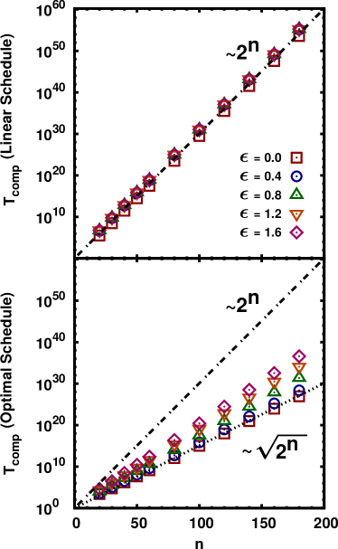
noisy Grover problem. Fig. 1 shows the scaling behavior of Tcompsubscript𝑇compT_{\text{comp}} by varying the level of noise, using either a linear schedule (Top) or an optimal schedule (Bottom) tailored to the noise model, but independent of the specific target state |σketsuperscript𝜎\Ket{\sigma^{*}} (see Appendix C and D). In both cases we employ the standard driver Hamiltonian. We observe that, for the linear schedule, neither quantum speedup nor noise effects are observed. The optimal schedule, instead, gives rise to a quadratic quantum speedup in the noiseless case that is, interestingly, only partially canceled when local disorder is taken into account. 
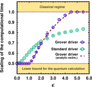
We also compared the performance of an adiabatic quantum optimizer when the standard driver Hamiltonian is substituted with the Grover-style driver Hamiltonian, in order to see how much the choice of the driver influences the “robustness” of the AQO to local noise (see Fig. 2): In this case, the Grover-style driver preserves all the quadratic quantum speedup if the noise is maintained below a certain threshold ϵϵ~less-than-or-similar-toitalic-ϵ~italic-ϵ\epsilon\lesssim\tilde{\epsilon}, but the AQO speedup quickly degrades for moderate disorder until the classical scaling is finally reached. The turning point ϵ~1~italic-ϵ1\tilde{\epsilon}\approx 1 corresponds to the noise threshold for which the lowest energy of Hdissubscript𝐻disH_{\text{dis}} is comparable with the energy of the target state (see Appendix C for more details). Conversely, the standard driver Hamiltonian appears significantly more “robust” at large disorder, so that the performance of the adiabatic QC gently decreases for increasing strength of the noise. These are good news for the possibility of implementing adiabatic QC in realistic systems since one can retain all the quantum speedup (for very weak disorder) or most of it (for moderate disorder) by choosing the appropriate driver Hamiltonian.

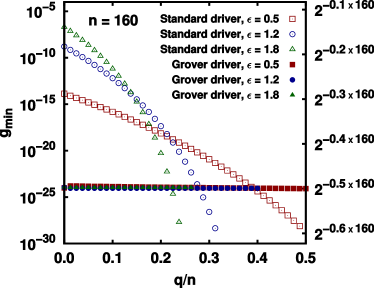
In the following, we analyze the effect of different driver Hamiltonians by observing the behavior of the minimum gap at various $q/n$ ratios for the specific system size $n=160$. As a reminder, we have denoted by $q$ the number of spins where the disorder provides a positive energy contributions. Fig. 3 shows that the minimum gap is practically independent of both $q/n$ and $\epsilon$ when the Grover driver is used: This could be expected since, for its nature, $H_{D}^{(G)}$ does not see any underlying structure of the problem energy landscape, not even the noise contribution, and presents a minimum gap only influenced by the degeneracy of the ground state (in our case, we have a unique ground state as long as $q\leq q_{\epsilon}$). On the contrary, the energy landscape plays a role during the adiabatic evolution with $H_{D}^{(S)}$ and this can be easily observed for the special case $q=0$. In this case, Eq. (C) assumes the form

$\displaystyle H^{\prime}_{\text{AQO}}$ $\displaystyle=-sn\Ket{0}\!\!\Bra{0}-\sum_{i=1}^{n}\Big{[}s|\epsilon_{i}|\hat{\sigma}_{i}^{z}+(1-s)\hat{\sigma}_{i}^{x}\Big{]},$ (33)

and the target state $\Ket{0}\!\!\Bra{0}$ is also the ground state of $-\sum_{i=1}^{n}s|\epsilon_{i}|\hat{\sigma}_{i}^{z}$. For small $\epsilon\ll 1$ one recovers the case of the noiseless Grover problem, while for large $\epsilon\gg 1$ the situation is analogous to the Hamming weight problem that presents a gap largely independent of $n$. The fact that the absolute value of the minimum gap at small $q/n$ is always larger for the standard driver (even for $\epsilon<1$ when the scaling of the computational time is better with the Grover driver) can be understood observing that the size of the minimum gap is only one of three factors that influence $T_{\text{comp}}$; the other two being the shape of the minimum gap (especially its width in the adiabatic coordinate $s$) and the probability that a certain $q/n$ is realized in practice.

Refer to caption
Figure 3: Minimum gap calculated for both the standard driver and Grover driver Hamiltonian applied to the Grover search problem with local disorder. In the first case, $g_{\text{min}}$ spans several orders of magnitude if either $q$ or ${\epsilon}$ are varied. In the latter case, the minimum gap is, instead, almost constant and scales as ${g_{\text{min}}=1/\sqrt{2^{n}}}$. This plot is obtained for systems of $n=160$ qubits. The symbols are plotted only for those $q/n$ such that $q<q_{\epsilon}$.

VI Conclusions

Estimation of the computational power of the adiabatic quantum optimization requires the knowledge of the spectral gap of the total Hamiltonian $H_{\text{AQO}}(s)$. Its direct quantification is a hard task since it requires the calculation of eigenvalues of matrices which are exponentially large in the number of qubits. To circumvent this limitation, several methods have been proposed to diminish the classical resources necessary to represent the adiabatic quantum optimizer. However, these special-purpose approaches are based on the exploitation of symmetries of either the driver or the problem Hamiltonian, and are therefore confined to particular classes of problems.

Here, we present and discuss a method that reduces the effective dimensionality of the system even in absence of explicit symmetries, and that goes beyond the idea of studying the properties and structure of the driver and problem terms separately. Formally, this is made possible by the identification of a hidden block diagonal structure in the total Hamiltonian and, consequently, by the existence of a small subspace in which the relevant eigenstates are effectively confined. According to the specific total Hamiltonian $H_{\text{AQO}}$, the present method requires only the knowledge of quantities that can be computed either analytically or by using efficient numerical approaches.

We apply the proposed method to calculate the energy gap, in a numerically exact way, for large systems exposed to local disorder or other forms of imprecision in the values of the parameter that characterize the problem Hamiltonian: Interestingly, we show that adiabatic quantum computation seems to be robust enough to deal with a form of stochastic local noise that is hardly avoidable in any real quantum device. We also find that, although the Grover driver Hamiltonian is potentially faster in the weak noise limit, the standard driver Hamiltonian, which is actually more suitable to be implemented in existing quantum hardware, results less sensitive to discrete noise.

Acknowledgments

The authors thank Peter J. Love and Sergey Knysh for many useful discussions. This work was supported by the Air Force Office of Scientific Research under Grants FA9550-12-1-0046. A.A.-G. was supported by the National Science Foundation under award CHE-1152291. A.A.-G. thanks the Corning Foundation for their generous support. The authors also acknowledge the Harvard Research Computing for the use of the Odyssey cluster.

Author contributions

S.M. and A.A.G. designed the research; S.M and G.G.G designed and devised the software for the numerical analysis, performed the research and analyzed the data; S.M, G.G.G and A.A.G. wrote the paper.

These authors contributed equally to the paper.

Appendix

Appendix A Definition of “computational time” for an adiabatic quantum optimizer

In this appendix Section we provide a precise analysis of the concept of computational time required to achieve a solution of the problem at hand. In particular, we are interested to the case in which a larger probability of success may be achieved if the adiabatic quantum optimizer is used for a shorter evolution time, but in repeated runs Boixo2014 ; Ronnow2014 . This strategy trivially includes the possibility of performing a unique, long optimization run.

Let us define $p_{S}(T)$ as the probability of success of the adiabatic quantum optimizer at fixed evolution time $T$. Recalling that the probability to (always) fail after $k$ attempts is given by $(1-p_{S}(T))^{k}$, the minimum number $K(T)$ of attempts to have a probability of $99\%$ to find the correct solution (at least once) results

$$K(T)=\frac{\log(1-0.99)}{\log(1-p_{S}(T))}\,,$$ (34)

which leads to the definition of the computational time:

$$T_{\text{comp}}=\min_{T}\Big{\{}T\cdot K(T)\Big{\}}=\min_{T}\Big{\{}T\cdot\frac{\log(1-0.99)}{\log(1-p_{S}(T))}\Big{\}}.$$ (35)

As one can deduce from its definition, it is clear that $T_{\text{comp}}\leq T^{*}$, where $T^{*}$ is the minimum evolution time to have $p_{S}(T^{*})=0.99$.

Consider now the case in which the quantum adiabatic optimizer has a hidden parameter $q$, which is different from run to run and extracted from a distribution $p(q)$. To give an explicit example, $q$ might take into account how the stochastic local noise relates to the target state for the Grover problem, as described in Section V. In this case, the probability of success of the quantum optimizer has to be averaged over the possible values of the hidden parameter and becomes

$$\bar{p}_{S}(T)=\sum_{q}p(q)\,p_{S}(q,\,T),$$ (36)

where $p_{S}(q,\,T)$ is the probability of success at fixed $q$. Consequently, the computational time takes the form

$$T_{\text{comp}}=\min_{T}\Big{\{}T\cdot\frac{\log(1-0.99)}{\log(1-\bar{p}_{S}(T))}\Big{\}}.$$ (37)

Assume that, for any given $q$, it is possible to exactly compute the spectral gap $g(s,\,q)$ at any time step $s$ of the adiabatic optimization. Therefore, an optimal schedule tailored for that specific $q$ can be constructed, as described in Roland2002 , which has an optimal evolution time given by

$$T_{\text{ann}}(q)\propto\int_{0}^{1}\frac{ds}{g^{2}(s,\,q)}\,.$$ (38)

Since the calculation of the probability of success in Eq. (36) requires the evolution of the initial quantum state throughout the whole adiabatic calculation, we adopt two main simplifications to avoid this extra overhead. First, we assume that the optimal schedule obtained for a specific $q^{*}$ is not a good adiabatic schedule for any other $q\neq q^{*}$, i.e. that the probability of any other $q\neq q^{*}$ is identically zero

$$p_{S}(q,\,T|\,q^{*})=\delta(q-q^{*})p_{S}(q^{*},\,T|\,q^{*})\,.$$ (39)

Second, we reduce the probability of success for $q^{*}$ to be a step function which is different from zero only if $T>T_{\text{ann}}(q^{*})$, namely

$$p_{S}(q^{*},\,T|\,q^{*})=\Theta(T-T_{\text{ann}}(q^{*}))\,.$$ (40)

Notice that both the above simplifications are quite conservative since we exclude the possibility that an optimal schedule works (even partially!) for any other $q$ and that the probability of success is strictly zero even for moderate evolution times. Combining Eq. (39) and Eq. (40), the computational time in Eq. (35) assumes the form

$\displaystyle T_{\text{comp}}$ $\displaystyle=\min_{T}\Big{\{}T\cdot\frac{\log(1-0.99)}{\log(1-\bar{p}_{S}(T))}\Big{\}}$
$\displaystyle=\min_{T,\,q^{*}}\Big{\{}T\cdot\frac{\log(1-0.99)}{\log(1-p(q^{*})\Theta(T-T_{\text{ann}}(q^{*})))}\Big{\}}$
$\displaystyle=\min_{q^{*}}\Big{\{}T_{\text{ann}}(q^{*})\cdot\frac{\log(1-0.99)}{\log(1-p(q^{*})))}\Big{\}}.$ (41)

It is important to notice that Eq. (A) depends only on quantities like $T_{\text{ann}}(q^{*})$ and $p(q^{*})$ which are properties of the model and not of the single run. For example, for the Grover problem with noise in Section V, both $T_{\text{ann}}(q^{*})$ and $p(q^{*})$ are completely determined by the noise model.

Appendix B “Tunneling” model: Barrier around global minimum

Here, we want to study a simple model that can be exactly solved using the exponential reduction method. The peculiarity of this model is that the ground state of the problem is surrounded by a “high-energy barrier” and, therefore, is hard to reach for a classical simulated annealer. However, AQC might find the ground state very quickly due to the tunneling effect as conjectured in Ref. reichardt2004quantum ; Farhi2002b . This example also demonstrates that our method can give rise to an exponential reduction in the dimensionality even for problems where the gap behaves sub-exponentially, i.e. when the gap closes only polynomially.

Consider the simple problem Hamiltonian corresponding to the Hamming weight problem

$$H_{P}=-\sum_{i=1}^{n}\hat{\sigma}_{i}^{z}\,,$$ (42)

which has a unique ground state, namely the configuration with all spins pointing up, and a very simple energy landscape. The main idea is to add a barrier around this unique ground state, that is to say we want to add a potential of the form

$$V(\sigma)=\begin{cases}V_{\alpha}&\text{if }w(\sigma)=1\\ 0&\text{otherwise},\end{cases}$$ (43)

with $\alpha=\{1,\,\ldots,\,n\}$ the position of the single spin which is pointing down, $V_{\alpha}>0$ (but $V_{\alpha}<0$ can be also used) and $w(\cdot)$ the Hamming weight function. Let us define $\Ket{\alpha}$ as the state in which all the spins are up apart from the $\alpha-$th spin which points down. Therefore, the problem Hamiltonian becomes

$$H_{P}=-\sum_{i=1}^{n}\hat{\sigma}_{i}^{z}+\sum_{\alpha=1}^{n}V_{\alpha}\Ket{\alpha}\!\!\Bra{\alpha}.$$ (44)

Using the standard driver Hamiltonian $H_{D}^{(S)}=-\sum_{i=1}^{n}\hat{\sigma}_{i}^{x}$, the AQO Hamiltonian results

$\displaystyle H_{\text{AQO}}$ $\displaystyle=-(1-s)\sum_{i=1}^{n}\hat{\sigma}_{i}^{x}-s\sum_{i=1}^{n}\hat{\sigma}_{i}^{z}+s\,\sum_{\alpha=1}^{n}V_{\alpha}\Ket{\alpha}\!\!\Bra{\alpha}$
$\displaystyle=-\sqrt{s^{2}+(1-s)^{2}}\,\sum_{i=1}^{n}H_{i}(s)+s\,\sum_{\alpha=1}^{n}V_{\alpha}\Ket{\alpha}\!\!\Bra{\alpha}$ (45)
$\displaystyle=-\sqrt{s^{2}+(1-s)^{2}}\,\sum_{i=1}^{n}H_{i}(s)+s\,H_{B}\,,$

where $H_{B}$ is the barrier term and all $H_{i}(s)$ are identical single spin operators which act on the $i-$th spin and whose explicit expression is given by:

$\displaystyle H_{i}(s)$ $\displaystyle=\tfrac{1-s}{\sqrt{s^{2}+(1-s)^{2}}}\hat{\sigma}_{i}^{x}+\tfrac{s}{\sqrt{s^{2}+(1-s)^{2}}}\hat{\sigma}_{i}^{z}$
$\displaystyle=\cos(\varphi_{s})\hat{\sigma}_{i}^{x}+\sin(\varphi_{s})\hat{\sigma}_{i}^{z}\,.$ (46)

Since each $H_{i}(s)$ is a rotated Pauli matrix, it has eigenvalues $\pm 1$ with corresponding eigenstates

$\displaystyle\Ket{\phi_{s}^{+}}$ $\displaystyle=\frac{1}{\sqrt{2}}\left(\sqrt{1+\sin(\varphi_{s})}\Ket{0}+\sqrt{1-\sin(\varphi_{s})}\Ket{1}\right)$
$\displaystyle=\cos(\theta_{s})\Ket{0}+\sin(\theta_{s})\Ket{1}\,$
$\displaystyle\Ket{\phi_{s}^{-}}$ $\displaystyle=\frac{1}{\sqrt{2}}\left(\sqrt{1-\sin(\varphi_{s})}\Ket{0}-\sqrt{1+\sin(\varphi_{s})}\Ket{1}\right)$
$\displaystyle=\sin(\theta_{s})\Ket{0}-\cos(\theta_{s})\Ket{1}\,,$ (47)

with $\theta_{s}=\tfrac{\varphi_{s}}{2}$. Let us call $\Ket{\phi^{+}_{i}(s)}$ and $\Ket{\phi^{-}_{i}(s)}$ the two eigenstates of $H_{i}(s)$ for any $s$. At this point, it is simple to understand that the Hamiltonian $\sum_{i=1}^{n}H_{i}(s)$ has exactly $n+1$ energy levels characterized by the number of $\Ket{\phi^{+}_{i}(s)}$ and $\Ket{\phi^{-}_{i}(s)}$ states in the product eigenstate. In the $\{\Ket{\phi^{\pm}}\}$ basis, the states in the computational basis can be written as

$$\Ket{0}=\cos(\theta_{s})\Ket{\phi_{s}^{+}}+\sin(\theta_{s})\Ket{\phi_{s}^{-}}$$ (48a)
and
$$\Ket{1}=\sin(\theta_{s})\Ket{\phi_{s}^{+}}-\cos(\theta_{s})\Ket{\phi_{s}^{-}}.$$ (48b)

It is important to observe here that all the $\theta_{s}$ depend only on $s$ and not on the spin index $i$ since all local $H_{i}(s)$ are identical. Interestingly, the Hamiltonian in Eq. (B) is the sum of two parts: an Hamiltonian for which we know exactly the eigenenergies/eigenstates for any $s$ and an Hamiltonian which non trivially acts only on $n$ states. Therefore, this model can be exponentially reduces by using our method.

Before writing the explicit form of the overlap matrix, we introduce a simplified notation in which $k(E)$ represent the number of $\Ket{\phi_{s}^{-}}$ states in each eigenvalue of energy $E$ of $\sum_{i}H_{i}(s)$. With intuitive change of notation:

$\displaystyle E(k)$ $\displaystyle=2k-n,$
$\displaystyle P_{\Omega_{E(k)}}$ $\displaystyle=P_{k},$
$\displaystyle\mathcal{Z}_{\alpha}(E(k))$ $\displaystyle=\mathcal{Z}_{\alpha}(k),$
$\displaystyle\Ket{E(k)_{\alpha}}$ $\displaystyle=\Ket{k_{\alpha}}=\frac{P_{k}\Ket{\alpha}}{\mathcal{Z}_{\alpha}(k)},$
$\displaystyle\lambda_{E(k)}$ $\displaystyle=\lambda_{k}=\binom{n}{k}.$ (49)

we can calculate

$\displaystyle\mathcal{Z}_{\alpha}(k)$ $\displaystyle=\sqrt{\Braket{\alpha}{P_{\Omega_{E}}}{\alpha}}$
$\displaystyle=\sqrt{\tbinom{n}{k}}\sqrt{\tfrac{k}{n}|\Braket{\phi_{s}^{-}}{1}|^{2}\,|\Braket{\phi_{s}^{-}}{0}|^{2(k-1)}\,|\Braket{\phi_{s}^{+}}{0}|^{2(n-k)}+\tfrac{n-k}{n}|\Braket{\phi_{s}^{+}}{1}|^{2}\,|\Braket{\phi_{s}^{-}}{0}|^{2k}\,|\Braket{\phi_{s}^{+}}{0}|^{2(n-k-1)}}$
$\displaystyle=\sqrt{\tbinom{n}{k}}|\cos(\theta_{s})|^{n-k}|\sin(\theta_{s})|^{k}\sqrt{\tfrac{k}{n}\tan^{-2}(\theta_{s})+\tfrac{n-k}{n}\tan^{2}(\theta_{s})}$ (50)
$\displaystyle\Braket{k_{\alpha}}{k^{\prime}_{\beta}}$ $\displaystyle=\delta_{kk^{\prime}}\,\frac{1}{\mathcal{Z}_{\alpha}(k)\mathcal{Z}_{\beta}(k)}\Braket{\alpha}{P_{k}}{\beta}$
$\displaystyle=\delta_{kk^{\prime}}\,\mathcal{O}_{\alpha\beta}(k)\,.$ (51)

The last line of Eq. (51) can be considered as the definition of the overlap matrix $\mathcal{O}$ given in the basis $\left\{\ket{k_{\alpha}}\right\}_{\alpha,k}$. The explicit expressions for the overlap matrix is (including the normalization):

$\displaystyle\mathcal{O}_{\alpha\alpha}(k)$ $\displaystyle=1\,,$
$\displaystyle\mathcal{O}_{\alpha\beta}(k)$ $\displaystyle=\frac{1}{n-1}\frac{-2k(n-k)+k(k-1)\tan^{-2}(\theta_{s})+(n-k)(n-k-1)\tan^{2}(\theta_{s})}{k\tan^{-2}(\theta_{s})+(n-k)\,,\tan^{2}(\theta_{s})}$ (52)

where, obviously, $\beta\neq\alpha$. Observe that the overlap element does not directly depend on $\alpha,\beta$.

Finally, adopting the same notation as in Section IV.3 we obtain the explicit form of both terms composing the reduced Hamiltonian $H_{\text{eff}}$ in the basis $\{\Ket{\mathcal{E}_{\mu}}\}$ $\Big{(}$notice that in our simplified notation we have $\Ket{\mathcal{E}^{\prime}_{\mu}}\equiv\Ket{\mathcal{E}^{(E^{\prime})}_{\mu}}$ $\Big{)}$:

$\displaystyle\Braket{\mathcal{E}_{\mu}}{H_{B}}{\mathcal{E}^{\prime}_{\nu}}$ $\displaystyle=\sum_{\alpha=1}^{n}V_{\alpha}\Braket{\mathcal{E}_{\mu}}{\alpha}\Braket{\alpha}{\mathcal{E}^{\prime}_{\nu}}=\mathcal{Z}_{\alpha}(E)\,\mathcal{Z}_{\alpha}(E^{\prime})\sum_{\alpha=1}^{n}V_{\alpha}\Braket{\mathcal{E}_{\mu}}{E_{\alpha}}\Braket{E^{\prime}_{\alpha}}{\mathcal{E}^{\prime}_{\nu}}$
$\displaystyle=\mathcal{Z}_{\alpha}(E)\,\mathcal{Z}_{\alpha}(E^{\prime})\left(\sum_{\alpha=1}^{n}V_{\alpha}\,T^{(E)}_{\mu\alpha}T^{(E^{\prime})*}_{\nu\alpha}\right)=\mathcal{Z}_{\alpha}(E)\,\mathcal{Z}_{\alpha}(E^{\prime})\left[T^{(E)}T^{(E^{\prime})\dagger}\right]_{\mu\nu}\,,$ (53a)
$\displaystyle\Braket{\mathcal{E}_{\mu}}{\Sigma_{i}H_{i}(s)}{\mathcal{E}^{\prime}_{\nu}}$ $\displaystyle=E\,\delta_{EE^{\prime}}\,\delta_{\mu\nu}\,.$ (53b)

Where $\alpha,\beta=1,\ldots,n$ are the indices corresponding to the states in $H_{B}=\sum_{\alpha=1}^{n}V_{\alpha}\Ket{\alpha}\!\!\Bra{\alpha}$, while $\mu,\nu=1,\ldots,\kappa(E)$ are the indices labeling the orthonormal basis states of the effective subspace of each $\Omega_{E}$ (i.e. neglecting the state spanning $\omega_{E}$).

Appendix C Grover Problem with local noise (Standard Driver)

In this appendix Section, we will show how to apply our method for the Grover problem in presence of local noise when the standard driver Hamiltonian is used. In the next Section, we will show briefly the derivation when a Grover-style driver Hamiltonian is used instead. Consider the following Grover problem Hamiltonian

$$H_{P}=-n\Ket{\omega}\!\!\Bra{\omega}+H_{\text{dis}},$$ (54)

where $H_{\text{dis}}=\sum_{i=1}^{n}\epsilon_{i}\hat{\sigma}_{i}^{z}$ plays the role of local disorder. If the standard driver Hamiltonian is used, the AQO Hamiltonian results

$$H_{\text{AQO}}=-sn\Ket{\omega}\!\!\Bra{\omega}+s\sum_{i=1}^{n}\epsilon_{i}\hat{\sigma}_{i}^{z}-(1-s)\sum_{i=1}^{n}\hat{\sigma}_{i}^{x}.$$ (55)

It is important to observe that the presence of the noise $\epsilon_{i}$ in Eq. (C) breaks the spin-exchange symmetry. Therefore, no methods that explicitly exploit that kind of symmetry can be used in this context. In the following, we will show that the spectral gap of the Hamiltonian in Eq. (C) can be calculated in a subspace whose dimension is exponentially reduced (compared to $2^{n}$), even in presence of local disorder. It is important to stress that our method allows the calculation of the spectral gap without any perturbative expansion around the small noise limit.

To begin with, let us apply a unitary transformation on Eq. (C) in order to get rid of the sign of all $\epsilon_{i}$, namely

$\displaystyle H^{\prime}_{\text{AQO}}$ $\displaystyle=-sn\Ket{\omega^{\prime}}\!\!\Bra{\omega^{\prime}}-s\sum_{i=1}^{n}|\epsilon_{i}|\hat{\sigma}_{i}^{z}-(1-s)\sum_{i=1}^{n}\hat{\sigma}_{i}^{x}$
$\displaystyle=-sn\Ket{\omega^{\prime}}\!\!\Bra{\omega^{\prime}}-\sum_{i=1}^{n}\Big{[}s|\epsilon_{i}|\hat{\sigma}_{i}^{z}+(1-s)\hat{\sigma}_{i}^{x}\Big{]}$
$\displaystyle=s\,H_{B}+\gamma(s)\,H_{A}.$ (56)

where $\gamma(s)=\sqrt{(s|\epsilon|)^{2}+(1-s)^{2}}$ and

$\displaystyle H_{A}$ $\displaystyle=-\sum_{i=1}^{n}\left[\frac{s|\epsilon_{i}|}{\gamma(s)}\hat{\sigma}_{i}^{z}+\frac{(1-s)}{\gamma(s)}\hat{\sigma}_{i}^{x}\right],$ (57a)
$\displaystyle H_{B}$ $\displaystyle=-n\Ket{\omega^{\prime}}\!\!\Bra{\omega^{\prime}}.$ (57b)

Since we want to maintain the number of energy levels of $H_{A}$ polynomial in the number of spins, we will consider the simple case where the noise is binomial, aka $\epsilon_{i}=|\epsilon|\delta_{i}$ with $\delta_{i}=\pm 1$. Observe that it is possible to have an exponential reduction even if the value of any $|\epsilon_{i}|$ is chosen from a finite set of $p$ distinct (possibly incommensurable) values: In this case, the number of energy levels $M$ of $H_{A}$ is upper bounded by $M\leq(n+1)^{p}$.

Refer to caption
Figure 4: Application of the proposed reduction method for the multi-solutions Grover problem. (Left panel) Difference in energy between the ground state and the $l-$th excited state, at fixed number of solutions $k=5$ and number of spins $n=60$. (Right panel) Difference in energy between the ground state and the $k-$th excited state, by varying the number of solutions $k$ at fixed number of spins $n=60$.

Therefore, the Hamiltonian $H_{B}$ in Eq. (C) becomes

$$H_{A}=-\sum_{i=1}^{n}\Big{[}\sin(\varphi_{s})\,\hat{\sigma}_{i}^{z}+\cos(\varphi_{s})\,\hat{\sigma}_{i}^{x}\Big{]}=-\sum_{i=1}^{n}\hat{\sigma}_{i}(s),$$ (58)

with $\sin(\varphi_{s})=\frac{s|\epsilon|}{\gamma(s)}$ and $\cos(\varphi_{s})=\frac{(1-s)}{\gamma(s)}$. As shown in Appendix B, all the $\hat{\sigma}_{i}(s)$ are identical and their eigenstates (corresponding to the eigenvalues $\pm 1$) are

$\displaystyle\Ket{\phi_{s}^{+}}$ $\displaystyle=\frac{1}{\sqrt{2}}\left(\sqrt{1+\sin(\varphi_{s})}\Ket{0}+\sqrt{1-\sin(\varphi_{s})}\Ket{1}\right)$
$\displaystyle=\cos(\theta_{s})\Ket{0}+\sin(\theta_{s})\Ket{1},$ (59a)
$\displaystyle\Ket{\phi_{s}^{-}}$ $\displaystyle=\frac{1}{\sqrt{2}}\left(\sqrt{1-\sin(\varphi_{s})}\Ket{0}-\sqrt{1+\sin(\varphi_{s})}\Ket{1}\right)$
$\displaystyle=\sin(\theta_{s})\Ket{0}-\cos(\theta_{s})\Ket{1}.$ (59b)

By inverting the above expressions, states in the computational basis can be expressed as

$\displaystyle\Ket{0}$ $\displaystyle=\cos(\theta_{s})\Ket{\phi_{s}^{+}}+\sin(\theta_{s})\Ket{\phi_{s}^{-}},$ (60a)
$\displaystyle\Ket{1}$ $\displaystyle=\sin(\theta_{s})\Ket{\phi_{s}^{+}}-\cos(\theta_{s})\Ket{\phi_{s}^{-}}.$ (60b)

Let us assume that $q=|\omega^{\prime}|$. Since the contribution $H_{A}$ to the Hamiltonian $H^{\prime}_{\text{AQO}}$ as expressed in Eq. (C) is invariant by spin exchange, we can always assume that all the spins in $\omega^{\prime}$ are ordered, namely $\omega^{\prime}=\Ket{0\cdots 01\cdots 1}$ (but note that the total Hamiltonian $H^{\prime}_{\text{AQO}}$ still violates the spin exchange symmetry!). Using the same notation as introduced in Appendix B, we write

$\displaystyle E(k)$ $\displaystyle=2k-n,$
$\displaystyle P_{\Omega_{E(k)}}$ $\displaystyle=P_{k},$
$\displaystyle\mathcal{Z}_{E(k)}$ $\displaystyle=\mathcal{Z}_{k},$
$\displaystyle\Ket{E(k)}$ $\displaystyle=\Ket{k}=\frac{P_{k}\Ket{\omega^{\prime}}}{\mathcal{Z}_{k}},$
$\displaystyle\lambda_{E(k)}$ $\displaystyle=\lambda_{k}=\binom{n}{k},$ (61)

where $k$ is formally the number of $\Ket{\phi_{s}^{-}}$ in a given eigenstate of $H_{B}$ at energy $E$. $\lambda_{k}$ is the degeneracy of the energy level $E$. Given the Hamiltonian in Eq. (58) and an arbitrary state in the computational base $\Ket{\omega^{\prime}}$, the normalization factor $\mathcal{Z}_{k}$ can explicitly computed:

$$\mathcal{Z}^{2}_{k}=\Braket{\omega^{\prime}}{P_{k}}{\omega^{\prime}}=\sum_{l=0}^{\min\{k,\,q\}}\!\!\!\binom{q}{l}\binom{n-q}{k-l}\sin(\theta_{s})^{2(q-l)+2(k-l)}\cos(\theta_{s})^{2n-2(q-l)-2(k-l)}.$$ (62)

Observe that if $\sin(\theta_{s})=\cos(\theta_{s})=\tfrac{1}{\sqrt{2}}$ (namely when the disorder $|\epsilon_{i}|\to 0$), the normalization factor becomes $\mathcal{Z}_{k}=2^{-n/2}\sqrt{\binom{n}{k}}$ for any choice $\omega^{\prime}$, as expected.

Appendix D Grover Problem with local noise (Grover-style Driver)

In this appendix Section, we want to derive the exponential reduction for the Grover problem in the presence of noise, when a Grover-style Hamiltonian is used instead of the standard driver Hamiltonian (see Section C). Observe that since the partitioning of the $H_{AQO}$ is different in the two cases, the final reduced Hamiltonian have completely different forms. As in Section C, let us consider the following Grover problem Hamiltonian

$$H_{P}=-n\Ket{\omega}\!\!\Bra{\omega}+H_{\text{dis}},$$ (63)

where $H_{\text{dis}}=\sum_{i=1}^{n}\epsilon_{i}\hat{\sigma}_{i}^{z}$ plays the role of local disorder. Adding the Grover-style driver Hamiltonian, the AQO Hamiltonian results

$$H_{\text{AQO}}=-sn\Ket{\omega}\!\!\Bra{\omega}+s\sum_{i=1}^{n}\epsilon_{i}\hat{\sigma}_{i}^{z}-(1-s)\Ket{\psi_{0}}\!\!\Bra{\psi_{0}},$$ (64)

where $\Ket{\psi_{0}}=\frac{1}{\sqrt{2^{n}}}\sum_{z}\Ket{z}$ is the equal superposition of all the states in the computational basis. After the application of an unitary transformation to get rid of all the sign of $\epsilon_{i}$, the AQO Hamiltonian becomes

$\displaystyle H^{\prime}_{\text{AQO}}$ $\displaystyle=-sn\Ket{\omega^{\prime}}\!\!\Bra{\omega^{\prime}}-s\sum_{i=1}^{n}|\epsilon_{i}|\hat{\sigma}_{i}^{z}-(1-s)n\Ket{\psi_{0}}\!\!\Bra{\psi_{0}}$
$\displaystyle=n\Big{(}-s\Ket{\omega^{\prime}}\!\!\Bra{\omega^{\prime}}-(1-s)\Ket{\psi_{0}}\!\!\Bra{\psi_{0}}\Big{)}-s\sum_{i=1}^{n}|\epsilon_{i}|\hat{\sigma}_{i}^{z}$
$\displaystyle=H_{B}+s\,H_{A},$ (65)

where

$\displaystyle H_{A}$ $\displaystyle=-\sum_{i=1}^{n}|\epsilon_{i}|\hat{\sigma}_{i}^{z},$ (66a)
$\displaystyle H_{B}$ $\displaystyle=-n\Big{(}s\Ket{\omega^{\prime}}\!\!\Bra{\omega^{\prime}}+(1-s)\Ket{\psi_{0}}\!\!\Bra{\psi_{0}}\Big{)}.$ (66b)

As in Section C, we choose $\epsilon_{i}=|\epsilon|\delta_{i}$ with $\delta_{i}=\pm 1$. Therefore, $H_{A}$ assumes the simple form of a rescaled Hamming weight function, namely:

$$H_{A}=-|\epsilon|\sum_{i=1}^{n}\hat{\sigma}^{z}_{i}.$$ (67)

Once defined $E(k)=2k-n$ and $P_{k}$ respectively the energy and the projector of the eigenspaces of $H_{A}$, it is straightforward to follow Section IV.3 and identify the relevant states in order to construct the reduced Hamiltonian:

$\displaystyle\Ket{E_{k}}$ $\displaystyle=\frac{P_{k}\Ket{\psi_{0}}}{\mathcal{Z}_{k}},$ (68a)
$\displaystyle\mathcal{Z}_{k}$ $\displaystyle=2^{-n/2}\sqrt{\binom{n}{k}},$ (68b)
$\displaystyle\Ket{\omega^{\prime}}$ $\displaystyle=\alpha\Ket{E_{q}}+\sqrt{1-\alpha^{2}}\Ket{\mathcal{E}},$ (68c)

where $q$ is the Hamming weight of $\omega^{\prime}$, $\alpha=1/\sqrt{\binom{n}{q}}$ and $\Ket{\mathcal{E}}$ is an appropriate eigenstate which is orthogonal to $\Ket{E_{q}}$ and lives in the $k-$th eigenspace of $H_{A}$. Notice that the presence of $\Ket{\omega^{\prime}}$ in Eq. (D) adds only one extra states (formally $\Ket{\mathcal{E}}$) because $P_{k}\Ket{\omega^{\prime}}=\delta_{kq}\Ket{\omega^{\prime}}$, where $\delta_{kq}$ is the Kronecker delta.

Appendix E Grover problem with multiple solutions

In this appendix Section, we derive the exponential reduction for the Grover problem when more solutions (i.e. target states) are acceptable. As described in Section IV.2, the AQO Hamiltonian for the multi-solution Grover problem using the standard driver Hamiltonian can be restricted to at most $k\times n$ orthogonal states, where $k$ and $n$ are, respectively, the number of solutions and the number of spins composing the database register.

Let $\{\Ket{w_{1}},\,\ldots,\,\Ket{w_{k}}\}$ being the states representing the solutions of the Grover problem. Their projections onto the eigenspaces of the standard driver Hamiltonian can be written as

$$\Ket{E_{\alpha}}=\frac{P_{\Omega_{E}}\Ket{w_{\alpha}}}{\mathcal{Z}_{\alpha}(E)}=\sqrt{1/\binom{n}{u(E)}}\sum_{x|w(x)=k}(-1)^{x\cdot w}\Ket{w},$$ (69)

where $u(E)=(E+n)/2$ represents the number of spin up at a given energy $E$ of the driver Hamiltonian, $x$ is an arbitrary bit configuration, and $w(x)$ is the Hamming weight. After some combinatorial analysis, the overlap matrix $\Braket{E_{\alpha}}{E_{\beta}}$ results to be:

$$\Braket{E_{\alpha}}{E_{\beta}}=1/\binom{n}{u(E)}\sum_{l=0}^{\min\{d_{\alpha\beta},\,u(E)\}}(-1)^{l}\binom{d_{\alpha\beta}}{l}\binom{n-d_{\alpha\beta}}{u(E)-l},$$ (70)

where $d_{\alpha\beta}$ is the Hamming distance between $\omega_{\alpha}$ and $\omega_{\beta}$. As expected, if $d=0$ the overlap is identically $1$, as well as if $u(E)=0$.

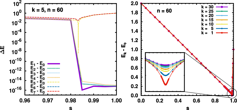
In Fig. 4, left panel, we show the difference in energy between the ground state and the $l-$th excited state, at fixed number of solutions $k=5$ and number of spins $n=60$, while in the right panel we show the difference in energy between the ground state and the $k-$th excited state, by varying the number of solutions $k$ at fixed number of spins $n=60$. As expected, the energy spectrum is $k-$degenerate at $s=1$, meaning that all the $k$ solutions belong to the reduced subspace obtained through our method to exponentially reduced the effective dimensionality.

References

  • [1] Edward Farhi, J. Goldstone, S. Gutmann, J. Lapan, A. Lundgren, and D. Preda. A quantum adiabatic evolution algorithm applied to random instances of an NP-complete problem. Science, 292(5516):472–475, April 2001.
  • [2] P. Ray, B. K. Chakrabarti, and Arunava Chakrabarti. Sherrington-Kirkpatrick model in a transverse field: Absence of replilca symmetry breaking due to quantum fluctuations. Physical Review B, 39(16):11828, 1989.
  • [3] Tadashi Kadowaki and Hidetoshi Nishimori. Quantum annealing in the transverse Ising model. Physical Review E, 58(5):5355, 1998.
  • [4] A. B. Finnila, M. A. Gomez, C. Sebenik, C. Stenson, and J. D. Doll. Quantum annealing: A new method for minimizing multidimensional functions. Chemical Physics Letters, 219(March):343–348, 1994.
  • [5] Yong-Han Lee and B. J. Berne. Global optimization: Quantum thermal annealing with path integral Monte Carlo. The Journal of Physical Chemistry A, 104(1):86–95, 2000.
  • [6] Ryan Babbush, Alejandro Perdomo-Ortiz, B. O’Gorman, William G. Macready, and Alán Aspuru-Guzik. Construction of energy functions for lattice heteropolymer models: Efficient encodings for constraint satisfaction programming and quantum annealing. Advances in Chemical Physics, 155:201, 2012.
  • [7] Rolando D Somma, Daniel Nagaj, and Mária Kieferová. Quantum speedup by quantum annealing. Physical review letters, 109(5):050501, 2012.
  • [8] Alejandro Perdomo-Ortiz, Neil Dickson, Marshall Drew-Brook, Geordie Rose, and Alán Aspuru-Guzik. Finding low-energy conformations of lattice protein models by quantum annealing. Scientific reports, 2, 2012.
  • [9] Jérémie Roland and Nicolas J. Cerf. Quantum search by local adiabatic evolution. Physical Review A, 65(4):042308, March 2002.
  • [10] Edward Farhi, Jeffrey Goldstone, and Sam Gutmann. Quantum adiabatic evolution algorithms with different paths. arXiv: quant-ph/0208135, pages 1–10, 2002.
  • [11] Saurya Das, Randy Kobes, and Gabor Kunstatter. Adiabatic quantum computation and Deutsch’s algorithm. Physical Review A, 65(6):062310, June 2002.
  • [12] Zhaohui Wei and Mingsheng Ying. A modified quantum adiabatic evolution for the Deutsch-Jozsa problem. Physics Letters A, 354(4):271–273, June 2006.
  • [13] Boris Altshuler, Hari Krovi, and Jérémie Roland. Anderson localization makes adiabatic quantum optimization fail. Proceedings of the National Academy of Sciences, 107(28):12446–12450, 2010.
  • [14] Vicky Choi. Different adiabatic quantum optimization algorithms for the NP-complete exact cover problem. Proceedings of the National Academy of Sciences USA, 108(7):E19–20, March 2011.
  • [15] Wim van Dam, Michele Mosca, and Umesh Vazirani. How powerful is adiabatic quantum computation? Proceedings of the 42nd IEEE Symposium on Foundations of Computer Science, pages 279 – 287, 2001.
  • [16] Dorit Aharonov, Wim van Dam, Julia Kempe, Zeph Landau, Seth Lloyd, and O. Regev. Adiabatic quantum computation is equivalent to standard quantum computation. SIAM Review, 50(4):755–787, 2008.
  • [17] David Deutsch and Richard Jozsa. Rapid Solution of Problems by Quantum Computation. Proc. R. Soc. Lond. A, 439(1907):553–5585, 1992.
  • [18] Lov K. Grover. A fast quantum mechanical algorithm for database search. Proceedings of the Twenty-Eighth Annual ACM Symposium on Theory of Computing STOC ’96, 1996.
  • [19] Peter W. Shor. Polynomial-time algorithms for prime factorization and discrete logarithms on a quantum computer. SIAM Review, 41(2):303–332, 1999.
  • [20] Daniel S. Abrams and Seth Lloyd. Quantum algorithm providing exponential speed increase for finding eigenvalues and eigenvectors. Physical Review Letters, 83(24):5162–5165, December 1999.
  • [21] Tad Hogg. Adiabatic quantum computing for random satisfiability problems. Physical Review A, 67(2):022314, February 2003.
  • [22] Alejandro Perdomo-Ortiz, Salvador E. Venegas-Andraca, and Alán Aspuru-Guzik. A study of heuristic guesses for adiabatic quantum computation. Quantum Information Processing, 10(1):33–52, March 2010.
  • [23] Itay Hen and AP Young. Solving the graph-isomorphism problem with a quantum annealer. Physical Review A, 86(4):042310, 2012.
  • [24] Elizabeth Crosson, Edward Farhi, Cedric Yen-yu Lin, Han-hsuan Lin, and Peter Shor. Different strategies for optimization using the quantum adiabatic algorithm. arXiv: 1401.7320, (4):1–17, 2014.
  • [25] Alán Aspuru-Guzik, Anthony D Dutoi, Peter J Love, and Martin Head-Gordon. Simulated quantum computation of molecular energies. Science, 309(5741):1704–1707, 2005.
  • [26] M-H Yung, J Casanova, A Mezzacapo, J McClean, L Lamata, A Aspuru-Guzik, and E Solano. From transistor to trapped-ion computers for quantum chemistry. Scientific reports, 4, 2014.
  • [27] Jarrod R McClean, John A Parkhill, and Alán Aspuru-Guzik. Feynman’s clock, a new variational principle, and parallel-in-time quantum dynamics. Proceedings of the National Academy of Sciences, 110(41):E3901–E3909, 2013.
  • [28] Alberto Peruzzo, Jarrod McClean, Peter Shadbolt, Man-Hong Yung, Xiao-Qi Zhou, Peter J Love, Alán Aspuru-Guzik, and Jeremy L O’Brien. A variational eigenvalue solver on a quantum processor. Nature Communications, 5(4213), 2014.
  • [29] Troels F. Rønnow, Zhihui Wang, Joshua Job, Sergio Boixo, Sergei V. Isakov, David Wecker, John M. Martinis, Daniel A. Lidar, and Matthias Troyer. Defining and detecting quantum speedup. Science, 345(6195):420–424, 2014.
  • [30] Giuseppe E Santoro, Roman Martoňák, Erio Tosatti, and Roberto Car. Theory of quantum annealing of an Ising spin glass. Science, 295(5564):2427–2430, 2002.
  • [31] DA Battaglia and L Stella. Optimization through quantum annealing: theory and some applications. Contemporary Physics, 47(4):195–208, 2006.
  • [32] A. Young, S. Knysh, and V. Smelyanskiy. Size dependence of the minimum excitation gap in the quantum adiabatic algorithm. Physical Review Letters, 101(17):170503, October 2008.
  • [33] Itay Hen. Excitation gap from optimized correlation functions in quantum Monte Carlo simulations. Physical Review E, 85(3):036705, 2012.
  • [34] Marko Znidaric and Martin Horvat. Exponential complexity of an adiabatic algorithm for an NP-complete problem. Physical Review A, 73(2):022329, February 2006.
  • [35] Itay Hen. Continuous-time quantum algorithms for unstructured problems. Journal of Physics A: Mathematical and Theoretical, 47(4):045305, January 2014.
  • [36] Edward Farhi, Jeffrey Goldstone, and Sam Gutmann. Quantum adiabatic evolution algorithms versus simulated annealing. arXiv: quant-ph/0201031, 2002.
  • [37] MHS Amin, Peter J Love, and CJS Truncik. Thermally assisted adiabatic quantum computation. Physical review letters, 100(6):060503, 2008.
  • [38] Mohammad H. S. Amin, Dmitri V. Averin, and James a. Nesteroff. Decoherence in adiabatic quantum computation. Physical Review A, 79:022107, 2009.
  • [39] Neil G. Dickson, M. W. Johnson, M. H. S. Amin, R. Harris, F. Altomare, A. J. Berkley, P. Bunyk, J. Cai, E. M. Chapple, P. Chavez, F. Cioata, T. Cirip, P. DeBuen, M. Drew-Brook, C. Enderud, S. Gildert, F. Hamze, J. P. Hilton, E. Hoskinson, Kamran Karimi, E. Ladizinsky, N. Ladizinsky, T. Lanting, T. Mahon, R. Neufeld, T. Oh, I. Perminov, C. Petroff, A. Przybysz, C. Rich, P. Spear, A. Tcaciuc, M. C. Thom, E. Tolkacheva, S. Uchaikin, J. Wang, A. B. Wilson, Z. Merali, and G. Rose. Thermally assisted quantum annealing of a 16-qubit problem. Nature Communications, 4(May):1903, May 2013.
  • [40] Kristen L. Pudenz, Tameem Albash, and Daniel A. Lidar. Error-corrected quantum annealing with hundreds of qubits. Nature Communications, 5:3243, February 2014.
  • [41] Albert Messiah. Quantum Mechanics. Wiley, 1958.
  • [42] Sabine Jansen, Mary-Beth Ruskai, and Ruedi Seiler. Bounds for the adiabatic approximation with applications to quantum computation. Journal of Mathematical Physics, 48(10):102111, 2007.
  • [43] Sergio Boixo, Troels F. Rønnow, Sergei V. Isakov, Zhihui Wang, David Wecker, Daniel A. Lidar, John M. Martinis, and Matthias Troyer. Evidence for quantum annealing with more than one hundred qubits. Nature Physics, 10(February):218, 2014.
  • [44] J. Lee. New Monte Carlo algorithm: Entropic sampling. Physical Review Letters, 71(2):211–214, 1993.
  • [45] Fugao Wang and D. Landau. Efficient, multiple-range random walk algorithm to calculate the density of states. Physical Review Letters, 86(10):2050–2053, March 2001.
  • [46] Ronald Dickman and A. G. Cunha-Netto. Complete high-precision entropic sampling. Physical Review E, 84(2):026701, August 2011.
  • [47] Lov K. Grover. Quantum mechanics helps in searching for a needle in a haystack. Physical Review Letters, 79(2):325–328, 1997.
  • [48] Edward Farhi and Sam Gutmann. Analog analogue of a digital quantum computation. Physical Review A, 57(4):2403–2406, April 1998.
  • [49] Edward Farhi, Jeffrey Goldstone, Sam Gutmann, and Daniel Nagaj. How to make the quantum adiabatic algorithm fail. International Journal of Quantum Information, 6(03):503–516, 2008.
  • [50] Lawrence M Ioannou and Michele Mosca. Limitations of some simple adiabatic quantum algorithms. International Journal of Quantum Information, 6(03):419–426, 2008.
  • [51] Zhenwei Cao and Alexander Elgart. On the efficiency of hamiltonian-based quantum computation for low-rank matrices. Journal of Mathematical Physics, 53(3):032201, 2012.
  • [52] P. W. Anderson. Local moments and localized states. Reviews of Modern Physics, 50(2):191–201, 1978.
  • [53] Neil Shenvi, Kenneth R. Brown, and K. Birgitta Whaley. Effects of noisy oracle on search algorithm complexity. Physical Review A, 68:052313, 2003.
  • [54] Jeremie Roland and Nicolas J. Cerf. Noise resistance of adiabatic quantum computation using random matrix theory. Physical Review A, 71:032330, 2005.
  • [55] Markus Tiersch and Ralf Schützhold. Non-Markovian decoherence in the adiabatic quantum search algorithm. Physical Review A, 75:062313, 2006.
  • [56] Davide Venturelli, Salvatore Mandrà, Sergey Knysh, Bryan O’Gorman, Rupak Biswas, and Vadim Smelyanskiy. Quantum optimization of fully connected spin glasses. Physical Review X, 5(3):031040, 2015.
  • [57] Andrew D King and Catherine C McGeoch. Algorithm engineering for a quantum annealing platform. arXiv preprint arXiv:1410.2628, 2014.
  • [58] Ben W Reichardt. The quantum adiabatic optimization algorithm and local minima. In Proceedings of the thirty-sixth annual ACM symposium on Theory of computing, pages 502–510. ACM, 2004.