Enhancing $\ell_{1}$-minimization estimates of polynomial chaos expansions using basis selection

Abstract

In this paper we present a basis selection method that can be used with $\ell_{1}$-minimization to adaptively determine the large coefficients of polynomial chaos expansions (PCE). The adaptive construction produces anisotropic basis sets that have more terms in important dimensions and limits the number of unimportant terms that increase mutual coherence and thus degrade the performance of $\ell_{1}$-minimization. The important features and the accuracy of basis selection are demonstrated with a number of numerical examples. Specifically, we show that for a given computational budget, basis selection produces a more accurate PCE than would be obtained if the basis is fixed a priori. We also demonstrate that basis selection can be applied with non-uniform random variables and can leverage gradient information.

1 Introduction

Quantifying uncertainty in a computational model is essential to building the confidence of stakeholders in the predictions of that model. Sources of uncertainty in model predictions can be broadly grouped into two classes, uncertainty arising from model structure and uncertainty arising from the model parameterization. The effect of these uncertainties must be traced through the model and the effect on the model output (prediction) needs to be quantified. In this paper we will present a method for quantifying parametric uncertainty that utilizes the strengths of Polynomial Chaos Expansions (PCE) and $\ell_{1}$-minimization.

When the computational cost of a simulation model is large, the most popular and effective means of quantifying parametric uncertainty is to construct an approximation of the response of the model output to variations in the model input. Once built, this surrogate can be interrogated cheaply, without further model evaluations, to obtain statistics of interest such as model output moments and distributions. Within the computational science community, the most widely adopted approximation methods used for Uncertainty Quantification (UQ) are based on generalized polynomial chaos expansions [21, 37], sparse grid interpolation [22, 24] and Gaussian process models [29].

Polynomial chaos expansions represent a response surface as a linear combination of orthonormal multivariate polynomials. The choice of the orthonormal polynomials is related to the distribution of the model input variables. Provided sufficient smoothness conditions are met, PCEs exhibit fast convergence – in some cases even exponential convergence can be obtained [1, 37]. In this paper we will focus on PCEs as they allow one to leverage the advantages of $\ell_{1}$-minimization for computing approximations from limited data.

The stochastic Galerkin [21, 37] and stochastic collocation [2, 26, 32, 36] methods are the two main approaches for approximating the PCE coefficients. The former is intrusive and so is only feasible when one has the ability to modify the code used to solve the governing equations of the model. Stochastic collocation, however, is a non-intrusive sampling based approach that allows the computational model to be treated as a black box. In this paper we focus on stochastic collocation which involves running the computational model with a set of realizations of the random parameters and constructing an approximation of corresponding model output.

Pseudo-spectral projection [13, 14], sparse grid interpolation [19, 22, 24, 28], probabilistic multi-element methods [18] are stochastic collocation methods which have been used effectively in many situations. These methods, however, all require structured samples and/or the ability to iteratively determine the collocation points.

Recently $\ell_{1}$-minimization has been shown to be an effective method for approximating PCE coefficients from small number of and possibly arbitrarily positioned collocation nodes [7, 16, 25, 31, 40]. These methods are very effective when the number of non-zero terms in the PCE approximation of the model output is small (i.e. sparse) or the magnitude of the PCE coefficients decay rapidly (i.e. compressible).

The efficacy of $\ell_{1}$-minimization when used to estimate PCE coefficients is dependent on the rate of the decay of the PCE coefficients, the characteristics of the stochastic collocation samples and the truncation of the PCE. The decay of the coefficients is a property of the model and cannot be adjusted to enhance $\ell_{1}$-recovery. However, the truncation of the PCE and the sampling of the model inputs can both be controlled.

Recently some attention has been given to designing sampling strategies to increase the accuracy of sparse PCE [30, 38, 39]. Almost no attention, however, has been given to the effect of the PCE truncation when using $\ell_{1}$-minimization. Typically, when using $\ell_{1}$-minimization, a total degree truncation is applied to PCE. However the number of terms in this basis grows factorially with the number of model parameters. This fast growth in the number of basis terms significantly affects the ability of $\ell_{1}$-minimization to accurately approximate PCE coefficients. To reduce the growth of a PCE basis in high dimensions a hyperbolic cross PCE truncation can be employed [7]. However, despite the slower growth of the hyperbolic truncation it can perform poorly when the ‘true’ PCE has large coefficients associated with interaction basis terms.

The goal of this paper is to present a basis selection algorithm that adaptively determines a set of PCE basis terms that enable accurate approximation of PCE coefficients using $\ell_{1}$-minimization. Specifically, we aim to:

• Present an iterative algorithm for selecting a polynomial chaos basis that, for a given computational budget, produces a more accurate PCE than would be obtained if the basis is fixed a priori.

• Demonstrate numerically that in high dimensions, for which high-order total-degree PCE bases are infeasible, basis selection allows the accurate identification of high-order terms that cannot be captured by a low-order total-degree basis.

• Demonstrate numerically that even for lower dimensional problems, for which high-order total-degree PCE bases are feasible, basis selection still produces more accurate results than a priori fixed basis sets.

• Show that basis selection can leverage function gradients, that for a given computational budget, will produce more accurate approximations than an approximation based solely on function values.

• Illustrate that basis selection can be applied with non-uniform random variables.

The remainder of this paper is organized as follows: Section 2 provides a brief summary of PCEs; Section 3 discuses how to use $\ell_{1}$-minimization for building a PCE and the need to move away from a priori-fixed PCE truncations in higher dimensions; Section 4 proposes a new method for iteratively defining PCE truncations; the properties and effectiveness of the proposed method are demonstrated numerically in Section 5; and conclusions are presented in Section 6.

2 Polynomial chaos expansions

Polynomial Chaos methods represent both the model inputs $\boldsymbol{\theta}=(\theta_{1},\ldots,\theta_{\tilde{d}})$ and model output $f(\boldsymbol{\theta})$ as an expansion of orthonormal polynomials of random variables ${\boldsymbol{\xi}}=(\xi_{1},\ldots,\xi_{d})$. Specifically we represent the random inputs as

$$\theta_{n}\approx\sum_{i=1}^{N_{\theta_{n}}}\beta_{i}\phi_{i}({\boldsymbol{\xi}}),\quad n=1,\ldots,\tilde{d}$$ (1)

and the model output as

$$f(\boldsymbol{\theta}({\boldsymbol{\xi}}))\approx\hat{f}({\boldsymbol{\xi}})=\sum_{i=1}^{N}\alpha_{i}\phi_{i}({\boldsymbol{\xi}}).$$ (2)

We refer to (1) and (2) as a polynomial chaos expansion (PCE). The PCE basis functions $\{\phi_{i}({\boldsymbol{\xi}})\}$ are tensor products of orthonormal polynomials which are chosen to be orthonormal with respect to the distribution $\rho({\boldsymbol{\xi}})$ of the random vector ${\boldsymbol{\xi}}$. That is

$$\left(\phi_{i}({\boldsymbol{\xi}}),\phi_{j}({\boldsymbol{\xi}})\right)=\int_{{I_{{\boldsymbol{\xi}}}}}\phi_{i}({\boldsymbol{\xi}})\phi_{j}({\boldsymbol{\xi}})\rho({\boldsymbol{\xi}})d{\boldsymbol{\xi}}=\delta_{ij}$$

where ${I_{{\boldsymbol{\xi}}}}$ is the range of the random variables.

The random variable (germ) ${\boldsymbol{\xi}}$ of the PCE is typically related to the distribution of the input variables. For example, if the one-dimensional input variable $\theta$ is uniform on $[a,b]$ then $\xi$ is also chosen to be uniform on [-1,1] and $\phi$ are chosen to be Legendre polynomials such that $\theta=\beta_{1}+\beta_{2}\xi=(b+a)/2+\xi(b-a)/2$. For simplicity and without loss of generality, we will assume that ${\boldsymbol{\xi}}$ has the same distribution as $\boldsymbol{\theta}$ and thus we can use the two variables interchangeably (up to a linear transformation which we will ignore).

The rate of convergence is dependent on the regularity of the response surface. If $f({\boldsymbol{\xi}})$ is analytical with respect to the random variables then (2) converges exponentially in $L_{2}(\rho({\boldsymbol{\xi}}))$-sense [6].

In practice the PCE (2) must be truncated. The most common approach is to set a degree $p$ and retain only the multivariate polynomials of degree at most $p$. Rewriting (2) using the typical multi-dimensional index notation

$$f({\boldsymbol{\xi}})\approx\hat{f}({\boldsymbol{\xi}})=\sum_{\boldsymbol{\lambda}\in\Lambda}\alpha_{\boldsymbol{\lambda}}\phi_{\boldsymbol{\lambda}}({\boldsymbol{\xi}})$$ (3)

the total degree basis of degree $p$ is given by

$$\Lambda=\Lambda^{d}_{p,q}=\{\phi_{\boldsymbol{\lambda}}:\left\lVert\boldsymbol{\lambda}\right\rVert_{q}\leq p\},\quad\boldsymbol{\lambda}=(\lambda_{1},\ldots,\lambda_{d})$$ (4)

with $q=1$. The number of terms in this total degree basis

$$\text{card}\;\Lambda^{d}_{p,1}\equiv P={d+p\choose d}$$

grows factorially with dimension. This rapid growth limits the applicability of the total degree basis to moderate dimensions or low degree polynomials in higher dimensions.

The authors of [7] propose using hyperbolic index sets, (4) with $q<1$, to slow the growth of the PCE basis with dimensionality. The use of hyperbolic indices assumes that the contribution to variance from the interaction between the random variables decays rapidly as the number of variables involved in the interaction increases. Figure 1 shows a three dimensional total degree and hyperbolic index set. It is clear that for a given degree $p$ the hyperbolic index set has many less terms than the total degree polynomial basis. However the smaller basis size requires omitting polynomial terms interaction terms, that is indices $\boldsymbol{\lambda}$ with at least two $\lambda_{n}>0,n=1,\ldots,d$. When a function has large non-zero PCE coefficients corresponding to these missing multivariate basis terms, the hyperbolic index set may be an inappropriate form of truncation. Ideally the basis truncation should be adapted to the function being approximated.

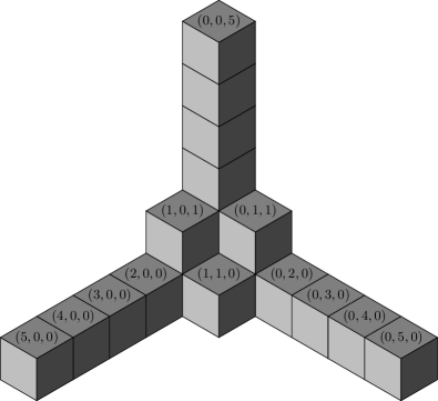
Figure 1: (Left) A total degree index set $\Lambda^{3}_{6,1}$. (Right) A hyperbolic index set $\Lambda^{3}_{6,1/2}$. Each cube represents a $3$-dimensional index $\boldsymbol{\lambda}=(\lambda_{1},\lambda_{2},\lambda_{3})$ in $\Lambda$. The value of each $\boldsymbol{\lambda}$ is given on the top of each cube.

3 $\ell_{1}$-minimization

The coefficients of a polynomial chaos expansion can be approximated effectively using $\ell_{1}$-minimization. Specifically, given a small set of $M$ unstructured realizations $\boldsymbol{\Xi}=\{{\boldsymbol{\xi}}_{1},\ldots,{\boldsymbol{\xi}}_{M}\}$, with corresponding model outputs $\mathbf{f}=(f({\boldsymbol{\xi}}_{1}),\ldots,f({\boldsymbol{\xi}}_{M}))^{T}$, we would like to find a solution that satisfies

$$\boldsymbol{\Phi}\boldsymbol{\alpha}\approx\mathbf{f}$$

where $\boldsymbol{\alpha}=(\alpha_{\boldsymbol{\lambda}_{1}},\ldots,\alpha_{\boldsymbol{\lambda}_{N}})^{T}$ denotes the vector of PCE coefficients and $\boldsymbol{\Phi}$ denotes the Vandermonde matrix with entries $\boldsymbol{\Phi}_{ij}=\phi_{j}({\boldsymbol{\xi}}_{i}),\quad i=1,\ldots,M,\;j=1,\ldots,N$.

When the model $f({\boldsymbol{\xi}})$ is high-dimensional and computationally expensive, and non-adaptive basis truncation rules are employed, the number of model simulations that can be generated is much smaller than the number of unknown PCE coefficients, i.e $M\ll N$. Under these conditions, finding the PCE coefficients is ill-posed and we must impose some form of regularization to obtain a unique solution.

$\ell_{1}$-minimization provides a means of identifying sparse coefficient vectors from a limited amount of simulation data. A polynomial chaos expansion is defined as $s$-sparse when $\left\lVert\boldsymbol{\alpha}\right\rVert_{0}\leq s$, i.e. the number of non-zero coefficients does not exceed $s$. In practice, not many simulation models will be truly sparse, but PCE are often compressible, that is the magnitude of the coefficients decay rapidly or alternatively most of the PCE variance is concentrated in a few terms. Compressible vectors are well represented by sparse vectors and thus the coefficients of compressible PCE can also be recovered accurately using $\ell_{1}$-minimization.

$\ell_{1}$-minimization attempts to find the dominant PCE coefficients by solving the following optimization problem

$$\boldsymbol{\alpha}=\operatorname*{arg\,min}_{\boldsymbol{\alpha}}\;\|\boldsymbol{\alpha}\|_{1}\quad\text{such that}\quad\|\boldsymbol{\Phi}\boldsymbol{\alpha}-\mathbf{f}\|_{2}\leq\varepsilon$$ (5)

This $\ell_{1}$-minimization problem is often referred to as Basis Pursuit Denoising. The problem obtained by setting $\varepsilon=0$, to enforce interpolation, is termed Basis Pursuit. There is a close connection between (5) and Least Absolute Shrinkage Operator (LASSO) [33] well known in the statistics literature. Indeed these problems are equivalent under certain conditions [15].

3.1 $\ell_{1}$-minimization algorithms

Numerous algorithms [5, 10, 27, 34] exist for solving (5) which are all stable and accurate under certain well defined conditions. In this paper we will use the greedy algorithm Orthogonal Matching Pursuit (OMP) [11] to estimate PCE coefficients. OMP requires stronger theoretical conditions than some of its counterparts [9] but in practice OMP can still obtain comparable accuracy to these algorithms. In this paper we use OMP because of its fast execution speed which makes OMP more amenable to cross validation which can be used to estimate optimal method parameters such as the tolerance $\varepsilon$ of (5). We remark, however, that the basis selection procedure presented in this paper can be used in conjunction with most $\ell_{1}$-minimization algorithms.

3.1.1 Hyper-parameter estimation via cross validation

Accurately computing the coefficients of a polynomial chaos expansion requires determining a ‘good’ truncation set $\Lambda$ and specifying the tolerance $\varepsilon$ in the Basis Pursuit DeNoising problem (5). Cross validation has been shown to be effective at aiding these choices. Specifically cross validation has been used in the past to estimate the polynomial degree $p$ of a hyperbolic expansion [7] and to estimate the tolerance $\varepsilon$ of (5) [7, 8, 16, 25, 35].

In this paper we will use $K=10$ fold cross validation to choose the values of sets of hyper-parameters $\boldsymbol{\gamma}$. The number and type of hyper-parameters is dependent on the $\ell_{1}$-minimization method used in conjunction with cross validation. As an example consider solving in (5) using an a priori fixed total degree basis $\Lambda_{p,1}^{d}$. The hyper-parameters that can be estimated using cross validation are the degree $p$ and the tolerance $\varepsilon$, that is $\boldsymbol{\gamma}=(p,\varepsilon)$.

Let $\zeta:\{1,\ldots,M\}\rightarrow\{1,\ldots,K\}$ be an indexing function that determines the partition of the training data. Furthermore let $\hat{f}^{-\zeta}$ be the PCE approximation built on the data with the $\zeta$ part removed, then the cross validation error is given by

$$e_{\mathrm{cv}}(\boldsymbol{\gamma})=\frac{1}{M}\sum_{k=1}^{K}e_{\zeta(k)},\quad e_{\zeta(k)}=\sum_{j\in\zeta(k)}(y_{j}-\hat{f}^{-\zeta(k)}(x_{j}))^{2}$$ (6)

To compute $e_{\mathrm{cv}}$ we divide the data pairs $(\Xi,\mathbf{f})$, based upon the randomly chosen partitions $\zeta(k)$, into $K$ sets (folds) of equal size $(\Xi_{k},\mathbf{f}_{k})$, $k=1,\ldots,K$. A PCE $\hat{f}^{-\zeta(k)}$, is then built on the training data $\Xi_{\mathrm{t}}=\Xi\setminus\Xi_{k}$ with the $k$-th fold removed, using the hyper-parameters $\boldsymbol{\gamma}$. The remaining data $\Xi_{\mathrm{v}}=\Xi_{k}$ is then used to estimate the prediction error. To estimate the hyper-parameters $\boldsymbol{\gamma}$ we search over a set of possible values for $\boldsymbol{\gamma}$ and select $\boldsymbol{\gamma}=\operatorname*{arg\,min}_{\boldsymbol{\gamma}}e_{\mathrm{cv}}(\boldsymbol{\gamma})$.

Figure 2 presents a typical example illustrating the change in the $\ell_{2}$ error of a PCE with fixed degree, as the tolerance $\varepsilon$ is decreased. The figure also plots the cross validation error which is a good indicator of the $\ell_{2}$ error behavior. The vertical line represents the tolerance chosen by cross validation and the horizontal line is the $\varepsilon_{\ell_{2}}$ error in the resulting PCE. The result shown is typical. There is a bias (underestimation of $\varepsilon_{\ell_{2}}$) in the cross validation estimate, yet despite this bias cross validation consistently chooses a tolerance that produces a near minimal error.

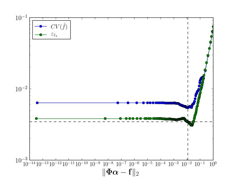
Figure 2: The use of cross validation to select the truncation tolerance $\varepsilon$ for (11) with coefficients $c^{(1)}$. The vertical line represents the tolerance chosen by cross validation and the horizontal line is the $\varepsilon_{\ell_{2}}$ error in the resulting PCE. $M=200$ uniform samples were used. Accuracy is measured using the $\ell_{2}$ norm computed at $100,000$ Latin-hypercube samples (see Section 5).

3.2 Recoverability of $\ell_{1}$-minimization

The ability of $\ell_{1}$-minimization to accurately determine the large coefficients of the PCE is determined by the properties of the matrix $\boldsymbol{\Phi}$ and the sparsity of PCE representation of the model response $f({\boldsymbol{\xi}})$. The sparsity is a property of the model and cannot be changed, however the properties of the $\boldsymbol{\Phi}$ are influenced by the selection of the realizations $\{{\boldsymbol{\xi}}_{i}\}_{i=1}^{M}$ and the truncation $\Lambda$.

Mutual coherence is one measure often used to indicate the ability of $\ell_{1}$-minimization to find a sparse solution. The mutual coherence of a matrix $\boldsymbol{\Phi}\in\mathbb{R}^{M\times N}$ with columns $\tilde{\phi}_{j}$ is

$$\mu(\boldsymbol{\Phi})=\max_{1<j<k\leq N}\frac{\left\lvert\tilde{\phi}_{j}^{T}\tilde{\phi}_{k}\right\rvert}{\left\lVert\tilde{\phi}_{j}\right\rVert_{2}\left\lVert\tilde{\phi}_{k}\right\rVert_{2}}$$ (7)

and is a measure of the maximum correlation between any two columns in the matrix. $\ell_{1}$-minimization will obtain a better estimate of the PCE coefficients if the mutual coherence of $\boldsymbol{\Phi}$ is small. Intuitively, if two columns are closely correlated the mutual coherence will be large and it will be impossible, in general, to distinguish whether the energy in the signal comes from one or the other.

The restricted isometry property (RIP) [10], quantified by the restricted isometry constant $\delta$ is another measure of the recoverability of the matrix $\boldsymbol{\Phi}$. For each $s=1,2,\ldots$ the isometry constant $\delta_{s}$ of a matrix $\boldsymbol{\Phi}$ is the smallest number such that

$$(1-\delta_{s})\left\lVert\boldsymbol{\alpha}_{s}\right\rVert_{2}^{2}\leq\left\lVert\boldsymbol{\Phi}\boldsymbol{\alpha}_{s}\right\rVert_{2}^{2}\leq(1+\delta_{s})\left\lVert\boldsymbol{\alpha}_{s}\right\rVert_{2}^{2}$$ (8)

for all vectors $\boldsymbol{\alpha}_{s}$ with $s$ non-zero entries. This is equivalent to requiring that the eigenvalues of all Grammian matrices $\boldsymbol{\Phi}^{\top}_{\Lambda_{s}}\boldsymbol{\Phi}_{\Lambda_{s}}$ lie between $[1-\delta_{s},1+\delta_{s}]$, where $\boldsymbol{\Phi}_{\Lambda_{s}}$ are $M\times s$ submatrices of $\boldsymbol{\Phi}$. The restricted isometry property measures the ability of $\boldsymbol{\Phi}$ to preserve the lengths of $s$-sparse vectors. The RIP can be intuitively thought of as a measure of $s$-wise coherence as opposed to mutual coherence which is a measure of pair wise coherence.

3.2.1 Sampling strategies and pre-conditioning

The sampling strategy used to choose the samples $\Xi$ affects the mutual coherence and RIP of $\boldsymbol{\Phi}$ and thus can impact the accuracy of the recovered polynomial chaos expansion. To date, the best sampling strategies for $\ell_{1}$-minimization are random [30, 38]. The nature of the random samples is dependent on the distribution of the random variables ${\boldsymbol{\xi}}$, the number of random dimensions, and the degree of the PCE.

The accuracy of $\ell_{1}$-minimization solutions of (5) can also be improved by the use of pre-conditioning. The pre-conditioned $\ell_{1}$-minimization problem is given by

$$\boldsymbol{\alpha}=\operatorname*{arg\,min}_{\boldsymbol{\alpha}}\;\|\boldsymbol{\alpha}\|_{1}\quad\text{such that}\quad\|\mathbf{W}\boldsymbol{\Phi}\boldsymbol{\alpha}-\mathbf{W}\mathbf{f}\|_{2}\leq\varepsilon$$ (9)

where $W\in\mathbb{R}^{M\times M}$ is a diagonal matrix with entries chosen to enhance the recovery properties of $\ell_{1}$-minimization. When recovering $s$-sparse one-dimensional Legendre polynomials, randomly sampling $\Xi=\{\xi_{m}\}_{m=1}^{M}$ from the Chebyshev measure and choosing weights $w_{m,m}=(\pi/2)^{d/2}(1-\xi_{m}^{2})^{1/4}$, can result in significant increases in the accuracy of the coefficients recovered by $\ell_{1}$-minimization [30]. In the multivariate setting, however, the benefit of pre-conditioning is less clear [39]. In this paper all numerical results presented are generated without pre-conditioning.

3.2.2 PCE truncation

Naively choosing a large degree $p$ can cause a degradation in the accuracy of the PCE coefficients. Figure 3 demonstrates that both the mutual coherence and the 10-sparse RIP constant $\delta_{10}$ of the Vandermonde matrix $\boldsymbol{\Phi}$ increases as the number of basis terms $P$ increases.

(a)

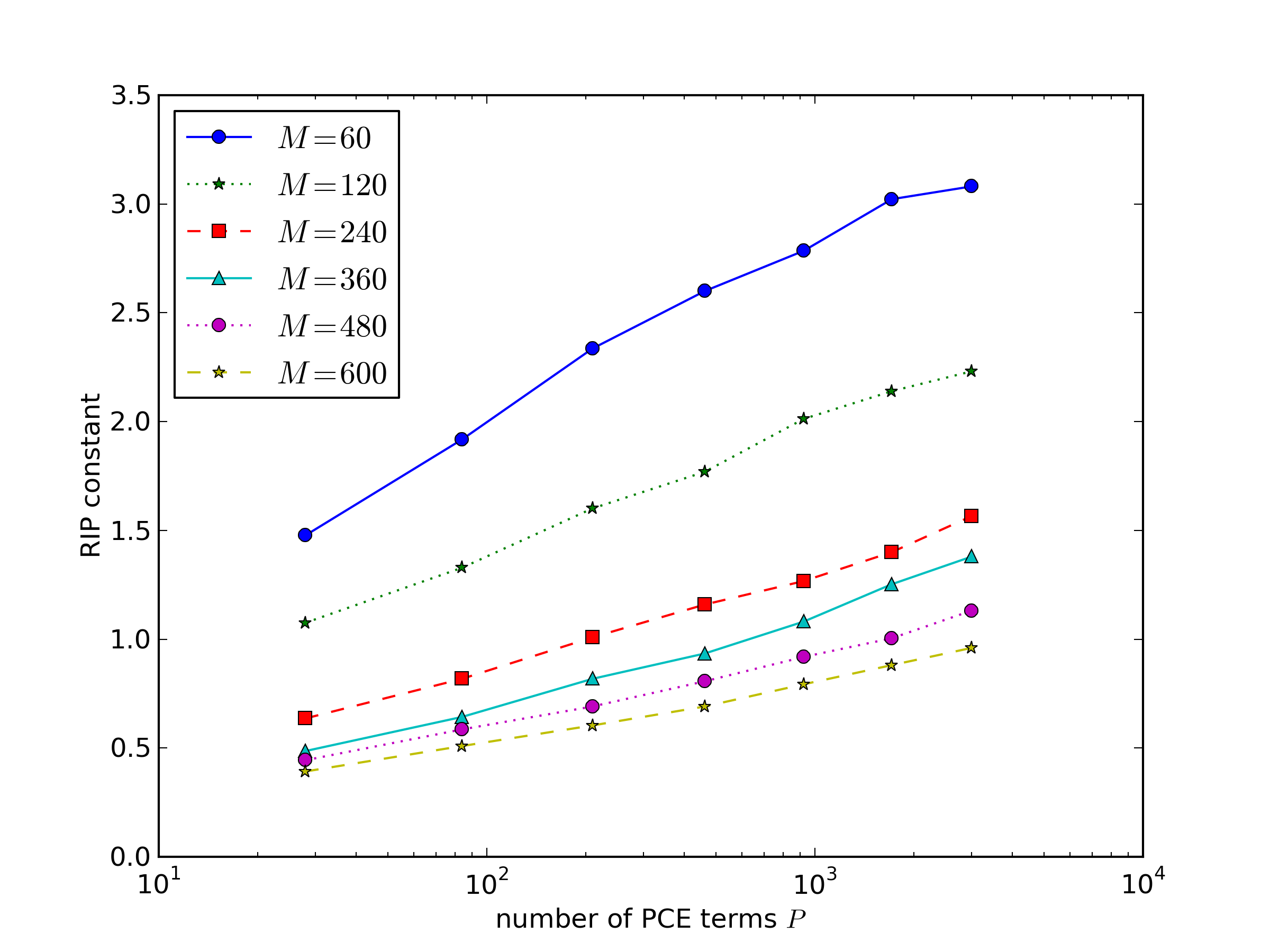
(b)

Figure 3: Growth of mutual coherence and RIP constant $\delta_{10}$ with the number of terms $P$ in a 6-dimensional total-degree multivariate Legendre PCE basis.

Increases in mutual coherence and RIP constant are correlated with a decrease in the accuracy of PCE coefficients recovered by $\ell_{1}$-minimization. Figure 4 demonstrates that, for a fixed number of samples, as the number of terms $N$ and, consequently, the mutual coherence and RIP constant increase (see Figure 3), the PCE recovered by $\ell_{1}$-minimization becomes less accurate. Figure 4 also illustrates that the accuracy of the PCE depends upon the degree of the basis used. As the number of samples $M$ increases, $\ell_{1}$-minimization is able to recover more dominant coefficients and a higher degree should be used. However for a given number of samples increasing the degree does not always lead to a reduction in error. For example when $M=60$ the PCE of total degree $p=4$ has the smallest error and at $M=120$ setting $p=7$ produces the smallest error. It is not until $M=240$ that the highest degree basis $p=8$ produces the smallest error. These results are consistent with the theoretical results in [16] that assert that the number of samples $M$ needed to recover a Legendre PCE of a certain sparsity $s$ increases with the number of terms in the PCE basis.

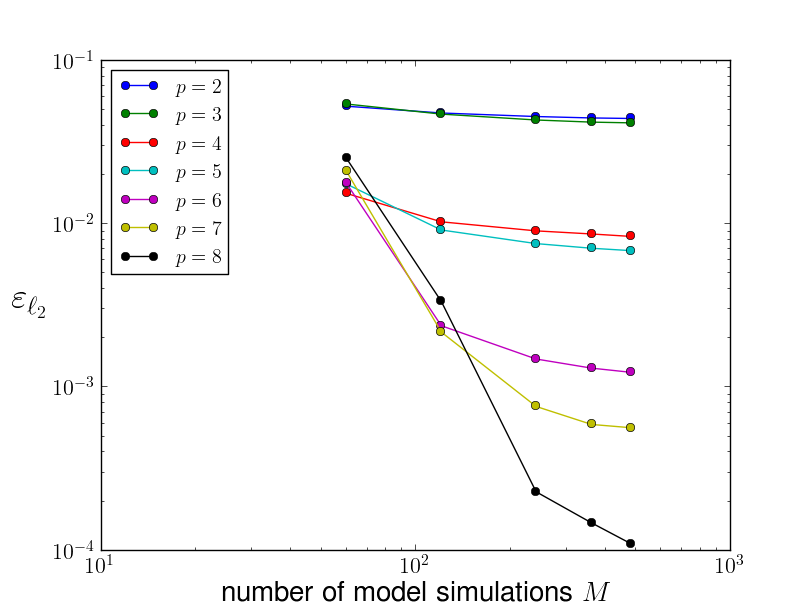
Figure 4: The dependence of PCE accuracy on the polynomial degree $p$. The $degree$ of the most accurate expansion is dependent on the number of LHS samples $M$ used to construct the PCE. Results were obtained using orthogonal matching pursuit with cross validation to choose $\varepsilon$ applied to the 6-dimensional random oscillator (12). Accuracy is measured using the $\ell_{2}$ norm computed at $100,000$ Latin-hypercube samples (see Section 5).

4 Iterative basis selection

When the coefficients of a PCE can be well approximated by a sparse vector, $\ell_{1}$-minimization is extremely effective at recovering the coefficients of that PCE. It is possible, however, to further increase the efficacy of $\ell_{1}$-minimization by leveraging realistic models of structural dependencies between the values and locations of the PCE coefficients. For example [3, 17, 23] have successfully increased the performance of $\ell_{1}$-minimization when recovering wavelet coefficients that exhibit a tree-like structure. In this vein, we propose an algorithm for identifying the large coefficients of PC expansions that form a semi-connected subtree of the PCE coefficient tree.

The coefficients of polynomial chaos expansions often form a multi-dimensional tree. Given an ancestor basis term $\phi_{\boldsymbol{\lambda}}$ of degree $\left\lVert\boldsymbol{\lambda}\right\rVert_{1}$ we define the indices of its children as $\boldsymbol{\lambda}+\mathbf{e}_{k}$, $k=1,\ldots,d$, where $\mathbf{e}_{k}=(0,\ldots,1,\ldots,0)$ is the unit vector co-directional with the $k$-th dimension. An example of a typical PCE tree is depicted in Figure 5. In this figure, as often in practice, the magnitude of the ancestors of a PCE coefficient is a reasonable indicator of the size of the child coefficient. In practice, some branches (connections) between levels of the tree may be missing. We refer to trees with missing branches as semi-connected trees.

In the following we present a method for estimating PCE coefficients that leverages the tree structure of PCE coefficients to increase the accuracy of coefficient estimates obtained by $\ell_{1}$-minimization.

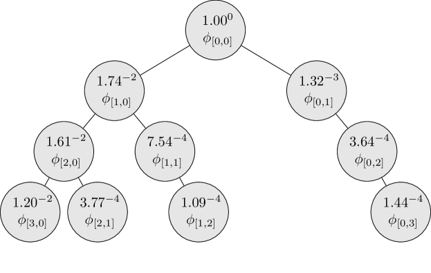
Figure 5: Tree structure of the coefficients of a two dimensional PCE with $\Lambda_{3,1}^{2}$. For clarity we only depict one connection per node, but in $d$ dimensions a node of a given degree $p$ will be a child of up to $d$ nodes of degree $p-1$. For example, not only is the basis $\boldsymbol{\phi}_{[1,1]}$ a child of $\boldsymbol{\phi}_{[1,0]}$ (as depicted) but it is also a child of $\boldsymbol{\phi}_{[0,1]}$

4.1 Algorithm

Typically $\ell_{1}$-minimization is applied to an a priori chosen and fixed basis set $\Lambda$. However the accuracy of coefficients obtained by $\ell_{1}$-minimization can be increased by adaptively selecting the PCE basis.

To select a basis for $\ell_{1}$-minimization we employ a four step iterative procedure involving restriction, expansion, identification and selection. The iterative basis selection procedure is outlined in Algorithm 1. A graphical version of the algorithm is also presented in Figure 6. The latter emphasizes the four stages of basis selection, that is restriction, growth, identification and selection. These four stages are also highlighted in Algorithm 1 using the corresponding colors in Figure 6.

To initiate the basis selection algorithm, we first define a basis set $\Lambda^{(0)}$ and use $\ell_{1}$-minimization to identify the largest coefficients $\boldsymbol{\alpha}^{(0)}$. The choice of $\Lambda^{(0)}$ can sometimes affect the performance of the basis selection algorithm. We found a good choice to be $\Lambda^{(0)}=\Lambda_{p,1}$, where $p$ is the degree that gives $\lvert\Lambda^{d}_{p,1}\rvert$ closest to $10M$, i.e. $\Lambda^{d}_{p,1}=\operatorname*{arg\,min}_{\Lambda^{d}_{p,1}\in\{\Lambda^{d}_{1,1},\Lambda^{d}_{2,1},\ldots\}}\left\lvert\lvert\Lambda^{d}_{p,1}\rvert-10M\right\rvert$. Given a basis $\Lambda^{(k)}$ and corresponding coefficients $\boldsymbol{\alpha}^{(k)}$ we reduce the basis to a set $\Lambda^{(k)}_{\varepsilon}$ containing only the terms with non-zero coefficients. This restricted basis is then expanded $T$ times using an algorithm which we will describe in Section 4.1.1. $\ell_{1}$-minimization is then applied to each of the expanded basis sets $\Lambda^{(k,t)}$ for $t=1,\dots,T$. Each time $\ell_{1}$-minimization is used, we employ cross validation to choose $\varepsilon$. Therefore, at every basis set considered during the evolution of the algorithm we have a measure of the expected accuracy of the PCE coefficients. At each step in the algorithm we choose the basis set that results in the lowest cross validation error.

$\Lambda^{\star}=\Lambda^{(0)}=\Lambda^{d}_{p,1}=\operatorname*{arg\,min}_{\Lambda^{d}_{p,1}\in\{\Lambda^{d}_{1,1},\Lambda^{d}_{2,1},\ldots\}}\left\lvert\lvert\Lambda^{d}_{p,1}\rvert-10M\right\rvert$

$\boldsymbol{\alpha}^{(0)}$, $e_{\mathrm{cv}}^{(0)}$ = $\ell_{1}$-minimization[$\boldsymbol{\Phi}(\Lambda^{(0)})$,$\mathbf{f}$]

$T=3$, $e_{\mathrm{cv}}^{\star}=\infty$, $k=1$

while TRUE do

       $e_{\mathrm{cv}}^{(k)}=\infty$

         $\Lambda^{(k,0)}=\{\boldsymbol{\lambda}:\boldsymbol{\lambda}\in\Lambda^{(k-1)},\boldsymbol{\alpha}_{\boldsymbol{\lambda}}^{(k)}\neq 0\}$

       for $t\in\{1,\ldots,T\}$ do

               $\Lambda^{(k,t)}$ = EXPAND[$\Lambda^{(k,t-1)}$]

               $\boldsymbol{\alpha}^{(k,t)}$, $e_{\mathrm{cv}}^{(k,t)}$ = $\ell_{1}$-minimization[$\boldsymbol{\Phi}(\Lambda^{(k,t)})$,$\mathbf{f}$]

             if $e_{\mathrm{cv}}^{(k,t)}<e_{\mathrm{cv}}^{(k)}$ then

                    $e_{\mathrm{cv}}^{(k)}=e_{\mathrm{cv}}^{(k,t)}$, $\boldsymbol{\alpha}^{(k)}=\boldsymbol{\alpha}^{(k,t)}$, $\Lambda^{(k)}=\Lambda^{(k,t)}$

             end if

            

       end for

      if $e_{\mathrm{cv}}^{(k)}>e_{\mathrm{cv}}^{\star}$ then

             TERMINATE

       end if

      $\alpha^{\star}=\boldsymbol{\alpha}^{(k)},\;\Lambda^{\star}=\Lambda^{(k)},\;e_{\mathrm{cv}}^{\star}=e_{\mathrm{cv}}^{(k)}$

end while

Algorithm 1 $\Lambda^{\star}$,$\boldsymbol{\alpha}^{\star}$=BASIS_SELECTION[$\boldsymbol{\Phi}$,$\mathbf{f}$,$\varepsilon$]

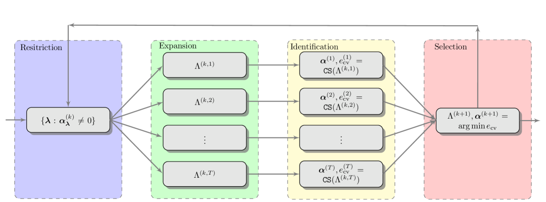
Figure 6: Graphical depiction of the basis adaptation algorithm.

4.1.1 Basis expansion

Define $\{\boldsymbol{\lambda}+\mathbf{e}_{j}:1\leq j\leq d\}$ the forward neighborhood of an index $\boldsymbol{\lambda}$ and similarly let $\{\boldsymbol{\lambda}-\mathbf{e}_{j}:1\leq j\leq d\}$ denote the backward neighborhood. To expand a basis set $\Lambda$ we must first find the forward neighbors $\mathcal{F}=\{\boldsymbol{\lambda}+\mathbf{e}_{j}:\boldsymbol{\lambda}\in\Lambda,1\leq j\leq d\}$ of all indices $\boldsymbol{\lambda}\in\Lambda$. The expanded basis is then given by

$$\Lambda^{+}=\Lambda\cup\mathcal{A},\quad\mathcal{A}=\{\boldsymbol{\lambda}:\boldsymbol{\lambda}\in\mathcal{F},\boldsymbol{\lambda}-\mathbf{e}_{n}\in\Lambda\text{ for }1\leq n\leq d,\,\lambda_{k}>1\}$$

where we have used the following admissibility criteria

$$\boldsymbol{\lambda}-\mathbf{e}_{n}\in\Lambda\text{ for }1\leq n\leq d,\,\lambda_{k}>1$$ (10)

to target PCE basis indices that are likely to have large PCE coefficients. A forward neighbor is admissible only if its backward neighbors exist in all dimensions. If the backward neighbors do not exist then $\ell_{1}$-minimization has previously identified that the coefficients of these backward neighbors are negligible.

The admissibility criterion is explained graphically in Figure 7. In the left graphic, both children of the current index are admissible, because its backwards neighbors exist in every dimension. In the right graphic only the child in the vertical dimension is admissible, as not all parents of the horizontal child exist.

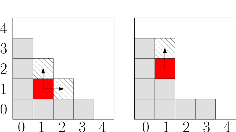
Figure 7: Identification of the admissible indices of an index (red). The indices of the current basis $\Lambda$ are gray and admissible indices are striped. A index is admissible only if its backwards neighbors exists in every dimension.

At the $k$-th iteration of Algorithm 1, $\ell_{1}$-minimization is applied to $\Lambda^{(k-1)}$ and used to identify the significant coefficients of the PCE and their corresponding basis terms $\Lambda^{(k,0)}$. The set of non-zero coefficients $\Lambda^{(k,0)}$ identified by $\ell_{1}$-minimization is then expanded. The EXPAND routine expands an index set by one polynomial degree, but sometimes it may be necessary to expand the basis $\Lambda^{(k)}$ more than once. To generate these higher degree index sets EXPAND is applied recursively to $\Lambda^{(k,0)}$ up to a fixed number of $T$ times. Specifically, the following sets are generated

$$\Lambda^{(k,t)}=\Lambda^{(k,t-1)}\cup\{\boldsymbol{\lambda}:\boldsymbol{\lambda}-\mathbf{e}_{n}\in\Lambda^{(k,t-1)},1\leq n\leq d,\,\lambda_{n}>1\}.$$

As the number of expansion steps $T$ increases the number of terms in the expanded basis increases rapidly and degradation in the performance of $\ell_{1}$-minimization can result (this is similar to what happens when increasing the degree of a total degree basis). To avoid degradation of the solution, we use cross validation to choose the number of inner expansion steps $t\in[1,T]$.

5 Numerical examples

In this section we use several numerical tests to demonstrate the benefit of the basis selection method. In each example we seek a PCE approximation to a model output given a set of uncertain parameters with a known range or distribution.

We compare the approximations constructed using basis selection against those constructed using a non-adaptive strategy. The non-adaptive strategy consists of generating basis sets $\Lambda_{2,1}^{d},\ldots,\Lambda_{p,1}^{d}$ where $p$ is the degree that produces the basis set with a cardinality closest to $100000$. $\ell_{1}$-minimization is then applied to this basis with a cross validation tolerance search to compute the non-zero polynomial coefficients. The resulting basis with the lowest cross validation error is chosen to be the final approximation.

We also compare the non-adaptive and basis selection methods against OMP using a basis oracle. For a set of $M$ model runs, the oracle method sets $\Lambda$ in (5) to be the basis of the best $M$-term PCE approximation of the function. The best $M$-term approximation is obtained by using a dimension adaptive sparse grid to calculate the ‘exact’ PCE coefficients and selecting the basis terms with the $M$ largest coefficients. This basis will be close to optimal and therefore will serve as a good estimate of the maximum accuracy that can be gained from the use of basis selection.

In order to construct a PCE approximation, the sample design has to be specified. By a design we mean the choice of sample size, $M$, and the selection $\boldsymbol{\Xi}=\{{\boldsymbol{\xi}}_{i}\}_{i=1}^{M}$ Here we opt for uniform random samples of size $M$. For small sample sizes $M$ the selection of $\boldsymbol{\Xi}$ significantly affects the performance of any approximation method. Therefore, for each $M$, twenty different designs are used to build a PCE and the mean, maximum and minimum of the resulting errors are reported. We did investigate the utility of using samples drawn from the Chebyshev measure but found that there was no consistent benefit. Even in the cases for which a benefit was observed, the improvement was small relative to the benefit gained from using basis adaptation. This finding is consistent with [39].

To measure the performance of an approximation, we will use the $\ell_{2}$ error (RMSE). Specifically given a set of $Q=100,000$ Latin-hypercube samples $\boldsymbol{\Xi}_{\text{test}}=\{{\boldsymbol{\xi}}^{(i)}\}_{i=1}^{Q}\in{I_{{\boldsymbol{\xi}}}}$ and samples of the true function $f({\boldsymbol{\xi}}^{(i)})$ and the PCE approximation $\hat{f}({\boldsymbol{\xi}}^{(i)})$ we compute

$$\varepsilon_{\ell_{2}}=\left(\frac{1}{Q}\sum_{i=1}^{Q}\lvert\hat{f}({\boldsymbol{\xi}}^{(i)})-f({\boldsymbol{\xi}}^{(i)})\rvert^{2}\right)^{1/2}$$

Note in all examples presented using Legendre polynomials we transform each $d$ dimensional parameter domain ${I_{{\boldsymbol{\xi}}}}$, build points $\boldsymbol{\Xi}$ and test points $\boldsymbol{\Xi}_{\mathrm{test}}$ to $[-1,1]^{d}$.

5.1 Algebraic test function

Consider the algebraic corner-peak test function [20]

$$f_{\mathrm{CP}}(\mathbf{x})=\left(1+\sum_{k=1}^{d}c_{k}\,\xi_{k}\right)^{-(d+1)},\quad{\boldsymbol{\xi}}\in[0,1]^{d}$$ (11)

This function provides a flexible test that can be used to identify the strengths of the proposed algorithm. Specifically, the coefficients $c_{k}$ can be used to control the effective dimensionality and the compressibility of these functions. Here we will examine performance using three different choices of $\mathbf{c}=(c_{1},\ldots,c_{d})^{T}$, specifically

$$c^{(1)}_{k}=\frac{k-\frac{1}{2}}{d},\quad c_{k}^{(2)}=\frac{1}{k^{2}}\quad\text{and}\quad c_{k}^{(3)}=\exp\left(\frac{k\log(10^{-8})}{d}\right),\quad k=1,\ldots,d$$

normalizing such that $\sum_{k=1}^{d}c_{k}=0.25$. The coefficients $\mathbf{c}^{(1)}$, $\mathbf{c}^{(2)}$ and $\mathbf{c}^{(3)}$ represent increasing levels of anisotropy and decreasing effective dimensionality. Anisotropy refers to the dependence of the function variability, often measured through variance, on individual parameter dimensions $\xi_{n}$. When a function is strongly anisotropic, the majority of the function variance can be attributed to a small set of dimensions. The size of this subset is referred to as the effective dimension.

The performance of the basis selection method is dependent on the properties of the model being approximated. Figure 8 plots the $\varepsilon_{\ell_{2}}$ error in the polynomial approximations for increasing number of model evaluations. For all three levels of anisotropy the adaptive method produces an expansion no worse than the non-adaptive method, for the same sample size. When anisotropy is introduced the accuracy of basis selection increases relative to the non-adaptive method. The stronger the anisotropy the better the relative performance. Figure 8 also plots the PCE obtained using OMP with an oracle basis. When very weak anisotropy is present $\mathbf{c}^{(1)}$, there is little that can be gained by using a well chosen basis, as evident by the lack of separation between the three convergence curves. However as the strength of the anisotropy is increased the effect of the oracle basis on accuracy becomes much more apparent. When strong anisotropy, $\mathbf{c}^{(3)}$, is present, basis selection is able to obtain the same accuracy as the oracle without a priori information on the truncation of the basis which is required by the oracle. In the moderately anisotropic $\mathbf{c}^{(2)}$ case basis selection does not perform as well as the oracle but does still perform better than the non-adaptive method.

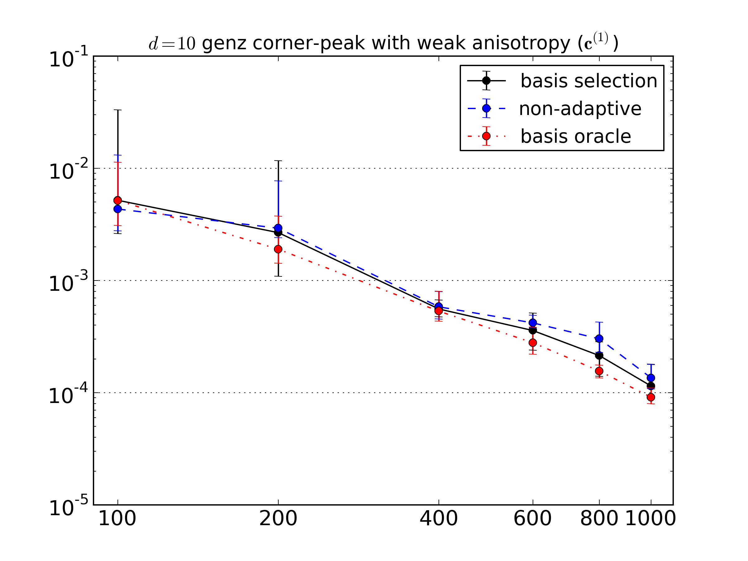
(a)

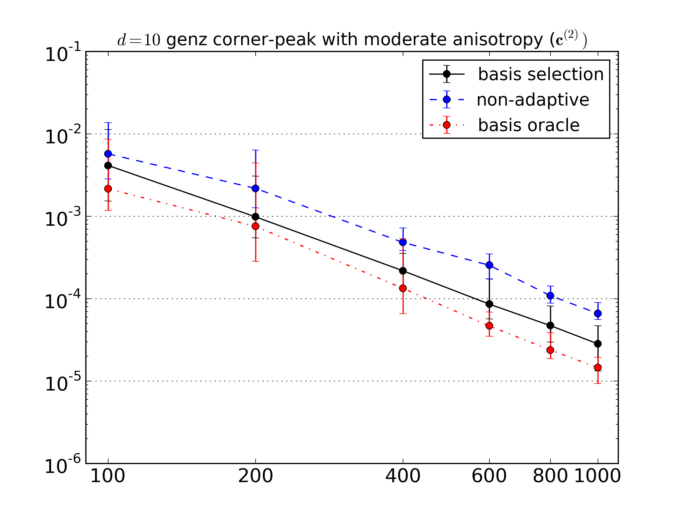
(b)

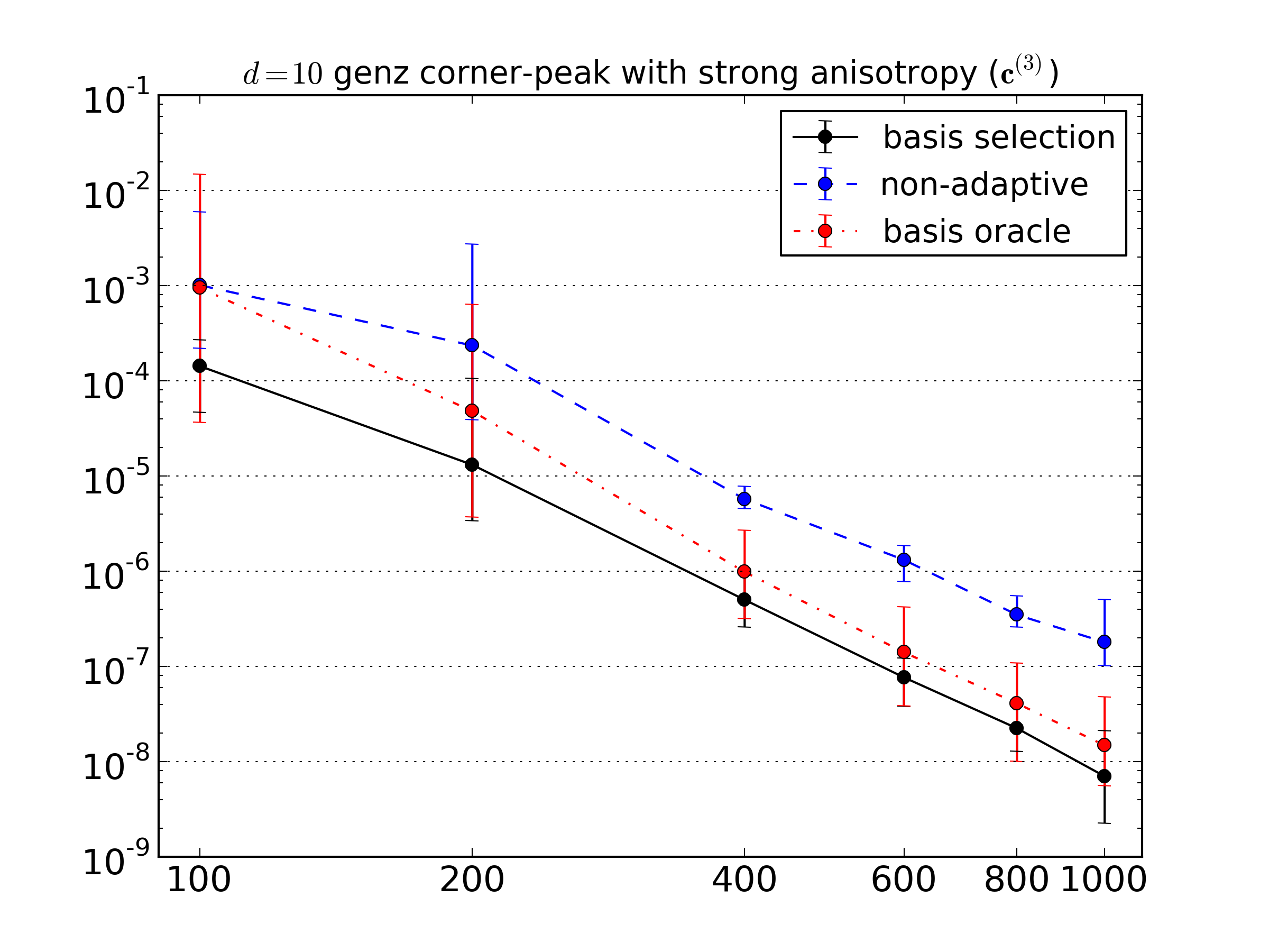
(c)

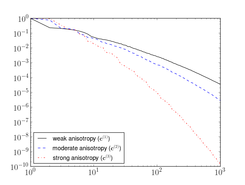
(d)

Figure 8: Convergence of the RMSE, with respect to increasing design size $M$, in the Legendre PCE approximation of the Genz corner-peak function (11) for the three coefficient regimes: (a) $\mathbf{c}^{(1)}$, (b) $\mathbf{c}^{(2)}$, (c) $\mathbf{c}^{(3)}$. The error bars represent the minimum and maximum error over the $20$ trials for each design size $M$. (d) PCE coefficients, sorted by magnitude, for the three coefficient regimes.

To understand the correlation between anisotropy and the performance of the basis selection method we must consider the the structure of the PCE coefficients induced by varying $\mathbf{c}$. Figure 8 (d) plots the decay of the PCE coefficients when sorted by magnitude. As anisotropy increases, so does the rate of decay of the sorted PCE coefficients.

It is the strength of decay that controls the performance of basis selection. When the rate of decay is high then the function is more compressible and thus better suited to being approximated using $\ell_{1}$-minimization. Anisotropy will often result in compressible coefficients, but it is conceptually possible for models to be compressible without being anisotropic. For some problems such as the elliptic Poisson equation the decay of the PCE coefficients can be calculated a-priori [1, 4, 12] but unfortunately in practice, the decay of the PCE coefficients of a model cannot be determined ahead of time. A practical means of identifying the coefficient decay regime would be very useful but is beyond the scope of this paper.

Not only does the rate of coefficient decay affect performance, but so to does the ability of the PCE basis $\Lambda$ to represent the target function. For example if the ‘true’ PCE has large high degree terms with large coefficients but the basis $\Lambda$ does not have these high degree terms then the PCE obtained using $\Lambda$ will not be as accurate as a PCE obtained using a basis that included the important high degree terms.

Figure 9 plots the exact PCE coefficients of the algebraic test function using $\mathbf{c}^{(1)}$ and $\mathbf{c}^{(3)}$. The ‘exact’ coefficients obtained using a dimension-adaptive sparse grid with $100,000$ which results in an approximation error below $10^{-8}$. In Figure 9 (a), the random variables contribute similarly to the total variance of $f_{\text{CP}}$ and so the dominant coefficients are concentrated in the lower degree terms of the PCE, thus a total degree basis set will perform as well as any alternative. In comparison, the importance of the dimensions of the function shown in Figure 9 (b) decay exponentially with dimension, which results in higher-degree terms with large coefficients in some dimensions. In this coefficient regime, if $\ell_{1}$-minimization can only be applied with a low degree polynomial (which is true when using a total degree basis), the accuracy of the resulting PCE, for a given number of samples $M$, will not be as high as a PCE constructed using a basis that includes the dominant high-degree terms. Basis selection will typically allow identification and recovery of more high-degree coefficients than would be possible if using a total degree basis.

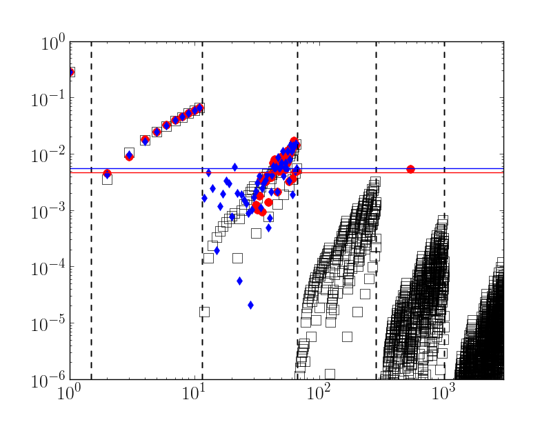
(a)

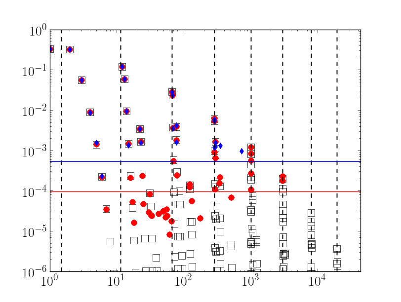
(b)

Figure 9: Comparison of PCE coefficients of $\mathbf{c}^{(1)}$ (a) and $\mathbf{c}^{(3)}$ (b). The black squares represent the ‘exact’ coefficients, the red circles the non-zero coefficients of the basis selection method and the blue diamonds are the non-zero coefficients recovered by the non-adaptive approach. The indices on the x axis are sorted lexicographically by degree. The dashed vertical lines separate the PCE terms into degrees. The horizontal lines represent the $\ell_{2}$ error in the basis selection and non-adapted PCE. The identification of more terms accurately with basis selection results in a smaller error.

5.2 Random oscillator

In this section we investigate the performance of basis selection to quantify uncertainty in a damped linear oscillator subject to external forcing with six unknown parameters. That is,

$$\frac{d^{2}x}{dt^{2}}(t,{\boldsymbol{\xi}})+\gamma\frac{dx}{dt}+kx=f\cos(\omega t),$$ (12)

subject to the initial conditions

$$x(0)=x_{0},\quad\dot{x}(0)=x_{1},$$ (13)

where we assume the damping coefficient $\gamma$, spring constant $k$, forcing amplitude $f$ and frequency $\omega$, and the initial conditions $x_{0}$ and $x_{1}$ are all uncertain. We solve (12) analytically to avoid consideration of discretization errors in our study.

Defining ${\boldsymbol{\xi}}=(\gamma,k,f,\omega,x_{0},x_{1})$ let $\xi_{1}\in[0.08,0.12]$, $\xi_{2}\in[0.03,0.04]$, $\xi_{3}\in[0.08,0.12]$, $\xi_{4}\in[0.8,1.2]$, $\xi_{5}\in[0.45,0.55]$, $\xi_{6}\in[-0.05,0.05]$. For any parameter realization in $I_{\boldsymbol{\xi}}$ the harmonic oscillator will be underdamped. In the following, we choose our quantity of interest to be the position $x(t)$ of the oscillator at $t=20$ seconds.

Figure 10 (a) depicts the error in the Legendre PCE for increasing design sizes $M$. The basis selection method clearly outperforms the non-adaptive approach and produces comparable results to the oracle. Again the improvement in performance is associated with a rapid decay of the exact PCE coefficients (see Figure 10).

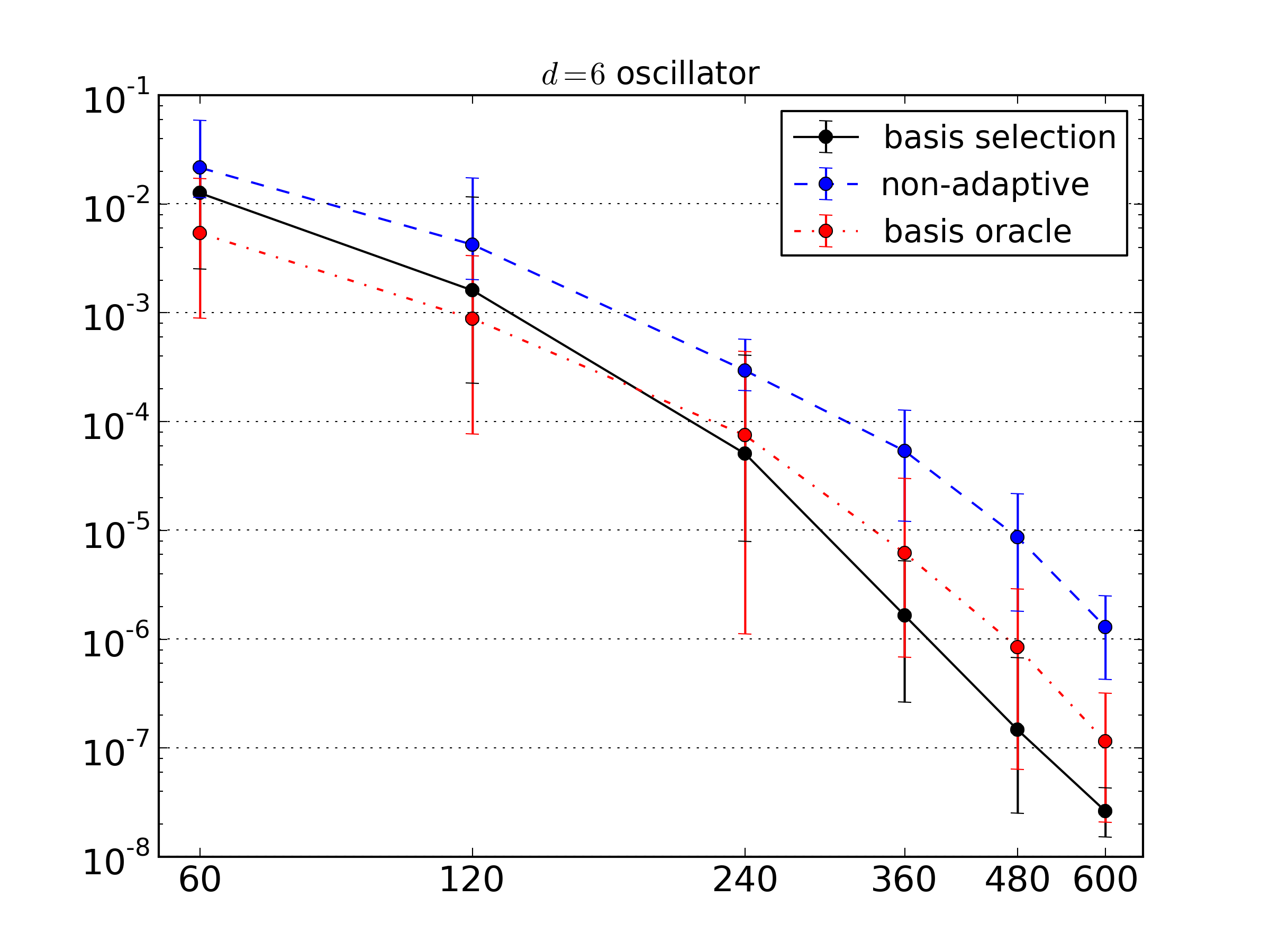
(a)

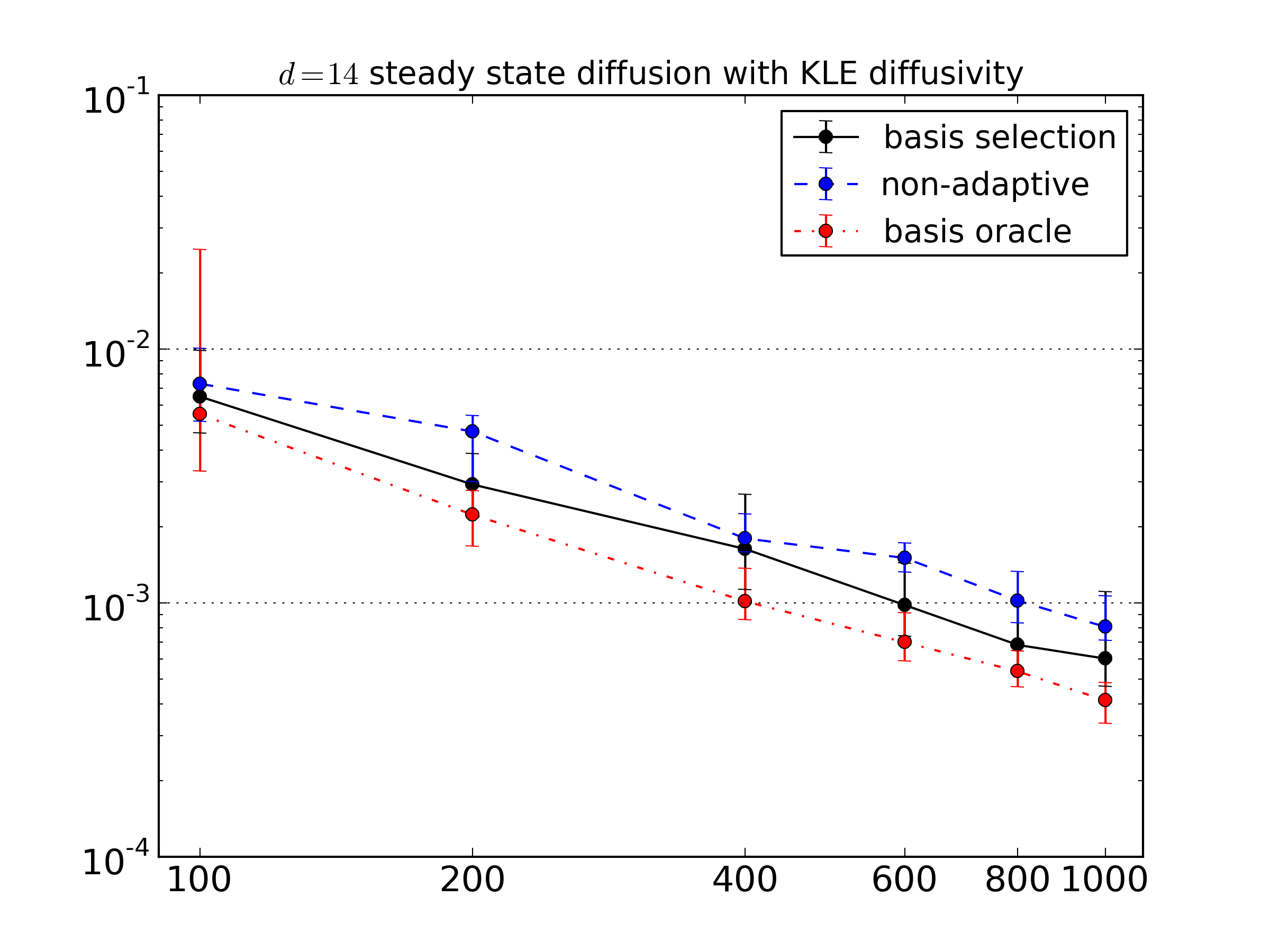
(b)

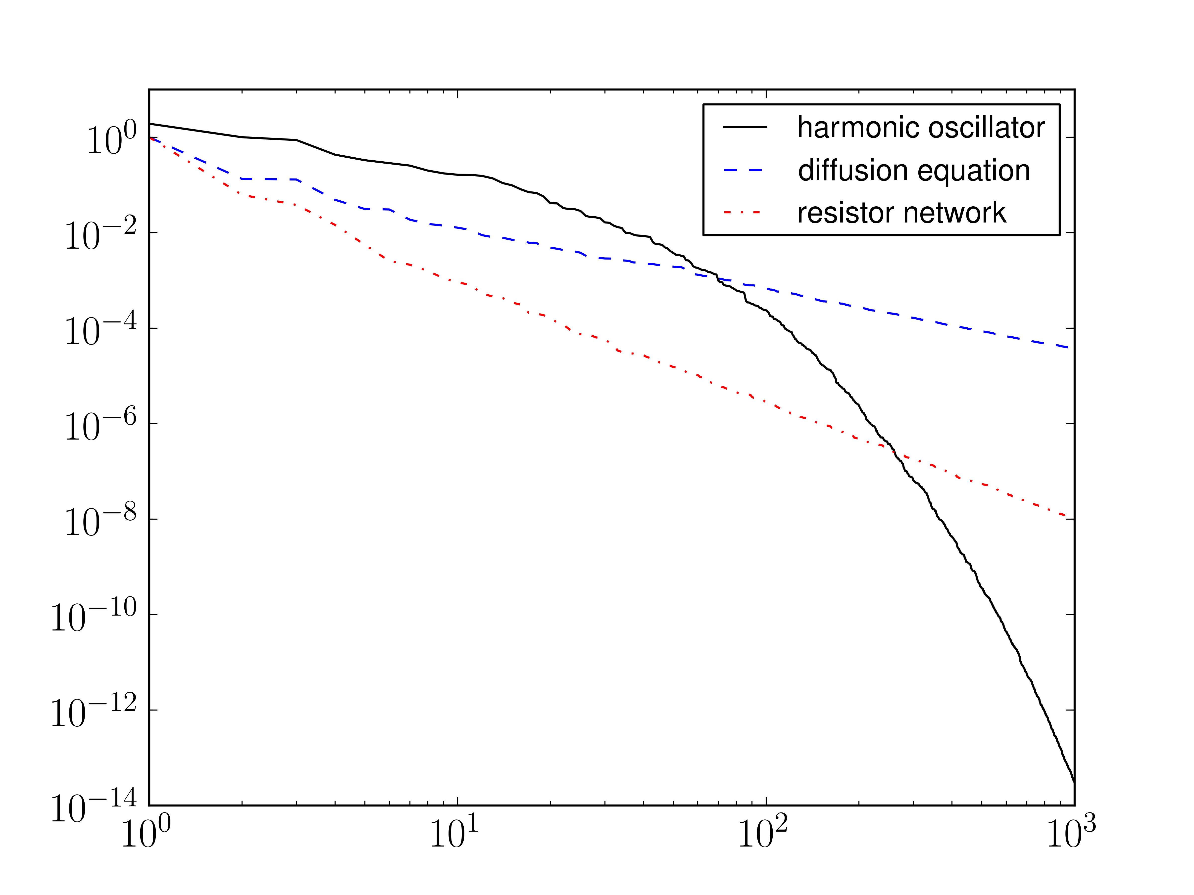
(c)

Figure 10: Convergence of the RMSE, with respect to increasing design size $M$, in the Legendre PCE approximation of (a) the harmonic oscillator (12) and (b) the solution $u(1/3,{\boldsymbol{\xi}})$ of the diffusion equation (14). The error bars represent the minimum and maximum error over the $20$ trials for each design size $M$. (c) PCE coefficients, sorted by magnitude, for the harmonic oscillator, the diffusion equation and the resistor network.

5.3 Diffusion equation

In this section, we consider the heterogeneous diffusion equation in one-spatial dimension subject to uncertainty in the diffusivity coefficient. This problem has been used as a benchmark in other works [16, 40]. Attention is restricted to one-dimensional physical space to avoid unnecessary complexity. The procedure described here can easily be extended to higher physical dimensions. Consider the following problem with $d\geq 1$ random dimensions:

$$-\frac{d}{dx}\left[a(x,{\boldsymbol{\xi}})\frac{du}{dx}(x,{\boldsymbol{\xi}})\right]=1,\quad(x,{\boldsymbol{\xi}})\in(0,1)\times I_{\boldsymbol{\xi}}$$ (14)

subject to the physical boundary conditions

$$u(0,{\boldsymbol{\xi}})=0,\quad u(1,{\boldsymbol{\xi}})=0.$$ (15)

Furthermore, assume that the random diffusivity satisfies

$$a(x,{\boldsymbol{\xi}})=\bar{a}+\sigma_{a}\sum_{k=1}^{d}\sqrt{\lambda_{k}}\phi_{k}(x)\xi_{k},$$ (16)

where $\{\lambda_{k}\}_{k=1}^{d}$ and $\{\phi_{k}(x)\}_{k=1}^{d}$ are, respectively, the eigenvalues and eigenfunctions of the squared exponential covariance kernel

$$C_{a}(x_{1},x_{2})=\exp\left[-\frac{(x_{1}-x_{2})^{2}}{l_{c}^{2}}\right].$$

The variability of the diffusivity field (16) is controlled by $\sigma_{a}$ and the correlation length $l_{c}$ which determines the decay of the eigenvalues $\lambda_{k}$. Here we approximate the solution $u(1/3,{\boldsymbol{\xi}})$ with $\bar{a}=0.1$, $d=14$, $\sigma_{a}=0.03$, $l_{c}=1/5$, while the uncertain inputs $\xi_{k}\in[-1,1]$, $k=1,\ldots,d$ are independent and uniformly distributed random variables. We solve the model (14) using quadratic finite elements with a high enough spatial resolution to neglect discretization errors in our analysis.

Figure 10 (b) plots the error in Legendre PCE approximations built using increasing design sizes $M$. There is negligible difference between basis selection and the non-adaptive strategy, but there is also negligible difference between these methods and the oracle, indicating there is not much improvement that can in principle be gained from basis selection. The negligible improvement is due to the fact that the ‘exact’ PCE is not very compressible, as can be seen from Figure 10. The lack of compressibility means that many coefficients are of similar magnitude and thus $\ell_{1}$-minimization in any form is not very effective.

5.4 Resistor network

Figure 11: Resistor network comprised of $d=2P$ resistances $R_{i}$, $i=1,\ldots,d$ of uncertain ohmage and the network is driven by a voltage source providing a known potential $V_{0}$. We are interested in determining voltage at $V$.

As our last example, consider the electrical resistor network shown in Figure 11. The network is comprised of $d=2P$ resistances of uncertain ohmage and the network is driven by a voltage source providing a known potential $V_{0}$. We are interested in determining how the voltage $V$ shown in the figure depends on the $d=2P$ resistances, which we take as random parameters uniformly distributed in the interval $\xi_{k}\in[1-\varepsilon,1+\varepsilon]$, $k=1,\ldots,d$. This function is anisotropic. The effect of the resistors on the voltage will decay with distance (in terms of the number of preceding resistors) from the point $V$. In this example we set $d=40$ ($P=20$) and $d=80$ ($P=40$), take the maximum perturbation to be $\varepsilon=0.1$ and set the reference potential $V_{0}=1$.

Figure 12 shows the error in the Legendre PCE for increasing design sizes $M$. In both cases the basis selection method produces a PCE that is significantly more accurate than the PCE produced by the non-adaptive strategy. The basis selection method provides comparable results to the approximately optimal oracle.

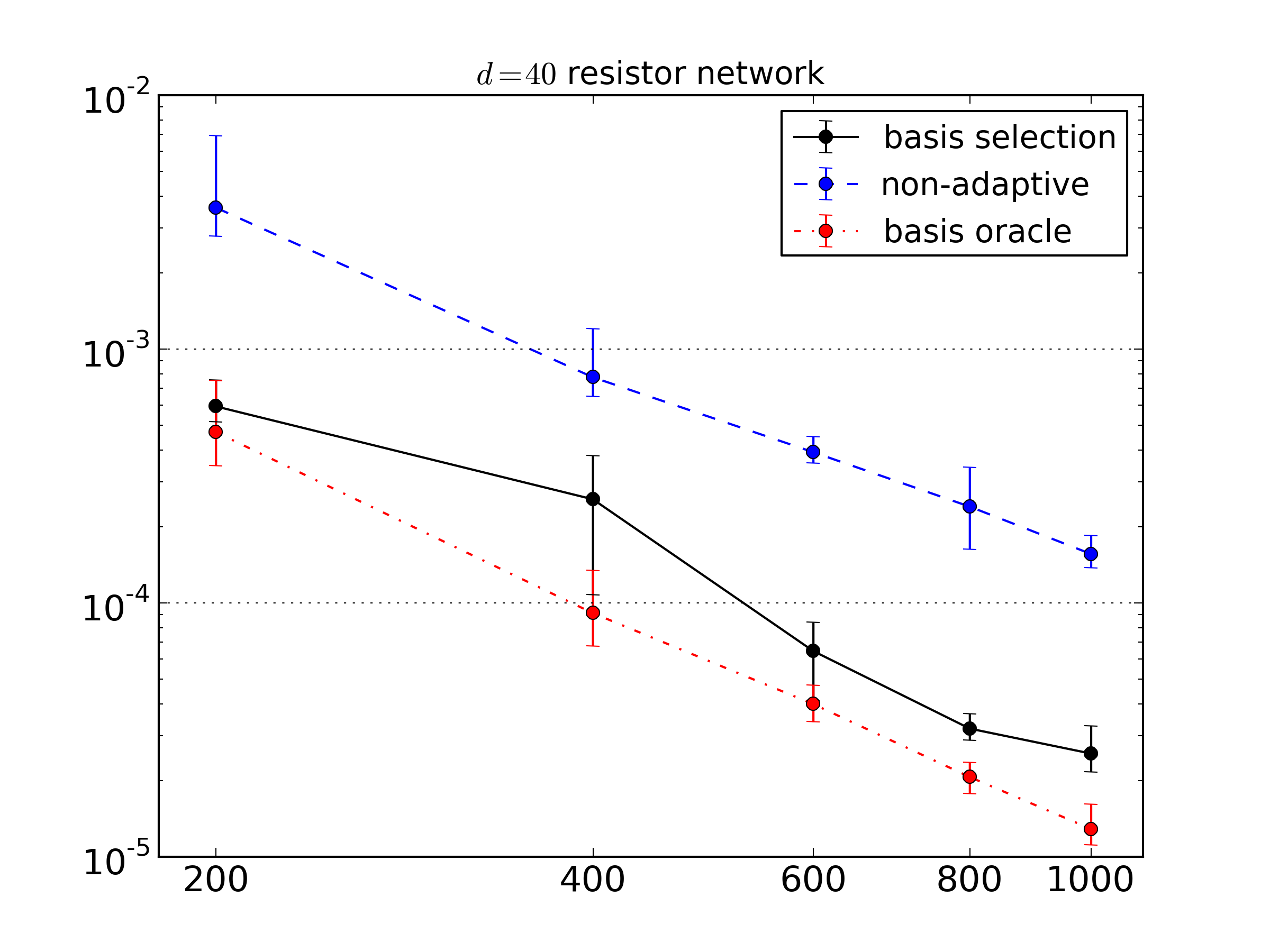
(a)

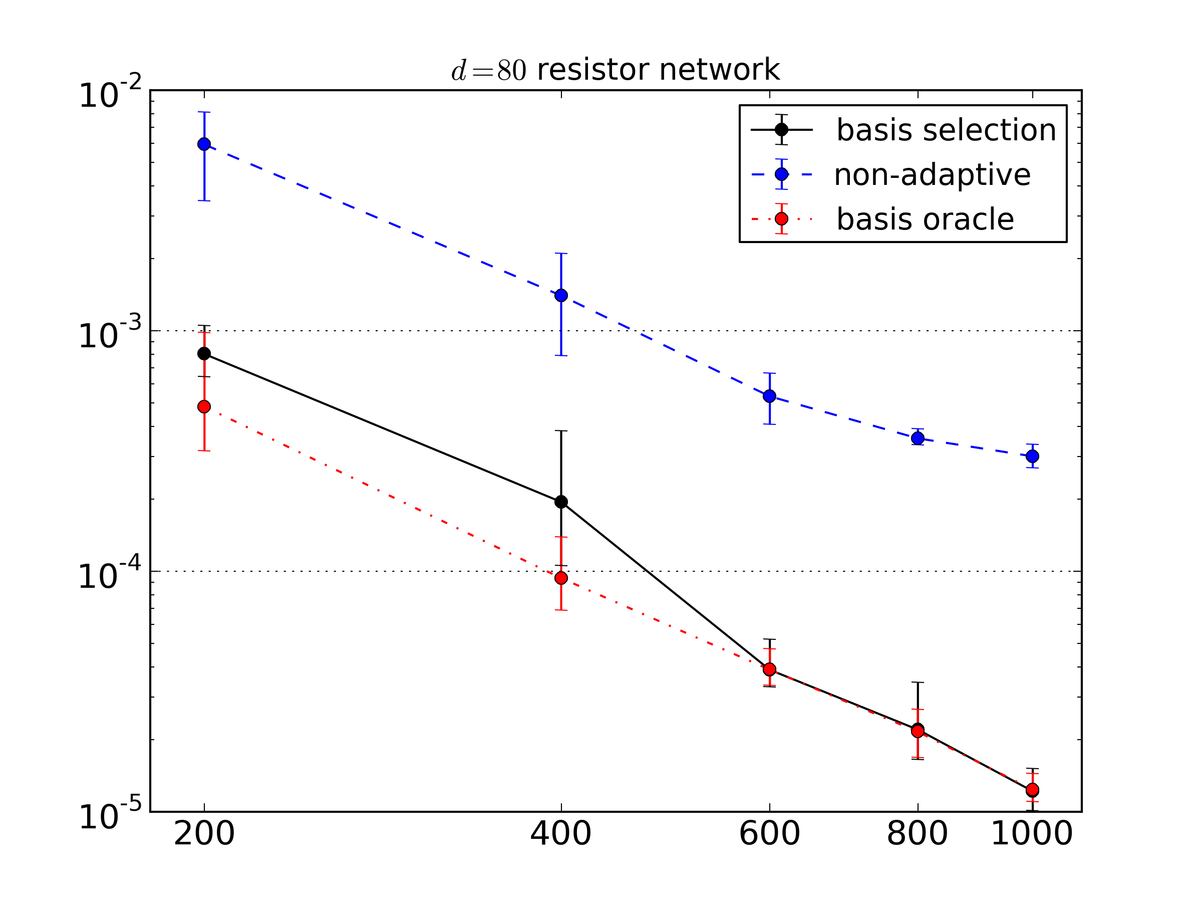
(b)

Figure 12: Convergence of the RMSE, with respect to increasing design size $M$, in the Legendre PCE approximation of the resistor network. The error bars represent the minimum and maximum error over the $20$ trials for each design size $M$.

5.5 Gradient-enhanced $\ell_{1}$-minimization

Typical $\ell_{1}$-minimization, when used for PCE approximation, attempts to find solutions to

$$\boldsymbol{\Phi}\boldsymbol{\alpha}\approx\mathbf{f}$$

where denotes the Vandermonde matrix with entries $\boldsymbol{\Phi}_{ij}=\phi_{j}({\boldsymbol{\xi}}_{i}),\quad i=1,\ldots,M,\;j=1,\ldots,N$. If gradients of the model $f$ with respect to the random variables ${\boldsymbol{\xi}}$ are known, then one can enhance the accuracy of the PCE by finding a solution to

$$\boldsymbol{\Phi}_{\partial}\boldsymbol{\alpha}\approx\mathbf{f}_{\partial}\quad\text{where}\quad\boldsymbol{\Phi}_{\partial}=\begin{bmatrix}\boldsymbol{\Phi}\\ {\frac{\partial\boldsymbol{\Phi}}{\partial\xi_{1}}}\\ \vdots\\ {\frac{\partial\boldsymbol{\Phi}}{\partial\xi_{d}}}\end{bmatrix},\quad\mathbf{f}_{\partial}\begin{bmatrix}\mathbf{f}\\ {\frac{\partial\mathbf{f}}{\partial\xi_{1}}}\\ \vdots\\ {\frac{\partial\mathbf{f}}{\partial\xi_{d}}}\end{bmatrix}$$

and $({\frac{\partial\boldsymbol{\Phi}}{\partial\xi_{n}}})_{ij}=\frac{\partial\phi_{j}}{\xi_{n}}({\boldsymbol{\xi}}_{i})$ and $(\frac{\partial\mathbf{f}}{\partial\xi_{n}})_{i}=\frac{\partial f}{\xi_{n}}({\boldsymbol{\xi}}_{i})$, $i=1,\ldots,M$, $j=1,\ldots,N$, $n=1,\ldots,d$. To find a solution we again use basis pursuit denoising and solve

$$\boldsymbol{\alpha}=\operatorname*{arg\,min}_{\boldsymbol{\alpha}}\;\|\boldsymbol{\alpha}\|_{1}\quad\text{such that}\quad\|\boldsymbol{\Phi}_{\partial}\boldsymbol{\alpha}-\mathbf{f}_{\partial}\|_{2}\leq\varepsilon$$

This gradient based formulation consists of $M(d+1)$ equations that match both function values and gradients, in comparison to (5) which consists of only $M$ equations that match function values.

Figure 13 demonstrates the utility of using gradient data to build PCE approximations of the corner-peak function (11) with $d=10$. Unlike the previous figures in this paper, the horizontal axis is no longer the number of model runs but rather the computational cost. We assume that running the model to only obtain function values costs one computational unit and running the model to obtain both function values and all gradients components requires two units. For example, adjoint methods for differential equations can be used to obtain all gradients at a cost less than or equal to the cost of one forward model run.

Despite the extra computational cost required to obtain gradients, the use of gradients improves both the PCE resulting from both the non-adaptive and basis selection methods. Similar to the results presented in Section 5.1 the results shown here demonstrate that basis selection is more accurate than the non-adaptive strategy. Again the relative benefit is dependent on the rate of decay of the PCE coefficients.

Basis selection is able to make effective use of gradient information. For a design $\boldsymbol{\Xi}$ with $M$ samples, the size of the gradient enhanced Vandermonde matrix is $M(d+1)\times N$. We see that for a given accuracy gradient-based PCE requires a factor of $4$ fewer samples than the PCE based on the function values only. This is close to the optimal reduction factor of $d/2=5$ that can be obtained using gradients, assuming that each gradient component is as informative as a function value and the cost of computing function values with gradients is twice the cost of just computing function values.

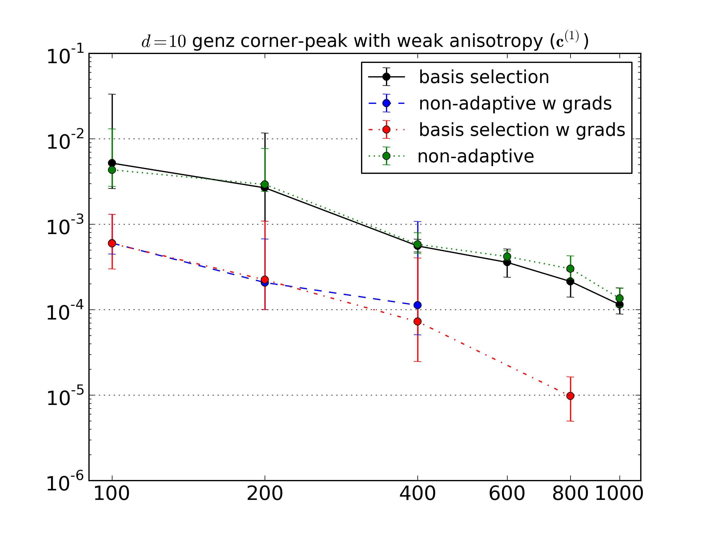
(a)

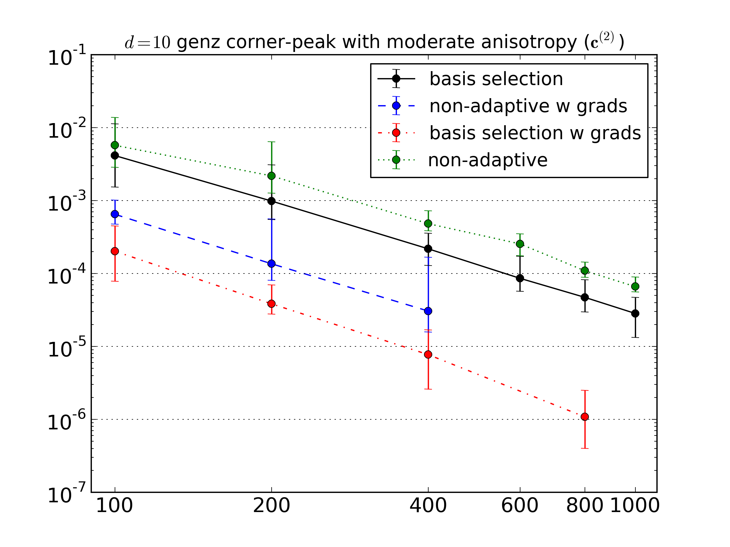
(b)

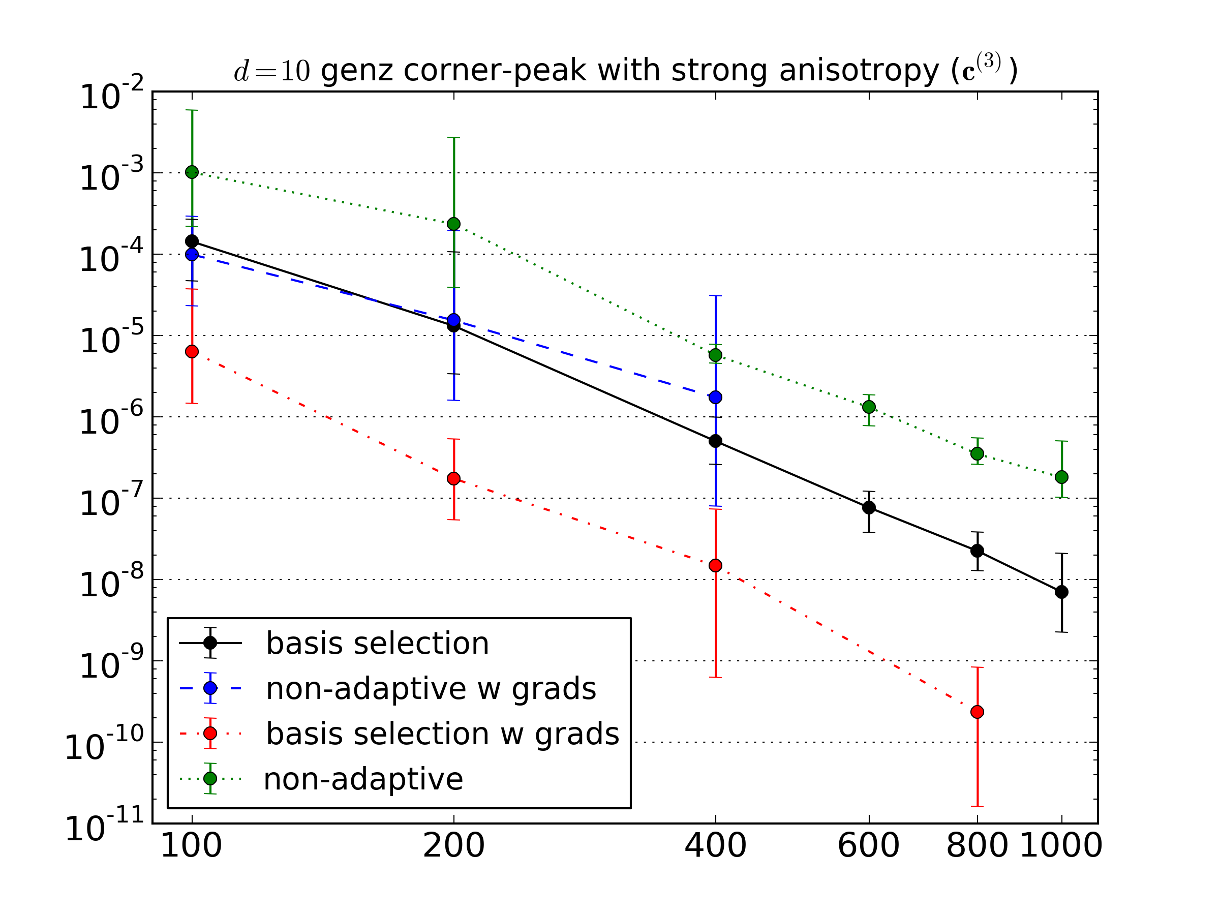
(c)

Figure 13: Convergence of the RMSE, with respect to increasing computation units, in the gradient-enhanced Legendre PCE approximation of the corner-peak function (11) for the three coefficient regimes: (a) $\mathbf{c}^{(1)}$, (b) $\mathbf{c}^{(2)}$, (c) $\mathbf{c}^{(3)}$. The error bars represent the minimum and maximum error over the $20$ trials for each design size $M$. We have assumed computing functional values at a design point is one unit and computing all gradient components is another unit. For example, the gradient enhanced basis selection approximation (dot-dash line) with 50 design points costs 100 units (horizontal axis value).

5.6 Non-uniform model inputs

Throughout this paper, we have discussed basis selection when applied to Legendre polynomials and uniform variables. However, basis selection can also be applied to other variable/polynomial combinations. Let us once again consider the resistor network, but now let ${\boldsymbol{\xi}}$ be Gaussian variables with mean $1.0$ and standard deviation $0.005.$ We now draw random samples from the aforementioned Gaussian distribution to form $\boldsymbol{\Xi}$ and run the model at each sample to obtain $f(\boldsymbol{\Xi})$. Figure 14 demonstrates that the advantages of basis selection are also present when we compute PCE approximations with non-uniform random variables.

Note that linear systems based upon Hermite polynomials suffer from poor numerical conditioning as the number of samples $M$ increases. This poor conditioning causes the non-monotone convergence shown. Development of sampling and pre-conditioning strategies for normal variables is an important area of future research, but is beyond the scope of this paper.

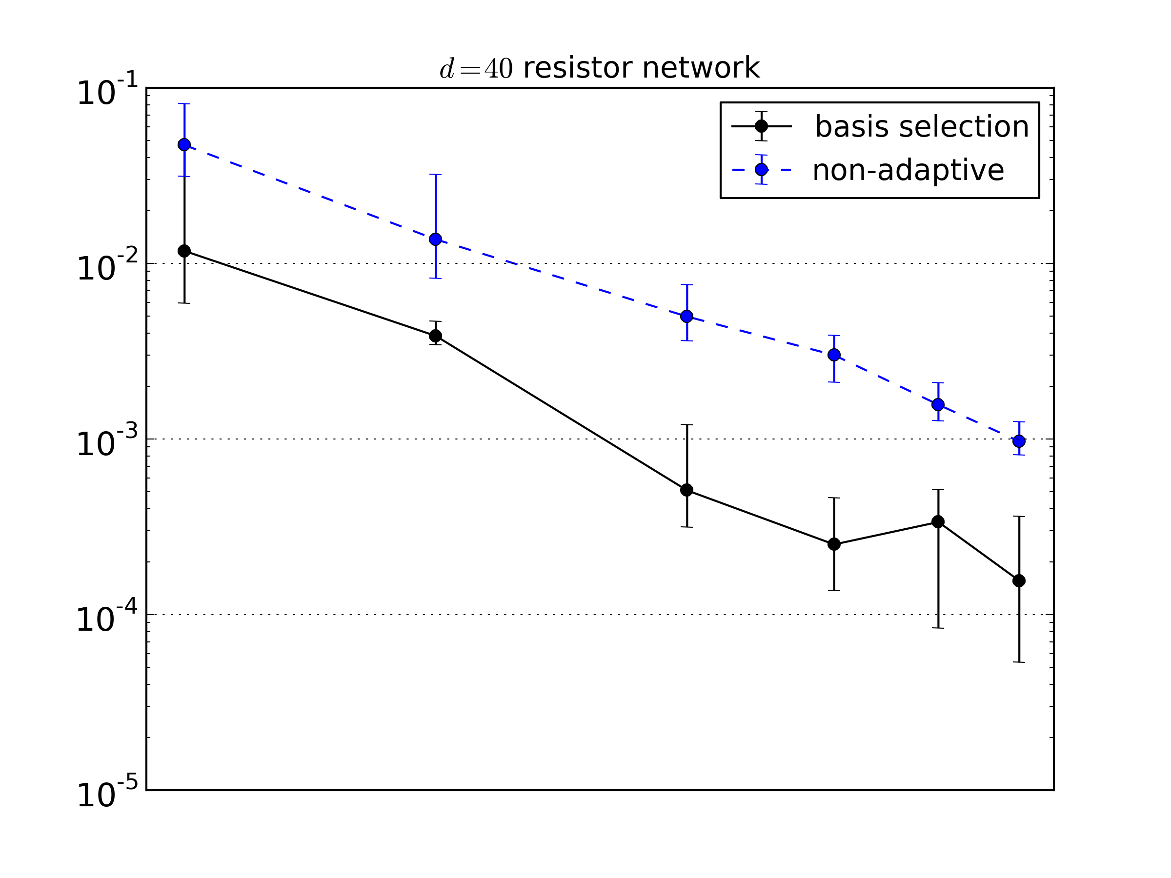
Figure 14: Convergence of the RMSE, with respect to increasing design size $M$, in the Hermite PCE approximation of the $d=40$ resistor network. The error bars represent the minimum and maximum error over the $20$ trials for each design size $M$.

6 Conclusions

In this paper we present a basis selection method that can be used with $\ell_{1}$-minimization to adaptively determine the large coefficients of polynomial chaos expansions (PCE). The method attempts to identify structure in the coefficients of a PCE and only applies $\ell_{1}$-minimization to those terms believed to have large coefficients. The adaptive construction produces anisotropic basis sets that have more terms in important dimensions and limits the number of unimportant terms which increase mutual coherence and thus degrade the performance of $\ell_{1}$-minimization. The basis selection method produces, for a given computational budget, a more accurate PCE than would be obtained if the basis is fixed a priori. The important features and the accuracy of basis selection are demonstrated with a number of numerical examples. Specifically we show that in high dimensions, for which high-order total-degree PCE bases are infeasible, basis selection allows accurate identification of high-order terms that cannot be captured by low-order total-degree expansions. We demonstrate that even for lower dimensional problems, for which high-order total-degree PCE bases are feasible, basis selection still produces more accurate results than basis sets that are fixed priori. Finally, we demonstrate that basis selection can effectively leverage function gradients and be applied to PCE of non-uniform random variables.

References

- [1] I. Babuska, R. Tempone, and G. Zouraris. Galerkin finite element approximations of stochastic elliptic partial differential equations. SIAM Journal on Numerical Analysis, 42(2):800–825, 2004.
- [2] I.M. Babuska, F. Nobile, and R. Tempone. A stochastic collocation method for elliptic partial differential equations with random input data. SIAM Journal on Numerical Analysis, 45(3):1005–1034, 2007.
- [3] R.G. Baraniuk, V. Cevher, M.F. Duarte, and C. Hegde. Model-based compressive sensing. Information Theory, IEEE Transactions on, 56(4):1982–2001, 2010.
- [4] J. Beck, R. Tempone, F. Nobile, and L. Tamellini. On the optimal polynomial approximation of stochastic pdes by galerkin and collocation methods. Mathematical Models and Methods in Applied Sciences, 22(09):1250023, 2012.
- [5] S. Becker, J. Bobin, and E. Candés. Nesta: A fast and accurate first-order method for sparse recovery. SIAM Journal on Imaging Sciences, 4(1):1–39, 2011.
- [6] Marcel Bieri and Christoph Schwab. Sparse high order {FEM} for elliptic spdes. Computer Methods in Applied Mechanics and Engineering, 198(13–14):1149 – 1170, 2009. {HOFEM07} International Workshop on High-Order Finite Element Methods, 2007.
- [7] Géraud Blatman and Bruno Sudret. Adaptive sparse polynomial chaos expansion based on least angle regression. Journal of Computational Physics, 230(6):2345 – 2367, 2011.
- [8] Petros Boufounos, Marco F. Duarte, and Richard G. Baraniuk. Sparse signal reconstruction from noisy compressive measurements using cross validation. In Statistical Signal Processing, 2007. SSP ’07. IEEE/SP 14th Workshop on, pages 299 –303, aug. 2007.
- [9] T.T. Cai and Lie Wang. Orthogonal matching pursuit for sparse signal recovery with noise. Information Theory, IEEE Transactions on, 57(7):4680–4688, July 2011.
- [10] Emmanuel J. Candes, Justin K. Romberg, and Terence Tao. Stable signal recovery from incomplete and inaccurate measurements. Communications on Pure and Applied Mathematics, 59(8):1207–1223, 2006.
- [11] S. Chen, D. Donoho, and M. Saunders. Atomic decomposition by basis pursuit. SIAM Rev., 43(1):129–159, January 2001.
- [12] A. Cohen, R. DeVore, and C. Schwab. Convergence rates of best n-term galerkin approximations for a class of elliptic spdes. Foundations of Computational Mathematics, 10(6):615–646, 2010.
- [13] Patrick R. Conrad and Youssef M. Marzouk. Adaptive smolyak pseudospectral approximations. SIAM J. Scientific Computing, 35(6), 2013.
- [14] P.G. Constantine, M.S. Eldred, and E.T. Phipps. Sparse pseudospectral approximation method. Computer Methods in Applied Mechanics and Engineering, 229–232(0):1–12, 2012.
- [15] D.L. Donoho, M. Elad, and V.N. Temlyakov. Stable recovery of sparse overcomplete representations in the presence of noise. Information Theory, IEEE Transactions on, 52(1):6–18, Jan 2006.
- [16] A . Doostan and H. Owhadi. A non-adapted sparse approximation of PDEs with stochastic inputs. Journal of Computational Physics, 230(8):3015 – 3034, 2011.
- [17] Marco F. Duarte, Michael B. Wakin, and Richard G. Baraniuk. Fast reconstruction of piecewise smooth signals from random projections. In Online Proceedings of the Workshop on Signal Processing with Adaptative Sparse Structured Representations (SPARS), Rennes, France, 2005.
- [18] J. Foo and G.E. Karniadakis. Multi-element probabilistic collocation method in high dimensions. J. Comput. Phys., 229(5):1536–1557, 2010.
- [19] B. Ganapathysubramanian and N. Zabaras. Sparse grid collocation schemes for stochastic natural convection problems. Journal of Computational Physics, 225(1):652–685, 2007.
- [20] A. Genz. A package for testing multiple integration subroutines. In P. Keas and G. Fairweather, editors, Numerical Integration, pages 337–340. D. Riedel, 1987.
- [21] R.G. Ghanem and P.D. Spanos. Stochastic Finite Elements: A Spectral Approach. Springer-Verlag New York, Inc., New York, NY, USA, 1991.
- [22] J.D. Jakeman and S.G. Roberts. Local and dimension adaptive stochastic collocation for uncertainty quantification. In Jochen Garcke and Michael Griebel, editors, Sparse Grids and Applications, volume 88 of Lecture Notes in Computational Science and Engineering, pages 181–203. Springer Berlin Heidelberg, 2013.
- [23] C. La and M.N. Do. Tree-based orthogonal matching pursuit algorithm for signal reconstruction. In Image Processing, 2006 IEEE International Conference on, pages 1277–1280, 2006.
- [24] X. Ma and N. Zabaras. An adaptive hierarchical sparse grid collocation algorithm for the solution of stochastic differential equations. Journal of Computational Physics, 228:3084–3113, 2009.
- [25] L Mathelin and KA Gallivan. A compressed sensing approach for partial differential equations with random input data. Commun. Comput. Phys., 12:919–954, 2012.
- [26] L. Mathelin, M. Hussaini, and T. Zang. Stochastic approaches to uncertainty quantification in CFD simulations. Numerical Algorithms, 38(1-3):209–236, MAR 2005.
- [27] Deanna Needell and Joel A. Tropp. Cosamp: Iterative signal recovery from incomplete and inaccurate samples. Commun. ACM, 53(12):93–100, December 2010.
- [28] F. Nobile, R. Tempone, and C.G. Webster. An anisotropic sparse grid stochastic collocation method for partial differential equations with random input data. SIAM Journal on Numerical Analysis, 46(5):2411–2442, 2008.
- [29] Carl Edward Rasmussen and Christopher K. I. Williams. Gaussian Processes for Machine Learning (Adaptive Computation and Machine Learning). The MIT Press, 2005.
- [30] Holger Rauhut and Rachel Ward. Sparse legendre expansions via -minimization. Journal of Approximation Theory, 164(5):517 – 533, 2012.
- [31] Khachik Sargsyan, Cosmin Safta, Habib N Najm, Bert J Debusschere, Daniel Ricciuto, and Peter Thornton. Dimensionality reduction for complex models via Bayesian Compressive Sensing. International Journal for Uncertainty Quantification, 4(1):63–93, 2014.
- [32] M. Tatang, W. Pan, R. Prinn, and G. McRae. An efficient method for parametric uncertainty analysis of numerical geophysical model. Journal of Geophysical Research, 102(D18):21925–21932, 1997.
- [33] R Tibshirani. Regression shrinkage and selection via the Lasso. Journal Of The Royal Statistical Society Series B-Methodological, 58(1):267–288, 1996.
- [34] E. van den Berg and M.P. Friedlander. Probing the pareto frontier for basis pursuit solutions. SIAM Journal on Scientific Computing, 31(2):890–912, 2008.
- [35] R. Ward. Compressed sensing with cross validation. Information Theory, IEEE Transactions on, 55(12):5773 –5782, dec. 2009.
- [36] D. Xiu and J.S. Hesthaven. High-order collocation methods for differential equations with random inputs. SIAM Journal on Scientific Computing, 27(3):1118–1139, 2005.
- [37] D. Xiu and G.E. Karniadakis. The Wiener-Askey Polynomial Chaos for stochastic differential equations. SIAM J. Sci. Comput., 24(2):619–644, 2002.
- [38] Z. Xu and T. Zhou. On sparse interpolation and the design of deterministic interpolation points. SIAM Journal on Scientific Computing, 2014. Accepted.
- [39] L. Yan, L. Guo, and D. Xiu. Stochastic collocation algorithms using -minimization. International Journal for Uncertainty Quantification, 2(3):279–293, 2012.
- [40] X. Yang and G.E. Karniadakis. Reweighted minimization method for stochastic elliptic differential equations. Journal of Computational Physics, 248(0):87 – 108, 2013.