Classical stochastic measurement trajectories: Bosonic atomic gases in an optical cavity and quantum measurement backaction

Abstract

We formulate computationally efficient classical stochastic measurement trajectories for a multimode quantum system under continuous observation. Specifically, we consider the nonlinear dynamics of an atomic Bose-Einstein condensate contained within an optical cavity subject to continuous monitoring of the light leaking out of the cavity. The classical trajectories encode within a classical phase-space representation a continuous quantum measurement process conditioned on a given detection record. We derive a Fokker-Planck equation for the quasi-probability distribution of the combined condensate-cavity system. We unravel the dynamics into stochastic classical trajectories that are conditioned on the quantum measurement process of the continuously monitored system, and that these trajectories faithfully represent measurement records of individual experimental runs. Since the dynamics of a continuously measured observable in a many-atom system can be closely approximated by classical dynamics, the method provides a numerically efficient and accurate approach to calculate the measurement record of a large multimode quantum system. Numerical simulations of the continuously monitored dynamics of a large atom cloud reveal considerably fluctuating phase profiles between different measurement trajectories, while ensemble averages exhibit local spatially varying phase decoherence. Individual measurement trajectories lead to spatial pattern formation and optomechanical motion that solely result from the measurement backaction. The backaction of the continuous quantum measurement process, conditioned on the detection record of the photons, spontaneously breaks the symmetry of the spatial profile of the condensate and can be tailored to selectively excite collective modes.

I Introduction

Studies of open interacting quantum many-body systems have recently attracted considerable interest. The coupled evolution of many-body systems with a large number of degrees of freedom and the environment leads to an interplay between the interactions and dissipation. This not only exhibits rich phenomenology but can also provide a platform for future applications of quantum technologies. Dissipation induces decoherence Joos and Zeh (1985); Zurek (2003); Walls and Milburn (1985); Leggett and Sols (1991), influences the correlations and dynamics Drummond and Corney (1999); Gardiner et al. (1998); Poletti et al. (2012); Ruostekoski and Walls (1998); Weiler et al. (2008); Khodorkovsky et al. (2009); Witthaut et al. (2009); Olmos et al. (2013); Pichler et al. (2010); Cockburn et al. (2010); Witthaut et al. (2011); Gilz and Anglin (2011); Höning et al. (2013), and engineering dissipative coupling may be employed in state preparation Syassen et al. (2008); Diehl et al. (2008); Jenkins and Ruostekoski (2012)

The backaction due to quantum measurement forms an essential ingredient of quantum physics. The evolution of a continuously monitored quantum system represents a coupling of the system to the environment where the dynamics is conditioned on the measurement outcome in each experimental run. Combining unitary quantum evolution with specifically designed measurements can be used to engineer desired quantum states–examples in many-atom systems include, e.g., preparation of spin squeezed atomic ensembles Leroux et al. (2010); Chen et al. (2011). The evolution of quantum states may be further influenced by implementing control and feedback mechanisms based on the measurement outcome Wiseman and Milburn (2010).

The evolution of a continuously monitored open quantum system may mathematically be expressed in terms of a master equation. The master equation can then represent the measurement outcome of ensemble-averaged quantities without revealing anything about how the measurement record of an individual experimental realization may behave. In order to express possible measurement records of individual experimental runs as a quantum stochastic process, an unconditioned master equation can be unraveled into stochastic quantum trajectories of state vectors (quantum Monte Carlo wave functions) Tian and Carmichael (1992); Dalibard et al. (1992); Dum et al. (1992). Each quantum trajectory is then conditioned on the measurement record and undergoes a series of stochastic ‘quantum jumps’, according to a given probability distribution. Each quantum trajectory produces a faithful simulation of an individual experimental realization, where a sequence of quantum jumps represents a possible measurement outcome, e.g., a photon count record on a detector, and the approach can also be extended to other detection schemes Carmichael (1993).

In practise, solving the dynamics of the entire master equation is numerically demanding and quantum trajectories work efficiently only for a small number of particles and for 2-3 quantum modes. However, in typical ultracold atom systems, for example, the interacting atom clouds form large spatially-dependent multimode quantum fields. In order to describe the quantum measurement-induced backaction in continuously observed ultracold atomic gases, one would therefore in general require numerically more efficient approximate approaches. It was recently shown in Ref. Javanainen and Ruostekoski (2013) for the case of a strongly interacting two-mode bosonic atomic gas confined in a double-well potential that the backaction of a continuous quantum measurement process can be approximately incorporated in a classical stochastic description. Furthermore, regarding the observed quantity, the classical representation of the quantum mechanical measurement backaction agrees with the full quantum solution: Even in a parameter regime where the unitary quantum dynamics in the absence of measurements cannot qualitatively be approximated by a classical stochastic representation, it was found that whenever continuous measurements are frequent enough to be able to resolve the dynamics, the measured observable behaves classically. In this context, we define classical dynamics as that which can be described by a valid classical probability distribution in phase-space and which conforms to classical logic. It is important to emphasize that many states with considerable quantum fluctuations, e.g., spin-squeezed systems belong to this category.

Here we formulate the notion of classical stochastic measurement trajectories to spatially-varying, interacting, multimode bosonic atomic systems. We consider a Bose-condensed atomic gas in a single-mode optical cavity where the light inside the cavity interacts with the condensate and the light leaking out of the cavity is continuously monitored. We construct the approximate Fokker-Planck equation for the system in the Wigner phase-space representation where we expand the full dynamical equation in terms of the interaction parameters that reflect the strength of many-body quantum fluctuations in the system. Constructing the classical measurement trajectories then follows the same principle as the formulation of quantum trajectories from the full quantum-mechanical master equation: We unravel the evolution of the Fokker-Planck equation into stochastic dynamical processes. Each trajectory then corresponds to the dynamics of the system conditioned on a single measurement record that represents a possible single, continuously monitored experimental run. The backaction of the measurement process is included classically as a dynamical noise term. When we ensemble-average over many such classical trajectories, we can reconstruct, within statistical uncertainty, the evolution of the Fokker-Planck equation.

By adiabatically eliminating the cavity photon field in the equations of motion for the atom-cavity system, we show that the measurements on the condensate in the classical limit are represented by a stochastic spatially-dependent diffusion term for the condensate phase profile that is determined by the cavity mode shape and pump profile. This results in phase patterns that considerably fluctuate between different measurement trajectories. In the ensemble averages over many such trajectories, we find that the effect of photons leaking out of the cavity is a spatially-varying phase decoherence rate. We also show that measurement backaction in individual trajectories can induce self-organization of a Bose-Einstein condensate (BEC) in an optical lattice. Each stochastic measurement trajectory leads to a characteristic evolution dynamics of the condensate phase profile and spatial density pattern for the atoms that is solely generated by a continuous quantum measurement process. The emergence of the density pattern represents a measurement-induced spontaneous symmetry breaking. Ensemble-averaging over many trajectories restores the initial uniform unbroken spatial pattern of atomic density. The randomly produced spatial pattern in a multimode BEC is related to the quantum-measurement induced relative phase between two single-mode BECs in quantum trajectory simulations Javanainen and Yoo (1996); Cirac et al. (1996); Castin and Dalibard (1997); Ruostekoski and Walls (1997): a measurement process can establish a well-defined relative phase between two BECs that initially possess no phase information–each measurement trajectory produces a random phase value and ensemble-averaging over many such runs wipes out the phase information, restoring the broken symmetry.

We show that the measurement process also leads to mechanical effects on the atoms, and we simulate the resulting optomechanical dynamics of a multimode condensate due to the continuous detection of the cavity mode, where the mechanical degrees of freedom are comprised by the coupled intrinsic collective excitations of the condensate. In this limit, where the condensate cannot be reduced to a single mode oscillator and subsequently exhibits rich dynamics, we show that it is nonetheless possible for the measurement to predominantly excite selected collective modes, such as the breathing mode. Tailoring the overlap of the condensate density and the cavity mode function tunes the nature of the measured quantity, and allows the selective coupling of a given collective mode. However, the multimode nature of the condensate can result in significant excitation of additional modes. For example, attempting to excite the center-of-mass mode leads to a substantial response of the breathing mode at later times.

Bose-condensed atomic gases confined in optical cavities provide ideal systems to study measurement backaction and the emergence of classicality by means of classical measurement trajectories. Ultracold atoms have proven to be capable of realizing controllable quantum systems with many degrees of freedom. Optical cavities, on the other hand, have enabled much work on the quantum nature of light and are a natural system to consider the effects of measurement on a single, or few, quantum modes Carmichael (1993, 2007). The union of the two, whereby an ultracold gas is placed inside an optical cavity, enables the study of the backaction of measurement on a multimode coupled quantum system. The cavity enhances the interaction of the light with the atoms, allowing the strong coupling regime to be reached Brennecke et al. (2007). The light imposes an optical potential on the atoms and the backaction of the continuous measurement of the cavity output on the dynamics of the atoms has been experimentally observed Murch et al. (2008); Brahms et al. (2012). The atoms, in turn, affect the resonance frequency of the cavity, and the motion of the atoms can then couple to the cavity field through the spatial variation of the atom-light coupling. The transfer of momentum between the cavity photons and the atoms also allows the realization of optomechanical systems–using the motion of BECs as a mechanical device coupled to the cavity light field Brennecke et al. (2008); Murch et al. (2008); Botter et al. (2013). In the case of atomic BECs, the optomechanical oscillator formed by the atoms is already in the ground state and does not need to be cooled by the cavity field–hence, the general challenge of cooling micro-mechanical oscillators in optomechanical applications can be circumvented in atomic systems.

Theoretical descriptions of these many-atom, many-mode systems have necessitated approximate treatments Ritsch et al. (2013). In the limit that excitations are small, the behavior of BECs in cavities may be approached by linearizing about a mean-field steady-state solution Horak and Ritsch (2001); Gardiner et al. (2001); Nagy et al. (2008); Szirmai et al. (2009); Kónya et al. (2011). Alternatively, the full multimode atomic field can be restricted to only one or two modes, allowing a more full quantum treatment Moore et al. (1999). With regards to measurement backaction, single atoms in optical cavities have been the subject of many quantum trajectory calculations Carmichael (1993); Ritsch et al. (2013). Semiclassical Niedenzu et al. (2013) and static discrete approximations Mekhov and Ritsch (2009) have been considered for larger atom clouds. Recently, an alternative phase-space treatment to the one presented in this paper was developed for a continuously monitored system that can incorporate a multimode approach and is also suitable for cavity systems Hush et al. (2013) (for an early development, see Szigeti et al. (2009)).

In the following Section, we introduce the full quantum theory of the cavity-BEC system, before discussing a phase-space representation suitable to describe our many-mode system in Sec. III. In Sec. IV we review the treatment of measurement backaction given by the theory of quantum trajectories, before showing that our classical phase-space picture can be unraveled to give classical measurement trajectories. We derive the corresponding classical trajectories for the coupled cavity-atom system, however, the effect of the measurement backaction on the atoms can more clearly be seen when the cavity field is adiabatically eliminated from the picture, as we show in Sec. V. In this picture, measurement of the light manifestly leads to stochastic evolution of the BEC phase profile, spatially modulated by the cavity mode and transverse pump profile. In Sec. VI we present numerical results illustrating the phase decoherence for a BEC in an optical lattice potential in an ensemble average over many stochastic trajectories, and show that the measurement backaction leads to self-organization or pattern formation. We show how the measurement backaction may be used in an optomechanical sense in Sec. VII, before discussing how stronger quantum fluctuations in the initial state can be included in Sec. VIII. Finally, in App. A we give a detailed treatment of the adiabatic elimination of the light used in Sec. V.

II Formalism

The Hamiltonian for a BEC in an optical cavity of frequency $\omega_{c}$ can be derived as a many-body extension of the Jaynes-Cummings Hamiltonian appropriate for a single two-level atom of resonance frequency $\omega_{a}$. After making a unitary transformation to the rotating frame of the pump, and using the rotating wave approximation, one then finds a second quantized Hamiltonian of the form  Jaynes and Cummings (1963); Walls and Milburn (1994); Maschler et al. (2008)

$$H_{ge}=H_{A}+H_{C}+H_{CA},$$ (1)

where

$$H_{A} =\int\mathrm{d}x\hat{\Psi}^{\dagger}_{g}(x)\left[-\frac{\hbar^{2}\nabla^{2}}{2m}+V_{g}(x)\right]\hat{\Psi}_{g}(x)$$

$$+\frac{U}{2}\int\mathrm{d}x\hat{\Psi}^{\dagger}_{g}(x)\hat{\Psi}^{\dagger}_{g}(x)\hat{\Psi}_{g}(x)\hat{\Psi}_{g}(x)$$

$$+\int\mathrm{d}x\hat{\Psi}^{\dagger}_{e}(x)\left[-\frac{\hbar^{2}\nabla^{2}}{2m}-\hbar\Delta_{pa}+V_{e}(x)\right]\hat{\Psi}_{e}(x)$$

$$-i\hbar\int\mathrm{d}x\left[\hat{\Psi}^{\dagger}_{g}(x)h(x)\hat{\Psi}_{e}(x)-\hat{\Psi}^{\dagger}_{e}(x)h(x)\hat{\Psi}_{g}(x)\right],$$ (2)

$$H_{CA} =-i\hbar\int\mathrm{d}x\hat{\Psi}^{\dagger}_{g}(x)g(x)\hat{a}^{\dagger}\hat{\Psi}_{e}(x)+\mbox{h.c.}\,,$$ (3)

$$H_{A} =-\hbar\Delta_{pc}\hat{a}^{\dagger}\hat{a}+i\hbar\eta(\hat{a}^{\dagger}-\hat{a})\,.$$ (4)

Here $\hat{\Psi}_{g(e)}(x)$ annihilates an atom in the ground (excited) state at position $x$, while $\hat{a}$ annihilates a photon from the single cavity mode of frequency $\omega_{c}$. The atoms and the cavity couple via the mode function

$$g(x)=g_{0}\sin(kx),$$ (5)

and the system can be pumped on the cavity axis at a rate $\eta$ or the atoms pumped directly from a transverse beam of profile $h(x)$. Interatomic interactions between atoms in the ground state are included via the contact interaction strength $U$, in 3D this would be $U_{3D}=4\pi\hbar^{2}a_{s}/m$, where $a_{s}$ is the $s$-wave scattering length, but we consider here the case that a tight trap of frequency $\omega_{\perp}$ constrains the dynamics to the single dimension along the cavity axis, leading to a 1D interaction strength $U_{1D}=2\hbar\omega_{\perp}a_{s}$. The remaining terms describe single particle atom motion in external traps $V_{g(e)}(x)$ affecting the ground (excited) state, and free evolution of the cavity field at a rate given by the detuning $\Delta_{pc}=\omega_{p}-\omega_{c}$. We note that the detuning between the pump and the atoms $\Delta_{pa}=\omega_{p}-\omega_{a}$ may in general be spatially dependent, but for brevity we will not normally include this dependence explicitly unless it is ambiguous.

In the limit that $\Delta_{pa}$ is large, then the excited state may be adiabatically eliminated from the equations of motion. The resulting effective Hamiltonian is

$$H_{1} =\int\mbox{d}x\hat{\Psi}^{\dagger}(x)\Bigg{\{}H_{0}+\frac{\hbar}{\Delta_{pa}}\bigg{[}h(x)^{2}+g(x)^{2}\hat{a}^{\dagger}\hat{a}$$

$$+h(x)g(x)\left(\hat{a}+\hat{a}^{\dagger}\right)\bigg{]}\Bigg{\}}\hat{\Psi}(x)$$

$$+\frac{U}{2}\int\mbox{d}x\hat{\Psi}^{\dagger}(x)\hat{\Psi}^{\dagger}(x)\hat{\Psi}(x)\hat{\Psi}(x)$$

$$-\hbar\Delta_{pc}\hat{a}^{\dagger}\hat{a}-i\hbar\eta\left(\hat{a}-\hat{a}^{\dagger}\right),$$ (6)

where $H_{0}=-\hbar^{2}/(2m)\nabla^{2}+V(x)$, and we drop the subscript indicating the atomic state since all atoms are assumed to be in the ground state. This effective Hamiltonian does not include the dissipative contribution of cavity photons lost through the cavity mirrors (we ignore spontaneous emission into modes not trapped in the cavity, which should be suppressed by the large detuning $\Delta_{pa}$ we have assumed).

In this work we are interested in a continuous quantum measurement process on the atom-light cavity system. We assume that all the photons leaked out of the cavity are detected on a photocounter of perfect efficiency. The detection rate is proportional to the cavity mode damping rate, which we model as $2\kappa$. The density operator for the coupled BEC and cavity system $\rho_{\mathrm{tot}}$ including the detection of the photons leaked out of the cavity then evolves according to the master equation

$$\frac{\partial\rho_{\mathrm{tot}}(t)}{\partial t}=-\frac{i}{\hbar}\left[H_{1},\rho_{\mathrm{tot}}(t)\right]+{\cal L}\rho_{\mathrm{tot}}(t),$$ (7)

where the Lindblad term Gardiner and Zoller (2004) incorporating the loss and measurement backaction is given by the superoperator ${\cal L}$, defined by

$${\cal L}\rho=\kappa\left(2\hat{a}\rho\hat{a}^{\dagger}-\hat{a}^{\dagger}\hat{a}\rho-\rho\hat{a}^{\dagger}\hat{a}\right).$$ (8)

However, such a master equation is not conditioned on any particular measurement record, but represents an ensemble average over a large number of measurement realizations, and as such describes the system when the measurement record is discarded. We discuss in Sec. IV how this master equation may be unraveled into trajectories conditioned on a given measurement record, however we first introduce a classical phase space description of the many-body problem.

III Classical phase-space picture

For the case of our many-atom many-mode system, the solution of the full quantum problem is numerically intractable, so here we turn to a treatment via classical phase space techniques, which we will later use to describe classical measurement trajectories. In quantum optics phase-space representations are a common technique for analyzing single and few mode quantum systems Walls and Milburn (1994); Gardiner and Zoller (2004). Here we represent the multimode atom-light system in terms of the Wigner function $W(\alpha,\alpha^{*},\{\psi,\psi^{*}\})$. The Wigner function has the role of a quasi-probability distribution, where $\alpha$ is the classical variable associated with $\hat{a}$ and $\psi$ is a classical field representation of the field operator $\hat{\Psi}$ that is stochastically sampled from an ensemble of Wigner distributed classical fields. The Wigner function has the property that expectation values of moments of classical variables correspond to symmetrically ordered expectation values of the corresponding quantum operators  Walls and Milburn (1994); Gardiner and Zoller (2004).

Multimode Wigner representations have been of great utility in studies of bosonic ultracold gases in closed systems Steel et al. (1998); Sinatra et al. (2002); Isella and Ruostekoski (2006); Blakie et al. (2008); Martin and Ruostekoski (2010); Polkovnikov (2010); Opanchuk and Drummond (2013) and can naturally include dissipation in open systems Walls and Milburn (1994); Gardiner and Zoller (2004), as has been investigated in the context of three-body losses Norrie et al. (2006a); Opanchuk and Drummond (2013). We derive below the equation of motion for the ensemble averaged quasi-probability distribution, before showing in the subsequent Section how individual classical measurement trajectories emerge from a mathematical correspondence to stochastic differential equations (SDEs). The equation of motion for this Wigner function is most easily obtained from the master equation (7) via the operator correspondences Gardiner and Zoller (2004); Walls and Milburn (1994) similar to

$$\hat{\Psi}\rho\leftrightarrow\left(\psi+\frac{1}{2}\frac{\delta}{\delta\psi^{*}}\right)W(\alpha,\alpha^{*},\{\psi,\psi^{*}\}),$$ (9)

leading to

$$\frac{\partial}{\partial t}W(\alpha, \alpha^{*},\{\psi,\psi^{*}\})=\int\mbox{d}x\frac{i}{\hbar}\frac{\delta}{\delta\psi}\Biggl{(}\Biggl{\{}H_{0}+\frac{\hbar}{\Delta_{pa}}\left[h(x)^{2}+g(x)^{2}\left(|\alpha|^{2}-\frac{1}{2}\right)+h(x)g(x)\left(\alpha+\alpha^{*}\right)\right]+U\left(|\psi|^{2}-1\right)\Biggr{\}}\psi W\Biggr{)}$$

$$+\frac{\partial}{\partial\alpha}\Biggl{(}\Biggr{\{}-\eta+(\kappa-i\Delta_{pc})\alpha+\frac{i}{\Delta_{pa}}\int\mbox{d}x\left(h(x)g(x)+g^{2}(x)\alpha\right)\left(|\psi(x)|^{2}-\frac{1}{2}\right)\Biggr{\}}W\Biggr{)}$$

$$+\frac{\kappa}{2}\frac{\partial^{2}}{\partial\alpha\partial\alpha^{*}}W$$

$$+\int\mbox{d}x\frac{i}{\hbar}\frac{U}{4}\frac{\delta^{3}}{\delta\psi^{2}\delta\psi^{*}}\psi W-\int\mbox{d}x\frac{i}{\Delta_{pa}}h(x)g(x)\frac{1}{4}\frac{\partial}{\partial\alpha}\frac{\delta^{2}}{\delta\psi\delta\psi^{*}}W$$

$$-\int\mbox{d}x\frac{i}{\Delta_{pa}}g^{2}(x)\Bigg{[}\frac{1}{4}\frac{\partial}{\partial\alpha}\alpha\frac{\delta^{2}}{\delta\psi\delta\psi^{*}}+\frac{1}{4}\frac{\delta}{\delta\psi}\psi\frac{\partial^{2}}{\partial\alpha\partial\alpha^{*}}\Bigg{]}W+\mbox{C.c.}\,.$$ (10)

If only the terms containing first and second order derivatives appeared in this expression, then they would form the drift and diffusion terms, respectively, of a Fokker-Planck equation for $W$. We will require a Fokker-Planck equation in order to argue that the evolution may be unraveled into individual classical stochastic trajectories in Sec IV.2. However, the appearance of the triple derivative terms in Eq. (10) prevents such an argument. These terms originate from the nonlinear atom-atom and atom-photon interaction terms in the master equation, which also give rise to drift terms. We argue below that, under appropriate conditions, the triple-derivative terms are small compared to the drift and diffusion terms and that we can neglect them.

We will analyze the leading order contributions of the interacting atom-light system in the limit of weak quantum fluctuations. The validity of the approximation is intrinsically linked to the basis representation used to simulate the system. Here we use a discrete spatial basis, discretized on a characteristic length scale $\ell$, and represent the stochastic field $\psi(x)$ by

$$\psi(x)=\sum_{i}\frac{1}{\sqrt{\ell}}\theta(x_{i}-\ell/2,x_{i}+\ell/2)a_{i},$$ (11)

where $\theta(x_{1},x_{2})$ is a rectangular function of unit amplitude and nonzero only between $x_{1}$ and $x_{2}$. The amplitudes $a_{i}$ can then be scaled by the number of atoms in the $i$th element $N_{i}$, by $\tilde{a}_{i}=a_{i}/\sqrt{N_{i}}$. The corresponding functional derivative operators are then

$$\frac{\delta}{\delta\psi(x)}=\sum_{i}\frac{1}{\sqrt{\ell N_{i}}}\theta(x_{i}-\ell/2,x_{i}+\ell/2)\frac{\partial}{\partial\tilde{a}_{i}}.$$ (12)

For the interparticle interaction we wish to investigate the scaling as we keep $C_{i}=N_{i}U$ constant, but take $N_{i}\rightarrow\infty$. Following an analogous motivation to treat the atom-photon interaction terms, we take the limit where the number of photons $n$ in the cavity tends to infinity while the maximum atom-photon interaction energy $\chi=\hbar(g_{0}^{2}/\Delta_{pa})n$ remains constant. We therefore, in addition to the rescaling of $\psi$ above, rescale $\tilde{\alpha}=\alpha/\sqrt{n}$ and replace $\hbar g_{0}^{2}/\Delta_{pa}$ by $\chi/n$. In order to reach this limit of large cavity photon number, we also note that the direct cavity pumping scales as $\eta\rightarrow\tilde{\eta}\sqrt{n}$, and include the spatial variation in the cavity coupling strength via $g(x)=g_{0}\tilde{g}(x)$. For the case of a transverse pumped system, motivated by the form of the transverse term in Eq. (6), we similarly keep $\chi_{h}=\hbar(h_{0}g_{0}/\Delta_{pa})\sqrt{n}$ constant, while photon number increases. For the spatial points where $N_{i}$ is large, the result of these substitutions is the equation of motion

$$\frac{\partial}{\partial\tilde{t}}\tilde{W}(\tilde{\alpha}, \tilde{\alpha}^{*},\{\tilde{a}_{i},\tilde{a}_{i}^{*}\})=i\sum_{i}\frac{\partial}{\partial\tilde{a}_{i}}\Biggl{(}\Biggl{\{}-\tilde{J}(\tilde{a}_{i+1}+\tilde{a}_{i-1})+\tilde{V}_{i}+\left[\tau_{0}\frac{\chi_{h}^{2}}{\chi}\tilde{h}_{i}^{2}+\tau_{0}\chi\tilde{g}^{2}_{i}\left(|\tilde{\alpha}|^{2}-\frac{1}{2}\frac{1}{n}\right)+\chi_{h}\tilde{h}_{i}\tilde{g}_{i}\left(\tilde{\alpha}+\tilde{\alpha}^{*}\right)\right]$$

$$+\frac{\ell^{2}}{\xi^{2}}\left(|\tilde{a}_{i}|^{2}-\frac{1}{N_{i}}\right)\Biggr{\}}\tilde{a}_{i}\tilde{W}\Biggr{)}+\frac{\partial}{\partial\tilde{\alpha}}\Biggl{(}\Biggr{\{}-\tilde{\eta}+(\tilde{\kappa}-i\tilde{\Delta}_{c})\tilde{\alpha}+i\sum_{i}\frac{N_{i}}{n}\left(\tau_{0}\chi_{h}\tilde{h}_{i}\tilde{g}_{i}+\tau_{0}\chi\tilde{g}^{2}_{i}\tilde{\alpha}\right)\left(|\tilde{a}_{i}|^{2}-\frac{1}{2}\frac{1}{N_{i}}\right)\Biggr{\}}\tilde{W}\Biggr{)}$$

$$+\frac{1}{n}\frac{\tilde{\kappa}}{2}\frac{\partial^{2}}{\partial\tilde{\alpha}\partial\tilde{\alpha}^{*}}\tilde{W}$$

$$+\frac{i}{4}\sum_{i}\frac{1}{N_{i}^{2}}\frac{\ell^{2}}{\xi^{2}}\frac{\partial^{3}}{\partial\tilde{a}_{i}^{2}\partial\tilde{a}_{i}^{*}}\tilde{a}_{i}\tilde{W}-\frac{i}{4}\sum_{i}\frac{1}{N_{i}n}\frac{\tau_{0}\chi_{h}}{\ell}\tilde{h}_{i}\tilde{g}_{i}\frac{\partial}{\partial\tilde{\alpha}}\frac{\partial^{2}}{\partial\tilde{a}_{i}\partial\tilde{a}_{i}^{*}}\tilde{W}$$

$$-\frac{i}{4}\sum_{i}\frac{1}{N_{i}n}\frac{\tau_{0}\chi}{\ell}\tilde{g}_{i}^{2}\frac{\partial}{\partial\tilde{\alpha}}\tilde{\alpha}\frac{\partial^{2}}{\partial\tilde{a}_{i}\partial\tilde{a}_{i}^{*}}\tilde{W}-\frac{i}{4}\sum_{i}\frac{1}{n^{2}}\frac{\tau_{0}\chi}{\ell}\tilde{g}^{2}_{i}\frac{\partial}{\partial\tilde{a}_{i}}\tilde{a}_{i}\frac{\partial^{2}}{\partial\tilde{\alpha}\partial\tilde{\alpha}^{*}}\tilde{W}+\mbox{C.c.}\,.$$ (13)

Here $\tilde{J}$ represents the tunneling between neighboring discrete sites and corresponds to the kinetic energy term in the continuum limit, and $\tilde{V}_{i},\tilde{g}_{i},\tilde{h}_{i}$ are spatially varying functions averaged over the width of the discrete basis states. We have also transformed to the dimensionless time scale $\tilde{t}=t/\tau_{0}$, with $\tau_{0}=(2m\ell^{2})/\hbar$, and so frequencies transform, for example, as $\tilde{\kappa}=\kappa\tau_{0}$. Several facts are now readily apparent. The tunneling and interaction energies are comparable when the width of the discrete basis states approaches the healing length $\xi=\hbar/\sqrt{2m\rho U}$, where $\rho$ is the 1D atomic density. The healing length represents the characteristic length scale associated with the nonlinear atom-atom interactions, and we set $\ell\approx\xi$. The first derivative (drift) terms can then be seen to all be independent of both the photon number and atom site occupation numbers in this scaling, with the exception of the constant $-1/2,-1$ terms introduced by nonlinear terms. Such constant corrections become negligible in the limit that the photon number and atom occupation numbers are large.

The diffusion term due to the continuous measurement of the cavity photon mode scales as $1/n$, since fluctuations become less important as the classical limit $n\rightarrow\infty$ is approached. However, the problematic triple derivative terms can all be seen to scale as $\epsilon_{i}^{2}$, $\epsilon_{n}^{2}$, or $\epsilon_{i}\epsilon_{n}$, where $\epsilon_{i}=1/N_{i}$ and $\epsilon_{n}=1/n$. Provided atom and photon numbers are large and so $\epsilon_{i,n}\ll 1$, we are therefore justified in neglecting the triple derivative terms, with the remaining drift and diffusion terms giving a Fokker-Planck equation.

So far we have considered regions where the atom number $N_{i}$ is large. In those spatial regions where $N_{i}$ is small, the atom-photon and atom-atom interactions provide negligible contributions to the system dynamics and these terms may be neglected in the original master equation. Therefore, no triple derivative terms occur for such regions.

Having neglected the triple derivative terms, we are left with a Fokker-Planck equation of the form

$$\frac{\partial}{\partial\tilde{t}}\tilde{W}= -\sum_{i}\frac{\partial}{\partial x_{i}}A_{i}({\bf{x}})\tilde{W}$$

$$+\frac{1}{n}\frac{\tilde{\kappa}}{2}\frac{\partial^{2}}{\partial\tilde{\alpha}\partial\tilde{\alpha}^{*}}\tilde{W}+\frac{1}{n}\frac{\tilde{\kappa}}{2}\frac{\partial^{2}}{\partial\tilde{\alpha}^{*}\partial\tilde{\alpha}}\tilde{W}\,,$$ (14)

where the index $x_{i}$ runs over the set $\big{\{}\tilde{\alpha},\tilde{\alpha}^{*},\{\tilde{a}_{i},\tilde{a}_{i}^{*}\}\big{\}}$. The matrix elements $A_{i}$ are given in the first two lines of Eq. (13), and these drift terms are responsible for the unitary Hamiltonian dynamics of the classical fields in the interacting atom-light cavity system. In contrast, the diffusion terms from the second line of Eq. (14) can be physically associated with the continuous measurement of the intensity of light leaking from the cavity. These terms represent a continuous quantum measurement process on the coupled atom-light system. For clarity, we now revert to the continuum limit, with the implicit assumption that the resulting equations will be solved on a discrete grid satisfying the above criteria.

In order to derive a Fokker-Planck equation for the atom-light system, we have kept the leading order terms in the limit of weak quantum fluctuations. The expansion is done with respect to both the nonlinear interparticle interaction and the atom-light coupling strength. In the case of the nonlinear $s$-wave interaction $U$ the requirement of weak quantum fluctuations becomes clear when we observe that the condition $N_{i}\gg 1$ can be related to the 1D Tonks parameter $\gamma=mU/(\hbar^{2}n)$. The Tonks parameter measures the ratio of the nonlinear $s$-wave interaction to kinetic energies for atoms spaced at the mean interatomic distance, and the number of atoms found in a length $\ell\simeq\xi$ is $N_{\xi}\simeq 1/\sqrt{2\gamma}$. (In contrast, in 3D the result is $N_{\xi}=1/(2\gamma_{3D})^{3/2}$, where $\gamma_{3D}=m\rho_{3D}^{1/3}U_{3D}/\hbar^{2}$ is again the ratio of interaction energy to kinetic energy.) The expansion therefore is strictly valid in the $\gamma\ll 1$ regime, that of a weakly interacting bosonic gas, although especially in 1D systems short-time behavior can be qualitatively described even for more strongly fluctuating cases Ruostekoski and Isella (2005). In the classical weakly fluctuating limit $N\rightarrow\infty$, $U\rightarrow 0$, with $NU=C$ kept constant, the Bogoliubov approximation becomes accurate and eventually one recovers the Gross-Pitaevskii mean-field theory Ruostekoski and Isella (2005). However, as we will argue in Sec. IV, in a continuously monitored system, when an observable is sufficiently accurately resolved in a detection process, it starts behaving classically even deep in the quantum regime. Therefore, regarding the dynamics of a frequently measured observable, the classical phase-space theory is expected to describe approximately even cases with strong quantum fluctuations.

The derivation of a Fokker-Planck equation is reminiscent of dropping the triple derivative terms that arise from the $s$-wave interactions in the truncated Wigner approximation Steel et al. (1998); Sinatra et al. (2002); Norrie et al. (2006b); Isella and Ruostekoski (2006); Blakie et al. (2008); Martin and Ruostekoski (2010); Polkovnikov (2010); Opanchuk and Drummond (2013) for a closed bosonic atomic system. While we have used a discrete spatial basis argument here, similar arguments for truncating the interparticle interactions have been made using spectral basis decompositions Norrie et al. (2006b); Opanchuk and Drummond (2013). When using the truncated Wigner method it is common to neglect the constant term introduced by the interparticle interactions, letting $(|\psi|^{2}-1)\rightarrow|\psi|^{2}$, since it leads only to a spatially constant phase rotation. We note that here [see Eq. (13)] the comparable terms introduced by the atom-light couplings are spatially varying and cannot trivially be neglected.

Equation (14) describes the evolution of the phase-space distribution $W(\alpha,\alpha^{*},\{\psi,\psi^{*}\})$ unconditioned on any particular measurement trajectory. As such, it corresponds to an approximation to the evolution given in a full quantum treatment by the master equation (7), ensemble averaged over all possible measurement outcomes. We wish to study the backaction due to a particular measurement record, and so turn to a decomposition of the problem into classical measurement trajectories representing individual experimental runs. In the following Section, we first discuss the case in the fully quantum limit, before showing that our Fokker-Planck equations can be unraveled to give classical descriptions for a continuously monitored atom-cavity system.

IV Conditioned measurement trajectories

IV.1 Quantum trajectories

For a system with Hamiltonian $H$, the quantum-mechanical evolution of the density matrix is given by the master equation

$$\dot{\rho}=-\frac{i}{\hbar}\left[H,\rho\right]+{\cal L}\rho\,.$$ (15)

Here we assume that the system is continuously monitored and the generic measurement process is represented by the coupling to the environment that exhibits the Lindblad form

$${\cal L}\rho=2\hat{A}\rho\hat{A}^{\dagger}-\hat{A}^{\dagger}\hat{A}\rho-\rho\hat{A}^{\dagger}\hat{A}\,.$$ (16)

The ensemble averaged behavior of the density matrix can be unraveled into stochastic quantum trajectories of state vectors (quantum Monte Carlo wave functions) Dalibard et al. (1992); Dum et al. (1992); Tian and Carmichael (1992). Each trajectory then corresponds to the dynamics of the system conditioned on a single measurement record and represents a stochastic process. Averaging over many such trajectories reproduces the results of the unconditioned master equation, complete with the correct statistics for the measured quantity, within statistical uncertainty.

In the limit that individual measurement events (such as photon emissions) can be resolved, the trajectories have the form of a series of quantum jumps Dalibard et al. (1992); Dum et al. (1992); Tian and Carmichael (1992), with individual counting events occurring at discrete random times which conform to the relevant probability distribution. The above Lindblad term represents a system in which the density operator changes by $\rho\rightarrow 2\hat{A}\rho\hat{A}^{\dagger}$ when a measurement (a ‘jump’) is made. So, for a system in a pure state, when a measurement occurs during a given small time-step, the wavefunction changes by

$$|\psi_{\mathrm{sys}}(t+\Delta t)\rangle=\sqrt{2}\hat{A}|\psi_{\mathrm{sys}}(t)\rangle,$$ (17)

and the wavefunction must then be renormalized.

In contrast, between jumps the absence of measurement clicks on a detector also conveys information about the system, and this backaction can be included by evolving the wavefunction with the nonunitary Hamiltonian $H-i\hbar\hat{A}^{\dagger}\hat{A}$. The times at which jumps occur are given by comparing the loss of norm due to the nonunitary evolution with a number chosen randomly from a uniform distribution between $0$ and $1$, which ensures the correct measurement statistics are reproduced. For a system which is sufficiently small that such an evolution is computationally feasible, a quantum trajectory can be simulated that includes the backaction due to a particular measurement record. That record is given by the set of discrete times at which the quantum jumps have occurred. In the limit of a large rate of photon emissions such that individual emissions are not resolved, but that the measurement is instead of a continuous flow of photons, the quantum stochastic trajectories become SDEs for the state vector of the system Carmichael (1993, 2007); Wiseman and Milburn (2010).

Such quantum trajectories are beyond our current ability to numerically simulate when the number of modes becomes large. Fortunately, as we will show in the following Section, the classical phase-space picture we developed (Sec. III) can be unraveled in an analogous manner, and provides a natural approximate description for single experimental runs subject to cavity light measured outside of the cavity.

IV.2 Measurement trajectories in a classical phase-space picture

In Sec. III we derived an approximate representation for the continuously monitored atom-cavity system in the form of a Fokker-Planck equation. In the resulting description (14) the nonlinear atom-light dynamics is incorporated in the drift term and the backaction of the continuous quantum measurement process, whereby photons leak out of the cavity and are continuously monitored by light intensity measurements, constitutes the diffusion part of the equation. This Fokker-Planck equation for the ensemble averaged quasi-probability distribution $W(\alpha,\alpha^{*},\{\psi,\psi^{*}\})$ can then be mathematically mapped onto systems of SDEs Gardiner and Zoller (2004); Carmichael (2010).

For our coupled BEC and cavity system, in the weakly fluctuating limit, the resulting coupled Ito SDEs that follow from the Fokker-Planck equation read

$$i\hbar\frac{\partial}{\partial t}\psi(x,t) =\biggl{\{}-\frac{\hbar^{2}}{2m}\nabla^{2}+V(x)+U|\psi|^{2}$$

$$+\frac{\hbar}{\Delta_{pa}}\bigg{[}h(x)^{2}+g(x)^{2}\left(|\alpha|^{2}-\frac{1}{2}\right)$$

$$+h(x)g(x)\left(\alpha+\alpha^{*}\right)\bigg{]}\biggr{\}}\psi,$$ (18)

$$d\alpha =\bigg{[}\eta-\kappa\alpha+i\left(\Delta_{pc}-\frac{1}{\Delta_{pa}}\int\mbox{d}xg^{2}(x)|\psi(x)|^{2}\right)\alpha$$

$$-\frac{i}{\Delta_{pa}}\int\mbox{d}xh(x)g(x)|\psi(x)|^{2}\bigg{]}\mathrm{d}t$$

$$+\sqrt{\frac{\kappa}{2}}\left(\mathrm{d}W_{x}+i\mathrm{d}W_{y}\right),$$ (19)

where $\mathrm{d}W_{x,y}$ are two independent Wiener increments satisfying $\langle\mathrm{d}W_{i}\rangle=0$, $\langle\mathrm{d}W_{i}^{2}\rangle=\mathrm{d}t$, and $\langle\mathrm{d}W_{i}\mathrm{d}W_{j}\rangle=0$. We have neglected here terms in Eq. (18) which lead merely to overall phase rotation of the stochastic field $\psi(x,t)$.

According to this mapping, the diffusion term in the Fokker-Planck equation represents a dynamical noise term in the corresponding SDE. The noise term has a physical origin resulting from the backaction of a continuous quantum measurement process in which the intensity of light leaking out of the cavity monitored. For simplicity, we assume a perfect photon detection process where every photon escaping the cavity is measured. In each individual realization of the stochastic dynamics, determined by Eqs. (18) and (19), the evolution is therefore conditioned on a particular continuous measurement record that directly corresponds to the classical approximation of an individual experimental run. The measurement backaction on atomic BECs becomes even more evident in next Section when we adiabatically eliminate the cavity field and the continuously observed quantity is expressed in terms of the atomic fields.

We have constructed the classical stochastic measurement trajectories by unraveling the evolution of the Fokker-Planck equation into stochastic dynamical processes in such a way that the stochastic noise term in each realization corresponds to a particular measurement record on a detector. The method uses a similar principle to the formulation of quantum trajectories of stochastic state vectors from the full quantum-mechanical master equation. Each individual classical trajectory is a faithful representation of a possible single experimental run of a continuous detection record. The behavior of the Fokker-Planck equation, unconditioned on any particular measurement record, and quantum-mechanical ensemble averages of the observed quantities can be reconstructed from an ensemble average over many individual trajectories. In this classical approximation individual discrete counting events of the photons can no longer be resolved in the noise contribution that approximates a continuous stream of photons.

For a given trajectory solution, the corresponding measurement record is that of photon counts occurring at the rate $r_{\mathrm{meas}}(t)=2\kappa(|\alpha(t)|^{2}-1/2)$. The remaining terms in Eq. (19) give the Hamiltonian evolution of the cavity mode variable, which couples to the atoms through a transverse pumping term and through a density dependent resonance shift. Similarly, the terms in Eq. (18) represent the Hamiltonian evolution of the atoms, with familiar terms for the dynamics of a BEC in a trap, extra terms due the dipole potential from the cavity and transverse pump light fields, proportional to $g^{2}(x)$ and $h^{2}(x)$ respectively, and a term describing the scattering process whereby an atom absorbs a photon from the transverse beam and emits into the cavity mode.

We emphasize here, that in this paper we use “classical” dynamics to mean that which can be described by a valid classical probability distribution in phase-space and which conforms to classical logic. Several interacting many-body systems with significant quantum fluctuations belong to this category, e.g., spin squeezed states Gross et al. (2011); Cattani et al. (2013).

To accurately represent a single experimental realization the initial conditions must be chosen with care. In practice, they can be sampled stochastically from the quasi-probability density $W(\alpha,\alpha^{*},\{\psi,\psi^{*}\},t=0)$ in a manner to reproduce as accurately as possible, or desirable, the correct quantum statistical correlations for the system. We address this further in Sec. VIII.

In the stochastic representation $W(\alpha,\alpha^{*},\{\psi,\psi^{*}\},t=0)$ is chosen as a valid classical probability distribution for the initial state, even though quantum fluctuations (such as mode squeezing) are approximately included. The approximate Fokker-Planck equation (14) for the atom-light system preserves the validity of the classical probabilistic description. Equation (14) also includes the quantum measurement backaction into the evolution of the quasi-probability density. The decomposition of the Fokker-Planck equation into SDEs then incorporates measurements into our classical trajectories.

For a continuously monitored strongly interacting two-mode system of bosonic atoms in a double-well potential, it was shown that such classical measurement trajectories agreed with the exact quantum solutions even in the limit of strong quantum fluctuations for observables whose dynamics were well resolved by the measurement Javanainen and Ruostekoski (2013). By using two detectors to measure the photons coherently scattered from an off-resonant source by atoms in each well, the populations of the two wells were continuously monitored and the population difference $z(t)$ between the wells could be inferred. When the measurement rate was high enough to allow the resolution of the dynamics of $z(t)$–a measurement rate as low as $10$ photons per characteristic oscillation period of $z(t)$–it was shown that the classical trajectories agreed with the quantum trajectories. This agreement held even for systems with as few as $10$ atoms, deep in what would normally be considered a quantum regime. The example demonstrates more generally how classical physics emerges from quantum mechanics as a result of the backaction of a continuous quantum measurement process. We may conjecture that in few- or many-body systems any continuously measured observable whose dynamics is resolved by a sufficiently frequent measurement rate can be closely approximated by classical dynamics. In other words, although the mathematical derivation of the approximate Fokker-Planck equation (14) relies on the assumption of weak quantum fluctuations, the dynamics could therefore be approximately predicted by the classical formalism for any continuously measured observable that is resolved by a sufficiently frequent detection rate, even when the system is strongly fluctuating. It was argued in Ref. Javanainen and Ruostekoski (2013) that this emergent classicality via continuous measurement is a consequence of the suppression of quantum interference effects that results from measurement backaction Walls and Milburn (1985).

V Measurement backaction on atoms - adiabatically eliminating the cavity mode

While Eqs. (18) and (19) are numerically tractable and can be solved directly, if we wish to consider the effect of the measurement on the atoms we can gain some insight by adiabatically eliminating the cavity light mode.

We give here a heuristic explanation of the derivation, and leave a more rigorous derivation to Appendix A. The equation of motion for $\hat{a}$ obtained from Eq. (6) is

$$\frac{\mathrm{d}{\hat{a}}}{\mathrm{d}t} =\left(i\left[\Delta_{pc}-\frac{1}{\Delta_{pa}}\int\hat{\Psi}^{\dagger}(x)\hat{\Psi}(x)g^{2}(x)\mathrm{d}x\right]-\kappa\right)\hat{a}$$

$$+\eta-\frac{i}{\Delta_{pa}}\int\hat{\Psi}^{\dagger}(x)\hat{\Psi}(x)h(x)g(x)\mathrm{d}x,$$

and in the bad cavity limit ($\kappa\gg g_{0}$) we eliminate the field by setting

$$\hat{a}=\frac{1}{\kappa-i\tilde{\Delta}_{pc}}\left(\eta-\frac{i}{\Delta_{pa}}\int\hat{\Psi}^{\dagger}(x)\hat{\Psi}(x)h(x)g(x)\mathrm{d}x\right).$$ (21)

Here $\tilde{\Delta}_{pc}=\Delta_{pc}-(1/\Delta_{pa})\int\hat{\Psi}^{\dagger}(x)\hat{\Psi}(x)g^{2}(x)\mathrm{d}x$ incorporates the atomic density resonance shift into the detuning. In order to make the transformation to the Wigner function picture tractable, we remove the atom contribution from the denominator by expanding in terms of the small parameter $\tilde{\Delta}_{pc}/\kappa$, leading to

$$\hat{a} =\frac{1}{\kappa}\left(\eta-\frac{i}{\Delta_{pa}}\int\hat{\Psi}^{\dagger}(x)\hat{\Psi}(x)h(x)g(x)\mathrm{d}x\right)$$

$$\times\left(1+i\frac{\tilde{\Delta}_{pc}}{\kappa}+O\left(\frac{\tilde{\Delta}_{pc}^{2}}{\kappa^{2}}\right)\right).$$ (22)

To further reduce the complexity of the equations, we now specialize below to the case of a cavity pumped solely on axis. Later we consider the case of the transversely pumped system.

V.1 Axially pumped cavity

If there is no transverse pumping of the atoms ($h(x)=0$), then eliminating the cavity field operator leads to a master equation for the atoms

$$\frac{\partial\rho_{a}(t)}{\partial t}=-\frac{i}{\hbar}\left[H_{2},\rho_{a}(t)\right]+{\cal L}\rho_{a}(t).$$ (23)

To the lowest order in our expansion parameter, the Hamiltonian part is

$$H_{2} =\int\mbox{d}x\hat{\Psi}^{\dagger}(x)\Bigg{[}-\frac{\hbar^{2}}{2m}\nabla^{2}+V(x)$$

$$+\frac{U}{2}\hat{\Psi}^{\dagger}(x)\hat{\Psi}(x)+\hbar\frac{|\eta|^{2}}{\kappa^{2}}\frac{g^{2}(x)}{\Delta_{pa}}\Bigg{]}\hat{\Psi}(x).$$ (24)

Similarly, the Lindblad term becomes to this order

$${\cal L}\rho_{a}=\frac{|\eta|^{2}}{\kappa^{3}}\left(2\hat{X}\rho_{a}\hat{X}-\hat{X}\hat{X}\rho_{a}-\rho_{a}\hat{X}\hat{X}\right),$$ (25)

where the operator $\hat{X}$ is used to represent

$$\hat{X}=\int\mathrm{d}x\frac{g^{2}(x)}{\Delta_{pa}}\hat{\Psi}^{\dagger}(x)\hat{\Psi}(x).$$ (26)

In contrast to the earlier results, now the measurement observable depends solely on atomic operators. From a quantum trajectory viewpoint, each photon measurement causes a change in the density matrix due to the jump operator

$${\cal J}\rho_{a}=\frac{2|\eta|^{2}}{\kappa^{3}}\hat{X}\rho_{a}\hat{X}.$$ (27)

The measurement of the intensity of light lost from the cavity can then be seen to give a measure of the squared integrated density of the atoms, modulated by the cavity mode shape and any spatial dependence of the detuning. The probability for such a loss event in a short time $\delta t$ is $\mathrm{Tr}\{{\cal J}\rho_{a}\delta t\}$, and so the rate of scattered photons counted by the measurement apparatus is

$$r_{\mathrm{meas}}(t)=\frac{2|\eta|^{2}}{\kappa^{3}}\langle\hat{X}\hat{X}\rangle.$$ (28)

In this adiabatic eliminated formalism, the measurement operator involves an integral over a nonuniform multimode quantum field $\hat{\Psi}(x)$ combined with a spatially varying cavity coupling strength. The motivation for our classical measurement trajectories is particularly clear in this picture, since the full quantum trajectory approach for such a measurement operator is not numerically feasible, with the exception of limiting cases where the atoms may be simplified to very few modes. In the following numerical examples we simulate measurement backaction on a spatial grid of the order of 1000 points. Therefore, we again use a classical Wigner representation, but having eliminated the cavity field we can now use a representation in terms solely of the atomic variables $W(\{\psi(x),\psi(x)^{*}\})$. However, before we give the full expression for the resulting classical trajectories, the effect of the measurement terms can be more transparently demonstrated by using a density and phase basis. Defining $\psi(x)=f(x)\exp(i\Phi(x))$, such that $f^{2}(x)$ corresponds to the density of the atoms and $\Phi(x)$ the phase, we express the Wigner function equation of motion for $W(\{f(x),\Phi(x)\})$. Momentarily concerning ourselves solely with the contribution from the measurement terms in the master equation, the following terms appear in the Fokker-Planck equation

$$\left.\frac{\partial}{\partial t}W(\{f(x),\Phi(x)\})\right|_{\mathrm{meas.}}=\int\mathrm{d}x\Bigg{[}2\frac{|\eta|^{2}}{\kappa^{2}}\frac{g^{2}(x)}{\Delta_{pa}(x)}\frac{\delta}{\delta\Phi(x)}\\ +\frac{1}{2}\int\mathrm{d}x^{\prime}2\frac{|\eta|^{2}}{\kappa^{3}}\frac{g^{2}(x)g^{2}(x^{\prime})}{\Delta_{pa}(x)\Delta_{pa}(x^{\prime})}\frac{\delta^{2}}{\delta\Phi(x)\delta\Phi(x^{\prime})}\Bigg{]}W.$$ (29)

The measurement part of this Fokker-Planck equation has a positive semidefinite diffusion matrix and can be mapped onto the SDEs

$$\left.\frac{\mathrm{d}f(x)}{\mathrm{d}t}\right|_{\mathrm{meas.}} = 0,$$ (30)

$$\left.\mathrm{d}\Phi(x)\right|_{\mathrm{meas.}} = \sqrt{2}\frac{|\eta|}{\kappa^{3/2}}\frac{g^{2}(x)}{\Delta_{pa}(x)}\mathrm{d}W,$$ (31)

where $\mathrm{d}W$ is a single Wiener increment with $\langle\mathrm{d}W\rangle=0$, $\langle\mathrm{d}W^{2}\rangle=\mathrm{d}t$. The measurement can be seen not to cause any direct dynamics of the density of the atoms, but instead to lead to a stochastic evolution of the phase profile that can considerably fluctuate between different measurement trajectories. This phase noise is spatially dependent, due to the cavity mode shape and any variation in the detuning. When we ensemble average over many such measurement trajectories, the fluctuating phase in different trajectories results in phase decoherence. The ensemble averaged evolution is no longer conditioned on any particular measurement record, and within statistical uncertainty approximates the evolution of the corresponding Fokker-Planck equation.

Including the Hamiltonian terms from Eq. (24), and reverting to the $\psi(x)$ representation, the Fokker-Planck equation for the atomic Wigner function can be unraveled into classical trajectories obeying

$$\mathrm{d} \psi(x)=\Bigg{\{}\frac{-i}{\hbar}\left[H_{0}+U|\psi(x)|^{2}\right]-i\frac{|\eta|^{2}}{\kappa^{2}}\frac{g^{2}(x)}{\Delta_{pa}(x)}F$$

$$-\frac{|\eta|^{2}}{\kappa^{3}}\frac{g^{4}(x)}{\Delta_{pa}^{2}(x)}\Bigg{\}}\psi(x)\mathrm{d}t-i\sqrt{2\frac{|\eta|^{2}}{\kappa^{3}}}\frac{g^{2}(x)}{\Delta_{pa}(x)}\psi(x)\mathrm{d}W.$$ (32)

The first term corresponds to the normal nonlinear evolution of the atoms in the absence of light or the cavity. For the lowest order expansion in our small parameter, we have $F\approx 1+O(\tilde{\Delta}_{pc}/\kappa)$, and so the second term includes the effects of the optical potential due to a standing wave of light in the cavity. The more rigorous derivation given in Appendix A provides a higher order term

$$F\approx\left[1+\frac{\Delta_{pc}}{\kappa^{2}}\int\frac{g^{2}(x^{\prime})}{\Delta_{pa}(x^{\prime})}|\psi(x^{\prime})|^{2}\mathrm{d}x^{\prime}\right]+O\left[\left(\frac{\tilde{\Delta}_{pc}}{\kappa}\right)^{2}\right],$$ (33)

which includes interactions between atoms mediated by cavity photon exchange and can be understood as a change in the cavity resonance frequency due to the distribution of the atoms. The two terms on the second line (32) both arise from the measurement process, and together result in the stochastic phase evolution of Eq. (31). Note that while neither of the measurement terms appear to conserve particle number in this representation, the sum of the two terms does do so, as indicated by Eq. (30).

V.2 Transversely pumped atoms

In contrast, if the cavity is pumped solely by a transverse beam of profile $h(x)$ incident on the atoms, then the expansion of Eq. (22) gives

$$\hat{a}\approx-i\frac{\hat{Y}}{\kappa}\left(1+i\frac{\Delta_{pc}}{\kappa}-i\frac{\hat{X}}{\kappa}\right),$$ (34)

where $\hat{Y}$ represents the off-resonant excitation of the atoms via the transverse pump

$$\hat{Y}=\int\mathrm{d}x\frac{h(x)g(x)}{\Delta_{pa}}\hat{\Psi}^{\dagger}(x)\hat{\Psi}(x).$$ (35)

Similarly to the previous Section, we assume that $\Delta_{pc}/\kappa,\hat{X}/\kappa\ll 1$, then the lowest order expansion leads to a master equation

$$\frac{\partial\rho_{a}(t)}{\partial t} =-\frac{i}{\hbar}\left[H_{3},\rho_{a}(t)\right]$$

$$+\frac{1}{\kappa}\left(2\hat{Y}\rho_{a}\hat{Y}-\hat{Y}\hat{Y}\rho_{a}-\rho_{a}\hat{Y}\hat{Y}\right),$$ (36)

with

$$H_{3} =\int\mbox{d}x\hat{\Psi}^{\dagger}(x)\Bigg{[}H_{0}+\frac{U}{2}\hat{\Psi}^{\dagger}(x)\hat{\Psi}(x)$$

$$+\hbar\frac{h^{2}(x)}{\Delta_{pa}}\Bigg{]}\hat{\Psi}(x).$$ (37)

The jump operator associated with a measurement in this case is

$${\cal J}\rho_{a}=\frac{2}{\kappa}\hat{Y}\rho_{a}\hat{Y},$$ (38)

and so the rate of measurement is

$$r_{\mathrm{meas}}(t)=\frac{2}{\kappa}\langle\hat{Y}\hat{Y}\rangle=2\kappa n,$$ (39)

which we have expressed in terms of the number of photons in the cavity $n=\langle\hat{a}^{\dagger}\hat{a}\rangle=\langle(\hat{Y}/\kappa)^{2}\rangle$. Note that in this case, since all cavity photons appear from interactions of the transverse beam with atoms, the rate of measurement events which affect the atoms $r_{\mathrm{meas}}$ is simply that of the number of photons leaving the cavity. In contrast, for the directly pumped cavity, only the detection of photons which have interacted with atoms lead to a measurement backaction on the atoms.

Following the derivation in the previous Section, we obtain classical measurement trajectories for the stochastic field $\psi(x)$ governed by the SDE

$$\mathrm{d} \psi(x)=\Bigg{\{}\frac{-i}{\hbar}\left[H_{0}+U|\psi(x)|^{2}\right]-i\frac{h^{2}(x)}{\Delta_{pa}(x)}$$

$$-\frac{1}{\kappa}\frac{h^{2}(x)g^{2}(x)}{\Delta_{pa}^{2}(x)}\Bigg{\}}\psi(x)\mathrm{d}t-i\sqrt{\frac{2}{\kappa}}\frac{h(x)g(x)}{\Delta_{pa}(x)}\psi(x)\mathrm{d}W.$$ (40)

The first term proportional to $h^{2}(x)$ incorporates the light shift due to the transverse pump beam. The continuous measurement leads to the last line of Eq. (40), and has the direct effect of a spatially dependent stochastic evolution of the phase

$$\left.\mathrm{d}\Phi(x)\right|_{\mathrm{meas.}}=\sqrt{\frac{2}{\kappa}}\frac{g(x)h(x)}{\Delta_{pa}(x)}\mathrm{d}W,$$ (41)

whose spatial distribution now also depends on the pump profile $h(x)$. In contrast to the cavity pumped case where the noise term has the same sign at all spatial points due to the appearance of the $g^{2}(x)$ term, here it is able to alter sign with $g(x)$ (for simplicity we assume that the large $|\Delta_{pa}|$ does not change sign in the atomic sample). Similarly to the previous results, the measurement only has a direct effect on the phase profile of the system and the atom density is only affected indirectly via nonlinear dynamics.

In the following Section we present a comparatively simple system confined within an optical lattice which demonstrates clearly via classical trajectories the stochastic phase evolution and decoherence, while in Sec. VII we consider the quantum measurement-induced optomechanical dynamics of a multimode BEC in a cavity.

VI Quantum measurement-induced phase fluctuations and pattern formation

VI.1 Uniformly driven system

The backaction of a continuous quantum measurement process can have a dramatic effect on large quantum systems. The question of how two superfluids that have never seen each other can possess a relative phase Anderson , has led to speculation on the role of quantum measurement backaction on large superfluid systems Leggett and Sols (1991). Quantum trajectory simulations on idealized two-mode atomic BEC systems have demonstrated how the relative phase between two BECs can be established in a continuous quantum measurement process, even though the condensates initially have no relative phase information Javanainen and Yoo (1996); Cirac et al. (1996); Castin and Dalibard (1997); Ruostekoski and Walls (1997). In this case an interference experiment on condensates builds up in each probabilistic detection event the correlations and the phase coherence between the two BECs. Each subsequent detection event is conditioned on the outcome of the previous measurements and the correlations become further enhanced. Although the phase can be initially entirely random, a continuous measurement process eventually establishes a well-defined value for the phase. Since in each stochastic run this value emerges randomly, ensemble-averaging over many realizations results in a flat phase distribution $[0,2\pi[$ and no relative phase information between the BECs.

In this and the following Sections we apply the classical stochastic measurement trajectories to atomic BECs confined in an optical cavity to study the effect of a continuous quantum measurement process on large spatially-varying multimode quantum fields. In order to accommodate the spatial features of the multimode effects we consider in the numerical simulations up to 1024 spatial grid points. This number of spatial degrees of freedom in the dynamics greatly exceeds the computational possibilities for the number of modes in the exact quantum trajectory simulations.

As a first example we show how the continuous monitoring of the intensity of light leaked out of the cavity results in phase fluctuations and pattern formation of the atoms. Each stochastic realization of the classical measurement trajectory leads to a characteristic stochastic evolution of the condensate phase profile and spatial density pattern of the atoms that is a sole consequence of the backaction of the continuous measurement process and is conditioned on the particular measurement record. The emergence of the density pattern [Fig. 3(a)] represents a quantum measurement-induced spontaneous symmetry breaking–a multimode effect, reminiscent of the measurement-induced relative phase in the interference simulations of a two-mode BEC. Ensemble-averaging over many such realizations of atom-cavity measurement trajectories restores the initial uniform unbroken spatial pattern of the atomic density [Fig. 3(c)].

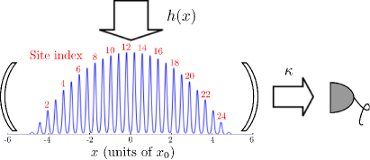
Figure 1: (Color online) The system of interest in Sec. VI. A condensate confined by the static external potential of Eq. (42) is placed inside an optical cavity with coupling function $g(x)=g_{0}\sin(kx)$. The initial condensate density is shown as the blue solid line, and since the optical lattice potential is commensurate with the cavity mode, peaks of density correspond to maxima of $|g(x)|$. The atoms are pumped transversely by the spatially constant $h(x)=h_{0}$, and photons lost through the cavity mirrors at a rate $\kappa$ are detected by a photon counter. Lattice sites are numbered from left to right, with the centermost sites being numbered $12$ and $13$.

We here numerically simulate a BEC of $N$ atoms, assuming that the system is confined in an elongated 1D trap, and we ignore any density fluctuations of the atoms along the radial direction. The system we consider is illustrated in Fig. 1. In the axial dimension, atoms are subject to a combined potential of a harmonic trap and a static optical lattice commensurate with the cavity mode

$$V(x)=\frac{1}{2}m\omega^{2}x^{2}+sE_{R}\cos^{2}(kx).$$ (42)

Atoms are therefore trapped at the antinodes of $g(x)$ and we choose a lattice height of $s=10$, where $E_{R}=\hbar^{2}k^{2}/2m$ is the recoil energy of a photon. The harmonic potential confines the system, and defines the dimensionless length $x_{0}=\sqrt{\hbar/m\omega}$, and time $t_{0}=1/\omega$ scales that we use to present the results in this and the following Section. As the initial state we consider atoms in the ground state of the combined trapping potential in the absence of any pump field, with $k\approx 8.1x_{0}^{-1}$, such that approximately $22$ sites of the lattice have significant population. For simplicity, we assume that the quantum and thermal fluctuations in the initial state are sufficiently small that they can be ignored. As a consequence, any difference in behavior for individual trajectories stems directly from the backaction of different measurement records. The system is pumped for times $t>0$ by a transverse beam $h(x)=h_{0}$, illuminating all sites equally. The remaining parameters defining the system are $NU\approx 38\hbar\omega x_{0}$, and $h_{0}^{2}g_{0}^{2}/\kappa\Delta_{pa}^{2}\approx 2.6\times 10^{-3}\omega$. We evolve the system for a number of independent measurement trajectories by numerically solving Eq. (40) using the Milstein algorithm Gardiner (2009). We analyze the results at the end of the simulations by decomposing the numerically calculated classical field $\psi(x)$ at different times into a lattice site basis Isella and Ruostekoski (2006); Cattani et al. (2013), also taking into account that the Wigner distribution returns symmetrically (instead of normally) ordered quantum-mechanical expectation values.

In this configuration, the measurement operator of Eq. (35) has a value $\langle\hat{Y}\rangle$ which is approximately proportional to the population imbalance $N_{\mathrm{odd}}-N_{\mathrm{even}}$, where $N_{\mathrm{odd(even)}}$ is the total population in the odd (even) sites of the lattice. Monitoring the intensity of light leaking from the cavity therefore approximately measures $(N_{\mathrm{odd}}-N_{\mathrm{even}})^{2}$. Consequently, from Eq. (41) we expect that the continuous quantum measurement process will lead to relative stochastic phase evolution of the atom field between different sites. Figure 2(a) shows the relative matter wave phase between the two central sites for two distinct measurement trajectories, each conditioned on a different measurement record. The fluctuations in relative phase differ between realizations, but in both cases an increase with time in the amplitude of the fluctuations in relative phase can be seen. Ensemble averaging over many realizations, Fig. 2(b) shows that the unconditioned dynamics leads to a phase decoherence between sites due to dissipation, with a rate depending upon the separation of the sites. Sites separated by an even number experience the same sign of $g(x)$ and so remain more phase coherent.

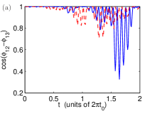
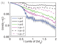
Figure 2: (Color online) Quantum measurement-induced phase evolution of the atomic field inside a cavity and the resulting phase decoherence in ensemble-averaged dynamics. (a) Relative phase variation between the atomic field in the two central lattice sites for two distinct measurement trajectories. (b) Ensemble averaged cosine of the phase between atoms in different lattice sites, averaged over 400 measurement realizations, showing dissipation induced decoherence. The phases are plotted between site $i=12$, and sites differing in number by i - j = 2,-2,-7,3,-1,1 (upper to lower curves,respectively). The shaded region for the $i-j=1$ curve represents one standard deviation of the sampling error in the results. A frequency analysis of the rapid oscillations evident in the curves reveals an interplay of several excited collective modes, supporting the need for a multimode treatment such as we present in this paper.

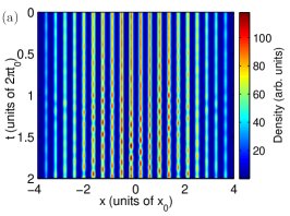
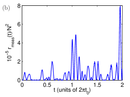
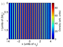
Figure 3: (Color online) Quantum measurement induced symmetry breaking in atomic density evolution, conditioned on a measurement record. (a) Time dependence of the stochastic field density $|\psi(x,t)|^{2}$ for a single measurement trajectory, conditioned on a single measurement record. This trajectory corresponds to the phase evolution shown in Fig. 2(a) [blue, solid line]. (b) The measurement rate of photons at the detector for the single trajectory shown in (a). Ensemble averaged time dependence of the stochastic field density $|\psi(x,t)|^{2}$, averaged over $400$ realizations, which restores the unbroken spatial pattern.

Since we start with a symmetric gas of atoms the initial expectation value of the light intensity inside the cavity vanishes due to destructive interference between the odd and even sites. For a single measurement trajectory, the stochastic phase fluctuations between odd and even sites due to photon detection lead to small population fluctuations between sites, and allow a nonvanishing intracavity light intensity. These population differences build and we see the atoms self-organize into an odd or even site pattern. The density variation for a single measurement trajectory is shown in Fig. 3(a). Self-organization initially becomes pronounced at the outer sites where the density is low, before propagating inwards to the high density region. The onset of self-organization throughout the system increases the value of $\langle\hat{Y}\rangle$, and therefore increases the measurement backaction. This is evident in the increase in phase fluctuations after about $0.5$ trap periods in Fig. 2(a). Ensemble averaging over many trajectories, the enhanced phase fluctuations after that time lead in turn to an enhanced rate of phase decoherence in the unconditioned results of Fig. 2(b).

Since neither pattern is energetically preferred, different measurement trajectories spontaneously break the symmetry into either pattern without favor. This example demonstrates the substantial effect a continuous quantum measurement process can impart on a BEC. We do not see the atoms stabilize into a constant pattern. In fact, we see the pattern oscillate between odd and even sites, similar to a Josephson like oscillation. The extent of self-organization and the oscillations between patterns show up in the rate of measured photons, Fig. 3(b), with peaks corresponding to significant population imbalance between odd and even sites.

Steady-state spontaneous self-organization has been much studied for thermal gases Domokos and Ritsch (2002); Asbóth et al. (2005); Ritsch et al. (2013) and BECs Nagy et al. (2008) in optical cavities, and experimentally observed, e.g., in 2D systems Black et al. (2003); Baumann et al. (2010). However, as Fig. 4 shows, our parameter regime is well below the pump power threshold for the onset of steady-state self-organization. The self-organization we observe here is therefore qualitatively different from the well-studied steady-state phenomenon, in that it exists only as a dynamical effect, resulting in oscillations between the two patterns.

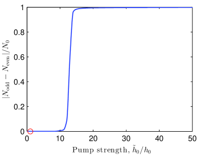
Figure 4: (Color online) Steady-state self-organization: Steady-state relative population imbalance due to self-organization as a function of pumping strength, $\tilde{h}_{0}$ in the units of $h_{0}$ – the pumping strength used for the classical measurement trajectories in this Section and highlighted by the red circle in the figure ($h_{0}^{2}g_{0}^{2}/\kappa\Delta_{pa}^{2}\approx 2.6\times 10^{-3}\omega$). We solve the steady-state problem using the classical Gross-Pitaevskii equation approach as detailed in Ref. Nagy et al. (2008), but calculated for our finite system in the harmonic potential trap. Self-organization is seen to occur for factors $\tilde{h}_{0}/h_{0}\gtrsim 10$.

We emphasize that the phase fluctuations and the self-organization in our model of the far-detuned transversely pumped atom-cavity case comes solely from the measurement backaction. The stochastic noise associated with the intensity measurement of light leaked from the cavity in each individual run of the classical trajectory conditions the dynamical evolution of the atoms inside the cavity and the subsequent measurement record. The measurements lead to the spontaneous breaking of the symmetry in the spatial density pattern of the atom cloud. If we ensemble-average over many independent stochastic realizations the broken symmetry in the atomic density is restored and we can recover the uniform density pattern, as illustrated in Fig. 3(c).

VI.2 Spatially nonuniform transverse pump

Owing to the multimode nature of the classical stochastic measurement trajectories, we can also investigate the backaction of a continuous quantum measurement process on spatially selective regions of the multimode atomic field. In the present case the measurement can be constructed to be spatially selective by employing a nonuniform profile for the driving field $h(x)$, and so directly cause phase noise in only a limited number of sites. For the same initial state as previously, we illuminate the system by a transverse beam with a Gaussian profile tailored to principally illuminate only a handful of sites in the lattice, illustrated in Fig. 5(a). In addition, to show only the dynamics due to the continuous measurement, we include an additional potential chosen to exactly compensate the light shift term in Eq. (40) arising from the spatially varying transverse beam.

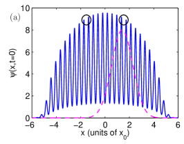
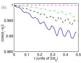
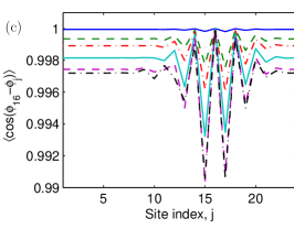
Figure 5: (Color online) Ensemble averaged phase decoherence of the atomic field inside a cavity, when the stochastic phase evolution for a single trajectory is proportional to the spatially varying strength of the quantum measurement backaction. We show Gaussian transverse pump results for a BEC in an optical lattice potential. (a) Initial state $\psi(x,t=0)$ (solid) and transverse pump beam profile $h(x)$ (red, dashed). The circles indicate the pair of sites most illuminated ($16,17$) and the corresponding pair on the other side of the condensate which is not illuminated ($8,9$). (b) Ensemble-averaged cosine of the relative phase between different sites. Lower to upper curves correspond to the following pairs of sites: pair of most illuminated sites ($16,17$) (blue, solid); sites ($16,13$) (black, dashed); sites ($16,12$) (green, dash-dotted); sites ($8,9$) (red, dashed). (c) Ensemble-averaged cosine of the phase relative to site $16$ for all other sites at different times, showing the spread of the phase decoherence with time. From upper to lower lines, the corresponding times are $(0.025,0.5,1.0,1.5,2.0,2.5)2\pi t_{0}$ respectively. Parameters as given for Sec. VI.1, and ensemble averaged over $200$ realizations.

Ensemble averaging over many realizations, the spread of the decoherence with time through the system can be seen in Fig. 5(b-c). The sites illuminated by the transverse beam accrue relative phase fluctuations due to the measurement, as seen in the constant illumination results. In contrast, atoms in sites which are not measured remain in phase at short times. At longer times, the tunneling between lattice sites then allows the phase evolution to propagate through to sites which are not illuminated, and a more complicated many-body dynamics is set up. Averaging over many independent trajectories exhibiting these phase fluctuations results in spatially varying phase decoherence corresponding to the dynamics of the unconditioned master equation (36) due to dissipation from the open system, as illustrated in Fig. 5(b-c).

VII Quantum measurement in an optomechanical multimode system

Due to the position sensitivity of the coupling of cavity light to the atoms, the dynamics of the cavity mode can couple to the mechanical motion of the BEC, a realization of an optomechanical system. When the atom cloud occupies a larger spatial region or the amplitude of the mechanical oscillations is not small, a simple linear optomechanical treatment is no longer valid. Incorporating the backaction of a continuous quantum measurement process, when the light leaking out of the cavity is monitored, provides an additional challenge.

In this Section we show how a continuous monitoring of the intensity of the cavity output generates multimode optomechanical dynamics of a condensate in a cavity. The intrinsic multimode excitations of the BEC are solely the consequence of the conditioned measurement record of a single stochastic realization, and ensemble-averaging over a large number of realizations cancels out any overall optomechanical motion in the atomic density. Using classical measurement trajectories, we will show that the measurement can be tailored to preferentially excite selected intrinsic excitations. The optomechanical condensate dynamics with interacting collective mode excitations cannot be adequately represented by a single- or few-mode model; furthermore, inclusion of a sufficient number of modes is infeasible for quantum trajectory simulations.

Cavity optomechanics  Kippenberg and Vahala (2007, 2008); Meystre (2013); Aspelmeyer et al. (2013) provides a useful tool to study the interface between quantum and classical regimes, coupling a quantized light field to a meso- or macroscopic mechanical system, such as a mirror that is free to oscillate or a gas of atoms within the cavity. The sensitivity of such systems to the position of the oscillator has several potential applications in quantum sensing Braginsky et al. (1980); Caves et al. (1980), and the coupling with the light can be used to control the mechanical system, for example cooling of the macroscopic motional state Horak et al. (1997); Vuletić and Chu (2000). Nanomechanical resonators have now been cooled to the quantum regime O’Connell et al. (2010); Teufel et al. (2011); Chan et al. (2011). In contrast, ultracold atomic gases can routinely be cooled to the quantum degenerate regime, and the technical challenges of cooling optomechanical systems that are commonplace for most mechanical oscillators can be circumvented. For ultracold gases in a cavity, we have an optomechanical system where a quantized light field is coupled to a many-body multimode optomechanical system that is already in its ground state, allowing a variety of optomechanical responses Zhang et al. (2009); Chen et al. (2010); Larson and Martikainen (2010); Brahms and Stamper-Kurn (2010); De Chiara et al. (2011).

In the following Section we briefly review the more commonly discussed linear optomechanical regime, before returning to focus on the multimode problem in the subsequent Section.

VII.1 Linear optomechanical regime

Current experiments on cavity optomechanics with ultracold atoms have generally operated in the linear optomechanical regime, where the cavity light strongly couples only with a single excitation mode of the atoms. Such a regime can be reached by having a cavity wavelength much smaller than the extent of the atom cloud, such that it predominantly Bragg diffracts the atoms between the states with momentum $0$ and $\pm\hbar k$ Brennecke et al. (2008). The linear regime is reached provided that higher momentum states play a negligible role. Alternatively, atoms can be tightly trapped via a strong external optical lattice. Provided that each atom cloud can move only a small amplitude from the lattice site minimum, the linear regime is again reached with the dominant dynamics being due to a single collective mode Murch et al. (2008); Schleier-Smith et al. (2011). In this regime, the system is well described by the coupled Hamiltonian for the cavity light mode and the single motional mode $\hat{b}$

$$H_{\mathrm{lin}}=\hbar\omega_{b}\hat{b}^{\dagger}\hat{b}+\hbar\omega^{\prime}_{c}\hat{a}^{\dagger}\hat{a}+\hbar g^{\prime}(\hat{b}+\hat{b}^{\dagger})\hat{a}^{\dagger}\hat{a}\,,$$ (43)

where $\omega^{\prime}_{c}$ includes the shift to the cavity resonance frequency from the atoms, and $g^{\prime}$ is a generalized coupling strength between the atomic mode and the cavity photons. We can recover this form of Hamiltonian from our Eq. (6) by, for example, assuming a tightly confined condensate with a spatial extent smaller than the cavity wavelength, pumped on the cavity axis. This could also represent a single site of an optical lattice where the atoms occupy more than one site with negligible tunneling between the sites, provided the system can be approximated as translationally invariant. Under the approximations that the condensate center-of-mass undergoes small displacements of $\delta x$, centered at $x_{0}$, but without exciting any other perturbations in the shape of the condensate density, then the spatial integral in the coupling term of Eq. (6) becomes

$$\frac{\hbar}{\Delta_{pa}}\int\hat{\Psi}^{\dagger}(x)g^{2}(x)\hat{\Psi}(x)\mathrm{d}x\hat{a}^{\dagger}\hat{a}\approx\frac{\hbar}{\Delta_{pa}}g_{0}^{2}\sin(kx_{0})\delta x\hat{a}^{\dagger}\hat{a}.$$ (44)

Quantization of the center-of-mass motion, such that $\delta x=(\hat{b}+\hat{b}^{\dagger})/\sqrt{2}$ then leads to the linear optomechanical Hamiltonian. Similar Hamiltonians can be derived in the transversely pumped case, but the essential approximation is that the integral $\int g^{2}(x)|\psi(x)|^{2}\mathrm{d}x\propto\delta x$ ($\int h(x)g(x)|\psi(x)|^{2}\mathrm{d}x\propto\delta x$ for the transversely pumped case). These are the same integrals which appear in the measurement operators $\langle\hat{X}\rangle$ and $\langle\hat{Y}\rangle$ of Eqs. (26) and (35), and hence photon detection implies a backaction on the atoms which couples to the single mode $\hat{b}$ in this regime.

VII.2 Multimode optomechanical system

In contrast to the linear optomechanical regime, we study here the case where the measurement can cause density perturbations of the condensate which are not insignificant, center-of-mass displacement which is not restricted to be small, and where the interactions between atoms in the condensate can couple together different quasiparticle excitations. The single-mode model commonly used to describe the condensate in the linear optomechanical regime is therefore insufficient to describe this many-mode problem and the richer physics we expect to result. Our classical treatment of the continuous quantum measurement process is particularly suitable for such a problem. The computational efficiency of the classical trajectories allows us to simulate a condensate on a spatial grid with upwards of $1024$ points, a problem whose full quantum trajectory calculation is not numerically feasible.

VII.2.1 The system

In this Section we are interested in the atom dynamics in a single potential well, and therefore simulate a BEC confined within an optical cavity by the harmonic external potential

$$V(x)=\frac{1}{2}m\omega^{2}x^{2},$$ (45)

where we will assume the wavelength of the cavity to be of the same order as the radius of the BEC. This system also represents the translationally invariant case of many BECs in a periodic potential with negligible tunneling, with each BEC coupled identically.

The atoms are pumped transversely with a uniform driving field $h(x)=h_{0}$ on resonance with the cavity mode frequency, and we study the dynamics in the limit of an adiabatically eliminated cavity field presented in Sec. V.2. In this limit, we emphasize that the sole dynamical contribution from the cavity mode is due to measurement backaction. Since we will begin in an eigenstate of the atomic Hamiltonian, all dynamics studied in this Section are therefore purely measurement induced. Detection of the light leaking out of the cavity represents a combined measurement of many of the collective excitation modes of the atoms–these describe the intrinsic dynamical degrees of freedom for a BEC in a multimode picture. The quantum measurement can lead to complex dynamics by exciting several of the interacting modes. Nonetheless, we show that a suitable tailoring of the cavity mode shape can be used to selectively excite particular collective modes of the atom cloud.

We calculate the classical measurement trajectories using Eq. (40), which has two free parameters. We set the interaction nonlinearity $NU\approx 64\hbar\omega x_{0}$, and the ratio $h_{0}^{2}g_{0}^{2}/\kappa\Delta_{pa}^{2}\approx 0.042\omega$. In order to make the role of measurement backaction more transparent, we operate in the weakly fluctuating limit where the quantum and thermal fluctuations in the initial state are assumed to be negligible. In this limit the only difference between trajectories comes from the distinct backaction of the continuous quantum measurement process; the dynamics of the system generated by Eq. (40) for different trajectories arise directly from a given measurement record for an individual experimental run. The quantum fluctuations of the initial state may be ignored provided the depletion of the BEC is small, which for our nonlinearity requires $N\gg 14$ at zero temperature. More strongly fluctuating cases could be studied using the approaches discussed in Sec. VIII.

All quantities can be rescaled for an atom number $N$, given the fixed nonlinearity, and the measurement rate then scales as $r_{\mathrm{meas}}(t)\propto N^{2}$. However, in addition to the classical limit above, the atom number must satisfy two constraints. Firstly, the measurement rate must be sufficiently high if we expect to resolve the dynamics of the atoms inside the cavity–this requires a significant number of measurement events during the characteristic time of the excitation to be observed. Secondly, the small parameter in our adiabatic expansion $\int(g^{2}(x)/\Delta_{pa})|\psi(x)|^{2}\mathrm{d}x/\kappa$ must remain much less than unity. As an example, choosing $\kappa=100\omega$, $g_{0}/\sqrt{\Delta_{pa}}=0.16\omega^{1/2}$ and $h_{0}/\sqrt{\Delta_{pa}}=12.8\omega^{1/2}$, we find an atom number in the range $500-1000$ adequately satisfies these various constraints for the dominant excitations that we study below.

VII.2.2 Decomposition into Bogoliubov-de-Gennes modes

We simulate the effect of continuous quantum measurement on the optomechanical motion of a BEC inside the cavity. Starting from the ground state of the BEC, we begin to transversely pump the atoms on resonance with the cavity at $t=0$ with an aim to excite collective motion of the condensate via the measurement process. Collective motion of the condensate can be decomposed, for weak excitations, into the intrinsic excitation modes of the system – the linearized Bogoliubov-de-Gennes (BdG) quasiparticle modes. A semiclassical treatment of cavity cooling for the unconditioned case using such a decomposition was presented in Gardiner et al. (2001). The quasiparticle modes $u_{i}(x)$ and $v_{i}(x)$ are the solutions to the BdG equations

$$\begin{array}[]{lcr}{\cal L}(x)u_{i}(x)-NU\psi_{0}^{2}(x)v_{i}(x)&=&\varepsilon_{i}u_{i}(x),\\ {\cal L}(x)v_{i}(x)-NU[\psi_{0}^{*}(x)]^{2}u_{i}(x)&=&-\varepsilon_{i}v_{i}(x),\end{array}$$ (46)

in the subspace orthogonal to the stationary initial state of the condensate $\psi_{0}(x)$, where

$${\cal L}(x)=H_{0}-\mu+2NU|\psi_{0}(x)|^{2}.\\$$ (47)

We can now define quasiparticle mode amplitudes $\alpha_{i}$ Morgan et al. (1998), such that

$$\psi(x,t) =e^{-i\mu t/\hbar}\bigg{\{}\alpha_{0}(t)\psi_{0}(x)$$

$$+\sum_{i\neq 0}\left[\alpha_{i}(t)u_{i}(x)-\alpha_{i}^{*}(t)v_{i}^{*}(x)\right]\bigg{\}},$$ (48)

where $|\alpha_{0}|^{2}$ is the number of particles in the state $\psi_{0}(x)$ which is normalized to $\int\mathrm{d}x|\psi_{0}(x)|^{2}=1$. Projecting the results of our classical measurement trajectory onto the BdG modes then gives the time dependent mode amplitudes

$$\alpha_{i}=\int\mbox{d}x\left[u^{*}_{i}(x)\psi(x)e^{i\mu t/\hbar}+v_{i}^{*}(x)\psi^{*}(x)e^{-i\mu t/\hbar}\right].$$ (49)

We can now use the BdG mode decomposition to express the measurement operator $\hat{Y}$ from Eq. (35). Detection of a photon lost from the cavity represents a combined measurement of many of the collective modes of the condensate, dictated by the functional form of $\hat{Y}$, and corresponds to the jump operator of Eq. (38). When the stochastic field $\psi(x,t)$ is close to the initial configuration – assuming that $\alpha_{0}$ is macroscopically occupied, but the remaining excitation modes have low population – then $\langle\hat{Y}\rangle$ is approximately

$$\langle\hat{Y}\rangle= \frac{h_{0}}{\Delta_{pa}}\bigg{\{}|\alpha_{0}|^{2}\int g(x)|\psi_{0}(x)|^{2}\mathrm{d}x$$

$$+\sum_{i\neq 0}\alpha_{0}^{*}\int g(x)\psi^{*}_{0}(x)\left[\alpha_{i}u_{i}(x)-\alpha_{i}^{*}v_{i}(x)\right]\mathrm{d}x\bigg{\}}.$$ (50)

We can therefore attempt to couple the measurement backaction to a chosen mode by maximizing the corresponding overlap integral

$$O_{i}=\int g(x)\psi_{0}^{*}(x)\left[u_{i}(x)-v_{i}(x)\right]\mathrm{d}x.$$ (51)

VII.2.3 Center-of-mass excitation

As a first example, we study how the continuous measurement can induce an optomechanical coupling of the center-of-mass mode, and for a BEC in a harmonic potential this corresponds to exciting the lowest energy BdG collective mode, the Kohn mode. We choose the wavelength of the cavity mode such that the overlap integral for the Kohn mode, $O_{1}$, from Eq. (51) is maximized. Figure 6(a) shows the form of the resulting cavity coupling function $g(x)$, along with the initial state of the atoms, and the Kohn mode quasiparticle functions $u_{1}(x)$ and $v_{1}(x)$.

For this geometry, Fig. 6(b)-(f) demonstrate the measurement backaction for two distinct realizations of single measurement trajectories. As anticipated, the condensate acquires a pronounced center-of-mass oscillation. The oscillations are revealed as pulses in the measured rate of photocounts, since the overlap of the stochastic field $\psi(x,t)$ with the cavity mode $g(x)$ varies with time and consequently affects the number of photons pumped into the cavity mode. For notational simplicity, we use the variable $q$ to represent moments of $x$ for individual realizations, i.e. $q_{1}=\int x|\psi(x)|^{2}\mathrm{d}x$, $q_{2}=\int x^{2}|\psi(x)|^{2}\mathrm{d}x$, and use the brackets $\langle\rangle$ to represent quantum averages, obtained by ensemble averaging normal ordered operators over many single trajectories Gardiner and Zoller (2004); Martin and Ruostekoski (2010).

Due to the stochastic nature of the continuous measurement process, different realizations corresponding to distinct measurement records display different trajectories for the evolution of the atomic density. BdG mode amplitudes and phases also vary between realizations. This measurement-induced symmetry breaking of the dynamics of the atoms is similar to that seen in the density patterns of Sec. VI. The initial unbroken symmetry in the atomic density is restored on ensemble averaging over a large number of independent trajectories, so as to generate the dynamics from the unconditioned master equation (36). Figure 7 shows that the unconditioned dynamics lead to no overall motion of the condensate density, instead the condensate stochastic field decoheres due to dissipation induced by the open nature of the system.

Nonetheless, ensemble averaging quantities extracted from single trajectories, such as the populations of BdG modes and center-of-mass coordinates as presented in Fig. 8, illuminate the average response of single realizations. As intended, the BdG mode decomposition shows that the predominant excitation at short times is the Kohn mode. However, several other low energy modes also respond to the measurement, confirming that we are not in the linear optomechanical regime with only a single mechanical mode. Most notably, the second BdG mode becomes dominant at later times, this is the breathing mode which corresponds to a collective excitation of $\Delta q=\sqrt{q_{2}-q_{1}^{2}}$. Since the breathing mode has a different parity with respect to the trap center than the cavity mode $g(x)$ we would not naively expect it to respond to the measurement backaction. At early times, the breathing mode occupation is indeed small, but once the center-of-mass oscillations move the condensate off center, the breathing mode can become excited. Of course, the BdG mode decomposition is only valid while the condensate is not significantly perturbed from the initial state, and so should not be relied upon at later times. However, confirmation of the qualitative behavior indicated by the BdG modes is given by Fig. 8(b) showing that the average center-of-mass displacement continues to grow slowly at large times, and Fig. 6(f) showing that $\Delta q$ does begin to oscillate at the time that the breathing mode population becomes significant.

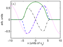
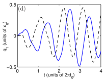
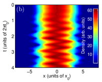
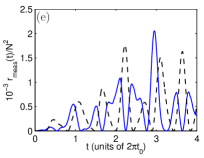
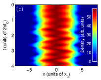
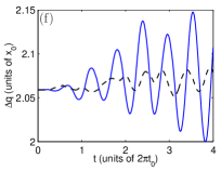
Figure 6: (Color online) A selective excitation of collective modes of a BEC as a result of quantum measurement backaction. (a) Comparison of the shapes of the Kohn mode quasiparticle functions $u_{1}(x)$ (blue, dashed) and $v_{1}(x)$ (black, dash-dotted) with the cavity mode function $g(x)$ (red, dotted), and the initial stochastic field for the condensate $\psi(x)$ (green, solid), for the case where the overlap of the cavity mode and the Kohn mode is maximal. The differing quantities have been scaled into arbitrary units to enable a comparison of their functional form. (b)-(f) The dynamics for a single stochastic realization of a measurement record when maximizing the overlap of the cavity mode with the Kohn mode. (b) & (c) The stochastic field density $|\psi(x,t)|^{2}$ as a function of time for two different classical measurement trajectories. The transverse pump beam is applied at $t=0$ and remains at a constant strength throughout the simulation. (d) The center-of-mass position of the condensate for the two trajectories shown in (b) (solid) and (c) (dashed). (e) The measurement rate of photons at the photo-detector $r_{\mathrm{meas}}$ for the two trajectories, directly proportional to the measured photocurrent. (f) The variation of $\Delta q$ for the two trajectories.

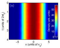
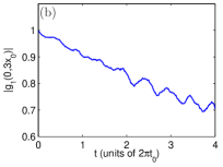
Figure 7: (Color online) Condensate response to the transverse pump unconditioned on any particular measurement trajectory, formed by ensemble averaging $400$ single trajectories such as are shown in Fig. 6. (a) Ensemble averaged stochastic field density $|\psi(x,t)|^{2}$. (b) Dissipation induced loss of coherence between $x=0$ and $x^{\prime}=3x_{0}$. The figure shows $|g_{1}(x,x^{\prime})|\equiv|\langle\hat{\Psi}^{\dagger}(x)\hat{\Psi}(x^{\prime})\rangle|$, the initial condensate is phase coherent with $|g_{1}(x,x^{\prime})|=1$.

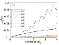
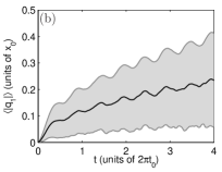
Figure 8: (Color online) Quantum measurement-induced excitation of the Kohn mode, simulations with a maximum overlap between $g(x)$ and the Kohn mode. (a) Decomposition into BdG linearized collective excitations, mode occupation numbers are shown averaged over $400$ individual measurement trajectories. (b) Ensemble average of $\langle|q_{1}|\rangle$ over $400$ realizations, note the absolute value must be taken since the measurement backaction generates oscillations with a random phase for different realizations.

Even though other modes are excited, at short times the Kohn mode is the dominant excitation. To verify the above argument that the overlap between the Kohn mode and the cavity mode function governs the degree of excitation, Fig. 9 shows the Kohn mode excitation and the center-of-mass displacement after a short time as a function of the cavity mode wavelength. The response agrees well with the behavior of the overlap integral (51). Away from the peak overlap the Kohn mode response reduces substantially, becoming particularly weak at $k=1.03x_{0}^{-1}$. This point closely corresponds to the peak overlap of the third BdG mode, which Fig. 10 shows is strongly excited. In contrast to the Kohn mode results, this mode remains the dominant excitation throughout the length of our simulation.

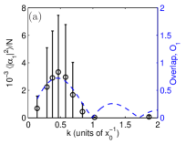
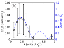
Figure 9: (Color online) Varying the wavelength of the light in the cavity compared to the Kohn mode wavelength. (a) The Kohn mode population, and (b) the center-of-mass displacement $\langle|q_{1}|\rangle$, after a short time ($0.162\pi t_{0}$) as a function of the cavity mode wavelength. Error bars represent the quantum mechanical uncertainty. The results have been ensemble averaged over $400$ realizations for each cavity wavelength.

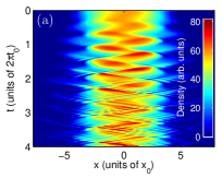
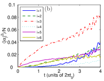
Figure 10: (Color online) Response for a cavity wavelength of $k=1.03x_{0}^{-1}$, corresponding to the point second from the right in Fig. 9. (a) Density response stochastic field $|\psi(x,t)|^{2}$ for a single stochastic realization of a measurement record. (b) BdG mode populations, ensemble averaged over $400$ realizations.

VII.2.4 Breathing mode excitation

Moving the trap center to a cavity antinode means that the measurement can be tailored to couple to a mode of different parity. Tuning the cavity wavelength to maximize the overlap with the breathing mode leads to the results in Fig. 11. The response to the measurement backaction differs significantly from the previous results, as is clearly seen by the stochastic field density $|\psi(x)|^{2}$. The center-of-mass displacement is negligible at all times, while both the the BdG mode decomposition and the behavior of $\langle\Delta q\rangle$ show the breathing mode to be strongly excited. The oscillations set up by the breathing mode are easily identifiable in the observed measurement rate. Note that in contrast to the previous results, here the initial state is not orthogonal to $g(x)$, and so the initial measurement rate is significantly greater. Once again, a number of low energy collective modes are substantially occupied. However, in contrast to the Kohn mode results, since the breathing mode excitation preserves the parity of the stochastic field $\psi(x)$, all the modes populated have the same parity as the breathing mode, even at long times.

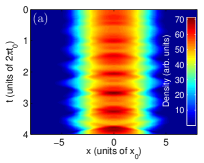
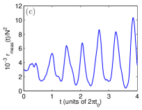
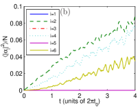
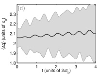
Figure 11: (Color online) Quantum measurement-induced excitation of the breathing mode. Maximal breathing mode overlap results: (a) Density of the stochastic field $|\psi(x,t)|^{2}$ as a function of time for a single stochastic realization of a measurement record. (b) Ensemble average over $400$ realizations of BdG mode populations. (c) Measurement rate for the same single realization as that shown in (a). (d) Ensemble average of $\Delta q=\sqrt{q_{2}-q_{1}^{2}}$. The shaded gray area corresponds to the width of the standard deviation in the result.

VIII Initial configurations with enhanced fluctuations

We may also consider situations where the initially stable equilibrium configuration exhibits notable quantum or thermal fluctuations. In order to model more accurately the resulting dynamics of the atom-light cavity system, we may apply many-body theories for the calculation of the initial phase-space quasi-probability distribution. Stochastic sampling of the initial states for the time evolution of SDEs can then synthesize the quantum-statistical correlations of the initial state. For simplicity, we consider the initial configuration of the atoms in the ground state inside the cavity in the absence of the light. The simplest approach that includes the spatial variation of the density and phase fluctuations of the atoms Isella and Ruostekoski (2006) is to sample the initial noise according to the Bogoliubov theory. We expand the initial state for the stochastic representation of the bosonic field operator in terms of the Bogoliubov modes $u_{j}(x)$ and $v_{j}(x)$ as

$${\psi}(x)=\psi_{0}(x)\alpha_{0}+\sum_{j\neq 0}[u_{j}(x)\alpha_{j}-v_{j}^{*}(x)\alpha_{j}^{*}]\,.$$ (52)

where $\psi_{0}(x)$ denotes the ground-state solution and the total number of ground state atoms $N_{c}=\langle\hat{\alpha}_{0}^{\dagger}\hat{\alpha}_{0}\rangle$. The stochastic mode amplitudes $\alpha_{j}$ and $\alpha_{j}^{*}$ are sampled from the corresponding Wigner distribution for harmonic oscillators Gardiner and Zoller (2004) in order to synthesize the fluctuations of an ideal Bose-Einstein distribution for the phonons $\langle\hat{\alpha}_{j}^{\dagger}\hat{\alpha}_{j}\rangle=[\exp{(\varepsilon_{j}/k_{B}T)}-1]^{-1}$. The normal mode frequencies $\varepsilon_{j}$ and the quasi-particle amplitudes $u_{j}$ and $v_{j}$ in the initial trapping potential can be solved numerically. In a more strongly fluctuating case the quasi-particle modes and the ground-state condensate profile may be solved self-consistently using the Hartree-Fock-Bogoliubov theory Gross et al. (2011); Cattani et al. (2013). A strongly confined 1D system may also exhibit enhanced phase fluctuations that can be incorporated using a quasi-condensate representation Martin and Ruostekoski (2010).

IX Concluding remarks

The backaction of measurement on a quantum system is an intrinsic feature of quantum mechanics. However, when the system has a large number of particles and modes, it is not computationally feasible to obtain a numerical solution to the nonlinear dynamics that incorporates the backaction of the continuous quantum measurement process within a full quantum picture. Here we have presented an unraveling of the classical quasi-probability amplitude for a many mode system, namely a BEC in an optical cavity, into classical measurement trajectories which approximate a continuous quantum measurement process, conditioned on a given measurement record.

We have derived a Fokker-Planck equation for the evolution of the ensemble averaged quasi-probability distribution given by the Wigner function, in the limit of weak quantum fluctuations. The Fokker-Planck equation is then mapped onto SDEs, where the dynamical noise in each stochastic realization is generated by the measurement record on a photon detector. Each stochastic trajectory is therefore conditioned on a particular probabilistic measurement record that represents a classical approximation of the backaction of a continuous quantum measurement process. Each stochastic measurement trajectory corresponds to the measurement record of a potential individual experimental run. Since a continuously measured observable in few- or many-body systems is expected to be closely approximated by classical dynamics whenever the measurements are frequent enough to be able to resolve the dynamics Javanainen and Ruostekoski (2013), the method can predict the dynamics of the observed quantity even deep in the quantum regime.

We have then numerically studied the continuous measurement of a large multimode atomic BEC consisting of up to 1024 spatial grid points inside an optical cavity. The intensity of light leaking out of the cavity is continuously monitored and this has a direct effect on the cavity photon amplitude, which in turn couples to the atoms inside the cavity. In the limit that the cavity field may be adiabatically eliminated, the measurement of the light intensity outside the cavity can be directly related to the spatial profile of the atomic field. We find that the atoms inside the cavity undergo local stochastic phase evolution that solely results from the backaction of the measurement process. The phase noise is proportional to the spatially varying strength of the quantum measurement. We have shown how this local phase evolution can lead to quantum measurement-induced pattern formation for a BEC. The continuous quantum measurement process spontaneously breaks the symmetry of the spatial profile of the multimode BEC. The pattern emerges randomly, conditioned on the detection record of the photons. Ensemble-averaging over many stochastic measurement trajectories restores the initial uniform unbroken spatial condensate density profile, and demonstrates the loss of coherence between sites due to dissipation from the open system.

In the absence of an additional optical lattice, we have studied the effects of a continuous quantum measurement on the optomechanical motion of a BEC inside the cavity. In a multimode representation a BEC exhibits a large number of intrinsic dynamical degrees of freedom in terms of its collective excitations that couple to the cavity mode. We have shown how the measurement can be tailored to selectively excite particular collective modes of a BEC–considering examples of Kohn and breathing modes. The interaction between the modes lead to spreading of the excitations between different modes and eventually a more complex internal dynamics.

We have limited ourselves in this paper to approximate classical theories that are severely restricted by the computational demands of large realistic multimode systems. It would be particularly interesting to explore how classical approximations make dynamical trajectories more objective than their fully quantum-mechanical counterparts and whether our classical measurement trajectories are affected by the choice of measurement scheme, such as photon counting, homodyne or heterodyne measurements Carmichael (1993); Wiseman and Milburn (1993). The backaction of homodyne measurements has been studied for simplified models of BECs in cavities Corney and Milburn (1998), in dispersive imaging Dalvit et al. (2002); Szigeti et al. (2009), and in an interferometric context Lee et al. (2012) (related to the experiments of Ref. Saba et al. (2005)); the photon counting of scattered light was simulated in Refs. Ruostekoski and Walls (1998, 1997). Experimentally, the backaction of a continuous quantum measurement process has been confirmed for BECs in heterodyne measurements of the cavity output Murch et al. (2008); Brahms et al. (2012). In addition, the results of the measurement can be used to construct feedback mechanisms Wiseman and Milburn (2010). For condensates feedback has been studied in the context of reducing heating due to measurement backaction Hush et al. (2013).

Appendix A Adiabatic elimination of light mode

As a more rigorous adiabatic elimination of the light mode, we outline here a derivations which follows closely in spirit a procedure explained in greater detail in Carmichael (2007). Without the presence of atoms, the cavity mode would be well represented by a coherent state of amplitude $\alpha_{0}=\eta/(\kappa-i\Delta_{pc})$, we therefore use a displacement operator ${\cal D}[\alpha_{0}]$ to shift away this contribution, by defining the displaced density matrix

$$\rho_{D}={\cal D}[\alpha_{0}]\rho{\cal D}^{\dagger}[\alpha_{0}].$$ (53)

Performing this transformation on the master equation, we can conveniently write the result

$$\dot{\rho_{D}}=({\cal S}_{d}+{\cal S}_{a}+{\cal S}_{da})\rho_{D},$$ (54)

in terms of the superoperators

$${\cal S}_{d}\rho= i\Delta_{pc}\left[\hat{a}^{\dagger}\hat{a},\rho\right]+\kappa\left(2\hat{a}\rho\hat{a}^{\dagger}-\rho\hat{a}^{\dagger}\hat{a}-\hat{a}^{\dagger}\hat{a}\rho\right),$$ (55)

$${\cal S}_{a}\rho= -\frac{i}{\hbar}\left[H_{4},\rho\right],$$ (56)

$${\cal S}_{da}\rho= -i\int\mathrm{d}x\frac{g^{2}(x)}{\Delta_{pa}}\Bigg{\{}\left[\hat{\Psi}^{\dagger}(x)\hat{a}^{\dagger}\hat{a}\hat{\Psi}(x),\rho\right]$$

$$+\left[\hat{\Psi}^{\dagger}(x)\left(\frac{\eta}{\kappa-i\Delta_{pc}}\hat{a}^{\dagger}+\frac{\eta^{*}}{\kappa+i\Delta_{pc}}\hat{a}\right)\hat{\Psi}(x),\rho\right]\Bigg{\}}.$$ (57)

These define, respectively, the evolution of the the atomic and displaced cavity mode subsystems, and that due to the interaction, and we have defined

$$H_{4}= \int\mbox{d}x\hat{\Psi}^{\dagger}(x)\left\{-\frac{\hbar^{2}}{2m}\nabla^{2}+V(x)\right\}\hat{\Psi}(x)$$

$$+\frac{U}{2}\int\mbox{d}x\hat{\Psi}^{\dagger}(x)\hat{\Psi}^{\dagger}(x)\hat{\Psi}(x)\hat{\Psi}(x)$$

$$+\hbar\frac{|\eta|^{2}}{\kappa^{2}+\Delta_{pc}^{2}}\int\mbox{d}x\frac{g^{2}(x)}{\Delta_{pa}}\hat{\Psi}^{\dagger}(x)\hat{\Psi}(x).$$ (58)

We have therefore shifted the dominant coherent contribution from the interaction of the atoms with the cavity mode into an effective potential in the atomic operator subspace Hamiltonian. With the further transformation

$$\bar{\rho}_{D}=e^{-({\cal S}_{d}+{\cal S}_{a})t}\rho_{D},$$ (59)

the master equation simplifies to

$$\dot{\bar{\rho}}_{D}(t)=\bar{{\cal S}}_{da}(t)\bar{\rho}_{D}(t),$$ (60)

where

$$\bar{{\cal S}}_{da}(t)=e^{-({\cal S}_{d}+{\cal S}_{a})t}{\cal S}_{da}e^{({\cal S}_{d}+{\cal S}_{a})t}.$$ (61)

Formal integration of Eq. (60) leads to

$$\bar{\rho}_{D}(t)=\bar{\rho}_{D}(0)+\int_{0}^{t}\bar{{\cal S}}_{da}(t^{\prime})\bar{\rho}_{D}(t^{\prime})\mathrm{d}t^{\prime}.$$ (62)

We may now eliminate our displaced cavity mode, which we assume to be well approximated by the vacuum state since the predominant contribution to the cavity mode was shifted away by our earlier displacement. We therefore substitute on the RHS of Eq. (62)

$$\rho_{D}(t)\approx\rho_{a}(t)\otimes(|0\rangle_{d}\mbox{}_{d}\langle 0|),$$ (63)

where $|0\rangle_{d}$ is the vacuum state vector for the displaced cavity field. Upon tracing over the displaced cavity field, the first term of Eq. (62) can be seen to vanish. The remaining term, after some superoperator algebra Carmichael (2007), and reversal of the transformation of Eq. (59), gives the adiabatically eliminated master equation for the atomic field only

$$\dot{\rho}_{a}(t)= -\frac{i}{\hbar}\left[H_{4},\rho_{a}(t)\right]-i\Delta_{pc}\frac{|\eta|^{2}}{(\kappa^{2}+\Delta_{pc}^{2})^{2}}\left[\hat{X}\hat{X},\rho_{a}(t)\right]$$

$$+\kappa\frac{|\eta|^{2}}{(\kappa^{2}+\Delta_{pc}^{2})^{2}}\left(2\hat{X}\rho_{a}(t)\hat{X}-\hat{X}\hat{X}\rho_{a}(t)-\rho_{a}(t)\hat{X}\hat{X}\right).$$ (64)

If we assume that $\Delta_{pc}\ll\kappa$, and expand in the small parameters $\hat{X}/\kappa,\Delta_{pc}/\kappa$, then we obtain the same result at lowest order as the simpler treatment given in Sec. V.1, leading to the classical measurement trajectories given by Eq. (32). The advantage of the method presented in this Appendix is the ability to consistently go beyond the lowest order. The next highest order contribution is due to the second term of Eq. (64), and gives rise to the second term of Eq. (33).

References

- Joos and Zeh (1985) E. Joos and H. D. Zeh, Z. Phys. B 59, 223 (1985).
- Zurek (2003) W. H. Zurek, Rev. Mod. Phys. 75, 715 (2003).
- Walls and Milburn (1985) D. F. Walls and G. J. Milburn, Phys. Rev. A 31, 2403 (1985).
- Leggett and Sols (1991) A. J. Leggett and F. Sols, Found. Phys. 21, 353 (1991).
- Drummond and Corney (1999) P. D. Drummond and J. F. Corney, Phys. Rev. A 60, R2661 (1999).
- Gardiner et al. (1998) C. W. Gardiner, M. D. Lee, R. J. Ballagh, M. J. Davis, and P. Zoller, Phys. Rev. Lett. 81, 5266 (1998).
- Poletti et al. (2012) D. Poletti, J.-S. Bernier, A. Georges, and C. Kollath, Phys. Rev. Lett. 109, 045302 (2012).
- Ruostekoski and Walls (1998) J. Ruostekoski and D. F. Walls, Phys. Rev. A 58, R50 (1998).
- Weiler et al. (2008) C. N. Weiler, T. W. Neely, D. R. Scherer, A. S. Bradley, M. J. Davis, and B. P. Anderson, Nature 455, 948 (2008).
- Khodorkovsky et al. (2009) Y. Khodorkovsky, G. Kurizki, and A. Vardi, Phys. Rev. A 80, 023609 (2009).
- Witthaut et al. (2009) D. Witthaut, F. Trimborn, and S. Wimberger, Phys. Rev. A 79, 033621 (2009).
- Olmos et al. (2013) B. Olmos, D. Yu, Y. Singh, F. Schreck, K. Bongs, and I. Lesanovsky, Phys. Rev. Lett. 110, 143602 (2013).
- Pichler et al. (2010) H. Pichler, A. J. Daley, and P. Zoller, Phys. Rev. A 82, 063605 (2010).
- Cockburn et al. (2010) S. P. Cockburn, H. E. Nistazakis, T. P. Horikis, P. G. Kevrekidis, N. P. Proukakis, and D. J. Frantzeskakis, Phys. Rev. Lett. 104, 174101 (2010).
- Witthaut et al. (2011) D. Witthaut, F. Trimborn, H. Hennig, G. Kordas, T. Geisel, and S. Wimberger, Phys. Rev. A 83, 063608 (2011).
- Gilz and Anglin (2011) L. Gilz and J. R. Anglin, Phys. Rev. Lett. 107, 090601 (2011).
- Höning et al. (2013) M. Höning, D. Muth, D. Petrosyan, and M. Fleischhauer, Phys. Rev. A 87, 023401 (2013).
- Syassen et al. (2008) N. Syassen, D. M. Bauer, M. Lettner, T. Volz, D. Dietze, J. J. García-Ripoll, J. I. Cirac, G. Rempe, and S. Dürr, Science 320, 1329 (2008).
- Diehl et al. (2008) S. Diehl, A. Micheli, A. Kantian, B. Kraus, H. P. Büchler, and P. Zoller, Nat. Phys. 4, 878 (2008).
- Jenkins and Ruostekoski (2012) S. D. Jenkins and J. Ruostekoski, Phys. Rev. A 86, 031602 (2012).
- Leroux et al. (2010) I. D. Leroux, M. H. Schleier-Smith, and V. Vuletić, Phys. Rev. Lett. 104, 073602 (2010).
- Chen et al. (2011) Z. Chen, J. G. Bohnet, S. R. Sankar, J. Dai, and J. K. Thompson, Phys. Rev. Lett. 106, 133601 (2011).
- Wiseman and Milburn (2010) H. Wiseman and G. Milburn, Quantum Measurement and Control (Cambridge University Press, 2010).
- Tian and Carmichael (1992) L. Tian and H. J. Carmichael, Phys. Rev. A 46, R6801 (1992).
- Dalibard et al. (1992) J. Dalibard, Y. Castin, and K. Mølmer, Phys. Rev. Lett. 68, 580 (1992).
- Dum et al. (1992) R. Dum, P. Zoller, and H. Ritsch, Phys. Rev. A 45, 4879 (1992).
- Carmichael (1993) H. Carmichael, An Open Systems Approach to Quantum Optics (Springer, Berlin, 1993).
- Javanainen and Ruostekoski (2013) J. Javanainen and J. Ruostekoski, New J. Phys. 15, 013005 (2013).
- Javanainen and Yoo (1996) J. Javanainen and S. M. Yoo, Phys. Rev. Lett. 76, 161 (1996).
- Cirac et al. (1996) J. I. Cirac, C. W. Gardiner, M. Naraschewski, and P. Zoller, Phys. Rev. A 54, R3714 (1996).
- Castin and Dalibard (1997) Y. Castin and J. Dalibard, Phys. Rev. A 55, 4330 (1997).
- Ruostekoski and Walls (1997) J. Ruostekoski and D. F. Walls, Phys. Rev. A 56, 2996 (1997).
- Carmichael (2007) H. Carmichael, Statistical Methods in Quantum Optics (Springer, Berlin, 2007), Vol. 2.
- Brennecke et al. (2007) F. Brennecke, T. Donner, S. Ritter, T. Bourdel, M. Kohl, and T. Esslinger, Nature 450, 268 (2007).
- Murch et al. (2008) K. W. Murch, K. L. Moore, S. Gupta, and D. M. Stamper-Kurn, Nat. Phys. 4, 561 (2008).
- Brahms et al. (2012) N. Brahms, T. Botter, S. Schreppler, D. W. C. Brooks, and D. M. Stamper-Kurn, Phys. Rev. Lett. 108, 133601 (2012).
- Brennecke et al. (2008) F. Brennecke, S. Ritter, T. Donner, and T. Esslinger, Science 322, 235 (2008).
- Botter et al. (2013) T. Botter, D. W. C. Brooks, S. Schreppler, N. Brahms, and D. M. Stamper-Kurn, Phys. Rev. Lett. 110, 153001 (2013).
- Ritsch et al. (2013) H. Ritsch, P. Domokos, F. Brennecke, and T. Esslinger, Rev. Mod. Phys. 85, 553 (2013).
- Horak and Ritsch (2001) P. Horak and H. Ritsch, Phys. Rev. A 63, 023603 (2001).
- Gardiner et al. (2001) S. A. Gardiner, K. M. Gheri, and P. Zoller, Phys. Rev. A 63, 051603 (2001).
- Nagy et al. (2008) D. Nagy, G. Szirmai, and P. Domokos, Eur. Phys. J. D 48, 127 (2008).
- Szirmai et al. (2009) G. Szirmai, D. Nagy, and P. Domokos, Phys. Rev. Lett. 102, 080401 (2009).
- Kónya et al. (2011) G. Kónya, G. Szirmai, and P. Domokos, Eur. Phys. J. D 65, 33 (2011).
- Moore et al. (1999) M. G. Moore, O. Zobay, and P. Meystre, Phys. Rev. A 60, 1491 (1999).
- Niedenzu et al. (2013) W. Niedenzu, S. Schütz, H. Habibian, G. Morigi, and H. Ritsch, Phys. Rev. A 88, 033830 (2013).
- Mekhov and Ritsch (2009) I. B. Mekhov and H. Ritsch, Phys. Rev. Lett. 102, 020403 (2009).
- Hush et al. (2013) M. R. Hush, S. S. Szigeti, A. R. R. Carvalho, and J. J. Hope, New J. Phys. 15, 113060 (2013).
- Szigeti et al. (2009) S. S. Szigeti, M. R. Hush, A. R. R. Carvalho, and J. J. Hope, Phys. Rev. A 80, 013614 (2009).
- Jaynes and Cummings (1963) E. Jaynes and F. W. Cummings, Proc. IEEE 51, 89 (1963).
- Walls and Milburn (1994) D. F. Walls and G. J. Milburn, Quantum Optics, 2nd ed. (Springer, Berlin, 1994).
- Maschler et al. (2008) C. Maschler, I. B. Mekhov, and H. Ritsch, Eur. Phys. J. D 46, 545 (2008).
- Gardiner and Zoller (2004) C. Gardiner and P. Zoller, Quantum Noise (Springer, Berlin, 2004).
- Steel et al. (1998) M. J. Steel, M. K. Olsen, L. I. Plimak, P. D. Drummond, S. M. Tan, M. J. Collett, D. F. Walls, and R. Graham, Phys. Rev. A 58, 4824 (1998).
- Sinatra et al. (2002) A. Sinatra, C. Lobo, and Y. Castin, J. Phys. B 35, 3599 (2002).
- Isella and Ruostekoski (2006) L. Isella and J. Ruostekoski, Phys. Rev. A 74, 063625 (2006).
- Blakie et al. (2008) P. B. Blakie, A. S. Bradley, M. J. Davis, R. J. Ballagh, and C. W. Gardiner, Adv. Phys. 57, 363 (2008).
- Martin and Ruostekoski (2010) A. D. Martin and J. Ruostekoski, Phys. Rev. Lett. 104, 194102 (2010).
- Polkovnikov (2010) A. Polkovnikov, Ann. Phys. (N.Y.) 325, 1790 (2010).
- Opanchuk and Drummond (2013) B. Opanchuk and P. D. Drummond, J. Math. Phys. 54, 042107 (2013).
- Norrie et al. (2006a) A. A. Norrie, R. J. Ballagh, C. W. Gardiner, and A. S. Bradley, Phys. Rev. A 73, 043618 (2006a).
- Ruostekoski and Isella (2005) J. Ruostekoski and L. Isella, Phys. Rev. Lett. 95, 110403 (2005).
- Norrie et al. (2006b) A. A. Norrie, R. J. Ballagh, and C. W. Gardiner, Phys. Rev. A 73, 043617 (2006b).
- Carmichael (2010) H. Carmichael, Statistical Methods in Quantum Optics (Springer, Berlin, 2010), Vol. 1.
- Gross et al. (2011) C. Gross, J. Estève, M. K. Oberthaler, A. D. Martin, and J. Ruostekoski, Phys. Rev. A 84, 011609 (2011).
- Cattani et al. (2013) F. Cattani, C. Gross, M. K. Oberthaler, and J. Ruostekoski, New J. Phys. 15, 063035 (2013).
- (67) P. W. Anderson, in The Lesson of Quantum Theory edited by J. de Boer, E. Dal, and O. Ulfbeck (North-Holland, Amsterdam, 1986).
- Gardiner (2009) C. Gardiner, Stochastic Methods (Springer, Berlin, 2009), 4th ed.
- Domokos and Ritsch (2002) P. Domokos and H. Ritsch, Phys. Rev. Lett. 89, 253003 (2002).
- Asbóth et al. (2005) J. K. Asbóth, P. Domokos, H. Ritsch, and A. Vukics, Phys. Rev. A 72, 053417 (2005).
- Black et al. (2003) A. T. Black, H. W. Chan, and V. Vuletić, Phys. Rev. Lett. 91, 203001 (2003).
- Baumann et al. (2010) K. Baumann, C. Guerlin, F. Brennecke, and T. Esslinger, Nature 464, 1301 (2010).
- Kippenberg and Vahala (2007) T. J. Kippenberg and K. J. Vahala, Opt. Express 15, 17172 (2007).
- Kippenberg and Vahala (2008) T. J. Kippenberg and K. J. Vahala, Science 321, 1172 (2008).
- Meystre (2013) P. Meystre, Ann. Phys. (Leipzig) 525, 215 (2013).
- Aspelmeyer et al. (2013) M. Aspelmeyer, T. J. Kippenberg, and F. Marquardt, arXiv:1303.0733 (2013).
- Braginsky et al. (1980) V. B. Braginsky, Y. I. Vorontsov, and K. S. Thorne, Science 209, 547 (1980) .
- Caves et al. (1980) C. M. Caves, K. S. Thorne, R. W. P. Drever, V. D. Sandberg, and M. Zimmermann, Rev. Mod. Phys. 52, 341 (1980).
- Horak et al. (1997) P. Horak, G. Hechenblaikner, K. M. Gheri, H. Stecher, and H. Ritsch, Phys. Rev. Lett. 79, 4974 (1997).
- Vuletić and Chu (2000) V. Vuletić and S. Chu, Phys. Rev. Lett. 84, 3787 (2000).
- O’Connell et al. (2010) A. D. O’Connell, M. Hofheinz, M. Ansmann, R. C. Bialczak, M. Lenander, E. Lucero, M. Neeley, D. Sank, H. Wang, M. Weides, J. Wenner, J. M. Martinis, and A. N. Cleland, Nature 464, 697 (2010).
- Teufel et al. (2011) J. D. Teufel, T. Donner, D. Li, J. W. Harlow, M. S. Allman, K. Cicak, A. J. Sirois, J. D. Whittaker, K. W. Lehnert, and R. W. Simmonds, Nature 475, 359 (2011).
- Chan et al. (2011) J. Chan, T. P. M. Alegre, A. H. Safavi-Naeini, J. T. Hill, A. Krause, S. Gröblacher, M. Aspelmeyer, and O. Painter, Nature 478, 89 (2011).
- Zhang et al. (2009) J. M. Zhang, F. C. Cui, D. L. Zhou, and W. M. Liu, Phys. Rev. A 79, 033401 (2009).
- Chen et al. (2010) W. Chen, D. S. Goldbaum, M. Bhattacharya, and P. Meystre, Phys. Rev. A 81, 053833 (2010).
- Larson and Martikainen (2010) J. Larson and J.-P. Martikainen, Phys. Rev. A 82, 033606 (2010).
- Brahms and Stamper-Kurn (2010) N. Brahms and D. M. Stamper-Kurn, Phys. Rev. A 82, 041804 (2010).
- De Chiara et al. (2011) G. De Chiara, M. Paternostro, and G. M. Palma, Phys. Rev. A 83, 052324 (2011).
- Schleier-Smith et al. (2011) M. H. Schleier-Smith, I. D. Leroux, H. Zhang, M. A. Van Camp, and V. Vuletić, Phys. Rev. Lett. 107, 143005 (2011).
- Morgan et al. (1998) S. A. Morgan, S. Choi, K. Burnett, and M. Edwards, Phys. Rev. A 57, 3818 (1998).
- Wiseman and Milburn (1993) H. M. Wiseman and G. J. Milburn, Phys. Rev. A 47, 642 (1993).
- Corney and Milburn (1998) J. F. Corney and G. J. Milburn, Phys. Rev. A 58, 2399 (1998).
- Dalvit et al. (2002) D. A. R. Dalvit, J. Dziarmaga, and R. Onofrio, Phys. Rev. A 65, 053604 (2002).
- Lee et al. (2012) M. D. Lee, S. Rist, and J. Ruostekoski, New J. Phys. 14, 073057 (2012).
- Saba et al. (2005) M. Saba, T. A. Pasquini, C. Sanner, Y. Shin, W. Ketterle, and D. E. Pritchard, Science 307, 1945 (2005).