The Grow-Shrink strategy for learning Markov network structures constrained by context-specific independences

Abstract

Markov networks are models for compactly representing complex probability distributions. They are composed by a structure and a set of numerical weights. The structure qualitatively describes independences in the distribution, which can be exploited to factorize the distribution into a set of compact functions. A key application for learning structures from data is to automatically discover knowledge. In practice, structure learning algorithms focused on “knowledge discovery” present a limitation: they use a coarse-grained representation of the structure. As a result, this representation cannot describe context-specific independences. Very recently, an algorithm called CSPC was designed to overcome this limitation, but it has a high computational complexity. This work tries to mitigate this downside presenting CSGS, an algorithm that uses the Grow-Shrink strategy for reducing unnecessary computations. On an empirical evaluation, the structures learned by CSGS achieve competitive accuracies and lower computational complexity with respect to those obtained by CSPC.

1 Introduction

Markov networks are parametric models for compactly representing complex probability distributions of a wide variety of domains. These models are composed by two elements: a structure and a set of numerical weights. The structure plays an important role, because it describes a set of independences that holds in the domain, thus making assumptions about the functional form or factorization of the distribution [5]. For this reason, the structure is an important source of knowledge discovery because it depicts intricate patterns of probabilistic (in)dependences between the domain variables. Usually, the structure of a Markov network can be constructed by algorithms using observations taken from an unknown distribution. Interestingly, the constructed structure can be used by human experts for discovering unknown knowledge [16]. For this reason, the problem of structure learning from data has received an increasing attention in machine learning [14, 9, 8]. However, Markov network structure learning from data is still challenging. One of the most important problems is that it requires weight learning that cannot be solved in closed-form, requiring to perform a convex optimization with inference as a subroutine. Unfortunately, inference in Markov networks is #P-complete [8].

As a result, structure learning algorithms seek the “best” approximation to the solution structure, making assumptions about the form of the solution space or the used objective function. The choice of these approximations depends on the goal of learning used for designing learning algorithms [8, Chapter 16]. In generative learning, we can find two goals of learning: density estimation, where a structure is “best” when the resulting Markov network is accurate for answering inference queries; and knowledge discovery, where a structure is “best” when it is accurate for qualitatively describing the independences that hold in the distribution. Depending on the goal of learning, we can categorize structure learning algorithms in: density estimation algorithms [4, 11]; and knowledge discovery algorithms [1, 15]. In this work, we are focusing in the knowledge discovery goal.

In practice, knowledge discovery algorithms exploit the fact that the structure can be viewed as a set of independences. Thus, for constructing a structure, such algorithms successively make (in)dependence queries to data in order to restrict the number of possible structures, converging toward the solution structure. To achieve a good performance in this procedure, knowledge discovery algorithms use a sound and complete representation of the structure: a single undirected graph. A graph can be viewed as an inference engine which efficiently represents and manipulates (in)dependences in polynomial time [14]. Unfortunately, this graph representation cannot capture a type of independences known as context-specific independences [6, 7, 8]. For these cases, knowledge discovery algorithms cannot achieve good results in their goal of learning, because a single graph cannot capture such independences, obscuring the acquisition of knowledge. To overcome this limitation, a novel knowledge discovery algorithm has recently been developed [3]. This algorithm, called CSPC, uses an alternative representation of the structure called canonical models, a particular class of Context Specific Interaction models (CSI models) [7]. Canonical models allow us to encode context-specific independences by using a set of mutually independent graphs. Using this representation, CSPC can learn more accurate structures than several state-of-the-art algorithms. However, despite the benefits in accuracy, CSPC presents an important downside: it has a high computational complexity, because it must perform a large number of independence queries in comparison to traditional algorithms.

Therefore, this paper focuses on reducing the number of independence queries required for learning canonical models. This reduction was thought in order to achieve competitive accuracies with respect to CSPC, but avoiding unnecessary queries. To achieve this, we present the CSGS algorithm, a knowledge discovery algorithm that learns canonical models by using the Grow-Shrink strategy [12] in a similar way to the GSMN algorithm, a Markov network structure learning algorithm [1]. Basically, under the assumption of bounded maximum degree, this strategy constructs a structure in polynomial time by identifying local neighborhoods of each variable [12]. On an empirical evaluation, the canonical models learned by CSGS achieve competitive accuracies and lower time complexity with respect to those obtained by CSPC.

The remaining of this work is structured as follows: Section 2 reviews essential concepts. Section 3 presents our contribution: CSGS. Next, Section 4 shows our empirical evaluation of CSGS on synthetic datasets. Finally, Section 5 concludes with directions for future work.

2 Background

We introduce our general notation. Hereon, we use the symbol $V$ to denote a finite set of indexes. Lowercase subscripts denote particular indexes, for instance $a,b\in V$; in contrast, uppercase subscripts denote subsets of indexes, for instance $W\subseteq V$. Let $X_{V}$ be a set of random variables of a domain, where single variables are denoted by single indexes in $V$, for instance $X_{a},X_{b}\in X_{V}$ where $a,b\in V$. We simply use $X$ instead of $X_{V}$ when $V$ is clear from the context. We focus on the case where $X$ takes discrete values $x\in\operatorname{Val}(V)$, that is, the values for any $X_{a}\in X$ are discrete: $\operatorname{Val}(a)=\{x_{a}^{0},x_{a}^{1},\ldots\}$. For instance, for boolean-valued variables, that is $|\operatorname{Val}(a)|=2$, the symbols $x^{0}_{a}$ and $x^{1}_{a}$ denote the assignments $X_{a}=0$ and $X_{a}=1$, respectively. Moreover, we overload the symbol $V$ to also denote the set of nodes of a graph. Finally, we use $\mathcal{X}\subseteq\operatorname{Val}(V)$ for denoting an arbitrary set of complete or canonical assignments, that is, all the variables take a fixed value. For instance, $x_{V}^{i}\equiv x^{i}\in\operatorname{Val}(V)$.

2.1 Conditional and context-specific independences

A set of independence assumptions is commonly called the structure of a distribution because independences determine the factorization, or functional form, of a distribution. Two of the most known types of independences are conditional and context-specific independences. The latter has received an increased interest [6, 7, 8, 2, 3], because one conditional independence can be expressed as a set of context-specific independences. Formally, context-specific independences are defined as follows:

Definition 1

Let $A,B,U,W\subseteq V$ be disjoint subsets of indexes, and let $x_{W}$ be some assignment in $\operatorname{Val}(W)$. Let $p(X)$ be a probability distribution. We say that variables $X_{A}$ and $X_{B}$ are contextually independent given $X_{U}$ and the context $X_{W}=x_{W}$, denoted by $I({X_{A}},{X_{B}}\mid X_{U},x_{W})$, iff $p(X)$ satisfies:

$$p(x_{A}|x_{B},x_{U},x_{W})=p(x_{A}|x_{U},x_{W}),$$

for all assignments $x_{A}$, $x_{B}$, and $x_{U}$; whenever $p(x_{B},x_{U},x_{W})>0$.

As a consequence, if $I({X_{A}},{X_{B}}\mid X_{U},x_{W})$ holds in $p(X)$, then it logically follows that $I({x_{A}},{x_{B}}\mid x_{U},x_{W})$ also holds in $p(X)$ for any assignment $x_{A}$, $x_{B}$, $x_{U}$. Interestingly, if $I({X_{A}},{X_{B}}\mid X_{U},x_{W})$ holds for all $x_{W}\in\operatorname{Val}(W)$, then we say that the variables are conditionally independent. Formally,

Definition 2

Let $A,B,U,W\subseteq V$ be disjoint subsets of indexes, and let $p(X)$ be a probability distribution. We say that variables $X_{A}$ and $X_{B}$ are conditionally independent given $X_{U}$ and $X_{W}$, denoted by $I({X_{a}},{X_{b}}\mid X_{U},X_{W})$, iff $p(X)$ satisfies:

$$p(x_{A}|x_{B},x_{U},x_{W})=p(x_{A}|x_{U},x_{W}),$$

for all assignments $x_{A}$, $x_{B}$, $x_{U}$, and $x_{W}$; whenever $p(x_{B},x_{U},x_{W})>0$.

Thus, a conditional independence $I({X_{A}},{X_{B}}\mid X_{U},X_{W})$ that holds in $p(X)$ can be seen as a conjunction of context-specific independences of the form $\bigwedge_{x_{W}}I({X_{A}},{X_{B}}\mid X_{U},x_{W})$ for all $x_{W}\in\operatorname{Val}(W)$. Moreover, each context-specific independence $I({X_{A}},{X_{B}}\mid X_{U},x_{W})$, that holds in $p(X)$, can be seen as a conditional independence $I({X_{A}},{X_{B}}\mid X_{U})$ that holds in the conditional distribution $p(X_{V\setminus W}|x_{W})$[2].

2.2 Representation of structures

The independence relation $I({\cdot},{\cdot}\mid\cdot)$ commonly assumes the Markov properties [9, Section 3.1]; we also assume that probability distributions are positive. Thus, an isomorphic mathematical object that conforms to the previous properties is an undirected graph [14]. An undirected graph $G$ is a pair $(V,E)$, where $E\subset V\times V$ is a set of edges which encodes conditional independences by using the graph-theoretic notion of reachability. As a result, the independence assertion $I({X_{A}},{X_{B}}\mid X_{U})$ can be associated with the graphical condition: “every path from A to B is intercepted by the nodes U”. Therefore, a graph $G$ encodes knowledge in a readily accessible way, that is, the graph is highly interpretable. For instance, we can determine the adjacencies of a node $a\in V$, or its Markov blanket $\operatorname{MB}({a~{}\colon~{}G})\subseteq V\setminus\{a\}$, from its neighboring nodes in the graph $G$. Unfortunately, the use of a single graph as representation presents an issue when distributions hold context-specific independences, because it only encodes conditional independences, leading to excessively dense graphs [2, 3].

In practice, for overcoming the previous limitation, an alternative representation of the structure consists in a set $\mathcal{F}=\{f^{i}_{D}\}$ of features, where each feature is commonly represented as an indicator function (Kronecker’s delta), that is, a boolean-valued function $f_{D}:\operatorname{Val}(D)\mapsto\{0,1\}$. Given an arbitrary assignment $x$, a feature $f^{i}_{D}(x)$ returns 1, if $x_{D}=x^{i}_{D}$; and $0$ otherwise. A set of features is a more flexible representation than a graph, because the former can encode context-specific independences. For example, an independence of the form $I({X_{a}},{X_{b}}\mid x_{W})$ is encoded in $\mathcal{F}$ iff for any feature $f^{i}_{D}\in\mathcal{F}^{\prime}=\{f^{i}_{D}~{}\in~{}\mathcal{F}~{}\colon~{}x_{W}=x^{i}_{W}~{}\wedge~{}W\subseteq D\}$, the variables $X_{a}$ and $X_{b}$ do not appear simultaneously in the set $D$, that is, either $a\notin D$ or $b\notin D$. From a set $\mathcal{F}$ of features, we can induce a graph $G$ by adding an edge between every pair of nodes whose variables appear together in some feature $f^{i}_{D}\in\mathcal{F}$ [3]. In a similar way, following our previous example, we can induce a graph from $\mathcal{F}^{\prime}\subseteq\mathcal{F}$. This graph is known as an instantiated graph $G(x^{i}_{W})=(V,E,x^{i}_{W})$, namely, a graph $G=(V,E)$ whose nodes $W\subseteq V$ are associated to the assignment $x^{i}_{W}\in\operatorname{Val}(W)$ [6]. Unfortunately, a set of features is not easily interpretable as a single graph, because we cannot efficiently verify independence assertions, since we are required to check all the features in $\mathcal{F}$.

A graph representation for overcoming the previous limitations is canonical models [3]. These models are a proper subset of the CSI models [6, 7], which can capture context-specific independences in a more interpretable way than a set of features. A canonical model $\bar{}\mathcal{G}$ is a pair $(\mathcal{G},\mathcal{X})$, where $\mathcal{G}$ is a collection of instantiated graphs of the form $\mathcal{G}=\{G(x^{i})\in\mathcal{G}~{}:~{}x^{i}\in\mathcal{X}\subseteq\operatorname{Val}(V)\}$, and $\mathcal{X}$ is a set of canonical assignments. These instantiated graphs are called canonical graphs, because every graph $G(x^{i})$ is associated to a canonical assignment $x^{i}\in\operatorname{Val}(V)$. In contrast to a single graph $G$, a canonical model requires several canonical graphs for capturing both conditional and context-specific independences. For instance, let us suppose that we want to encode the context-specific independence $I({X_{a}},{X_{b}}\mid x_{w})$ in a canonical model $\bar{}\mathcal{G}$. By Definition 2.1, this independence implies a set of independences of the form $I({x_{a}},{x_{b}}\mid x_{w})$, for all the assignments $x_{a},x_{b}\in\operatorname{Val}(a),\operatorname{Val}(b)$. Then, each independence $I({x_{a}},{x_{b}}\mid x_{w})$ is captured by a particular $G(x^{i})\in\mathcal{G}$, one whose context $x^{i}$ satisfies: $x_{a}^{i}=x_{a}$, $x_{b}^{i}=x_{b}$, and $x_{w}^{i}=x_{w}$.

2.3 Markov networks

A Markov network is a parametric model for representing probability distributions in a compact way. This model is defined by a structure and a set of potential functions $\{\phi_{k}(X_{D_{k}})\}_{k}$, where $\phi_{k}:\operatorname{Val}(D_{k})\mapsto\mathbb{R}^{+}$, and $X_{D_{k}}\subseteq X$ is known as the scope of $\phi_{k}$. For discrete domains, a usual representation of the potential functions is a table-based function. Markov networks can represent a very important class of probability distributions called Gibbs distributions, whose functional form is as follows: $p(X=x)=\frac{1}{Z}\prod_{k}\phi_{k}(x_{D_{k}})$, where $Z$ is a global constant, called partition function, that guarantees the normalization of the product. A Gibbs distribution $p(X)$ factorizes over a graph $G$, if any scope $X_{D_{k}}$ corresponds to a complete subgraph $D_{k}$ (a.k.a. clique) of the graph $G$. Without loss of generality, the Gibbs distribution is often factorized by using the maximum cliques of the graph $G$. For positive distributions, one important theoretical result states the converse [5], that is, $p(X)$ can be represented as a Gibbs distribution (Markov network) that factorizes over $G$, if $G$ is an I-map for $p(X)$. As a result, given a positive Gibbs distribution $p(X)$, it can be shown that every influence on any variable $X_{a}\in X$ can be blocked by conditioning on its Markov blanket $\operatorname{MB}({a~{}\colon~{}G})$, formally: $p(X_{a}|X_{V\setminus\{a\}})=p(X_{a}|X_{\operatorname{MB}({a})})$. Interestingly, an extension of the previous property provides a criterion for determining the presence or absence of any edge $(a,b)$ in an I-map graph $G$ as follows [15, Theorem 1]:

Proposition 1

Let $p(X)$ be a positive Gibbs distribution. Then, for any $a\in V$:

1. the set of assertions $\{I({X_{a}},{X_{b}}\mid X_{\operatorname{MB}({a})\setminus\{b\}})~{}\colon~{}b\in\operatorname{MB}({a})\}$ is false in $p(X)$, presence of an edge $(a,b)$, iff each assertion satisfies $p(X_{a},X_{b}|X_{\operatorname{MB}({a})})\neq p(X_{a}|X_{\operatorname{MB}({a})})\cdot p(X_{b}|X_{\operatorname{MB}({a})})$.

2. the set of assertions $\{I({X_{a}},{X_{b}}\mid X_{\operatorname{MB}({a})})~{}\colon~{}b\notin\operatorname{MB}({a})\}$ is true in $p(X)$, absence of an edge $(a,b)$, iff each assertion satisfies $p(X_{a},X_{b}|X_{\operatorname{MB}({a})})=p(X_{a}|X_{\operatorname{MB}({a})})\cdot p(X_{b}|X_{\operatorname{MB}({a})})$.

Although a Gibbs distribution makes the structure explicit, it encodes the potential functions as a table-based function, obscuring finer-grained structures such as context-specific independences [8]. For this reason, a commonly used representation of a Markov network is the log-linear model defined as $p(x)=\frac{1}{Z}\exp\left\{~{}\sum_{k}\sum_{i}w_{i,k}f^{i}_{k}(x_{D_{k}})\right\}.$ A log-linear model can be constructed from a Gibbs distribution as follows: for the $i$th row of the table-based potential function $\phi_{k}$, an indicator function $f^{i}_{k}(\cdot)$ is defined whose weight is $w_{i,k}=\log\phi_{k}(x^{i}_{D_{k}})$.

3 Context-Specific Grow-Shrink algorithm

In this section we present CSGS (Context-Specific Grow-Shrink), a knowledge discovery algorithm for learning the structure of Markov networks by using canonical models as structure representation. The design of CSGS was inspired by the search strategy used by CSPC for learning canonical models [3], and the GS search strategy for learning graphs [12, 1]. Therefore, CSGS obtains a canonical model by learning a collection $\mathcal{G}$ of mutually independent canonical graphs, where each canonical graph $G(x^{i})\in\mathcal{G}$ is learned by using the GS strategy. More precisely, GS obtains a graph in two steps: first, it generalizes an initial very specific graph (one that makes many independence assumptions) by adding edges. Then, the resulting graph is specialized by removing spurious edges. In sum, Algorithm 1 shows an overview of CSGS. In line 1 and 1, CSGS defines an initial specific canonical model from a set of canonical assignments $\mathcal{X}$. Subsequently, lines 1 and 1 construct each canonical graph $G(x^{i})\in\mathcal{G}$ by using the GS strategy. For determining the presence or absence of an edge, CSGS uses Proposition 1 as criterion. The validation of this criterion is realized by eliciting context-specific independences from data in a similar way to CSPC [3, Section 4.3]. Finally, in a similar fashion to CSPC [3, Section 4.4], CSGS uses the resulting canonical model $\bar{}\mathcal{G}$ for generating a set $\mathcal{F}$ of features in order to enable us to use standard software packages for performing weight learning and inference. The remaining of this section is structured by using the key elements of CSGS: i) Section 3.1 describes how the initial canonical model is defined; ii) Section 3.2 presents the GS strategy for obtaining the canonical graphs; and iii) Section 3.3 concludes analyzing the time complexity of CSGS.

Input: domain $V$, dataset $\mathcal{D}$

1

2$\mathcal{X}\leftarrow$ Define the set of canonical assignments

3$\mathcal{G}\leftarrow$ Define a set of initial graphs $\{G(x^{i})\colon x^{i}\in\mathcal{X}\}$

4foreach $G(x^{i})\in\mathcal{G}$ do

5       $G(x^{i})\leftarrow$ GS($G(x^{i})$, $\mathcal{D}$)

6$\mathcal{F}\leftarrow$ Feature generation from $\bar{}\mathcal{G}=(\mathcal{G},\mathcal{X})$

Algorithm 1 Overview of CSGS

3.1 Initial canonical model

The definition of the initial canonical model consists, firstly, in the set of canonical assignments $\mathcal{X}$. In a similar fashion to CSPC [3], this set is composed by the unique training examples in $\mathcal{D}$. This definition is the consequence of using the data-driven approach, that is, we use only contexts that appear in data, and for the remaining contexts which do not appear in the data, we assume that they are improbable due to the lack of other information. Lastly, once $\mathcal{X}$ is defined, we associate the most specific graph $G(x^{i})$ to each context $x^{i}\in\mathcal{X}$, namely, the empty graph. As a result, in each initial canonical graph, every Markov blanket is empty. The idea behind the GS strategy is to add edges, thus adding nodes to each blanket.

3.2 Grow-Shrink strategy for learning canonical graphs

CSGS uses the GS strategy under the local-to-global approach [15, 11]. In this approach, the structure is obtained by constructing each Markov blanket $\operatorname{MB}({a}),a\in V$ in turn. In this manner, for each node $a$, the strategy GS determines the Markov blanket $\operatorname{MB}({a})$ in two phases: the grow phase and the shrink phase. The grow phase adds a new edge $(a,b)$ to $E$ as long as Proposition 1.1 is satisfied in data. However, due to the node ordering used [12, 1], the grow phase can add nodes that are outside of the blanket, resulting in spurious edges. For this reason, the shrink phase removes an edge $(a,b)\in E$ as long as Proposition 1.2 is satisfied in data. Algorithm 2 shows a more detailed description of the construction of the canonical graph $G(x^{i})$. Initially, the canonical graph $G(x^{i})$ is empty, then it is generalized by using the local-to-global approach shown in the loop of line 2. In this loop, the two steps of GS are performed: the grow phase, starting in line 2; and the shrink phase, starting in line 2. In each iteration of the main loop, line 2 and 2 change the Markov blanket by adding/removing new edges to the current set $E$ of edges. Once the main loop has finished, the Markov blankets of each node are obtained and, in consequence, the resulting canonical graph encodes context-specific independences.

Input: graph $G(x^{i})=(V,E,x^{i})$, dataset $\mathcal{D}$

1

2foreach node $a\in V$ do

3      

4      foreach node $b\in V\setminus({\operatorname{MB}({a~{}\colon~{}G(x^{i})})}\cup\{a\})$  do

5            

6            if $I({X_{a}},{X_{b}}\mid x^{i}_{\operatorname{MB}({a~{}\colon~{}G(x^{i})})})$ is false in $\mathcal{D}$ then

7                  

8                  $E\leftarrow E\cup(a,b)$

9      foreach $b\in\operatorname{MB}({a})$  do

10            

11            if $I({X_{a}},{X_{b}}\mid x^{i}_{\operatorname{MB}({a~{}\colon~{}G(x^{i})})\setminus\{b\}})$ is true in $\mathcal{D}$ then

12                  

13                  $E\leftarrow E\setminus(a,b)$

14return $G(x^{i})$

Algorithm 2 GS strategy

3.3 Asymptotic complexity

As is usual in knowledge discovery algorithms, we analyze the complexity of CSGS by determining the number of independence tests performed for constructing a structure from data. Let $m$ be the number of unique examples in the dataset, the complexity of performing a test is linear in $m$. However, this cost can be particularly high if $m$ is large. In our implementation of CSGS, we reduce this cost by using ADTree [13]. We assume that nodes in line 2 in Algorithm 2 are taken in an unspecified but fixed order, and we bound the maximum degree of a node to $k=\operatorname*{\arg\!\max}_{G(x^{i})\in\mathcal{G}}\operatorname*{\arg\!\max}_{a\in V}(|\operatorname{MB}({a~{}\colon~{}G(x^{i})})|)$. Let $n$ be the number of variables, and let $G(x^{i})=(V,E,x^{i})$ be an empty canonical graph, we can decompose the analysis into the number of tests performed by grow and shrink phases. In the grow phase, a test is performed for each edge $(a,b)\notin E$, resulting in $\operatorname{O}\bigl{(}n^{2}\bigr{)}$ tests. At the end of the grow phase, the size of a blanket is $k$ at worst, thus shrink phase performs $\operatorname{O}\bigl{(}nk\bigr{)}$ tests. Additionally, Algorithm 1 performs the GS strategy $m$ times, one per each initial canonical graph. Therefore, the total complexity is $\operatorname{O}\bigl{(}m(n^{2}+nk)\bigr{)}$ independence tests.

4 Empirical evaluation

This section shows experimental results obtained from the structures learned by CSGS and several structure learning algorithms on synthetic datasets. Basically, the goals of our experiments remark the greatly practical utility of our algorithm in a two-fold manner. First, we compare the accuracy of the structures learned by CSGS and CSPC, as well as by other state-of-the-art structure learners. Second, we compare the computational complexity between CSGS and CSPC. For evaluating the accuracy of the learned structures, we use the underlying distributions that were sampled to generate the synthetic datasets; since there is a direct correlation between the correctness of the structure and the accuracy of the distribution[5], the accuracy of a structure can be measured by comparing the similarity between the learned and underlying distributions. On the other hand, for evaluating the computational complexity, we report the number of tests performed for constructing the structures. Lastly, an open source implementation of CSGS algorithm as well as the synthetic datasets used in this section are publicly available.

4.1 Datasets

The datasets of our experiment are used in [2, 3] and were sampled from Markov networks with context-specific independences for different $n$ numbers of variables that range from 6 to 9, varying their sizes from 20 to 100k datapoints. For each $n$, 10 datasets were sampled from 10 different Markov networks with fixed structure but randomly choosing their weights. For more details, we refer the readers to [3, Appendix B]. Roughly speaking, the underlying structure of these models encodes independence assertions of the form $I({X_{a}},{X_{b}}\mid x^{1}_{w})$ for all pairs $a,b\in V\setminus\{w\}$, becoming dependent when $X_{w}=x^{0}_{w}$. In this way, the underlying structure can be seen as two instantiated graphs: a fully connected graph $G(x^{0}_{w})$, and a star graph $G(x^{1}_{w})$ whose central node is $x^{1}_{w}$. Despite the simplicity of this structure, this cannot be correctly captured by using a single graph, yet it can be captured by sets of features or canonical models. On the other hand, as the maximum degree of the underlying structure is equal to $n$, learning the structure is a challenging problem [2, 15]. The generated datasets are partitioned into: a training set (70%) and a validation set (30%). The validation set is used by density estimation algorithms to set their tuning parameters. Specifically, they use different tuning parameters for learning several structures from the training set, selecting one whose pseudo-likelihood on the validation set is maximum. In contrast, CSGS, CSPC, GSMN and IBMAP-HC algorithms do not use tuning parameters, thus they learn structures by using the whole dataset, i.e. the union of training and validation sets.

4.2 Methodology

In this subsection we explain the methodology used for evaluating our approach against several structure learning algorithms. First, we explain which structure learning algorithms are used as competitors and their configuration settings, and then we describe the method used for measuring the accuracies of the learned structures: Kullback-Leibler divergence (KL) [8, Appendix A].

CSGS is compared against CSPC (Context-Specific Parent and Children) algorithm and two representative algorithms for knowledge discovery and density estimation goals. The knowledge discovery algorithms are: GSMN (Grow-Shrink Markov Network learning algorithm) [1], and IBMAP-HC (IBMAP Hill-Climbing) [15]. For a fair comparison, we use the Pearson’s $\chi^{2}$ as the statistical independent test with a significance level of $0.05$ for CSGS, CSPC and GSMN, but not for IBMAP-HC which only works with the Bayesian statistical test with a threshold equal to $0.5$. On the other hand, the density estimation algorithms are: GSSL (Generate Select Structure Learning) [4], and DTSL (Decision Tree Structure Learner) [11]. For a fair comparison, we replicate the recommended tuning parameters for both algorithms detailed in [4], and [10], respectively. KL divergence is a “distance measure” widely used to evaluate how similar are two distributions. Thus, using the learned structures, we obtain Markov networks by learning their weights with pseudo-likelihood, measuring their KL divergences with respect to the underlying distribution. Lower values of KL divergence indicate better accuracy.

4.3 Results of experimentation

Figure 1 presents the KL divergences computed from the structures learned by the different algorithms. For comparison reasons, Figure 1 also shows the KL divergence computed by using a Markov network whose structure is the underlying one, showing the best KL divergence that can be obtained. In these results, we can see three important trends. First, the structures learned by CSGS reach similar divergences in most cases to CSPC. Second, in most cases, the divergences obtained by CSGS and CSPC are better than those obtained by the other structure learners. Finally, the divergences of CSGS and CSPC are closer to the divergences obtained by the underlying structure. These trends allow us to conclude that the structures learned by CSGS and CSPC can encode the context-specific independences present in data, resulting in Markov networks more accurate than those obtained by the remaining algorithms. Figure 2 presents the number of tests performed by CSGS and CSPC for learning the structures used previously for computing the KL divergences. As shown, the number of tests performed by CSGS is smaller than those performed by CSPC. The difference between both dramatically increases as data increases. These results show the great impact of using the GS strategy for learning canonical models. In conclusion, the results shown in both figures show that CSGS is an efficient alternative to CSPC for learning canonical models.

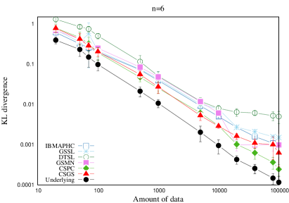
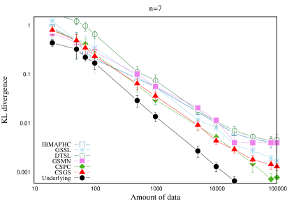
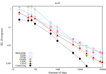
Figure 1: KL divergences over increasing amounts of data for structures learned by several learning algorithms. For comparison reasons, the KL divergence of the underlying structure is shown. Every point represents the average and standard deviation over ten datasets with a fixed size. Lower values indicate better accuracy.

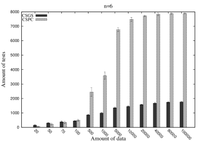
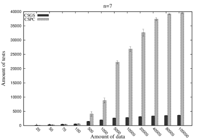
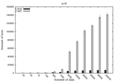
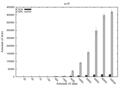
Figure 2: Number of tests performed by CSGS and CSPC for learning structures over increasing amounts of data. Every bar represents the average and standard deviation over ten datasets with a fixed size.

5 Conclusions and future work

In this work we presented CSGS, a new knowledge discovery algorithm for learning Markov network structures by using canonical models. CSGS is similar to the CSPC algorithm [3], except that CSGS uses an alternative search strategy called Grow-Shrink [12, 1], that avoids performing unnecessary independence tests. We evaluated our algorithm against CSPC and several state-of-the-art learning algorithms on synthetic datasets. In our results, CSGS learned structures with similar accuracy to CSPC but performing a reduced number of tests. The directions of future work are focused on further reducing the computational complexity and improving the quality of the learned structures using alternative search strategies. For instance, IBMAP-HC on the side of knowledge discovery algorithms [15], and GSSL on the side of density estimation algorithms [4].

References

- [1] Bromberg, F., Margaritis, D., Honavar, V.: Efficient Markov network structure discovery using independence tests. Journal of Artificial Intelligence Research 35(2), 449 (2009)
- [2] Edera, A., Schlüter, F., Bromberg, F.: Learning markov networks with context-specific independences. In: The 25th International Conference on Tools with Artificial Intelligence, Herndon, VA, USA, November 4-6, 2013. pp. 553–560. IEEE (2013)
- [3] Edera, A., Schlüter, F., Bromberg, F.: Learning Markov networks structures constrained by context-specific independences. viXra submission 1405.0222v1 (2014), http://viXra.org/abs/1405.0222
- [4] Haaren, J.V., Davis, J.: Markov network structure learning: A randomized feature generation approach. In: Proceedings of the Twenty-Sixth National Conference on Artificial Intelligence. AAAI Press (2012)
- [5] Hammersley, J.M., Clifford, P.: Markov fields on finite graphs and lattices. Unpublished manuscript (1971)
- [6] Højsgaard, S.: Yggdrasil: a statistical package for learning split models. In: Proceedings of the Sixteenth conference on Uncertainty in artificial intelligence. pp. 274–281. Morgan Kaufmann Publishers Inc. (2000)
- [7] Højsgaard, S.: Statistical inference in context specific interaction models for contingency tables. Scandinavian journal of statistics 31(1), 143–158 (2004)
- [8] Koller, D., Friedman, N.: Probabilistic Graphical Models: Principles and Techniques. MIT Press, Cambridge (2009)
- [9] Lauritzen, S.L.: Graphical models. Oxford University Press (1996)
- [10] Lowd, D., Davis, J.: Learning Markov network structure with decision trees. In: Data Mining (ICDM), 2010 IEEE 10th International Conference on. pp. 334–343. IEEE (2010)
- [11] Lowd, D., Davis, J.: Improving markov network structure learning using decision trees. Journal of Machine Learning Research 15, 501–532 (2014), http://jmlr.org/papers/v15/lowd14a.html
- [12] Margaritis, D., Thrun, S.: Bayesian network induction via local neighborhoods. Tech. rep., DTIC Document (2000)
- [13] Moore, A., Lee, M.S.: Cached Suficient Statistics for Efficient Machine Learning with Large Datasets. Journal of Artificial Intelligence Research 8, 67–91 (1998)
- [14] Pearl, J.: Probabilistic Reasoning in Intelligent Systems: Networks of Plausible Inference. Morgan Kaufmann Publishers, Inc., 1re edn. (1988)
- [15] Schlüter, F., Bromberg, F., Edera, A.: The IBMAP approach for Markov network structure learning. Annals of Mathematics and Artificial Intelligence pp. 1–27 (2014), http://dx.doi.org/10.1007/s10472-014-9419-5
- [16] Smith, V.A., Yu, J., Smulders, T.V., Hartemink, A.J., Jarvis, E.D.: Computational inference of neural information flow networks. PLoS computational biology 2(11), e161 (2006)