Field operator transformations in Quantum Optics using a novel graphical method with applications to beam splitters and interferometers

Abstract

In this paper we describe a novel, graphical method, allowing the fast computation of field operator transformations for linear lossless optical devices in Quantum Optics (QO). The advantage of this method grows with the complexity of the considered optical setup. As case studies we examine the field operator transformations for the beam splitter (BS), the Mach-Zehnder interferometer (MZI) and the double MZI. We consider the simple case with monochromatic input light, as well as extensions to the non-monochromatic case.

1 Introduction

The quantum optical description of simple optical systems Leo03 allows one to compute and predict the behavior of both classical and non-classical states of light. The beam splitter (BS) is one of the most widely used devices in optical experiments. In the classical description of a lossless BS, energy conservation imposes the relation between input and output electric fields Lou03 ; Gry10 (also known as the Stokes relations). In the quantum optical description Yur86_Cam89 ; Fea87 ; Pra87 , fields are replaced by operators. Starting from Schwinger’s work on the angular momentum operators, general frameworks have been developed, where beam-splitters are described in SU(2) symmetries Yur86_Cam89 . However, authors typically focus on a subset of this general model, having symmetrical Lou03 ; Ger04 ; Fea87 or non-symmetrical operator input-output operator relations Gry10 ; Man95 .

Beam splitters proved to be pivotal in experiments performed in QO, for example by helping differentiate between a coherent and a Fock state Gra86 ; Asp91 and reveal non-classical features of light Kim77_Gho87 ; HOM87_Kim00_Pit96_Kim03 . Applying a coherent state Gla63 ; Sud63 ; Gla63b at one input and a single-quantum Fock state at the other one of a BS allows measuring quantum states of light using the homodyne detector Yue78_Yue83 ; Leo95 .

A Mach-Zehnder interferometer (MZI) is a device composed of two beam splitters and two mirrors Lou03 ; Man95 ; Ger04 . Its versatility has led to its use in countless experiments Gra86 ; Rar90 ; Fra91 ; Kwi95 . With a single light quantum at one input, the rate of photo-detection at its outputs oscillates as the path-length difference of the interferometer is swept Gra86 . Applying pairs of light quanta at its inputs, specific non-classical effects show up Rar90 .

The description of the output states of a BS with given (especially non-classical) input states stirred a lot of interest. Kim et al. Kim02 consider a BS with a variety input states, conjecturing that an entangled output state needs a non-classical input state. The proof was given through a theorem in Xia02 . The transformation relation of field operators for beam splitters has been considered in Ou87 , where a formal solution is given using the P-representation of coherent states and the optical equivalence theorem. The two-photon interference at the output of lossless beam splitters has been thoroughly discussed by Fearn and Loudon Fea89 . Campos et al. Cam90 extend this discussion with a special emphasis on the fourth-order interference applied to lossless optical systems (BS and MZI). Other authors studied more specific scenarios, for example displaced Fock states Win11 or output photon statistics for input squeezed light Pla94 .

The computation of input-output operator relations for optical devices comprising beam splitters and interferometers is traditionally composed of a cascade of successive operator transformations. However, the complexity of these operations grows with the number of cascaded devices in the system. Moreover, due to this calculatory complexity, a good deal of physical insight is lost.

The purpose of this paper is to introduce a graphical method allowing the fast computation of these field operator transformations. Moreover, contrary to the traditional iterative method, all computations remain very intuitive because of the direct physical meaning that can be attached to them. The input light is considered in both the monochromatic and in the more complicated, the non-monochromatic case.

This paper is organized as follows. In Section 2 we give a theoretical motivation for the computation of the field operator transformations. In Section 3, using the newly introduced graph-based method, field operator transformations are computed for a beam splitter and a Mach-Zehnder interferometer. In Section 4 the same transformations are computed for a double Mach-Zehnder interferometer. Finally, conclusions are drawn in Section 5.

2 State and field operator transformations in Quantum Optics

Quite often, interesting devices in QO have two input ports (e.g. beam splitter, MZI). We shall label them with the indexes $0$ and $1$. For simplification, we also assume two output ports, labelled $N$ and $N+1$. We assume linear and lossless optical systems.

If the input is in a pure state, and moreover, if we assume monochromatic light quanta, we can write the input state vector of our system as

$$|\psi_{in}\rangle=f\left(\hat{a}_{0}^{\dagger},\hat{a}_{1}^{\dagger}\right)|0\rangle$$ (1)

where $f$ is an operator function to be determined, $\hat{a}_{k}^{\dagger}$ is the creation operator for the port $k$ (with $k=0,1$) and $|0\rangle$ denotes the vacuum state. For example, if we input the Fock state ${|\psi_{in}\rangle=|0_{0}1_{1}\rangle=\hat{a}_{1}^{\dagger}|0\rangle}$ we find ${f\left(\hat{a}_{0}^{\dagger},\hat{a}_{1}^{\dagger}\right)=\hat{a}_{1}^{\dagger}}$. For a coherent state ${|\psi_{in}\rangle=|0_{0}\alpha_{1}\rangle=\hat{D}_{1}\left(\alpha\right)|0\rangle}$ (where $\hat{D}_{1}\left(\alpha\right)=\text{e}^{\alpha\hat{a}_{1}^{\dagger}-\alpha^{*}\hat{a}_{1}}$ is the displacement operator Gla63 acting on input port $1$), after normally ordering we have

$$f\left(\hat{a}_{0}^{\dagger},\hat{a}_{1}^{\dagger}\right)=\text{e}^{-\frac{|\alpha|^{2}}{2}}\sum_{k=0}^{\infty}{\frac{1}{k!}\left(\alpha\hat{a}_{1}^{\dagger}\right)^{k}}$$ (2)

If one wishes to find the output state, the fact that an input vacuum state transforms into an output vacuum state can always be used, no matter how complicated the system is. Therefore, if we could find the operator functions $g_{0}$ and $g_{1}$ so that

$$\hat{a}_{0}^{\dagger}=g_{0}\left(\hat{a}_{N}^{\dagger},\hat{a}_{N+1}^{\dagger}\right)$$ (3)

and

$$\hat{a}_{1}^{\dagger}=g_{1}\left(\hat{a}_{N}^{\dagger},\hat{a}_{N+1}^{\dagger}\right)$$ (4)

then, at least formally, the output state can be written as

$$|\psi_{out}\rangle=f\left(g_{0}\left(\hat{a}_{N}^{\dagger},\hat{a}_{N+1}^{\dagger}\right),g_{1}\left(\hat{a}_{N}^{\dagger},\hat{a}_{N+1}^{\dagger}\right)\right)|0\rangle$$ (5)

We may call this formalism “the Schrödinger picture”, since the state vector evolves i.e. $|\psi_{in}\rangle\to|\psi_{out}\rangle$. Extension to density matrices instead of state vectors can be readily done.

In most cases, however, the input light is not (or cannot be approximated to be) monochromatic. Therefore, the extension to multi-mode fields is needed. We will be using a narrowband continuous-mode extension, already considered in the literature Cam90 ; Blo90 ; Leg03 . We assume a Heisenberg picture with

$$\hat{E}_{j}^{(+)}\left(\omega\right)=\tilde{\zeta}_{j}\left(\omega\right)\hat{a}_{j}$$ (6)

representing the frequency-domain distribution of the output positive frequency electric field operator and we denoted ${j=N,N+1}$. We also assume that these operator functions can be Fourier transformed in order to obtain their time-domain counterparts $\hat{E}_{N}^{(+)}\left(t\right)$ and $\hat{E}_{N+1}^{(+)}\left(t\right)$ (via the Fourier transform) as

$$\hat{E}^{(+)}_{j}\left(t\right)=\frac{1}{\sqrt{2\pi}}\int{\tilde{\zeta}_{j}\left(\omega\right)\hat{a}_{j}\text{e}^{i\omega{t}}\text{d}\omega}=\zeta_{j}\left(t\right)\hat{a}_{j}$$ (7)

where $j=N,N+1$. We also state a result from the Fourier theory Coh95 that will be used throughout this paper, namely the delay theorem. If a given function $\xi\left(t\right)$ has the Fourier transform $\tilde{\xi}\left(\omega\right)$, then $\tilde{\xi}\left(\omega\right)\text{e}^{-i\omega{\tau}}$ corresponds in the time-domain to a delayed version $\xi\left(t-\tau\right)$ i.e.

$$\frac{1}{\sqrt{2\pi}}\int{\text{e}^{-i\omega{\tau}}\tilde{\xi}\left(\omega\right)\text{e}^{i\omega{t}}\text{d}\omega}=\xi\left(t-\tau\right)$$ (8)

Quite often, the coincidence/singles detection probabilities at the output ports $N$ and/or $N+1$ are needed. For example, if ideal photo-detectors are assumed, the singles detection rate at the output port $N$ between the times $t$ and $t+\text{d}t$ is given by

$$P_{N}\left(t\right)=\langle\psi_{out}|\hat{E}_{N}^{(-)}\left(t\right)\hat{E}_{N}^{(+)}\left(t\right)|\psi_{out}\rangle\qquad$$

$$\qquad=\|\hat{E}_{N}^{(+)}\left(t\right)|\psi_{out}\rangle\|^{2}$$ (9)

where $\hat{E}_{N}^{(-)}\left(t\right)=\left[\hat{E}_{N}^{(+)}\left(t\right)\right]^{\dagger}$. If we suppose that the field operator $\hat{E}_{N}^{(+)}\left(t\right)$ can be written in respect with the input field operators as

$$\hat{E}_{N}^{(+)}\left(t\right)=g_{N}\left(\hat{E}_{0}^{(+)}\left(t\right),\hat{E}_{1}^{(+)}\left(t\right)\right)$$ (10)

and since we chose the Heisenberg picture where state vectors do not change, the singles detection rate from Eq. (2) can be written as

$$P_{N}\left(t\right)=\Big{\|}g_{N}\left(\hat{E}_{0}^{(+)}\left(t\right),\hat{E}_{1}^{(+)}\left(t\right)\right)|\psi_{in}\rangle\Big{\|}^{2}$$ (11)

Similarly, the coincident detection rate at the output ports reads

$$P_{c}\left(t,t+\tau_{d}\right)=\langle\psi_{out}|\hat{E}_{N}^{(-)}\left(t\right)\hat{E}_{N+1}^{(-)}\left(t+\tau_{d}\right)\quad$$

$$\quad\hat{E}_{N+1}^{(+)}\left(t+\tau_{d}\right)\hat{E}_{N}^{(+)}\left(t\right)|\psi_{out}\rangle$$ (12)

and one needs the function $g_{N+1}$ so that

$$\hat{E}_{N+1}^{(+)}\left(t\right)=g_{N+1}\left(\hat{E}_{0}^{(+)}\left(t\right),\hat{E}_{1}^{(+)}\left(t\right)\right)$$ (13)

and therefore the coincidence probability from Eq. (2) can be formally written as

$$P_{c}\left(t,t+\tau_{d}\right)=\Big{\|}g_{N+1}\left(\hat{E}_{0}^{(+)}\left(t+\tau_{d}\right),\hat{E}_{1}^{(+)}\left(t+\tau_{d}\right)\right)$$

$$g_{N}\left(\hat{E}_{0}^{(+)}\left(t\right),\hat{E}_{1}^{(+)}\left(t\right)\right)|\psi_{in}\rangle\Big{\|}^{2}$$ (14)

The interest in finding the operator functions $g_{N}$ and $g_{N+1}$ is now obvious.

Figure 1: The beam splitter described in the graphical method. In the left graph we express the field operators $\hat{a}_{0}^{\dagger}$ and $\hat{a}_{1}^{\dagger}$ in respect with $\hat{a}_{2}^{\dagger}$ and $\hat{a}_{3}^{\dagger}$ while in the right one we express $\hat{a}_{2}$ and $\hat{a}_{3}$ in respect with $\hat{a}_{0}$ and $\hat{a}_{1}$.

3 Applying the graphical method to a beam splitter and to a Mach-Zehnder interferometer

In the following a novel, graphical method allowing the fast computation of field operator transformations will be introduced. In this section we apply this method to a beam splitter and to a Mach-Zehnder interferometer.

For a symmetrical, lossless beam splitter, the output annihilation operators $\hat{a}_{3}$ and $\hat{a}_{2}$ can be written in respect with the input field operators $\hat{a}_{1}$ and $\hat{a}_{0}$ and the transmission ($T$) and reflection ($R$) coefficients (see Fig. 2, beam splitter $\text{BS}_{1}$) a result found in many textbooks (e.g. Lou03 page 214, Ger04 page 138). After some basic manipulations, one easily obtains the input creation field operators in respect with the output ones.

For the graphical method we start by representing the BS with the butterfly-like graph, depicted in Fig. 1 (left graphic). The nodes represent the fields in our points of interest and the arrows have the amplitude coefficients that connect them. The field operator $\hat{a}_{0}^{\dagger}$ is composed of two inverse paths from the output, one from $\hat{a}_{2}^{\dagger}$ with an amplitude $T$ and one from $\hat{a}_{3}^{\dagger}$ with an amplitude $R$ yielding

$$\hat{a}_{0}^{\dagger}=T\hat{a}_{2}^{\dagger}+R\hat{a}_{3}^{\dagger}$$ (15)

and applying the same ideas to $\hat{a}_{1}^{\dagger}$, one quickly obtains

$$\hat{a}_{0}^{\dagger}=R\hat{a}_{2}^{\dagger}+T\hat{a}_{3}^{\dagger}$$ (16)

Similarly, from the right graph of Fig. 1, the output field operators $\hat{a}_{2}$ $\hat{a}_{3}$ can be obtained via two paths from the input ports and, without any surprise, we obtain classical results found in most textbooks.

Extension to the non-monochromatic case can be done using the continuous frequency modes from Eq. (6), yielding

$$\tilde{\zeta_{2}}\left(\omega\right)\hat{a}_{2}=T\tilde{\zeta_{0}}\left(\omega\right)\hat{a}_{0}+R\tilde{\zeta_{1}}\left(\omega\right)\hat{a}_{1}$$ (17)

and

$$\tilde{\zeta_{3}}\left(\omega\right)\hat{a}_{3}=R\tilde{\zeta_{0}}\left(\omega\right)\hat{a}_{0}+T\tilde{\zeta_{1}}\left(\omega\right)\hat{a}_{1}$$ (18)

Denoting $\hat{E}_{k}^{(+)}=\tilde{\zeta_{k}}\left(\omega\right)\hat{a}_{k}$ for $k=2,3$ and performing the inverse Fourier transform of the above equations one obtains the time-domain input-output relations.

For this simple example, the advantage of the graph-based method is not at all obvious. It will, nonetheless, become important when the devices discussed will become more complex.

A Mach-Zehnder interferometer (depicted in Fig. 2) is composed of two beam splitters and two mirrors. We denote again the input (creation) field operators by $\hat{a}_{0}^{\dagger}$ and $\hat{a}_{1}^{\dagger}$. The delay $\varphi_{1}$ introduced in the lower path (i.e. $\text{BS}_{1}$ – $\text{M}_{2}$ – $\text{BS}_{2}$) accounts for the path length difference $\Delta{z}$ between the two arms, i.e. $\varphi_{1}=k\Delta{z}$, where $k$ is the wavenumber. Being at a fixed frequency $\omega=k/c$, we have $\varphi_{1}=\omega\tau_{1}$ where $\tau_{1}=\Delta{z}/c$.

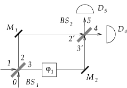
Figure 2: The Mach-Zehnder interferometer. The delay ($\varphi_{1}$) models the path length difference between the two arms of the interferometer.

In the case of the MZI, we construct the graph from Fig. 3, composed of two “butterflies” (for each BS) and the phase shift caused by the path length difference of the two arms by the two horizontal arrows connecting them with amplitudes $1$ and, respectively, $\text{e}^{i\varphi_{1}}$. We model this delay through a positive exponential factor (i.e. $i\varphi_{1}=+i\omega\tau_{1}$) since we are moving “backwards in time”, from the input of $\text{BS}_{2}$ to the output of $\text{BS}_{1}$. The names of the intermediate field operators depicted in Fig. 3 are needed only for explanatory purposes in the example below.

Figure 3: The graph for the computation of the input operators $\hat{a}_{1}^{\dagger}$ and $\hat{a}_{0}^{\dagger}$ in respect with the output field operators $\hat{a}_{4}^{\dagger}$ and $\hat{a}_{5}^{\dagger}$.

In order to illustrate the graphical method, we compute in detail the field operator $\hat{a}_{0}^{\dagger}$ in function of the output field operators $\hat{a}_{4}^{\dagger}$ and $\hat{a}_{5}^{\dagger}$. We note that there are two possible paths connecting $\hat{a}_{4}^{\dagger}$ to $\hat{a}_{0}^{\dagger}$: from $\hat{a}_{4}^{\dagger}$ via $(\hat{a}^{\prime}_{2})^{\dagger}$ and $\hat{a}_{2}^{\dagger}$ to $\hat{a}_{0}^{\dagger}$ with an amplitude $T^{2}$ and no phase shift and from $\hat{a}_{4}^{\dagger}$ via $(\hat{a}^{\prime}_{3})^{\dagger}$ and $\hat{a}_{3}^{\dagger}$ to $\hat{a}_{0}^{\dagger}$ with an amplitude $R^{2}$ and a phase shift $\text{e}^{i\varphi_{1}}$. Another two paths connect $\hat{a}_{5}^{\dagger}$ to $\hat{a}_{0}^{\dagger}$: from $\hat{a}_{5}^{\dagger}$ via $(\hat{a}^{\prime}_{2})^{\dagger}$ and $\hat{a}_{2}^{\dagger}$ to $\hat{a}_{0}^{\dagger}$ with an amplitude $TR$ and no phase shift and from $\hat{a}_{5}^{\dagger}$ via $(\hat{a}^{\prime}_{3})^{\dagger}$ and $\hat{a}_{3}^{\dagger}$ to $\hat{a}_{0}^{\dagger}$ with an amplitude $TR$ and phase shift $\text{e}^{i\varphi_{1}}$. Summing up all these amplitudes takes us to

$$\hat{a}_{0}^{\dagger}=\left(T^{2}+R^{2}\text{e}^{i\varphi_{1}}\right)\hat{a}_{4}^{\dagger}+TR\left(1+\text{e}^{i\varphi_{1}}\right)\hat{a}_{5}^{\dagger}$$ (19)

We obtained straight away this result by the simple inspection of the graph from Fig. 1. Similarly, writing down the amplitudes and phase shifts of the paths connecting $\hat{a}_{1}^{\dagger}$ to $\hat{a}_{4}^{\dagger}$ and $\hat{a}_{5}^{\dagger}$ yields

$$\hat{a}_{1}^{\dagger}=TR\left(1+\text{e}^{i\varphi_{1}}\right)\hat{a}_{4}^{\dagger}+\left(T^{2}\text{e}^{i\varphi_{1}}+R^{2}\right)\hat{a}_{5}^{\dagger}$$ (20)

Figure 4: The (frequency-domain) graph used for the computation of the field operators $\hat{a}_{4}$ and $\hat{a}_{5}$ in respect with the input operators $\hat{a}_{0}$ and $\hat{a}_{1}$ for a Mach-Zehnder interferometer.

If we are interested in the operator functions connecting the output annihilation field operators $\hat{a}_{4}$ and $\hat{a}_{5}$ to the input field operators $\hat{a}_{0}$ and $\hat{a}_{1}$, we construct the “direct” graph for monochromatic light, depicted in Fig. 4. It is composed of two “butterflies” (similar to the one depicted in Fig. 1, right graphic) and a delay line equivalent to a phase shift $\text{e}^{-i\omega\tau_{1}}$ since we are at a fixed frequency. This time the exponent is $-i\omega\tau_{1}$ since we are moving “forward in time”. From the graph depicted in Fig. 4 one can readily write the four amplitudes connecting $\hat{a}_{4}$ to the input field operators, having

$$\hat{a}_{4}=\left(T^{2}+R^{2}\text{e}^{-i\omega\tau_{1}}\right)\hat{a}_{0}+TR\left(1+\text{e}^{-i\omega\tau_{1}}\right)\hat{a}_{1}$$ (21)

and similarly for $\hat{a}_{5}$ yielding

$$\hat{a}_{5}=TR\left(1+\text{e}^{-i\omega\tau_{1}}\right)\hat{a}_{0}+\left(T^{2}\text{e}^{-i\omega\tau_{1}}+R^{2}\right)\hat{a}_{1}$$ (22)

We extend our analysis to continuous multi-mode non-monochromatic light quanta by applying mode functions $\tilde{\zeta}_{0}\left(\omega\right)$ and $\tilde{\zeta}_{1}\left(\omega\right)$ to each input operator. We end up with the input electric field operators $\hat{E}^{(+)}_{0}\left(\omega\right)$ and $\hat{E}^{(+)}_{1}\left(\omega\right)$. Nonetheless, we are interested in a time-domain description, therefore we will perform an inverse Fourier transform $\hat{E}^{(+)}_{k}\left(\omega\right)\rightarrow\hat{E}^{(+)}_{k}\left(t\right)$. Using Eq. (8) any phase shift will become a time delay. We are now able to construct the graph from Fig. 5. The two beam splitters are the same “butterflies” (assumed frequency-independent), however the phase shift from Fig. 4 became a time delay $\tau_{1}$, depicted in Fig. 5 as a rectangle.

One can express now the output field operators in respect with the input ones. The operator $\hat{E}^{(+)}_{4}\left(t\right)$ can be reached from $\hat{E}^{(+)}_{0}\left(t\right)$ via two paths ($T-1-T$ and $R-\text{delay }\tau_{1}-R$). Adding the two possible paths from $\hat{E}^{(+)}_{1}\left(t\right)$ allows one to directly write the result

$$\hat{E}^{(+)}_{4}\left(t\right)=T^{2}\hat{E}^{(+)}_{0}\left(t\right)+R^{2}\hat{E}^{(+)}_{0}\left(t-\tau_{1}\right)\quad$$

$$\quad+TR\hat{E}^{(+)}_{1}\left(t\right)+TR\hat{E}^{(+)}_{1}\left(t-\tau_{1}\right)$$ (23)

and similarly, for the other output field operator

$$\hat{E}^{(+)}_{5}\left(t\right)=TR\hat{E}^{(+)}_{0}\left(t\right)+TR\hat{E}^{(+)}_{0}\left(t-\tau_{1}\right)\quad$$

$$\quad+R^{2}\hat{E}^{(+)}_{1}\left(t\right)+T^{2}\hat{E}^{(+)}_{1}\left(t-\tau_{1}\right)$$ (24)

Figure 5: The (time-domain) graph used for the computation of the output electric field operators $\hat{E}^{(+)}_{4}\left(t\right)$ and $\hat{E}^{(+)}_{5}\left(t\right)$ in respect with the input operators $\hat{E}^{(+)}_{0}\left(t\right)$ and $\hat{E}^{(+)}_{1}\left(t\right)$.

4 Applying the graphical method to a double Mach-Zehnder interferometer

We introduce and discuss in the following a double MZI setup, depicted in Fig. 6. The beam splitters $\text{BS}_{1}$ and $\text{BS}_{2}$ with the two mirrors $\text{M}_{1}$ and $\text{M}_{2}$ form the first MZI. The delay $\varphi_{1}$ models the path length difference. The second MZI is composed of the beam splitters $\text{BS}_{2}$ and $\text{BS}_{3}$, together with the two mirrors $\text{M}_{3}$ and $\text{M}_{4}$. Similarly, the delay $\varphi_{2}$ models the path length difference. It is assumed that, with the corresponding delays taken out of the experiment, each MZI has equal length arms. The photo-detectors $D_{6}$ and $D_{7}$ (assumed ideal) are installed at the two outputs of $\text{BS}_{3}$.

Results concerning the double Mach-Zehnder interferometer have been discussed in detail in Ata14 and will be used in the following as reference.

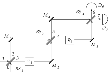
Figure 6: The experiment proposed in Section 4. The first Mach-Zehnder interferometer is composed of the beam splitters $\text{BS}_{1}$ and $\text{BS}_{2}$ together with the mirrors $\text{M}_{1}$ and $\text{M}_{2}$. Similarly, the second Mach-Zehnder interferometer is composed of $\text{BS}_{2}$ , $\text{BS}_{3}$, $\text{M}_{3}$ and $\text{M}_{4}$. The delays ($\varphi_{1}$ and $\varphi_{2}$) model the path length difference in each MZI.

Similar to the previous case studies, we construct a graph, depicted in Fig. 7. Each beam splitter is depicted as a butterfly (with coefficients $T$ and $R$) and the path length difference in each MZI is modelled as a phase shift. We start by expressing the field operator $\hat{a}_{0}^{\dagger}$ in respect with the output field operators. From Fig. 7 one can see that there are four possible paths from $\hat{a}_{6}^{\dagger}$ to $\hat{a}_{0}^{\dagger}$ yielding the amplitudes: $T^{3}\text{e}^{i\varphi_{2}}$, $TR^{2}$, $TR^{2}\text{e}^{i(\varphi_{1}+\varphi_{2})}$ and $TR^{2}\text{e}^{i\varphi_{1}}$. Likewise, there are four paths from $\hat{a}_{7}^{\dagger}$ to $\hat{a}_{0}^{\dagger}$. Therefore, the input operator $\hat{a}_{0}^{\dagger}$ in respect with the output operators $\hat{a}_{6}^{\dagger}$ and $\hat{a}_{7}^{\dagger}$ can be directly written yielding

$$\hat{a}_{0}^{\dagger}=\left(T^{3}\text{e}^{i\varphi_{2}}+TR^{2}+TR^{2}\text{e}^{i(\varphi_{1}+\varphi_{2})}+TR^{2}\text{e}^{i\varphi_{1}}\right)\hat{a}_{6}^{\dagger}$$

$$+\left(R^{3}\text{e}^{i(\varphi_{1}+\varphi_{2})}+T^{2}R\text{e}^{i\varphi_{1}}+T^{2}R\text{e}^{i\varphi_{2}}+T^{2}R\right)\hat{a}_{7}^{\dagger}\quad$$ (25)

Similar arguments allow us to directly write the input operator $\hat{a}_{1}^{\dagger}$ in respect with the output ones,

$$\hat{a}_{1}^{\dagger}=\left(T^{2}R\text{e}^{i\varphi_{2}}+R^{3}+T^{2}R\text{e}^{i(\varphi_{1}+\varphi_{2})}+T^{2}R\text{e}^{i\varphi_{1}}\right)\hat{a}_{6}^{\dagger}$$

$$+\left(T^{3}\text{e}^{i\varphi_{1}}+TR^{2}\text{e}^{i(\varphi_{1}+\varphi_{2})}+TR^{2}\text{e}^{i\varphi_{2}}+TR^{2}\right)\hat{a}_{7}^{\dagger}\quad$$ (26)

Eqs. (4) and (4) could have been found using the traditional, iterative method Ata14 . The graphical method, however, gave these results faster and in a more intuitive way.

Figure 7: The (frequency domain) graph used to compute the input field operators $\hat{a}_{0}^{\dagger}$ and $\hat{a}_{1}^{\dagger}$ in respect with the output field operators $\hat{a}_{6}^{\dagger}$ and $\hat{a}_{7}^{\dagger}$ for a double Mach-Zehnder interferometer.

Extension to non-monochromatic light quanta can be done using the same path as before. Therefore, we construct the graph from Fig. 8. One can express now the output field operator $\hat{E}^{(+)}_{6}\left(t\right)$ in respect with the input electric field operators $\hat{E}^{(+)}_{0}\left(t\right)$ and $\hat{E}^{(+)}_{1}\left(t\right)$ by simply inspecting the graph. We have four possible paths connecting $\hat{E}^{(+)}_{0}\left(t\right)$ to $\hat{E}^{(+)}_{6}\left(t\right)$ yielding the amplitudes and delays: $T^{3}$ with a delay of $\tau_{2}$, $TR^{2}$ with a delay of $\tau_{1}$, $TR^{2}$ with no delay and finally $R^{3}$ with a delay of $\tau_{1}+\tau_{2}$. Adding the contribution from $\hat{E}^{(+)}_{1}\left(t\right)$ yields the final expression

$$\hat{E}^{(+)}_{6}\left(t\right)=T^{3}\hat{E}^{(+)}_{0}\left(t-\tau_{2}\right)+TR^{2}\hat{E}^{(+)}_{0}\left(t-\tau_{1}\right)\quad$$

$$+TR^{2}\hat{E}^{(+)}_{0}\left(t-\tau_{1}-\tau_{2}\right)+TR^{2}\hat{E}^{(+)}_{0}\left(t\right)$$

$$+T^{2}R\hat{E}^{(+)}_{1}\left(t-\tau_{1}\right)+T^{2}R\hat{E}^{(+)}_{1}\left(t-\tau_{1}-\tau_{2}\right)$$

$$+T^{2}R\hat{E}^{(+)}_{1}\left(t-\tau_{2}\right)+R^{3}\hat{E}^{(+)}_{1}\left(t\right)$$ (27)

Considering the four paths from $\hat{E}^{(+)}_{0}\left(t\right)$ and the other four from $\hat{E}^{(+)}_{1}\left(t\right)$ to $\hat{E}^{(+)}_{7}\left(t\right)$ one finds

$$\hat{E}^{(+)}_{7}\left(t\right)=T^{2}R\hat{E}^{(+)}_{0}\left(t-\tau_{2}\right)+T^{2}R\hat{E}^{(+)}_{0}\left(t-\tau_{1}\right)$$

$$+T^{2}R\hat{E}^{(+)}_{0}\left(t\right)+R^{2}\hat{E}^{(+)}_{0}\left(t-\tau_{1}-\tau_{2}\right)$$

$$+T^{3}\hat{E}^{(+)}_{1}\left(t-\tau_{1}\right)+TR^{2}\hat{E}^{(+)}_{1}\left(t-\tau_{1}-\tau_{1}\right)$$

$$+TR^{2}\hat{E}^{(+)}_{1}\left(t\right)+TR^{2}\hat{E}^{(+)}_{1}\left(t-\tau_{2}\right)$$ (28)

Eqs. (4) and (4) were also obtained with merely a visual inspection of the graph depicted in Fig. 8. They are identical to the results from Ata14 but the effort in obtaining them was much lower.

Figure 8: The (time-domain) graph for the computation of the output operators $\hat{E}^{(+)}_{6}\left(t\right)$ and $\hat{E}^{(+)}_{7}\left(t\right)$ in respect with the input ones, $\hat{E}^{(+)}_{0}\left(t\right)$ and $\hat{E}^{(+)}_{1}\left(t\right)$.

5 Conclusions

In this paper we introduced and discussed a graphical method allowing the easy computation of field operator transformation for linear lossless devices in quantum optics comprising beam splitters and interferometers. Besides the advantage in the speed of calculation, this method offers an intuitive physical interpretation: operators transform via a sum of probability amplitudes from each available path in the considered optical system. Direct and inverse graphs can be built in function of the required operator equation. Extension to the non-monochromatic case is done via time-domain graphs, where the output electric field operators can be computed in respect with the input ones in the same, intuitive, graphical manner.

References

- (1) U. Leonhardt, Rep. Prog. Phys. 66, 1207 (2003)
- (2) R. Loudon, The Quantum Theory of Light, (Oxford University Press, Third Edition, 2003)
- (3) G. Grynberg, A. Aspect, C. Fabre, Introduction to Quantum Optics: From the Semi-classical Approach to Quantized Light, (Cambridge University Press, 2010)
- (4) L. Mandel, E. Wolf, Optical Coherence and Quantum Optics, (Cambridge, 1995)
- (5) C. Gerry , P. Knight, Introductory Quantum Optics, (Cambridge, 2004)
- (6) B. Yurke, S. McCall, J. Klauder, Phys. Rev. A, 33, 4033 (1986); R. Campos, B. Saleh, M. Teich, Phys. Rev. A, 40, 1371 (1989)
- (7) H. Fearn, R. Loudon, Opt. Comm., 64, 485 (1987)
- (8) S. Prasad, M. Scully, W. Martiessen, Opt. Comm., 62, 139 (1987)
- (9) P. Grangier, G. Roger, A. Aspect, Europhys. Lett., 1, 173 (1986)
- (10) A. Aspect, P. Grangier, One-Photon Light Pulses versus Attenuated Classical Light Pulses in “International Trends in Optics”, 247, J. W. Goodman ed., (Academic Press, 1991)
- (11) H. Kimble, M. Dagenais, L. Mandel, Phys. Rev. Lett. 39, 691 (1977); R. Ghosh, L. Mandel, Phys. Rev. Lett. 59, 1903 (1987)
- (12) C. Hong, Z. Ou, L. Mandel, Phys. Rev. Let. 59, 2044 (1987); Y-H. Kim, R. Yu, S. Kulik, Y. Shih, M. Scully, Phys. Rev. Lett. 84, 1 (2000); T. Pittman et al., Phys. Rev. Let. 77, 1917 (1996); Y.-H. Kim, Phys. Lett. A, 315, 352 (2003)
- (13) R. Glauber, Phys. Rev. 130, 2259 (1963)
- (14) E. Sudarshan, Phys. Rev. Lett. 10, 277 (1963)
- (15) R. Glauber, Phys. Rev. 131, 2766 (1963)
- (16) H. Yuen, J. Shapiro, in Coherence and Quantum Optics IV, L. Mandel and E. Wolf, eds. 719 (Plenum, 1978); H. Yuen, V. Chan, Opt. Lett., 8, 177 (1983)
- (17) U. Leonhardt, H. Paul, Prog. Quant. Electr. 19, 89 (1995)
- (18) J. Rarity et al., Phys. Rev. Lett. 65, 1348 (1990)
- (19) J. Franson, Phys. Rev. A, 44, 4552 (1991)
- (20) P. Kwiat et al., Phys. Rev. Lett. 74, 4763 (1995)
- (21) M. Kim, W. Son, V. Bužek, P. Knight, Phys. Rev. A, 65, 032323 (2002) arXiv:quant-ph/0106136
- (22) W. Xiang-bin, Phys. Rev. A, 66, 024302 (2002) arXiv:quant-ph/0204039
- (23) Z. Ou, C. Hong, L. Mandel, Opt. Comm., 63, 118 (1987)
- (24) H. Fearn, R. Loudon, J. Opt. Soc. Am. B, 6, 917 (1989)
- (25) R. Campos, B. Saleh, M. Teich, Phys. Rev. A, 42, 4127 (1990)
- (26) A. Windlager et al, Opt. Comm., 284, 1907 (2011)
- (27) R. van der Plank, L. Suttorp, Opt. Comm., 112, 145 (1994)
- (28) K. Blow, R. Loudon, S. Phoenix, T. Shepherd, Phys. Rev. A 42, 4102 (1990)
- (29) T. Legero, T. Wilk, A. Kuhn, G. Rempe, Appl. Phys. B 77, 797 (2003) arXiv:quant-ph/0308024
- (30) L. Cohen, Time-frequency Analysis, (Prentice Hall, 1995)
- (31) S. Ataman, arXiv:1407.1704