Genus Distributions
of Cubic Series-Parallel Graphs

Abstract.

We derive a quadratic-time algorithm for the genus distribution of any 3-regular, biconnected series-parallel graph, which we extend to any biconnected series-parallel graph of maximum degree at most 3. Since the biconnected components of every graph of treewidth 2 are series-parallel graphs, this yields, by use of bar-amalgamation, a quadratic-time algorithm for every graph of treewidth at most 2 and maximum degree at most 3.

Version: 06:32  

1. Introduction

For $i=0,1,2,\ldots$, let $g_{i}(G)$ be the number of topologically distinct cellular embeddings of the graph $G$ in the orientable surface $S_{i}$ of genus $i$. The genus distribution of the graph $G$ is the sequence of numbers

(1.1) $$g_{i}(G):i=0,1,\ldots$$

By the interpolation principle (see Theorem 3.4.1 of [GrTu87] or Theorem 4.5.3 of [MoTh01]), the set $\{i:g_{i}(G)>0\}$ is a set of consecutive integers. The smallest number in this set is the minimum genus of the graph $G$, and the largest is the maximum genus of $G$.

The main focus of this paper is the derivation of a quadratic-time algorithm for the genus distribution of any 3-regular, biconnected series-parallel graph. This algorithm is readily extended to a quadratic-time algorithm for the genus distribution of any graph of treewidth at most 2 and maximum degree at most 3. The simplicity with which this specialized algorithm can be implemented, or applied by hand with the aid of a spreadsheet, distinguishes it from the recently derived quadratic-time algorithm [Gr14] for the genus distribution of any class of graphs of fixed treewidth and bounded degree.

Basic results on genus distribution

Five fundamental papers [GKP10, Gr11a, PKG10, KPG10, PKG12] of the first author and his co-authors Khan and Poshni have established methods for calculating the genus distribution of a graph that is constructed by various kinds of amalgamation of graphs of known genus distribution. These methods involve partitioned genus distributions and productions. In order to develop an algorithm for a specific class of graphs, the starting point is to formulate a recursive specification of the graphs in that class, in which the operations used to create larger graphs from smaller graphs are varieties of amalgamation or self-amalgamation. Then methods similar to those of the five fundamental papers are used to calculate the genus distribution recursively. This paradigm was used successfully in calculating the genus distributions of 3-regular outerplanar graphs [Gr11b], of 4-regular outerplanar graphs [PKG11], of Halin graphs [Gr13], and of the $3\times n$-mesh graphs [KPG12]. We adopt the same paradigm in this paper.

Connections of treewidth to embedding problems

Since the introduction of the concept of treewidth by Robertson and Seymour, bounding the treewidth has been widely used to obtain polynomial-time algorithms for problems that are otherwise NP-hard. In particular, deciding whether an arbitrarily selected graph can be embedded in a given surface is NP-complete [Th89]; however, for any class of graphs of bounded treewidth, Kawarabayashi, Mohar, and Reed [KMR09] have derived a linear-time algorithm for calculating the minimum genus.

Although outerplanar graphs have treewidth 2, and although Halin graphs and $P_{3}\times P_{n}$ meshes have treewidth 3 (see [Bo98]), decomposition trees have not occurred in the calculation of specific genus distributions in any papers as yet. Nonetheless, low treewidth plays an implicit role in the recursive specification of the family of graphs in each of those papers. Similarly, in the present paper, low treewidth plays an implicit role, since it allows for a simple recursive construction of the graphs under consideration.

Terminology

In what follows, a graph is taken to be connected and devoid of self-loops, unless something else can be inferred from the immediate context. Multi-edges are to be expected. We use $V_{G}$ and $E_{G}$ to denote the vertex set and edge set of a graph $G$. A connected graph is biconnected if it has no cutpoints.

The embeddings in this paper are cellular embeddings in oriented surfaces. The terminology used here is predominantly consistent with [GrTu87] and [BWGT09]. See also [MoTh01], for a slightly different approach. We abbreviate “face-boundary walk” as fb-walk.

A two-terminal series-parallel graph is a doubly vertex-rooted graph $(G,p,q)$, as per the following recursive definition.

$B$:

The graph $(K_{2},p,q)$ is a two-terminal series-parallel graph, where $p$ and $q$ are the vertices of $K_{2}$, called the source root and the target root, respectively.

$R_{1}$:

series operation $(G,p,q)\odot_{s}(G^{\prime},p^{\prime},q^{\prime})$ Target root $q$ of $G$ is merged with source root $p^{\prime}$ of $G^{\prime}$. The amalgamated graph $G\odot_{s}G^{\prime}$ with roots $p$ and $q^{\prime}$, as in Figure 1.1(a), is a two-terminal series-parallel graph.

$R_{2}$:

parallel operation $(G,p,q)\odot_{p}(G^{\prime},p^{\prime},q^{\prime})$ The result of merging source root $p$ with source root $p^{\prime}$ , and also merging target root $q$ with target root $q^{\prime}$, as in Figure 1.1(b), is a two-terminal series-parallel graph.

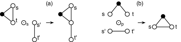
Figure 1.1. Operations on series-parallel graphs.

A graph $G$ is a series-parallel graph if there is a choice of terminals $p$ and $q$ such that $(G,p,q)$ is a two-terminal series-parallel graph. Our definition here is consistent with that of [Bo98] and [Ep92]. A third operation, called a jackknife operation is allowed by [BPT09], and the resulting class of graphs that they call “series-parallel” is equivalent to that of [Du65] — see Remark 8.1 of [BPT09]. The “series-parallel graphs” in [Du65] are identified there as the graphs with no embedded “Wheatstone bridge” (which is Duffin’s terminology for a $K_{4}$ topological minor). These are precisely the graphs that have no $K_{4}$-minor (e.g., see Proposition 1.7.2 of [Die06]). According to Theorem 17 of [Bo98], the graphs without a $K_{4}$-minor are exactly the graphs of treewidth at most 2. It follows that our extended genus-distribution algorithm can be applied to any of them in quadratic time, and that we do not need to further explore the distinctions between the varying definitions of “series-parallel graphs”.

Outline of this paper

Section 2 derives a characterization of 3-regular, biconnected series-parallel graphs that facilitates the genus distribution algorithm for that family of graphs. Section 3 introduces the concepts of partitioned genus distributions and productions. The top-level description of an algorithm for the genus distribution of any 3-regular, biconnected series-parallel graph is given in Section 4. Sections 5 and 6 derive the productions needed to complete the calculation, as well as their application to calculating the genus distribution of an illustrative example. Section 6 also gives proof that the algorithm runs in quadratic time. Section 7 extends the algorithm to all graphs of treewidth 2 and maximum degree 3.

This paper is almost entirely self-contained, except for some details of the well-established concept of partitioned genus distributions and of the methods (as in [GKP10] and [PKG10]) for constructing productions (which are quite necessary for the algorithm). Prior experience with calculating genus distributions of graph amalgamations, especially as in [Gr11b] and [Gr13], is likely to be quite helpful.

2. Cubic Biconnected Series-Parallel Graphs

The dipole $D_{n}$ is the graph with two vertices and an $n$-fold multi-edge joining them. In this section, we prove that every 3-regular, biconnected series-parallel graph can be obtained by iterated application of the following operation to the dipole $D_{3}$.

$\tau$:

Trisect an arbitrary edge $e$ of a graph $G$ and install a new edge in parallel to the “middle third” of edge $e$.

This operation, which is applicable to an non-empty graph, is called a dmt-step (“dmt” is an abbreviation of “double the middle third”), is illustrated by Figure 2.1.

Figure 2.1. A dmt-step: double the middle third.

We define a second operation, which is applicable to 3-regular multigraphs, other than the dipole $D_{3}$.

$\tau^{-1}$:

In a 3-regular graph $G$, let $d$ and $e$ be edges that share the same two endpoints, $u$ and $v$, and in which no other edge shares these two endpoints. Delete edge $d$, and then smooth away vertices $u$ and $v$.

We observe that the operation $\tau^{-1}$ can be used as an inverse to the operation $\tau$.

The proof of our characterization of 3-regular, biconnected series-parallel graphs uses the following four propositions.

Proposition 2.1.

A graph $G$ has treewidth at most 2 if and only if every biconnected component of $G$ is a series-parallel graph.

Proof.

This is Theorem 42 of [Bo98]. ∎

Proposition 2.2.

A graph $G$ has treewidth at most 2 if and only if contains no $K_{4}$-minor.

Proof.

This follows immediately from Theorem 17 of [Bo98]. ∎

Proposition 2.3.

Let $G$ be a 3-regular, biconnected series-parallel graph, and let $G^{\prime}$ be a graph with at least two vertices, obtained by applying operation $\tau^{-1}$ to edges $d$ and $e$ of $G$ , with shared endpoints $u$ and $v$. Then $G^{\prime}$ is 3-regular, biconnected, and series-parallel.

Proof.

Since $G$ is 3-regular, all of its vertices are 3-valent. The operation $\tau^{-1}$ eliminates two vertices of $G$ without changing the valences of the remaining vertices. Thus, the graph $G^{\prime}$ is 3-regular.

Let $x$ and $y$ be any two vertices of $G^{\prime}$. Since $G$ is biconnected, there is a pair of internally disjoint paths in $G$ joining $x$ and $y$, by Menger’s theorem. If one of these paths contains either of the vertices $u$ or $v$, then it also contains one of the edges $d$ or $e$, since $G$ is 3-regular, and the other path contains neither vertex $u$ nor vertex $v$. Thus the images of the two internally disjoint path in $G$ are two internally disjoint paths in $G^{\prime}$. Hence, the graph $G^{\prime}$ is biconnected.

Since the graph $G$ is series-parallel, its treewidth is at most 2, by Proposition 2.1. It follows from Proposition 2.2 that $G$ has no $K_{4}$-minor. Accordingly, the graph $G^{\prime}$ has no $K_{4}$ minor. Therefore, by Proposition 2.2, the graph $G^{\prime}$ has treewidth at most 2. We conclude from Proposition 2.1 that the graph $G^{\prime}$ is series-parallel. ∎

Proposition 2.4 (Dirac’s theorem).

Let $G$ be a biconnected simple graph of minimum degree 3. Then $G$ contains a subgraph that is homeomorphic to the complete graph $K_{4}$.

Proof.

This is a theorem of [Dir52]. ∎

Theorem 2.5.

Let $G$ be a biconnected 3-regular series-parallel graph. Then there exist vertices $p,q\in V_{G}$ such that the two-terminal series-parallel graph $(G,p,q)$ is derivable from $(D_{3},p,q)$ by a sequence of applications of the operation $\tau$.

Proof.

Let $H$ be a smallest graph obtainable by iterative application of operation $\tau^{-1}$ to the graph $G$, that is, a graph such that no pair of vertices is joined by exactly two edges. By Proposition 2.3, the graph $H$ is 3-regular, biconnected, and series-parallel. We observe that $H$ cannot be simple, lest it contain, by Dirac’s theorem, a homeomorphic copy of $K_{4}$, a contradiction, in view of Propositions 2.2 and 2.1. Accordingly, there is a pair of vertices $p,q\in V_{H}$ with at least two edges joining them. Since there cannot be exactly two edges joining $p$ and $q$, by the minimality of the graph $H$, and since $H$ is 3-regular, it follows that $H\cong D_{3}$. Reversing the sequence of $\tau^{-1}$-operations, we obtain a derivation of $(G,p,q)$ from $(D_{3},p,q)$ by iterative application of the operation $\tau$. ∎

We define a dmt-string to be a graph obtained by iterative application of dmt-steps to the graph $K_{2}$. We observe that each dmt-string has two univalent vertices and that all other vertices are trivalent.

Corollary 2.6.

Let $(G,p,q)$ be a 3-regular, biconnected two-terminal series-parallel graph. Then $(G,p,q)$ can be represented by a set of three dmt-strings, each with a univalent $p$-vertex and a univalent $q$-vertex, from which $(G,p,q)$ is formed by two parallel operations.

3. Partials and Productions

When calculating the genus distribution of a family of graphs, we commonly use a finer partition of the embeddings during the intermediate steps. For computational purposes, we need to isolate subsets of embeddings upon which the surgical operations used in the recursive construction of that family have the same effect. Whereas the genus distribution of a graph is an inventory according only (as per (1.1)) to the genus of the embedding surface, a partitioned genus distribution refines the genus distribution of a rooted graph, according to the incidence of fb-walks on the roots, which is the critical factor in the behavior of a surgical operation on an embedding. In other words, a partitioned genus distribution is a partition of all embeddings of the graph with a given genus into into several types, which allows us to keep under control the structure of the faces incident with the roots before, respectively after the amalgamation. The cells of the finer partition are called partials. In this context, we sometimes abbreviate genus distribution as gd and partitioned genus distribution as pgd.

Calculating the genus distributions of 3-regular series-parallel graphs involves amalgamating subgraphs at pairs of terminals, such that the sum of the degrees of an amalgamated pair of vertices is at most 3. Thus, the possible degrees of the terminals prior to the final operation are 1 and 2. When both terminals are univalent, the genus distribution of $(G,p,q)$ is partitioned into the following partials:

$$uu_{i}^{\bullet}(G,p,q) = G\to S_{i}$$ the number of embeddings such that

terminals $$p q$$ and do not occur on the same fb-walk;

$$uu_{i}^{\prime}(G,p,q) = G\to S_{i}$$ the number of embeddings such that

terminals $$p q$$ and occur on the same fb-walk.

The letter $u$ in the name of the partial is a mnemonic for univalent. For every $i=0,1,2,\ldots$, the set of all embeddings of $(G,p,q)$ with genus $i$ gives a partitioned genus distribution given by the formula

$$g_{i}(G,p,q)~{}=~{}uu_{i}^{\bullet}(G,p,q)+uu_{i}^{\prime}(G,p,q)$$

When terminal $p$ is univalent and terminal $q$ is bivalent, the letters $d$ or $s$ in the name of the partial mean, respectively, that $q$ occurs on two different fb-walks or that $q$ occurs twice on the same fb-walk. There are four partials:

$$ud_{i}^{\bullet}(G,p,q) = G\to S_{i}$$ the number of embeddings such that

terminal $$p q$$ occurs on neither fb-walk incident at ;

$$ud_{i}^{\prime}(G,p,q) = G\to S_{i}$$ the number of embeddings such that

terminal $$p q$$ occurs on one fb-walk incident at ;

$$us_{i}^{\bullet}(G,p,q) = G\to S_{i}$$ the number of embeddings such that

terminal $$p q$$ does not occur on the fb-walk incident at ;

$$us_{i}^{\prime}(G,p,q) = G\to S_{i}$$ the number of embeddings such that

terminal $$p q$$ occurs on the fb-walk incident at .

As before, for every $i=0,1,2,\ldots$, the set of all embeddings of $(G,p,q)$ with genus $i$ has a partitioned genus distribution according to the formula

$$g_{i}(G,p,q)~{}=~{}ud_{i}^{\bullet}(G,p,q)+ud_{i}^{\prime}(G,p,q)+us_{i}^{\bullet}(G,p,q)+us_{i}^{\prime}(G,p,q)$$

Similarly, when $p$ is bivalent and $q$ is univalent, there are four partials:

$$du_{i}^{\bullet}(G,p,q) = G\to S_{i}$$ the number of embeddings such that

terminal $$q p$$ occurs on neither fb-walk incident at ;

$$du_{i}^{\prime}(G,p,q) = G\to S_{i}$$ the number of embeddings such that

terminal $$q p$$ occurs on one fb-walk incident at ;

$$su_{i}^{\bullet}(G,p,q) = G\to S_{i}$$ the number of embeddings such that

terminal $$q p$$ does not occur on the fb-walk incident at ;

$$su_{i}^{\prime}(G,p,q) = G\to S_{i}$$ the number of embeddings such that

terminal $$q p$$ occurs on the fb-walk incident at .

Suppose that $p^{1},p^{2},\ldots,p^{s}$ is a set of partials for a genus distribution. A production for a given surgical operation that transforms a graph embedding $X\to S_{i}$ (or a tuple of graph embeddings) into a set of graph embeddings of the graph $Y$ is an algebraic rule of this form:

(3.1) $$p^{j}_{i}(X)\longrightarrow c_{1}p^{1}_{f^{j}_{1}(i)}(Y)+\cdots+c_{t}p^{s}_{f^{j}_{s}(i)}(Y)$$

The left side is called the antecedent, and the right side is called the consequent. The meaning is that the operation transforms a single embedding of graph $X$ of type $p^{j}$ on the orientable surface $S_{i}$ of genus $i$ into a set of embeddings of the graph $Y$, of which $c_{k}$ are of type $p^{k}$ on the surface $S_{f^{j}_{k}(i)}$, for each $i$, $j$, and $k$. A drawing is usually used as an aid in deriving the production and in proving its correctness. The names of the graphs and their roots can be suppressed when there is in context no ambiguity. Thus, we may write

(3.2) $$p^{j}_{i}\longrightarrow c_{1}p^{1}_{f^{j}_{1}(i)}+\cdots+c_{t}p^{s}_{f^{j}_{s}(i)}$$

In general, when there are $n$ partials, a surgical operation on two graphs is represented by $n^{2}$ productions for the partials. It is clear to someone familiar with the use of partials and productions that it is possible to represent the parallel operation and the series operation by respective lists of productions, one for each ordered pair of partials. This would also lead to an algorithm that requires quadratic-time. Since our present objective is an algorithm that can be described concisely and calculated by hand for small graphs, we intend here to construct shorter lists of productions.

4. An Algorithm

Our Algorithm 4.1 for calculating the genus distribution of any cubic, biconnected, two-terminal series-parallel graph $G$ has five steps.

Algorithm 4.1.

Genus distribution algorithm for a cubic, biconnected, series-parallel graph $G$. Input: A 3-regular biconnected series-parallel graph $G$. Output: The genus distribution of the graph $G$. (1) Choose the endpoints $p$ and $q$ of an edge as the terminals. (2) Determine the three dmt-strings $N^{1},N^{2},N^{3}$ corresponding to the graph $(G,p,q)$. (3) Calculate the pgd of each of the three dmt-strings $N^{1},N^{2},N^{3}$. (4) Calculate the pgd of the graph $N^{1}\odot_{p}N^{2}$. (5) Calculate the gd of the graph $G\,=\,(N^{1}\odot_{p}N^{2})\odot_{p}N^{3}$.

Step (1). Lemma 9 of [Ep92] shows that a biconnected series-parallel graph is two-terminal series-parallel, for any pair of terminals $p$ and $q$ that are joined by an edge. Therefore, we can select as terminals $p$ and $q$ the endpoints of any edge of $G$.

Step (2). Determine the three dmt-strings $(N^{1},p,q),(N^{2},p,q),(N^{3},p,q)$ for the graph $G$, by splitting both of the vertices $p$ and $q$ of the dipole $D_{3}$ into three vertices, each an endpoint of one of the edges incident on the split vertex.

Step (3). It simplifies this calculation if we define a small modification of the parallel operation $\odot_{p}$. When we combine two dmt-strings with a parallel operation, we obtain two 2-valent vertices. Our modified operation $\overline{\odot}_{p}$ attaches a spike at each of these 2-valent vertices, as illustrated in Figure 4.1, so that we once again have a dmt-string.

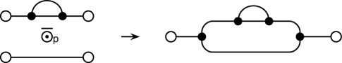
Figure 4.1. The modified parallel operation $\overline{\odot}_{p}$.

Similarly, our modified operation $\overline{\odot}_{s}$ merges the second terminal of the first graph with the first terminal of the second graph, and then smooths away the merged vertex, as illustrated in Figure 4.2.

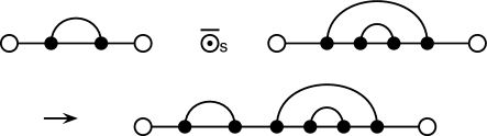
Figure 4.2. The modified parallel operation $\overline{\odot}_{s}$.

The method for calculating the pgd of a dmt-string is given in Section 5.

Step (4). This step concerns the composition of an amalgamation of two double-rooted graphs with univalent roots at one pair of univalent roots, followed by a self-amalgamation at the other two roots. See Section 6 for a description of this computation.

Step (5). This step is the composition of an amalgamation of two double-rooted graphs with univalent roots at one pair of univalent roots, followed by a self-amalgamation at the other two roots. See Section 6 for a description of this computation.

5. PGD of DMT-Strings

Four parallel productions and four series productions will be sufficient to calculate the values of the partials of any dmt-string. The following two sets of four productions each are sufficient to calculate all the partials of a dmt-string. The parallel productions are derived with the aid of Figures 5.1, 5.2, and 5.3. The series productions are self-evident. The genus of each resultant embedding is calculated from its Euler characteristic.

(5.1) $$\qquad uu_{i}^{\bullet}\,\overline{\odot}_{p}\,uu_{j}^{\bullet} \longrightarrow 4uu_{i+j+1}^{\bullet}\quad\hbox{(Figure \ref{fig:uu*uu})}$$

(5.2) $$uu_{i}^{\bullet}\,\overline{\odot}_{p}\,uu_{j}^{\prime} \longrightarrow 4uu_{i+j+1}^{\prime}\quad\hbox{(Figure \ref{fig:uu*uu'})}$$

(5.3) $$uu_{i}^{\prime}\,\overline{\odot}_{p}\,uu_{j}^{\bullet} \longrightarrow 4uu_{i+j+1}^{\prime}\quad\hbox{(mirror of Figure \ref{fig:uu*uu'})}$$

(5.4) $$uu_{i}^{\prime}\,\overline{\odot}_{p}\,uu_{j}^{\prime} \longrightarrow 2uu_{i+j}^{\bullet}+2uu_{i+j}^{\prime}\quad\hbox{(Figure \ref{fig:uu'*uu'})}$$

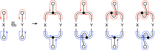
Figure 5.1. Production: $uu_{i}^{\bullet}\,\overline{\odot}_{p}\,uu_{j}^{\bullet}\longrightarrow 4uu_{i+j+1}^{\bullet}$.

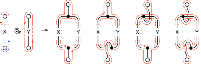
Figure 5.2. Production: $uu_{i}^{\bullet}\,\overline{\odot}_{p}\,uu_{j}^{\prime}\longrightarrow 4uu_{i+j+1}^{\prime}$.

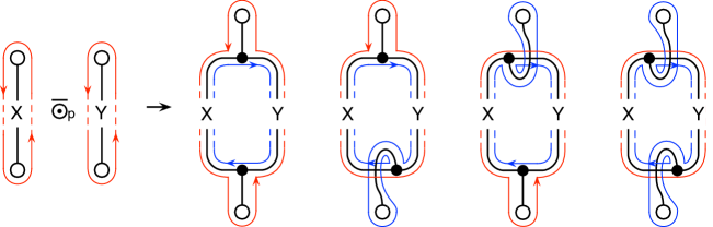
Figure 5.3. Production: $uu_{i}^{\prime}\,\overline{\odot}_{p}\,uu_{j}^{\prime}\longrightarrow 2uu_{i+j}^{\prime}+2uu_{i+j}^{\bullet}$.

(5.5) $$uu_{i}^{\bullet}\,\overline{\odot}_{s}\,uu_{j}^{\bullet} \longrightarrow uu_{i+j}^{\bullet}$$

(5.6) $$uu_{i}^{\bullet}\,\overline{\odot}_{s}\,uu_{j}^{\prime} \longrightarrow uu_{i+j}^{\bullet}$$

(5.7) $$uu_{i}^{\prime}\,\overline{\odot}_{s}\,uu_{j}^{\bullet} \longrightarrow uu_{i+j}^{\bullet}$$

(5.8) $$uu_{i}^{\prime}\,\overline{\odot}_{s}\,uu_{j}^{\prime} \longrightarrow uu_{i+j}^{\prime}$$

Examples

Our first example is the dmt-string $\hat{D}_{2}$ of Figure 5.4, which is of fundamental use in our further calculations. Here we use $\operatorname{pgd}$ (which stands for partitioned genus distribution) as a function.

Figure 5.4. The dmt-string $\hat{D}_{2}$.

We observe that $\hat{D}_{2}$ is representable as $K_{2}\,\overline{\odot}_{p}\,K_{2}$. Therefore,

$$\operatorname{pgd}(\hat{D}_{2}) = \operatorname{pgd}(K_{2}\,\overline{\odot}_{p}\,K_{2})$$

$$= uu_{0}^{\prime}\,\overline{\odot}_{p}\,uu_{0}^{\prime}$$

(5.9) $$\operatorname{pgd}(\hat{D}_{2}) = 2uu_{0}^{\bullet}+2uu_{0}^{\prime}\qquad\hbox{by Prod.\,\eqref{prod:uu'*uu'}}$$

We now apply Eq. (5.4) and the productions above to calculate the partials of the three dmt-strings of the graph of Figure 5.5.

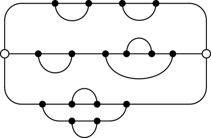
Figure 5.5. A cubic series-parallel graph.

The top dmt-string $N^{1}$ is representable as $\hat{D}_{2}\,\overline{\odot}_{s}\,\hat{D}_{2}$. Therefore,

$$\operatorname{pgd}(N^{1}) = \operatorname{pgd}(\hat{D}_{2}\,\overline{\odot}_{s}\,\hat{D}_{2})$$

$$= (2uu_{0}^{\bullet}+2uu_{0}^{\prime})\,\overline{\odot}_{s}\,(2uu_{0}^{\bullet}+2uu_{0}^{\prime})$$

$$= 2uu_{0}^{\bullet}\,\overline{\odot}_{s}\,2uu_{0}^{\bullet}+2uu_{0}^{\bullet}\,\overline{\odot}_{s}\,2uu_{0}^{\prime}$$

$$\quad\qquad+\;2uu_{0}^{\prime}\,\overline{\odot}_{s}\,2uu_{0}^{\bullet}+2uu_{0}^{\prime}\,\overline{\odot}_{s}\,2uu_{0}^{\prime}$$

$$= 4uu_{0}^{\bullet}+4uu_{0}^{\bullet}+\;4uu_{0}^{\bullet}+4uu_{0}^{\prime}$$

by Prods. (5.5), (5.6), (5.7), (5.8)

(5.10) $$\operatorname{pgd}(N^{1}) = 12uu_{0}^{\bullet}+4uu_{0}^{\prime}$$

The dmt-string $N^{2}$ is representable as $\hat{D}_{2}\,\overline{\odot}_{s}\,(\hat{D}_{2}\,\overline{\odot}_{p}\,K_{2})$. Therefore,

$$\qquad\operatorname{pgd}(N^{2}) = \operatorname{pgd}(\hat{D}_{2}\,\overline{\odot}_{s}\,(\hat{D}_{2}\,\overline{\odot}_{p}\,K_{2}))$$

$$= (2uu_{0}^{\bullet}+2uu_{0}^{\prime})\,\overline{\odot}_{s}\,((2uu_{0}^{\bullet}+2uu_{0}^{\prime})\,\overline{\odot}_{p}\,uu_{0}^{\prime})$$

$$= (2uu_{0}^{\bullet}+2uu_{0}^{\prime})\,\overline{\odot}_{s}\,(8uu_{1}^{\prime}+4uu_{0}^{\bullet}+4uu_{0}^{\prime})$$

by Prods. (5.2), (5.4)

$$= 16uu_{1}^{\bullet}+8uu_{0}^{\bullet}+8uu_{0}^{\bullet}+16uu_{1}^{\prime}+8uu_{0}^{\bullet}+8uu_{0}^{\prime}$$

by Prods. (5.1), (5.2), (5.3), (5.4)

(5.11) $$\operatorname{pgd}(N^{2}) = 24uu_{0}^{\bullet}+8uu_{0}^{\prime}+16uu_{1}^{\bullet}+16uu_{1}^{\prime}$$

The dmt-string $N^{3}$ is representable as $\hat{D}_{2}\,\overline{\odot}_{p}\,\hat{D}_{2}$. Therefore,

$$\operatorname{pgd}(N^{3}) = \operatorname{pgd}(\hat{D}_{2}\,\overline{\odot}_{p}\,\hat{D}_{2})$$

$$= (2uu_{0}^{\bullet}+2uu_{0}^{\prime})\,\overline{\odot}_{p}\,(2uu_{0}^{\bullet}+2uu_{0}^{\prime})$$

$$= 16uu_{1}^{\bullet}+16uu_{1}^{\prime}+16uu_{1}^{\prime}+8uu_{0}^{\bullet}+8uu_{0}^{\prime}$$

by Prods. (5.1), (5.2), (5.3), (5.4)

(5.12) $$\operatorname{pgd}(N^{3}) = 8uu_{0}^{\bullet}+8uu_{0}^{\prime}+16uu_{1}^{\bullet}+32uu_{1}^{\prime}$$

6. Amalgamating DMT-Strings

A parallel operation on two dmt-strings yields a series-parallel graph whose source and target roots are both 2-valent. Figure 6.1 illustrates the productions used to transform the partials of the two antecedent dmt-strings into the partials of the consequent series-parallel graph. We define two partials for the case where $p$ and $q$ are both bivalent and a single walk is twice incident at each:

$$ss_{i}^{\bullet}(G,p,q) = \text{the number of embeddings }G\to S_{i}\text{ such that}$$

$$\hbox{the fb-walks twice incident at $p$ and $q$ are different};$$

$$ss_{i}^{\prime}(G,p,q) = G\to S_{i}$$ the number of embeddings such that

$$\hbox{the same fb-walk is twice incident at $p$ and $q$}.$$

$$dd_{i}^{\prime\prime}(G,p,q) = G\to S_{i}$$ the number of embeddings such that

$$\hbox{the same two fb-walks are twice incident at $p$ and $q$}.$$

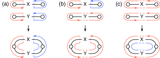
Figure 6.1. Parallel operations on two dmt-strings.

(6.1) $$uu_{i}^{\bullet}\odot_{p}uu_{j}^{\bullet} \longrightarrow ss_{i+j+1}^{\bullet}\qquad\hbox{(Figure \ref{fig:uu*uu->dd}(a))}$$

(6.2) $$uu_{i}^{\bullet}\odot_{p}uu_{j}^{\prime} \longrightarrow ss_{i+j+1}^{\prime}\qquad\hbox{(Figure \ref{fig:uu*uu->dd}(b))}$$

(6.3) $$uu_{i}^{\prime}\odot_{p}uu_{j}^{\bullet} \longrightarrow ss_{i+j+1}^{\prime}\qquad\hbox{(use Figure \ref{fig:uu*uu->dd}(b))}$$

(6.4) $$uu_{i}^{\prime}\odot_{p}uu_{j}^{\prime} \longrightarrow dd_{i+j}^{\prime\prime}\quad\qquad\hbox{(Figure \ref{fig:uu*uu->dd}(c))}$$

Once again, the genus of each resultant embedding is calculated from its Euler characteristic. Continuing with our example of the graph from Figure 5.5, these productions enable us, in turn, to calculate $\operatorname{pgd}(N^{1}\odot_{p}N^{2})$.

$$\qquad\operatorname{pgd}(N^{1}\odot_{p}N^{2}) \!\!=\!\! (12uu_{0}^{\bullet}+4uu_{0}^{\prime})$$

$$\quad\odot_{p}(24uu_{0}^{\bullet}+8uu_{0}^{\prime}+16uu_{1}^{\bullet}+16uu_{1}^{\prime})$$

$$\!\!=\!\! 12uu_{0}^{\bullet}\odot_{p}(24uu_{0}^{\bullet}+8uu_{0}^{\prime}+16uu_{1}^{\bullet}+16uu_{1}^{\prime})$$

$$\quad+~{}4uu_{0}^{\prime}\odot_{p}(24uu_{0}^{\bullet}+8uu_{0}^{\prime}+16uu_{1}^{\bullet}+16uu_{1}^{\prime})$$

$$\!\!=\!\! 288ss_{1}^{\bullet}+96ss_{1}^{\prime}+192ss_{2}^{\bullet}+192ss_{2}^{\prime}$$

$$\quad+96ss_{1}^{\prime}+32dd_{0}^{\prime\prime}+64ss_{2}^{\prime}+64dd_{1}^{\prime\prime}$$

$$\;\;\operatorname{pgd}(N^{1}\odot_{p}N^{2}) \!\!=\!\! 32dd_{0}^{\prime\prime}+64dd_{1}^{\prime\prime}+288ss_{1}^{\bullet}+192ss_{2}^{\bullet}$$

$$\quad+192ss_{1}^{\prime}+256ss_{2}^{\prime}$$

The following six productions will enable us to complete our calculation of the genus distribution of the graph of Figure 5.5, starting from the pgd (6) for $N^{1}\odot_{p}N^{2}$ and the pgd (5.12) for $N^{3}$. We observe that the result of applying these productions is a genus distribution, rather than a partitioned genus distribution. Accordingly, the consequents are of the form $g_{i}$ rather than subscripted partials, thereby indicating only that the resulting embedding surface is $S_{i}$.

(6.6) $$dd_{i}^{\prime\prime}\odot_{p}uu_{j}^{\bullet} \longrightarrow 4g_{i+j+1}\qquad\qquad\hbox{(Figure \ref{fig:dd''0uu})}$$

(6.7) $$dd_{i}^{\prime\prime}\odot_{p}uu_{j}^{\prime} \longrightarrow 2g_{i+j}+2g_{i+j+1}\quad\hbox{(Figure \ref{fig:dd''0uu'})}$$

(6.8) $$ss_{i}^{\bullet}\odot_{p}uu_{j}^{\bullet} \longrightarrow 4g_{i+j+1}\qquad\qquad\hbox{(Figure \ref{fig:ss0uu})}$$

(6.9) $$ss_{i}^{\bullet}\odot_{p}uu_{j}^{\prime} \longrightarrow 4g_{i+j+1}\qquad\qquad\hbox{(Figure \ref{fig:ss0uu'})}$$

(6.10) $$ss_{i}^{\prime}\!\odot_{p}uu_{j}^{\bullet} \longrightarrow 4g_{i+j+1}\qquad\qquad\hbox{(Figure \ref{fig:ss'0uu})}$$

(6.11) $$ss_{i}^{\prime}\!\odot_{p}uu_{j}^{\prime} \longrightarrow 4g_{i+j}\quad\qquad\qquad\hbox{(Figure \ref{fig:ss'0uu'})}$$

Figures 6.6, 6.6, 6.6, 6.6, 6.6, and 6.7 illustrate the six productions (6.6), (6.7), (6.8), (6.9), (6.10), and (6.11), respectively, that collectively provide an algebraic representation of the parallel operation.

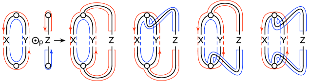
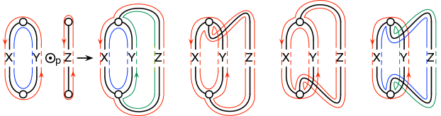
Figure 6.2. $dd_{i}^{\prime\prime}\odot_{p}uu_{j}^{\bullet}\longrightarrow 4g_{i+j+1}$.

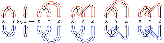
Figure 6.3. $dd_{i}^{\prime\prime}\odot_{p}uu_{j}^{\prime}\longrightarrow 2g_{i+j}+2g_{i+j+1}$.

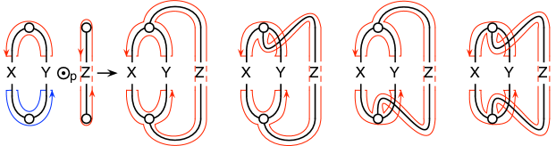
Figure 6.4. $ss_{i}^{\bullet}\odot_{p}uu_{j}^{\bullet}\longrightarrow 4g_{i+j+1}$.

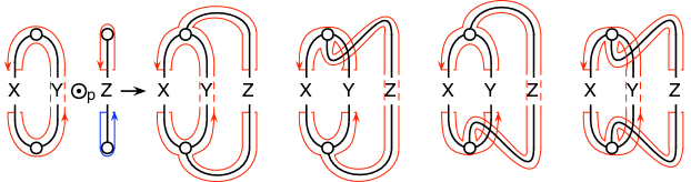
Figure 6.5. $ss_{i}^{\bullet}\odot_{p}uu_{j}^{\prime}\longrightarrow 4g_{i+j+1}$.

Figure 6.6. $ss_{i}^{\prime}\odot_{p}uu_{j}\longrightarrow 4g_{i+j+1}$.

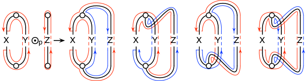
Figure 6.7. $ss_{i}^{\prime}\odot_{p}uu_{j}^{\prime}\longrightarrow 4g_{i+j}$.

$$\operatorname{pgd}(N^{1}\odot_{p}N^{2}) \!=\! 32dd_{0}^{\prime\prime}+64dd_{1}^{\prime\prime}+288ss_{1}^{\bullet}+192ss_{2}^{\bullet}+192ss_{1}^{\prime}+256ss_{2}^{\prime}$$

$$\operatorname{pgd}(N^{3}) = 8uu_{0}^{\bullet}+8uu_{0}^{\prime}+16uu_{1}^{\bullet}+32uu_{1}^{\prime}$$

$$32dd_{0}^{\prime\prime}\odot_{p}8uu_{0}^{\bullet} = 1024g_{1}$$

$$32dd_{0}^{\prime\prime}\odot_{p}8uu_{0}^{\prime} = 512g_{0}+512g_{1}$$

$$32dd_{0}^{\prime\prime}\odot_{p}16uu_{1}^{\bullet} = 2048g_{2}$$

$$32dd_{0}^{\prime\prime}\odot_{p}32uu_{1}^{\prime} = 2048g_{1}+2048g_{2}$$

$$64dd_{1}^{\prime\prime}\odot_{p}8uu_{0}^{\bullet} = 2048g_{2}$$

$$64dd_{1}^{\prime\prime}\odot_{p}8uu_{0}^{\prime} = 1024g_{1}+1024g_{2}$$

$$64dd_{1}^{\prime\prime}\odot_{p}16uu_{1}^{\bullet} = 4096g_{3}$$

$$64dd_{1}^{\prime\prime}\odot_{p}32uu_{1}^{\prime} = 4096g_{2}+4096g_{3}$$

$$288ss_{1}^{\bullet}\odot_{p}8uu_{0}^{\bullet} = 9216g_{2}$$

$$288ss_{1}^{\bullet}\odot_{p}8uu_{0}^{\prime} = 9216g_{2}$$

$$288ss_{1}^{\bullet}\odot_{p}16uu_{1}^{\bullet} = 18432g_{3}$$

$$288ss_{1}^{\bullet}\odot_{p}32uu_{1}^{\prime} = 36864g_{3}$$

$$192ss_{2}^{\bullet}\odot_{p}8uu_{0}^{\bullet} = 6144g_{3}$$

$$192ss_{2}^{\bullet}\odot_{p}8uu_{0}^{\prime} = 6144g_{3}$$

$$192ss_{2}^{\bullet}\odot_{p}16uu_{1}^{\bullet} = 12288g_{4}$$

$$192ss_{2}^{\bullet}\odot_{p}32uu_{1}^{\prime} = 24576g_{4}$$

$$192ss_{1}^{\prime}\odot_{p}8uu_{0}^{\bullet} = 6144g_{2}$$

$$192ss_{1}^{\prime}\odot_{p}8uu_{0}^{\prime} = 6144g_{1}$$

$$192ss_{1}^{\prime}\odot_{p}16uu_{1}^{\bullet} = 12288g_{3}$$

$$192ss_{1}^{\prime}\odot_{p}32uu_{1}^{\prime} = 24576g_{2}$$

$$256ss_{2}^{\prime}\odot_{p}8uu_{0}^{\bullet} = 8192g_{3}$$

$$256ss_{2}^{\prime}\odot_{p}8uu_{0}^{\prime} = 8192g_{2}$$

$$256ss_{2}^{\prime}\odot_{p}16uu_{1}^{\bullet} = 16384g_{4}$$

$$256ss_{2}^{\prime}\odot_{p}32uu_{1}^{\prime} = 32768g_{3}$$

By summation of the right-hand sides of the equations above, we obtain the genus distribution

$$\begin{array}[]{c|rrrrr}{\rm genus}&0\hfil&1\hfil&2\hfil&3\hfil&4\hfil\\ \hline\cr{\rm\#embeddings}&512&10752&68608&129024&53248\end{array}$$

This calculation has been confirmed by a computer program based on the Heffter-Edmonds algorithm.

Theorem 6.1.

The time required by Algorithm 4.1 is at most quadratic in the number of vertices of the graph $G$ supplied as input.

Proof.

Choosing an edge and its endpoints $s$ and $t$, as required by Step (1), takes constant time. The time needed for Step (2), which is achieved by partitioning the edge-set of the given graph $G$ into the edge-sets of the three dmt-strings, is linear in the number of vertices of $G$, using depth-first search.

When two subgraphs are amalgamated during Step (3), the contribution to the partials of the merged graph corresponding to a pair of nonzero-valued subscripted partials, one in the pgd of the first amalgamand and the other in the pgd of the second amalgamand, is calculated by the application of one of the Productions (5.1), …, (5.8). Since the number of nonzero-valued subscripted partials for any graph is linear in the number of vertices, the time to calculate the pgd of the merged graph is proportional to the product of the numbers of vertices in the two amalgamands. Suppose that the numbers of vertices of the fragments of an dmt-string are $x_{1},x_{2},\ldots,x_{p}$. Since the vertices in two different fragments will be merged into a combined fragment only once during the reassembly of the dmt-string, the number of applications of productions during the entire reassembly is at most

$$\sum_{i\neq j}x_{i}x_{j}$$

However,

$$\sum_{i\neq j}x_{i}x_{j}~{}<~{}(x_{1}+x_{2}+\cdots+x_{p})^{2}$$

from which we infer that the total time is at most quadratic in the number of vertices of the dmt-string.

To see that Step (4) can be done in quadratic time, first observe that the number of nonzero partials in $\operatorname{pgd}(N^{1})$ and $\operatorname{pgd}(N^{2})$ is linear in the maximum genus of $N^{1}$ and $N^{2}$, since partials can be nonzero only for genera with genus less than or equal to maximum genus and for every genus in this range there is only a constant number of different types of partials. Furthermore, it is well known that the maximum genus of any graph $G$ is bounded from above by $\beta(G)$ (see [GrTu87]), the cycle rank of $G$, which in turn is linear in the number of vertices for any graph with maximum degree $3$. Accordingly, there is only a linear number of nonzero partials for both $N^{1}$ and $N^{2}$, yielding at most a quadratic number of combinations needed to calculate $\operatorname{pgd}(N^{1}\odot_{p}N^{2})$. Finally, each combination of two partials can be computed in constant time using appropriate choices from Productions (5.1), …, (5.4), which implies that Step (4) can indeed be done in quadratic time in the number of vertices.

The argument that Step (5) uses only quadratic time is similar to that for Step (4) — the number of nonzero partials is again linear in the number of vertices; and each computation, this time involving one of the Productions (6.6), …, (6.11), can be done in constant time. ∎

7. Extending to All Graphs of Treewidth $\leq 2$ and Maximum Degree $\leq 3$

The bar-amalgamation of two disjoint rooted graphs $(G,u)$ and $(H,v)$ is the result of running a new edge (the “bar”) between $u$ and $v$.

Proposition 7.1.

The genus distribution of the bar-amalgamation of graphs $(G,u)$ and $(H,v)$ is the constant multiple of the convolution of the genus distributions of $G$ and $H$. The constant factor is the product of the degree of $u$ in $G$ and the degree of $v$ in $H$.

Proof.

This is Theorem 5 of [GrFu87]. ∎

To extend Algorithm 4.1 to any graph $G$ of treewidth at most 2 and maximum degree 3, we infer from Proposition 2.1 that each biconnected component of $G$ either is isomorphic to $K_{2}$ or is a homeomorphic copy of a 3-regular biconnected graph. Moreover, each of the latter kind of biconnected components meets only the $K_{2}$-type components. Thus, the graph $G$ is an iterated bar-amalgamation of biconnected series-parallel graphs. Accordingly, to calculate its genus distribution, we calculate the genus distributions of its biconnected components, take corresponding convolutions, and multiply by scalars corresponding to degrees of vertices at the ends of the bars.

8. Conclusions

Starting with a quadratic-time algorithm for calculating the genus distribution of all cubic biconnected series-parallel graphs, we have constructed a quadratic-time algorithm for the genus distribution of any graph of treewidth at most 2 and maximum degree at most 3. The advantage of this case-specific algorithm over the more general algorithm of [Gr14] is the ease with the case-specific algorithm can be used to obtain numerical results for specific graphs.

References

- [BWGT09] L. W. Beineke, R. J. Wilson, J. L. Gross, and T. W. Tucker, Editors, Topics in Topological Graph Theory, Cambridge Univ. Press, 2009.
- [Bo98] H. L. Bodlaender, A partial -arboretum of graphs with bounded treewidth, Theoretical Comp. Sci. 209 (1998), 1–45.
- [BPT09] R. B. Borie, R. G. Parker, and C. A. Tovey, Solving problems on recursively constructed graphs, ACM Compu. Surveys 41 (2009), 1–51.
- [Die06] R. Diestel, Graph Theory, Third Edition, Springer, 2006.
- [Dir52] G. A. Dirac, A property of 4-chromatic graphs and some remarks on critical graphs, J. London Math. Soc. 27 (1952), 85–92.
- [Du65] R. J. Duffin, Topology of series-parallel networks, J. Math. Analysis and Applications 10 (1965), 303–318.
- [Ep92] D. Eppstein, Parallel recognition of series-parallel graphs, Information and Computation 98 (1992), 41–55.
- [Gr10] J. L. Gross, Genus distribution of graphs under surgery: adding edges and splitting vertices, New York J. Mathematics 16 (2010), 161–178.
- [Gr11a] J. L. Gross, Genus distribution of graph amalgamations: Self-pasting at root-vertices, Australasian J. Combin. 49 (2011), 19–38.
- [Gr11b] J. L. Gross, Genus distributions of cubic outerplanar graphs, J. of Graph Algorithms and Applications 15 (2011), 295–316.
- [Gr13] J. L. Gross, Embeddings of cubic Halin graphs: genus distributions, Ars Math. Contemporanea 6 (2013), 37–56.
- [Gr14] J. L. Gross, Embeddings of graphs of fixed treewidth and bounded degree, Ars Math. Contemporanea 7 (2014), 379–403.
- [GrFu87] J. L. Gross and M. Furst, Hierarchy for imbedding-distribution invariants of a graph, J. Graph Theory 11 (1987), 205–220.
- [GKP10] J. L. Gross, I. F. Khan, and M. I. Poshni, Genus distribution of graph amalgamations: Pasting at root-vertices, Ars Combin. 94 (2010), 33–53.
- [GrTu87] J. L. Gross and T. W. Tucker, Topological Graph Theory, Dover, 2001; (original edn. Wiley, 1987).
- [KMR09] K. Kawarabayashi, B. Mohar, and B. Reed, A simpler linear time algorithm for embedding graphs into an arbitrary surface and the genus of graphs of bounded tree-width, Proc. 49th Ann. Symp. on Foundations of Computer Science (FOCS’08) IEEE (2008), 771–780.
- [KPG10] I. F. Khan, M. I. Poshni, and J. L. Gross, Genus distribution of graph amalgamations at roots of higher degree, Ars Math. Contemporanea 3 (2010), 121–138.
- [KPG12] I. F. Khan, M. I. Poshni, and J. L. Gross, Genus distribution of , Discrete Math. 312 (2012), 2863–2871.
- [MoTh01] B. Mohar and C. Thomassen, Graphs on Surfaces, Johns Hopkins University Press, 2001.
- [PKG10] M. I. Poshni, I. F. Khan, and J. L. Gross, Genus distribution of edge-amalgamations, Ars Math. Contemporanea 3 (2010), 69–86.
- [PKG11] M. I. Poshni, I. F. Khan, and J. L. Gross, Genus distribution of 4-regular outerplanar graphs, Electronic J. Combin. 18 (2011) #P212, 25pp.
- [PKG12] M. I. Poshni, I. F. Khan, and J. L. Gross, Genus distribution of graphs under self-edge-amalgamations, Ars Math. Contemporanea 5 (2012), 127–148.
- [Th89] C. Thomassen, The graph genus problem is NP-complete, J. Algorithms 10 (1989), 568–576.