Nonlinear dynamical models from time series

Abstract

We present an optimization process to estimate parameters in systems of ordinary differential equations from chaotic time series. The optimization technique is based on a variational approach, and numerical studies on noisy time series demonstrate that it is very robust and appropriate to reduce the complexity of the model. The proposed process also allows to discard the parameters with scanty influence on the dynamic.

I Introduction

The question if given a time series measurements we can identify an underlying dynamical model and predict its future values begin certainly with Yule Yule (1929) and is posed today in several disciplines as well as economy, geophysics or fluids dynamics. In economy research, the short time prediction plays an important role in financial risk decision; notwithstanding dynamical models for the different observable are not known. Then the huge quantities of data we dispose do possible statistical approaches. Antagonist examples are seismic inversion, and oil and water research where the model is in general well known, i.e. the wave equation or Darcy like models, but experimental data are only accessible at the frontier of the studied region. As a consequence geophysics research has developed powerful tools of collecting the bulk information. An other interesting and different example is fluid dynamics because it has a good model, the Navier Stokes equation, and the possibility of taking data everywhere. Unfortunately the harvests of the initial conditions are difficult since requires the measurements of these functions over a three-dimensional domain. Then typical experiences in hydrodynamics produce time series and so, the most practical situations deal with time series. All these examples are different outlooks of the same universal question: How can we obtain dynamical systems from measurements? It is awful question because we have an infinite number of models M belonging to a specific class of functions (radial functions, polynomials, etc.) which must be specified in view of the a priori knowledge about the problem, and even when the model is known it will be parameterized by a set of unknown numbers $\alpha$.

In this paper we consider a classical problem in nonlinear dynamical systems: given a noisy time series, we want to capture the underlying dynamics and, to do that we suppose that it can be modeled by a coupled system of ordinary differential equations (ODE) parameterized by a set of numbers $\alpha$. We propose a constraint minimization to reduce the model complexity, that is, to find out parameters with scanty influence on the dynamic ($\alpha_{j}\sim 0$), and in addition to reduce the overfitting risk. The order of the model is given by the number of non zero components of the vector $\alpha$. We apply a variational approach to compute the derivatives of $\alpha_{j}$ for a defined measure ${\cal F}$ and a step descent method to find the optimal set of parameters. We will show on chaotic time series that this technique is robust and able to reconstruct orbits from noisy data.

II Identification Method

The baseline time series are generated by the following model of $m$ coupled ODE :

$$\frac{dA_{i}(t)}{dt}-f_{i}(\alpha,A_{1}(t),\cdots,A_{m}(t))=0\ \ \ \ \ \ \ i=1,\cdots,m$$ (1)

where the parameter vector $\alpha\in R^{n}$. The integration method is an Euler schema with time step $\delta t=0.01$ to assure the stability for long time integrations. A Gaussian noise with zero average and standard deviation $\tau$, ${\cal N}(0,\tau)$, is then added to the noiseless signal $A(t)$ to build the “observed” data $D(t)$. Different noisy time series are produced by modifying the standard deviation $\tau$. The amount of noise over the signal is quantified by the signal-to-noise ratio (SNR)

$$SNR=\left({S_{data}\over S_{noise}}\right)^{2}$$

where $S$ stands by the root mean square, in particular in our case $S_{noise}=\tau$. The logarithm relation $10\log_{10}SNR$ gives the ratio in $dB$. The “observed” data used for computations are

$$D_{i}(t)=A_{i}(t)+{\cal N}(0,\tau)\ \ i=1,\cdots,m$$ (2)

where we assumed the measurements performed at fixed sampling time $T<\delta t$.

To asses the quality of the reconstruction we define a functional ${\cal F}=\sum_{1}^{m}{\cal F}_{i}$ which consists on the addition of the Euclidean distances between the observed $D_{i}$ and the reconstructed data $M_{i}$ on $w$ time windows over a time integration $L$ :

$${\cal F}_{i}=\sum_{w}\int^{L}_{0}||\ D_{i}(t)-M_{i}(t)\ ||^{2}\ \delta(T)\ dt.$$

The reconstructed data $M_{i}$ are generated by a model $M(\alpha)$ at fixed parameters $\alpha$, and we note that for a free noise series, when $M(t)$ and $D(t)$ coincide both with $A(t)$ we have ${\cal F}=0$. According to the fact that the measurement are performed in a discrete way we define a delta function $\delta(T)$ related to the sampling time $T$; for instance $\delta(T)=1$ for multiple of the sampling time of observed data and zero elsewhere.

We are in presence of an inverse problem, that is to seek for an optimal set of parameters of a model with respect to a measure ${\cal F}(\alpha)$. The classical approach for a $n$ dimensional problem is the unconstrained optimization: minimize ${\cal F}(\alpha)$ with $\alpha\in R^{n}$. This becomes most of the time a classical least squares approach or one of its several variations. For a linear model in the parameters $\alpha$, the cost function is quadratic and there is only one global minimum. We can estimate directly the derivatives of the model $M$ from observed data $D_{i}(t)$ but noise prevent an appropriate evaluation. We recall that inverse problems are generally ill-conditioned which is reflected in the lack of robustness face to noise showed in numerical simulations Fullana et al. (1997); Timmer et al. (2000).

This work presents a constrained optimization and we solve it using a variational approach. The formal definition of constrained optimization is the following: minimize ${\cal F}(\alpha)$ with $\alpha\in R^{n}$ subject to a constraints $g(\alpha)=0$. We define specifically the $g(\alpha)$ as the proposed model $M$ for the “observed” data. We therefore write $g(\alpha)=0$ as

$$\frac{dM_{i}}{dt}-f_{i}(\alpha,M_{1},\cdots,M_{m})=0\ \ \ \ \ \ \ i=1,\cdots,m$$ (3)

where $m$ is the dimension of the data series and the fonction $f_{i}(\alpha,M_{1},\cdots,M_{m})$ belonging to some specific class of functions. Explicit dependency in time is removed for sake of readability. On each windows $w$ the model is integrated between $0$ and $L$ and the initial conditions are the “observed” values at the beginning, $M_{i}(0)=D_{i}(0)$. Within this situation we are close to an initial value problem in the framework of the multiple shooting approach.

We define the following Lagrangian function

$${\cal L}_{i}={\cal F}_{i}+\sum_{w}\int^{L}\left(dM_{i}/dt-f_{i}(\alpha,M)\right)V_{i}\ dt$$ (4)

where $V=V(\alpha,M,V)$ is the dual variable corresponding to the constraint or Lagrange multiplier. As the constraint is always verified we have ${\cal L}_{i}={\cal F}_{i}$ for any choice of $V_{i}$. The total variation is then

$$\delta{\cal L}_{i}=\delta_{\alpha}{\cal L}_{i}\delta\alpha+\delta_{V}{\cal L}_{i}\delta V_{i}+\delta_{M}{\cal L}_{i}\delta M.$$ (5)

We observe that the term $\delta_{V}{\cal L}_{i}=0$ is equivalent to the imposed constraints and therefore zero. Provided that $\delta_{V}{\cal L}_{i}=0$ it is clear that we can computed the gradient explicitly as a matter of fact ${\cal L}_{i}={\cal F}_{i}$ implies

$${\delta{\cal L}_{i}\over\delta\alpha}={\delta{\cal F}_{i}\over\delta\alpha}.$$ (6)

Imposing $\delta_{M}{\cal L}_{i}=0$ results in a system for $V$ that must be integrated backward in time over the length window $L$. For each window $w$ this leads to the following expression

$$-\frac{dV_{i}}{dt}=\delta_{M}f(\alpha,M,V)+2e_{i}(t)\delta(T)$$ (7)

with the boundary condition set at the final time $L$, $V_{i}(L)=0$ and where $e_{i}(t)=D_{i}(t)-M_{i}(t)$ is the local error.

The gradient of the components $i$ of the cost function, ${\cal F}_{i}$, can be write explicitly as

$$\delta_{\alpha}{\cal F}_{i}=-\sum_{w}\int^{L}\delta_{\alpha}f_{i}\cdot\ V_{i}\ dt.$$ (8)

and finally the gradient for a given parameter $\alpha_{j}$ is

$$\delta_{\alpha_{j}}{\cal F}=\sum_{i}\delta_{\alpha_{j}}{\cal F}_{i}$$

Once the gradient established we perform a descent in the direction of the gradient of ${\cal F}$. We apply a quasi-Newton method which uses the function gradient at each iteration Gill et al. (1981).

The optimisation algorithm find an optimal set which depends on the noise level $\tau$ and on the window length $L$, $\bar{\alpha}=\bar{\alpha}(\tau,L)$. The model is evaluated on each window for fixed parameters $\alpha$ for different $L$ starting from $L=1$. The $w$ windows of temporal length $L$ are thus equivalent to the fitting intervals of the multiple shooting method but the difference being that we do not impose the matching between solutions at the interval frontier ($t=T$). This exemple has been well examined in reference Baake et al. (1992) in two cases : when the model is available and when we specify only its class.

Figure 1: Scheme for the optimisation process for $L=1,2,3$ (from the top to the bottom).

The Figure 1 shows a schematic illustration of the process for $L=1,2,3$. We paid attention to a specific data (the third one beginning from the left), we observe that it is used on the window : (i) for $L=1$ as initial condition, (ii) for $L=2$ as the final condition, and (iii) for $L=3$ as internal data. Then, it is straightforward of concluding that data are used more that once in the process in contrast to the multiple shooting method, and that “window overlap” enhances the statistics. To improve yet the statistic we repeat the procedure over a large number of probes $np$ of length $wL$. Using the optimal values from each probe we compute the average value ${\bar{\alpha}}$ and the standard deviation $\sigma=\sqrt{\sum_{k=1}^{np}({\bar{\alpha}}-\alpha^{opt}_{k})^{2}}$. We can apply this procedure to experimental data by splitting experimental data series in probes of size $wL$.

The Figure 2 shows the variation of three parameters ${\bar{\alpha}}$ as function of the window length $L$ for the Lorenz equation with noise equal to 14.53 $dB$ $(\tau=1.5)$. In this case we have $np=10^{3}$ and the probe size $wL$ is set to $10^{3}$. We will discuss the Lorenz model and the figure in the next section. The standard deviation $\sigma$ is represented by horizontal ticks. Note that the average values converge from $L=25-30$, in term of optimisation we can infer that no more information is available.

Finally parameters $\alpha$ with small mean values and weak ratio ${{\bar{\alpha}}\over\sigma}$ are discarded and this determines the end of the first stage of the optimisation process. The ratio ${{\bar{\alpha}}\over\sigma}$ is called reliability which is an estimation of the statistical reliability (the difference is that we known the average value ${\bar{\alpha}}$ instead of the actual value). A central point is how do we quantify it. We decide that $\alpha_{opt}<eps$ are discarded and we set $eps=0.02$ which is quite arbitrary. We argue that if the parameters $\alpha$ are of the order of 1 this $eps$ implies that the discarded parameters are at least around 2% of the keeping ones. On the contrary in a case with parameters $\alpha$ of the order of less than 1 we have to re-define this cutoff. Next, for the reliability the criterion is less arbitrary as long as parameters with $\log_{10}({{\bar{\alpha}}\over\sigma})<0$ are considered weak, the cutoff is then ${\bar{\alpha}}\sim\sigma$.

We keep parameters which in general, have high reliability, small $\sigma$, and are different from zero. We reduce by the procedure the number of parameters to avoid overfitting. In the following stages we use the original model with a smaller number of parameters and the recursive procedure stops when the number of parameters does not change anymore. In practice three or four stages are suffisant to finish the optimisation procedure.

III Applications and Discusion

The strategy of model construction and parameter selection presented above is applied on a particular class of functions, a full 2d-order polynomial taking into account the squares and the cross products for $m=3$ :

$$dM_{1}(t)/dt= \alpha_{1}M_{1}(t)+\alpha_{2}M_{2}(t)+\alpha_{3}M_{3}(t)+\alpha_{4}M_{1}(t)M_{2}(t)+\alpha_{5}M_{1}(t)M_{3}(t)+$$

$$\alpha_{6}M_{2}(t)M_{3}(t)+\alpha_{7}M_{1}^{2}(t)+\alpha_{8}M_{2}^{2}(t)+\alpha_{9}M_{3}^{2}(t)$$

$$dM_{2}(t)/dt= \alpha_{10}M_{1}(t)+\alpha_{11}M_{2}(t)+\alpha_{12}M_{3}(t)+\alpha_{13}M_{1}(t)M_{2}(t)+\alpha_{14}M_{1}(t)M_{3}(t)+$$

$$\alpha_{15}M_{2}(t)M_{3}(t)+\alpha_{16}M_{1}^{2}(t)+\alpha_{17}M_{2}^{2}(t)+\alpha_{18}M_{3}^{2}(t)$$

$$dM_{3}(t)/dt= \alpha_{19}M_{1}(t)+\alpha_{20}M_{2}(t)+\alpha_{21}M_{3}(t)+\alpha_{22}M_{1}(t)M_{2}(t)+\alpha_{23}M_{1}(t)M_{3}(t)+$$

$$\alpha_{24}M_{2}(t)M_{3}(t)+\alpha_{25}M_{1}^{2}(t)+\alpha_{26}M_{2}^{2}(t)+\alpha_{27}M_{3}^{2}(t).$$

The vector of parameters $\alpha$ is composed of 27 values. The integration method is an Euler schema with time step $\delta t=0.01$ and the sampling time $T=0.1$. For statistics we use $np=10^{3}$ and the probe size $wL$ is set to $10^{3}$. We use the same model ($M=A$) to generate the noisy series. We note that the chaotic Lorenz model Lorenz (1963) and the Roessler model Rössler (1976) belong to this class.

We apply therefore the optimisation process to both models. Chaotic data series from the Lorenz model are built using equation (III) with the following seven non-zero $\alpha$ components : $\alpha_{1}=-10.,\alpha_{2}=10.,\alpha_{10}=28.,\alpha_{11}=-1.,\alpha_{14}=-1.,\alpha_{21}=-2.666,\alpha_{22}=1.$. In order of obtaining the “observed” data we add some amount of noise (equation (2)) and we pick data at sampling times.

The set of optimal parameters will indeed depend on the noise level $\tau$ and on the window length $L$ and, in addition, the functional ${\cal F}$ will become more and more non linear as long as $L$ growths Henning et al. (2004). With this in mind we monitor the $\bar{\alpha}$ as a function of the window length $L$ starting from $L=1$. The case $L=1$ is particular, because in a strict sense the numerical evaluation of the derivatives of the model (III), $dM_{1}(t)/dt$ by the way, are almost the same using either $\delta t$ or $T$. It easily follows that for $\delta t=T$ and $L=1$ the optimisation problem becomes a classical least square, then the functional function ${\cal F}$ is quadratic and the solution unique and moreover we can compute the derivatives explicitly from ${\cal F}$ without doing a variational approach.

The optimal parameters of window length $L=1$ are used as initial guess for the window length $L=2$ and we continue until convergence with the window size $L$. The key features of the process are showed in Figure 2 for three parameters $\alpha_{1},\alpha_{2},\alpha_{3}$ where the standard deviation $\sigma$ is represented by horizontal ticks.

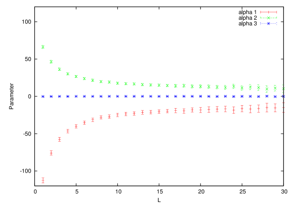
Figure 2: Optimal $\alpha$ as function of the length window $L$ for a Lorenz model with noise level around of 14.53 $db$.

The level of noise is high, $\tau=1.5$ in equation (2), which is around of 14.53 $dB$. Note that the average values converge from $L=25-30$. Pay attention to the $y$ axis scale, the parameter $\alpha_{3}$ is not but fluctues around zero, its reliability is low and it is discarded at the first stage as is shown in Figure 3.

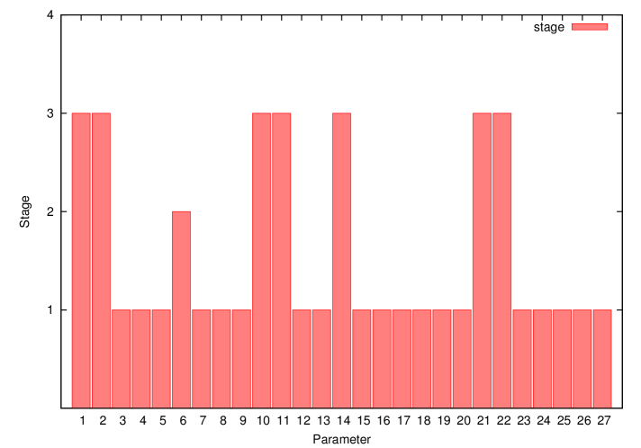
Figure 3: Stages of the optimization process for each parameter $\alpha_{i}$, $i=1\dots 27$ of the model. Same case than Figure 2 . See text for details.

The Figure 3 presents then the process of discarding parameters : the $y$ axis say if given parameter is dropped off or not a that stage. In some detail we can see that parameter 1 ($\alpha_{1}$) is stilll present at the end of the process (stage 3), and conversely parameter 3 ($\alpha_{3}$) disappear in the first run (stage 1). As noted earlier parameters $\alpha$ with small mean values and weak reliability are discarded. In the Figure 4 we show the equivalent of Figure 2 but at the end of the process (stage 3).

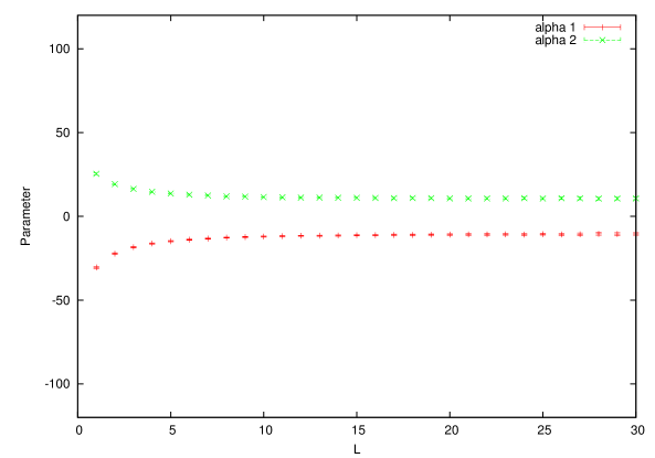
Figure 4: Same than Figure 2. Note that $\alpha_{3}$ has been discarded at the stage 1.

We note that the convergence is done before $L=25-30$ and both the optimal parameters and dispersions are less affected by noise (in particular compare optimal values for small window length $L$ in Figure 2).

The Table 1 shows optimal values and standard deviation for several noisy series ($\tau=0.5,1.0,1.5,2.0,2.5$).

$\alpha$	$\tau=0.5(10^{2})$	$\tau=0.5(10^{3})$	$\tau=1.0(10^{3})$	$\tau=1.5(10^{3})$	$\tau=2.0(10^{3})$	$\tau=2.5(10^{3})$
1	-10.359 $\pm$ 0.221	-10.374 $\pm$ 0.247	-10.578 $\pm$ 0.314	-10.664 $\pm$ 0.404	-10.673 $\pm$ -0.509	-10.591 $\pm$ 2.801
2	9.955 $\pm$ 0.180	9.956 $\pm$ 0.202	9.995 $\pm$ 0.248	10.042 $\pm$ 0.291	10.149 $\pm$ 0.378	10.084 $\pm$ 3.658
10	28.673 $\pm$ 0.572	28.706 $\pm$ 0.549	29.127 $\pm$ 0.779	29.297 $\pm$ 0.984	29.332 $\pm$ 1.202	29.601 $\pm$ 5.653
11	-0.954 $\pm$ 0.075	0.952 $\pm$ 0.078	-0.968 $\pm$ 0.110	-0.991 $\pm$ 0.147	-1.028 $\pm$ 0.312	-0.168 $\pm$ 4.504
14	-1.021 $\pm$ 0.019	-1.022 $\pm$ 0.018	-1.034 $\pm$ 0.027	-1.041 $\pm$ 0.036	-1.043 $\pm$ 0.051	-1.042 $\pm$ 0.162
21	-2.608 $\pm$ 0.020	-2.607 $\pm$ 0.022	-2.603 $\pm$ 0.033	-2.598 $\pm$ 0.043	-2.589 $\pm$ 0.062	-2.495 $\pm$ 0.474
22	1.023 $\pm$ 0.021	1.023 $\pm$ 0.023	1.036 $\pm$ 0.035	1.051 $\pm$ 0.048	1.047 $\pm$ 0.078	1.167 $\pm$ 1.120
26	–	–	–	–	0.054 $\pm$ 0.085	0.094 $\pm$ 0.457

Table 1: Optimal parameters for the Lorenz model, average values and standard deviation. (columns two and three) Noise level is $\tau=0.5$ for $np=10^{2}$ and $np=10^{3}$. (columns four to seven) Noise leves are $\tau=1.0,1.5,2.0,2.5$ ($18.06,14.53,12.04,10.10$ in $dB$ using the baseline signal of $A_{1}$) for $np=10^{3}$ probes.

Each column shows the average value $\bar{\alpha}$ and its standard deviation. Columns two and three illustrate their behavior for the same noise level $\tau=0.5$ and for two probes number $np=10^{2}$ and $np=10^{3}$, we can see that statistic does not change too much, we conserve for that reason $np=10^{3}$ for the subsequent computations. Columns four to seven present the evolution of the numerical findings for noise levels $\tau=1.0,1.5,2.0,2.5$ which is in $dB$ $18.06,14.53,12.04,10.1$ using the noiseless signal $A_{1}$. At $\tau=2.0$ the parameter 26 ($\alpha_{26})$ does not disappear and is still present at the end of the optimization process. We note that the other parameter are not affected by its presence and the numerical reconstruction (not shown) using the ODE system (equation (III)) does not differs from the original time series.

On the contrary, the next result ($\tau=2.5$) shows that parameter 11 is seriously affected varying of one order of magnitude, from $\sim-1$ to $\sim-0.1$. Parameters coming from the linearized system as $dM_{2}(t)/dt\sim\alpha_{11}M_{2}(t)$ among others are really difficult to obtain. These terms give, in a first approximation exponential solutions behaving like $M_{2}(t)\sim e^{\alpha_{11}t}$. When noise is added we shadow the orbits and a lot of them are equivalent, we are in the conditions of the “shadowing” lemma (Farmer and Sidorovitch (1991) and references therein) but for an inverse problem : under these conditions there are not enough information to provide accurate estimates of the parameter values and then the optimization algorithm is not able to separate contributions coming from linear or nonlinear terms Smith et al. (2010). Even though the parameters are affected by noise the reconstruction using equation (III) shows the typical “strange” Lorenz attractor and we can see in Figure 5 that the time series for the variable $M_{2}(t)$ is very similar to the original $A_{2}(t)$. Nevertheless a close examination of the “burst” regions show us that the reconstructed one is less sharp. This characteristic is governed by the coefficient $\alpha_{11}$ which, as mentioned above, is not well evaluated.

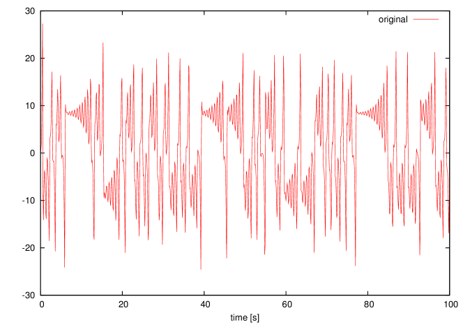
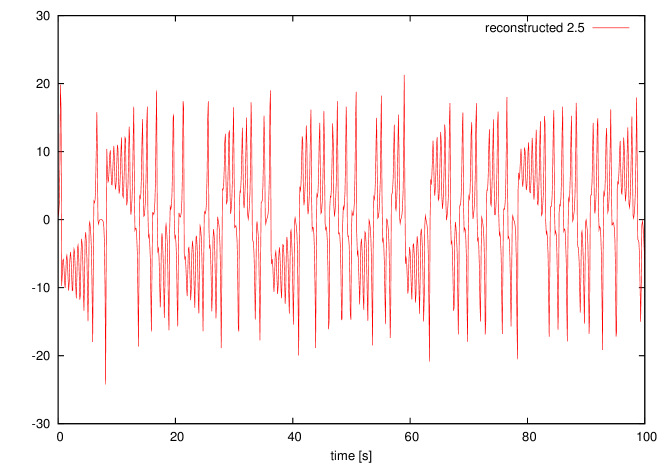
Figure 5: Lorenz model : (top) original temporal series $A_{2}(t)$ and (bottom ) reconstructed one $M_{2}(t)$ for $\tau=2.5$.

Coming back to column 5 ($\tau=2.0$) and examining the parameter 26 ($\alpha_{26}$) we remark that even if it is larger than the cutoff value ”eps” its standard deviation is also quite large, then its reliability is poor. Figure 6 presents the logarithm of the reliability of all parameters, this result sugests that satisfying both criteria (small mean values and weak ratio ${{\bar{\alpha}}\over\sigma}$) conjointly is too restrictive. We restart the process using either small mean values OR weak ratio ${{\bar{\alpha}}\over\sigma}$, the “OR” condition for the rest of the paper.

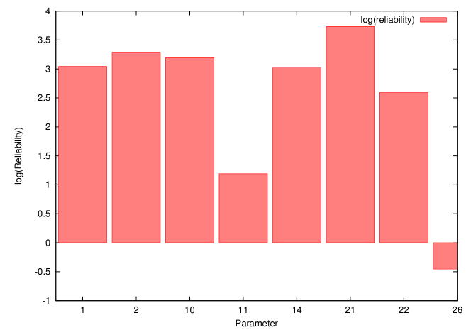
Figure 6: Logarithm of the reliability for coefficients of Table 1, column 6.

The Table 2 shows numerical results for $\tau=2.0$ and $\tau=2.5$ for the “OR” condition, in both cases the optimal values are closed to the actual ones and their resist quite well to the noise, except for the parameter 11 which is becoming not reliable, ${{\bar{\alpha}_{11}}\over\sigma_{11}}\sim 1$.

$\alpha$	$\tau=2.0,np=10^{3}$	$\tau=2.5,np=10^{3}$
1	-10.712 $\pm$ -0.639	-10.724 $\pm$ -0.868
2	10.067 $\pm$ 0.426	10.124 $\pm$ 0.747
10	29.492 $\pm$ 1.629	29.699 $\pm$ 2.630
11	-1.021 $\pm$ -0.351	-1.124 $\pm$ -1.021
14	-1.052 $\pm$ -0.061	-1.066 $\pm$ -0.098
21	-2.590 $\pm$ -0.125	-2.566 $\pm$ -0.224
22	1.069 $\pm$ 0.074	1.105 $\pm$ 0.167

Table 2: Optimal coefficients for the Lorenz model using the “OR” condition (see text). Noise values are $\tau=2.0$ and $\tau=2.5$.

We apply now the “OR” condition to the Rossler model Rössler (1976) . Observed data for the Rossler model are generated by equations (III) with parameter $\alpha=\{\alpha_{2}=-1.0,\alpha_{3}=-1.0,\alpha_{10}=1.0,\alpha_{11}=0.38,\alpha_{19}=0.3,\alpha_{21}=-4.5,\alpha_{23}=1.0\}$ plus a noise value as mentioned above. Noise levels are $\tau=0.2,0.4,0.8,1.0$ or in $dB$, $23.72,17.70,11.68,9.74$ using the noiseless signal $A_{1}$.

$\alpha$	$\tau=0.2,np=10^{3}$	$\tau=0.4,np=10^{3}$	$\tau=0.8,np=10^{3}$	$\tau=1.0,np=10^{3}$
2	-1.000 $\pm$ 0.005	-0.993 $\pm$ 0.012	-1.002 $\pm$ 0.016	-1.003 $\pm$ 0.015
3	-0.998 $\pm$ 0.005	-0.994 $\pm$ 0.010	-0.983 $\pm$ 0.020	-0.987 $\pm$ 0.022
10	0.998 $\pm$ 0.006	0.995 $\pm$ 0.013	0.979 $\pm$ 0.022	0.979 $\pm$ 0.027
11	0.375 $\pm$ 0.004	0.365 $\pm$ 0.008	0.328 $\pm$ 0.033	0.329 $\pm$ 0.054
19	0.313 $\pm$ 0.006	0.412 $\pm$ 0.034	0.442 $\pm$ 0.087	0.433 $\pm$ 0.141
21	-4.476 $\pm$ 0.040	-4.476 $\pm$ 0.077	-4.296 $\pm$ 0.168	-4.329 $\pm$ 0.215
23	0.992 $\pm$ 0.010	0.974 $\pm$ 0.018	0.920 $\pm$ 0.055	0.927 $\pm$ 0.081

Table 3: Optimal coefficients for the Rossler model using the “OR” condition (see text). Noise values are $\tau=0.2,0.4,0.8,1.0$ ($23.72,17.70,11.68,9.74$ in $dB$).

We use the model (III) to identify the unknown parameters and we look the behavior of the optimal parameters $\alpha$. Table 3 shows the numerical findings, the first point is that the procedure is able to determine the important model’s parameters even in presence of high amount of noise. Second, that the standard deviations increase linearly with the noise level. Third, that the optimal values resist quite well to noise excepted parameter 19 $\alpha_{19}$ which has around $30\%$ of error. This parameter corresponds to the term $dM_{3}(t)/dt\sim\alpha_{13}M_{1}(t)$ (see the model (III)) and is directly responsible for the aperiodic and rough burst in coordinate 3 on the Rossler model. This burst dynamics is not easy of capturing because very sharp and short (typical half time peak is around of 1 sec, which is $L=10$).

Numerical optimisations show that the optimal values are in excellent accord and the reconstructed orbits (not shown) are in agreement with the original ones.

IV Conclusion

We have presented an optimization procedure able to retain the important parameters for a mathematical model given a noisy time series. We have applied the procedure to two chaotic series from the Lorenz and the Rossler models. We have demonstrated using an ODE system that the procedure (i) is appropriate to reduce the complexity of the model, (ii) is powerful to make a parameters estimation, and (iii) is very robust against noise. We also observe that we can reduce the time integration, and in the limit $\delta t\rightarrow 0$ we could compute the continuos parameters of a system.

In our numerical examples we know the actual number and value of the model parameters, this is an important help to decide what criterium we have to use. We have shown that using both criteria, small mean values and weak ratio ${{\bar{\alpha}}\over\sigma}$, conjointly is too constrain. When at least one criterium is fulfilled we have proved that the optimization procedure is improved. In a case of unknown data series we have to ameliorate the procedure, an interesting way could be to compute the covariance matrix $({\partial^{2}F\over\partial^{2}{\alpha}})^{-1}$ and analyse the eigenvalues to display linear combinations.

We can yet improve the procedure working on the initial conditions for each window : the choice $M_{i}(0)=D_{i}(0)$ is may be not the optimal, numerical tests show that using $M_{i}(0)=A_{i}(0)$ (which is in fact impossible on real data) the optimal results are closest to the actual values. Then an issue could be either to make a some kind of average process in the neighbor of the initial conditions or add some constraints as well as in the multiple shooting approach. We could define the initial conditions $M_{i}(0)$ as parameters to optimize as in reference Fullana and Zaleski (1997) but the number of unknowns will become too important, adding by the way $m\ w$ parameters ($w$ being the window number) to the optimization problem.

However many questions are still open : the application to real data or the tractability for applying this procedure to systems including unobserved data series (when data dimension is greater that model dimension). The present procedure should be effective for different problems from classical or less classical parameter identification Timmer et al. (2000); Vyasarayani et al. (2012) to control/synchronization applications Yu and Parlitz (2008); Peng et al. (2011). In particular an extension to high degree polynomial class is straightforward and could be effortless applied to neuronal or electrical circuits Schumann-Bischoff and Parlitz (2011).

References

- Yule (1929) G. U. Yule, Philos. Trans. Roy. Soc. London A 226, 267 (1929).
- Fullana et al. (1997) J. M. Fullana, P. Le Gal, M. Rossi, and S. Zaleski, Physica D 102, 37 (1997).
- Timmer et al. (2000) J. Timmer, H. Rust, W. Horbelt, and H. Voss, Physics Letters A 274, 123 (2000).
- Gill et al. (1981) P. E. Gill, W. Murray, and M. H. Wright, Practical Optimization (Academic Press, 1981).
- Baake et al. (1992) E. Baake, M. Baake, H. Bock, K. Briggs, et al., Physical Review A 45, 5524 (1992).
- Lorenz (1963) E. N. Lorenz, J. Atmos. Sci. 20, 130 (1963).
- Rössler (1976) O. E. Rössler, Physics Letters A 57, 397 (1976).
- Henning et al. (2004) U. Henning, J. Timmer, and J. Kurths, International Journal of Bifurcation and Chaos 14, 1905 (2004).
- Farmer and Sidorovitch (1991) J. D. Farmer and J. J. Sidorovitch, Physica D 47, 373 (1991).
- Smith et al. (2010) L. A. Smith, M. C. Cuellar, H. Du, and K. Judd, Physics Letters A 374, 2618 (2010), ISSN 0375-9601, URL http://www.sciencedirect.com/science/article/pii/S0375960110004561.
- Fullana and Zaleski (1997) J.-M. Fullana and S. Zaleski, Physical Review Letters 27 (1997).
- Vyasarayani et al. (2012) C. P. Vyasarayani, T. Uchida, and J. McPhee, Phys. Rev. E 85, 036201 (2012), URL http://link.aps.org/doi/10.1103/PhysRevE.85.036201.
- Yu and Parlitz (2008) D. Yu and U. Parlitz, Phys. Rev. E 77, 066221 (2008), URL http://link.aps.org/doi/10.1103/PhysRevE.77.066221.
- Peng et al. (2011) H. Peng, L. Li, Y. Yang, and F. Sun, Phys. Rev. E 83, 036202 (2011), URL http://link.aps.org/doi/10.1103/PhysRevE.83.036202.
- Schumann-Bischoff and Parlitz (2011) J. Schumann-Bischoff and U. Parlitz, Phys. Rev. E 84, 056214 (2011), URL http://link.aps.org/doi/10.1103/PhysRevE.84.056214.