Feedback, scatter and structure in the core of the PKS 0745–191 galaxy cluster

Abstract

We present Chandra X-ray Observatory observations of the core of the galaxy cluster PKS 0745–191. Its centre shows X-ray cavities caused by AGN feedback and cold fronts with an associated spiral structure. The cavity energetics imply they are powerful enough to compensate for cooling. Despite the evidence for AGN feedback, the Chandra and XMM-RGS X-ray spectra are consistent with a few hundred solar masses per year cooling out of the X-ray phase, sufficient to power the emission line nebula. The coolest X-ray emitting gas and brightest nebula emission is offset by around 5 kpc from the radio and X-ray nucleus. Although the cluster has a regular appearance, its core shows density, temperature and pressure deviations over the inner 100 kpc, likely associated with the cold fronts. After correcting for ellipticity and projection effects, we estimate density fluctuations of $\sim 4$ per cent, while temperature, pressure and entropy have variations of $10-12$ per cent. We describe a new code, mbproj, able to accurately obtain thermodynamical cluster profiles, under the assumptions of hydrostatic equilibrium and spherical symmetry. The forward-fitting code compares model to observed profiles using Markov Chain Monte Carlo and is applicable to surveys, operating on 1000 or fewer counts. In PKS0745 a very low gravitational acceleration is preferred within 40 kpc radius from the core, indicating a lack of hydrostatic equilibrium, deviations from spherical symmetry or non-thermal sources of pressure.

1 Introduction

The radiative cooling time of the dominant baryonic component, the intracluster medium (ICM), in the centres of many clusters of galaxies is much shorter than the age of the cluster. In the absence of any heating, a cooling flow should form (Fabian, 1994) where the material should rapidly cool out of the X-ray band at 10s to 100s solar masses per year. Mechanical feedback by AGN in cluster cores can energetically provide the balancing source of heat (McNamara & Nulsen, 2012), although the tight balance suggests that the heating is gentle and close to continuous (Fabian, 2012).

An ideal place to study the mechanisms of feedback and the effect of the AGN on the surrounding cluster is in the most extreme objects. PKS 0745–191 is the radio source located at the centre of a rich galaxy cluster at a redshift of 0.1028. The cluster has been well studied by X-ray observatories since the launch of Einstein (Fabian et al., 1985). The galaxy cluster is relaxed and has a steeply-peaked surface brightness profile. It is the X-ray brightest at $z>0.1$ (Edge et al., 1990), with a 2 to 10 keV X-ray luminosity of $1.6\times 10^{45}\hbox{$\rm\thinspace erg\rm\thinspace s^{-1}\,$}$ and is the nearest cluster with a mass deposition rate inferred from the X-ray surface brightness profile of greater than $1000\hbox{$\hbox{$\rm\thinspace M_{\odot}$}\rm\thinspace yr^{-1}\,$}$ (Allen et al., 1996).

The central galaxy is undergoing considerable star formation. Optical spectra suggest $\sim 50\hbox{$\hbox{$\rm\thinspace M_{\odot}$}\rm\thinspace yr^{-1}\,$}$ of star formation (Johnstone, Fabian & Nulsen, 1987) and infrared observations using Spitzer give its total IR luminosity as $3.8\times 10^{44}\hbox{$\rm\thinspace erg\rm\thinspace s^{-1}\,$}$, which corresponds to a star formation rate of $17\hbox{$\hbox{$\rm\thinspace M_{\odot}$}\rm\thinspace yr^{-1}\,$}$ (O’Dea et al., 2008). In addition, the cluster is a strong emitter in H$\alpha$ (L[H$\alpha$+Nii] = $2.8\times 10^{42}\hbox{$\rm\thinspace erg\rm\thinspace s^{-1}\,$}$; Heckman et al. 1989), in an extended filamentary nebula, the luminosity of which is on the extreme end of the distribution of values observed in clusters (Crawford et al., 1999). Salomé & Combes (2003) have also detected CO(1-0) and CO(2-1) emission lines in PKS0745, implying an H₂ mass of $4\times 10^{9}\hbox{$\rm\thinspace M_{\odot}$}$. Hicks & Mushotzky (2005) found a UV excess from the central galaxy of $\sim 12\times 10^{43}\hbox{$\rm\thinspace erg\rm\thinspace s^{-1}\,$}$. This is clearly an interesting object where heating is not matching cooling.

The very unusual and interesting radio source in PKS0745 was studied in detail by Baum & O’Dea (1991). The radio jets appear to have been disrupted on small scales so that the large scale structure is amorphous. This is seen in just a few other radio galaxies in dense environments (e.g. 3C317 in A2052, Zhao et al. 1993; and PKS 1246–410 in the Centaurus cluster, Taylor, Fabian & Allen 2002).

PKS0745 is one of the nearest galaxy clusters to exhibit strong gravitational lensing (Allen, Fabian & Kneib, 1996). The 0-th order image of a Chandra HETGS observation of the cluster was examined by Hicks et al. (2002), finding a central temperature of $4-5\rm\thinspace keV$. The properties of the ICM in PKS0745 have been measured to beyond the virial radius (George et al., 2009) using Suzaku, showing a considerable flattening of the entropy profile. Walker et al. (2012) have improved on this analysis with the aid of further observations to better understand the X-ray background contribution. They find that at radii beyond $1.9\rm\thinspace Mpc$ the cluster is not in hydrostatic equilibrium or there is significant non-thermal pressure support.

At the redshift of the cluster, 1 arcsec on the sky corresponds to 1.9 kpc, assuming that $H_{0}=70\hbox{$\hbox{$\rm\thinspace km\rm\thinspace s^{-1}\,$}\rm\thinspace Mpc^{-1}$}$. In this paper, the relative Solar abundances of Anders & Grevesse (1989) were used. North is to the top and east is to the left in images, unless otherwise indicated. The Galactic Hydrogen column density towards PKS0745 is high, around $4.2\times 10^{21}\hbox{$\rm\thinspace cm^{-2}\,$}$, weighting the nearest 0.695 deg pixels in the Leiden/Argentine/Bonn (LAB) survey (Kalberla et al., 2005). However, these pixels show large variation with a standard deviation of $4\times 10^{20}\hbox{$\rm\thinspace cm^{-2}\,$}$.

2 Chandra images

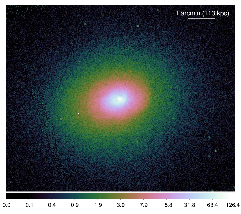
Figure 1: Exposure-corrected and background-subtracted 0.5 to 7 keV image using 0.492 arcsec pixels, smoothed with a Gaussian with $\sigma=1$ pixel. The units are $10^{-8}$ photon $\rm\thinspace s^{-1}\,$$\rm\thinspace cm^{-2}\,$.

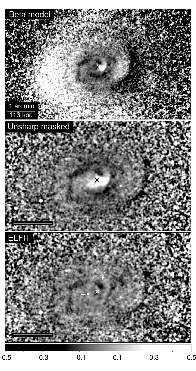
Figure 2: (Top panel) Fractional residuals of $\beta$ model fit to 0.5 to 7 keV exposure-corrected and background-subtracted data. (Centre panel) Unsharp masked image, showing fractional residuals between data smoothed by a Gaussian of $\sigma=2$ and 16 pixels (1 and 8 arcsec). (Bottom panel) Fractional difference between data (smoothed by 2 pixels) and elfit multi-elliptical model. Note that the lower two panels are zoomed in compared to the top panel. The white arrows in the bottom panel show the location of two depressions. ‘$\times$’ marks the location of the central radio source.

We examined two ACIS-S Chandra observations of PKS0745 with observation identifiers of 12881 (exposure time of 118.1 ks) and 2427 (exposure time of 17.9 ks). We did not examine observation 507 which contained extensive flares. We reprocessed the observations to filter background events using VFAINT mode. To remove flares we used an iterative $\sigma$-clipping algorithm on lightcurves from the CCD S1, which is back-illuminated like ACIS S3, in the 2.5 to 7 keV band. No additional flares were seen in a higher energy band. The total cleaned exposure of the observations was 135.5 ks. The total exposure-corrected and background-subtracted image of the cluster is shown in Fig. 1. For the background subtraction we used blank-sky-background event files. Separate backgrounds were used for each observation with the the exposure time in each CCD adjusted so that the count rate in the 9 to 12 keV band matched the respective observation. The background event files were reprojected to match the observations. The background images for each observation and CCD were divided by the ratio of the background to observation exposure times, before subtracting from the observation image. A monochromatic exposure map at 1.5 keV was then used for exposure correction.

Due to the bright central peak, it is difficult to look for structure in the X-ray image. The features are seen more easily by looking at the residuals of a model fit or by using unsharp-masking. The top panel of Fig. 2 shows the residuals from an elliptical $\beta$ model fit to the surface brightness. The centre panel shows a closer view of the central region, but using unsharp masking to remove the larger scale emission. The bottom panel shows the residuals to an elfit model made up by logarithmically interpolating between 20 ellipses fitted to logarithmically spaced contours of surface brightness (Sanders & Fabian, 2012). In all residuals, a spiral morphology can be seen. In addition, there is a sharp drop in surface brightness $\sim 1$ arcmin to the west of the core, some of which is modelled out by the elfit procedure. The centre of the cluster contains two central depressions in surface brightness to the north-west and south-east (see white arrows in bottom panel). The depressions are around 20 per cent fainter than the surrounding material. There are other possible features in the central region, but many of these appear to be related to the swirling spiral feature. The negative spiral residuals are around 10 per cent in magnitude.

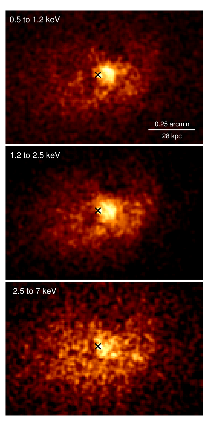
Figure 3: Unsharp-masked images in the different spectral bands. These images have the original image smoothed by a Gaussian with $\sigma=1$ pixel, subtracting 0.5 times the image smoothed by 8 pixels. ‘$\times$’ marks the location of the central radio source.

Fig. 3 shows the centre of the cluster in soft, medium and hard bands. The image shows that there is soft X-ray emission in the rims of the surface brightness depressions. In addition, there is an extended bright region of soft X-ray emission a few arcsec to the west of the central nucleus, seen as a point source. We examine this in more detail in Section 3.

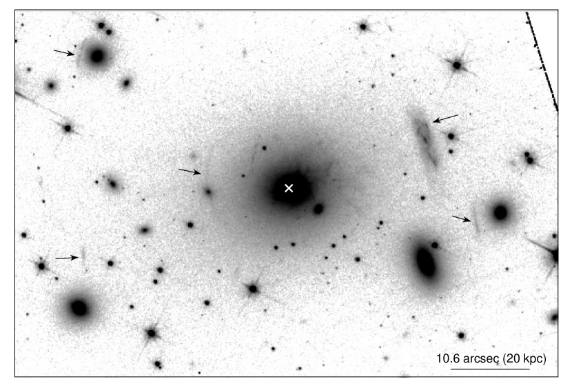
Figure 4: HST F814W image of the centre of the cluster. Positions of possible strong lensing arcs are marked by arrows and ‘$\times$’ shows the central radio source position. The image was created from WFPC2 datasets U59N0101R, U59N0102R and U59N0103R.

3 Nuclear region

The brightest central galaxy (BCG) was observed by HST in 1999 using the WFPC2 instrument with F184W and F55W filters, with exposure times of $3\times 600$ and $3\times 700$ s, respectively. At the redshift of PKS0745, the F814W band contains the H$\alpha$+Nii emission lines. In Fig. 4 we show the F814W image of the centre of the cluster. A number of strong lensing arcs can be seen in the image. We have marked possible arcs with arrows. The strongest arc is 18 arcsec to the west-north-west (WNW) of the core. Another arc 12 arcsec to the east is also clearly seen. Allen, Fabian & Kneib (1996) noted three arcs, which were the strong arc to the WNW, the other south of that, plus another further south. We do not see this final arc, but see three further candidates to the east. An emission line nebula is present in the inner 20 kpc, but is difficult to see against the continuum of the galaxy in this image.

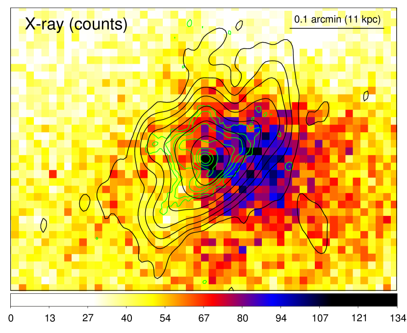
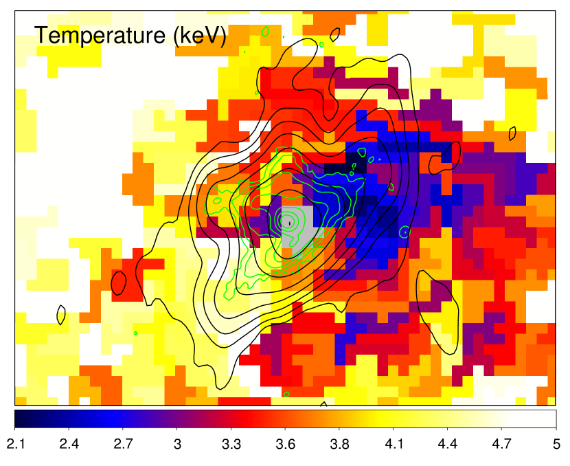
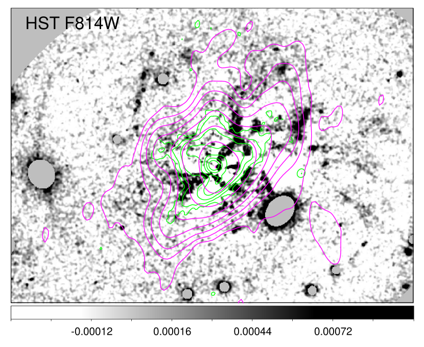
Figure 5: (Top panel) X-ray count image of the nuclear region of the cluster between 0.5 and 7 keV. The smaller contours show 8.4 GHz VLA-detected radio emission (Taylor, Barton & Ge, 1994), logarithmically spaced between $5\times 10^{-5}$ and 0.05 Jy beam^-1. The larger contours show 1.4 GHz emission with 8 contours between 0.0003 and 0.66 Jy beam^-1. (Centre panel) X-ray temperature map in keV from spectral fitting of regions with a signal to noise of 20 ($\sim 400$ counts). (Bottom panel) HST F814W image after subtraction of a smooth model. The grey regions are excluded point sources or galaxies, or lie outside the smooth model.

Figure 6: Powerlaw fit to the spectrum of the nucleus. Assuming Galactic absorption, the photon index of $1.8\pm 0.2$ and its luminosity is $(6.2\pm 1.2)\times 10^{41}\hbox{$\rm\thinspace erg\rm\thinspace s^{-1}\,$}$ between 2 and 10 keV. The spectrum is rebinned for display to have a minimum signal to noise ratio of 3 in each spectral bin.

An X-ray image of the region around the nucleus can be seen in the top panel of Fig. 5. The point source associated with the nucleus is observed to the east of a brighter region of emission. Fig. 6 shows the spectrum of the nucleus extracted from a 1 arcsec radius region, using a background region from 1 to 2.4 arcsec radius. We fit the spectrum between 0.5 and 7 keV, minimising the C-statistic. It can be fit with either a powerlaw or a thermal model. Assuming that there is no additional absorption above Galactic values (using the value of $4.2\times 10^{21}\hbox{$\rm\thinspace cm^{-2}\,$}$; Kalberla et al. 2005), the best fitting temperature is 5.1 keV. The more physical powerlaw model gives a photon index of $1.8\pm 0.2$ and has a 2 to 10 keV luminosity of $(6.2\pm 1.2)\times 10^{41}\hbox{$\rm\thinspace erg\rm\thinspace s^{-1}\,$}$. Hlavacek-Larrondo & Fabian (2011) found a luminosity of $(7.5\pm 3.0)\times 10^{41}\hbox{$\rm\thinspace erg\rm\thinspace s^{-1}\,$}$ by spectral fitting a powerlaw to the previous short Chandra observation, assuming no additional absorption.

As part of this programme we performed observations between 1-2 GHz with the newly upgraded Very Large Array (VLA). The observations lasted for five hours on 21 October 2012 and consisted of 16 spectral windows of 64 MHz each covering the entire 1-2 GHz band. In Fig. 5 we show contours of the 1376 MHz radio emission, derived from a single spectral window. The data were calibrated and imaged in AIPS using standard procedures. Results from a full multi-frequency synthesis using the entire band will be presented in a future paper.

We constructed an X-ray temperature map using regions with a signal to noise ratio of 20 (around 400 counts per bin). The regions were selected using the contour binning algorithm of Sanders (2006), using a maximum ratio between the length and width of the bins of 2, and creating bins by following the surface brightness on a 0.5 to 7 keV image smoothed with a kernel adjusted to have a signal to noise ratio of 15 (225 counts). Spectra were extracted from each of the observations and combined. We created response and ancillary response matrices for each bin, weighting the response regions by the number of counts in the 0.5 to 7 keV band. Background spectra were extracted from standard background event files, reprojected to match the foreground observations. The background event files exposure times were adjusted to match the count rate in the foreground observations in the 9 to 12 keV band. The background spectra for the different observations were added, throwing away photons from the shorter observation background spectra to maintain the ratio of effective exposure time between the observations foregrounds and backgrounds. When spectral fitting, the Galactic absorption was fixed at $4.2\times 10^{21}\hbox{$\rm\thinspace cm^{-2}\,$}$ and the metallicity was frozen at $0.44\hbox{$\thinspace\mathrm{Z}_{\odot}$}$ (an average value of the centre taken from maps created with higher signal to noise per bin). We used the apec thermal spectral model (Smith et al., 2001) with phabs photoelectric absorption (Balucinska-Church & McCammon, 1992), fitting between 0.5 and 7 keV.

It can be seen that the coolest X-ray emitting gas lies a few kpc to the west of the nucleus (Fig. 5 centre panel). The minimum projected temperature drops to around 2.1 keV. The radio source at 1.4 and 8.4 GHz shows a complex morphology. The coolest X-ray emitting material lies close to the the western extension of the radio source, but there is little cool material in other directions. This coolest material does not have a significantly different metallicity from nearby gas ($0.38\pm 0.05\hbox{$\thinspace\mathrm{Z}_{\odot}$}$). If we allow the metallicity to be free when fitting the map spectra, we do not see any regions with anomalously low or high metallicity.

Fig. 4 showed an HST image of the cluster (see Section 2). In Fig. 5 (bottom panel) we reveal the H$\alpha$ emitting filaments by subtracting a smooth model. This was an elfit elliptical model fitted to 20 surface brightness contours, excluding other bright sources. The filaments to the north-west appear to follow the 1.4 GHz contours. This is where the bulk of the emission is concentrated and is coincident with the coolest X-ray emitting gas. However, other filaments (e.g. the radial filaments to the west) are not coincident with currently detected radio emission.

4 Central spectra

Table 1: Best fitting values in spectral fits to the Chandra data extracted from the central 1.0 arcmin region, where the cooling time is less than 7.7 Gyr. The results are for models from one to three thermal components (apec), with photoelectric absorption applied (phabs). We also examine a cooling flow model mkcflow, which assumes the gas is radiatively cooling between two temperatures at a certain mass deposition rate ($\dot{M}$). Shown are the absorbing column densities ($n_{\mathrm{H}}$), temperatures ($T$), metallicities ($Z$) and model normalisations (Norm; measured in xspec normalisation units). In these fits we assumed that each component had the same metallicity. For the cooling flow model, we tied the temperature of the apec component to the upper temperature of the mkcflow model.

Model	Parameter	Value
phabs(apec)	$n_{\mathrm{H}}$ ($10^{22}\hbox{$\rm\thinspace cm^{-2}\,$}$)	$0.372\pm 0.002$
	$Z$ ($Z_{\odot}$)	$0.40\pm 0.01$
	$T$ (keV)	$6.38\pm 0.05$
	Norm ($10^{-4}$)	$377\pm 1$
	$\chi^{2}_{\nu}$	$1.32=579/440$
phabs(apec+apec)	$n_{\mathrm{H}}$ ($10^{22}\hbox{$\rm\thinspace cm^{-2}\,$}$)	$0.398\pm 0.004$
	$Z$ ($Z_{\odot}$)	$0.40\pm 0.01$
	$T_{1}$ (keV)	$6.24\pm 0.05$
	$T_{2}$ (keV)	$0.67\pm 0.04$
	Norm 1 ($10^{-4}$)	$381\pm 2$
	Norm 2 ($10^{-4}$)	$7.7\pm 1.3$
	$\chi^{2}_{\nu}$	$1.19=522/438$
phabs(apec+apec+apec)	$n_{\mathrm{H}}$ ($10^{22}\hbox{$\rm\thinspace cm^{-2}\,$}$)	$0.409\pm 0.004$
	$Z$ ($Z_{\odot}$)	$0.43\pm 0.01$
	$T_{1}$ (keV)	$10.9\pm 0.8$
	$T_{2}$ (keV)	$4.8\pm 0.2$
	$T_{3}$ (keV)	$0.64\pm 0.03$
	Norm 1 ($10^{-4}$)	$140\pm 15$
	Norm 2 ($10^{-4}$)	$246\pm 16$
	Norm 3 ($10^{-4}$)	$9.7\pm 1.2$
	$\chi^{2}_{\nu}$	$1.11=485/436$
phabs(apec+mkcflow)	$n_{\mathrm{H}}$ ($10^{22}\hbox{$\rm\thinspace cm^{-2}\,$}$)	$0.393\pm 0.003$
	$Z$ ($Z_{\odot}$)	$0.40\pm 0.01$
	$T_{\mathrm{high}}$ (keV)	$6.65\pm 0.06$
	$T_{\mathrm{low}}$ (keV)	$0.17\pm 0.03$
	Norm ($10^{-4}$)	$350\pm 5$
	$\dot{M}$ ($M_{\odot}$ yr-1)	$112\pm 20$
	$\chi^{2}_{\nu}$	$1.19=522/438$
phabs($5\times$mkcflow)	$n_{\mathrm{H}}$ ($10^{22}\hbox{$\rm\thinspace cm^{-2}\,$}$)	$0.446\pm 0.005$
	$Z$ ($Z_{\odot}$)	$0.41\pm 0.01$
	$\dot{M}(T)$	See Fig. 7
	$\chi^{2}_{\nu}$	$1.24=540/437$
phabs($9\times$mkcflow)	$n_{\mathrm{H}}$ ($10^{22}\hbox{$\rm\thinspace cm^{-2}\,$}$)	$0.438\pm 0.008$
	$Z$ ($Z_{\odot}$)	$0.43\pm 0.01$
	$\dot{M}(T)$	See Fig. 7
	$\chi^{2}_{\nu}$	$1.10=477/433$

We extracted the Chandra spectrum from within a radius of 1.0 arcmin, where the mean radiative cooling time is less than 7.7 Gyr (see Section 6), the time since $z=1$. We fitted this spectrum between 0.5 and 7 keV by minimising the $\chi^{2}$ statistic in xspec (Arnaud, 1996), after grouping it to have a minimum of 20 counts per spectral bin. Models (listed in Table 1) with 1, 2 and 3 apec thermal components were fitted, assuming that the components have the same metallicity and are absorbed by the same phabs Galactic photoelectric absorption. We also fitted the spectrum with a model with a single thermal component plus a cooling flow model (Fabian, 1994), which assumes that the plasma is radiatively cooling from an upper temperature to a lower temperature at a certain rate in $\hbox{$\rm\thinspace M_{\odot}$}\rm\thinspace yr^{-1}\,$. In this model, we use the same temperature for the thermal component as the upper temperature of the cooling flow model and allow the lower temperature to be free. All of these models give similar values for the metallicity ($\sim 0.4\hbox{$\thinspace\mathrm{Z}_{\odot}$}$) and the absorbing column density ($\sim 0.4\times 10^{22}\hbox{$\rm\thinspace cm^{-2}\,$}$).

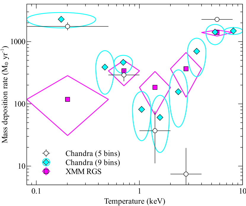
Figure 7: Central temperature distribution, parametrised as the rate of mass deposition as a function of temperature. The results are for the Chandra spectrum from the inner arcmin radius and the XMM-RGS spectra. For Chandra we used models with 5 (circles) and 9 (diamonds) temperature bins and for XMM we used 5 bins (squares). The parameter values and uncertainties were obtained with an MCMC analysis.

The models support a wide range in temperature within the examined region. We can examine the temperature distribution in more detail by fitting the data with multiple cooling flow models in consecutive sets of temperature intervals. This model parametrises the distribution of gas temperature in terms of the rate of matter which would need to be radiatively cooling in particular temperature bands to give rise to the spectrum observed. If all matter was radiatively cooling, this would give a constant value as a function of temperature. Fig. 7 shows the distribution obtained with either 5 or 9 different ranges in temperature. In these fits, each component was assumed to have the same metallicity and was absorbed by the same column density (shown in Table 1). The error bars were obtained from the output chain of a Markov Chain Monte Carlo (MCMC) analysis of the spectral fit, using emcee (Foreman-Mackey et al., 2012) with 200 walkers and a 2000 iterations after a burn period of 500 iterations. emcee uses the affine invariant MCMC sampler of Goodman & Weare (2010). The average acceptance fraction was 43 per cent and the mean autocorrelation time in the chain was 24 iterations, indicating that our results had converged.

Table 2: Spectral fitting results for XMM RGS data. For details on the values shown, see Table 1.

Model	Parameter	Value
phabs(apec+apec)	$n_{\mathrm{H}}$ ($10^{22}\hbox{$\rm\thinspace cm^{-2}\,$}$)	$0.40\pm 0.02$
	$Z$ ($Z_{\odot}$)	0.40 (fixed)
	$T_{1}$ (keV)	$4.4_{-0.4}^{+0.5}$
	$T_{2}$ (keV)	$0.84\pm 0.08$
	Norm 1 ($10^{-4}$)	$290\pm 9$
	Norm 2 ($10^{-4}$)	$11\pm 4$
	C-stat	$4504$
phabs(apec+mkcflow)	$n_{\mathrm{H}}$ ($10^{22}\hbox{$\rm\thinspace cm^{-2}\,$}$)	$0.39\pm 0.02$
	$Z$ ($Z_{\odot}$)	0.40 (fixed)
	$T_{\mathrm{high}}$ (keV)	$5.9_{-0.8}^{+1.2}$
	$T_{\mathrm{low}}$ (keV)	$0.49_{-0.19}^{+0.14}$
	Norm ($10^{-4}$)	$220\pm 26$
	$\dot{M}$ ($M_{\odot}$ yr-1)	$267_{-85}^{+94}$
	C-stat	$4505$
phabs($5\times$mkcflow)	$n_{\mathrm{H}}$ ($10^{22}\hbox{$\rm\thinspace cm^{-2}\,$}$)	$0.40\pm 0.02$
	$Z$ ($Z_{\odot}$)	0.40 (fixed)
	$\dot{M}(T)$	See Fig. 7
	C-stat	$4509$

The cluster was also observed by XMM-Newton for 28.3 ks using its RGS instruments in observation 0105870101. We extracted spectra using a cross-dispersion range containing 90 per cent of the PSF width (equivalent to a strip approximately 50 arcsec wide across the cluster) and 90 per cent of the pulse-height distribution. Spectra were extracted in wavelength space. After removing flares using a cut of 0.2 counts per second on CCD 9, with flag values of 8 or 16 and an absolute cross-dispersion angle of less than $1.5\times 10^{-4}$, we obtained an exposure time of 21.6 ks. We used a background region using the spatial region beyond 98 per cent of the cross-dispersion PSF. Data for the two detectors were merged using rgscombine.

The spectra were jointly fit, minimising the C-statistic in xspec. We fit the first order spectrum between $7$ and $20$Å and the second order spectrum between $7$ and $17$Å. Due to the relatively poor quality of the spectra, we fixed the metallicity when fitting to $0.40\hbox{$\thinspace\mathrm{Z}_{\odot}$}$, the value obtained in the Chandra analyses. We show the results for our spectral fitting, using some of the models used for the Chandra spectral fitting, in Table 2.

A two-component thermal model obtains a lower temperature component at $\sim 0.8$ keV, as found from fitting the Chandra spectra. The spectra appear consistent with around $270\hbox{$\hbox{$\rm\thinspace M_{\odot}$}\rm\thinspace yr^{-1}\,$}$ of cooling from 6 to 0.5 keV temperature. This value is larger than that obtained from Chandra, but if the $\dot{M}$ as a function of temperature is examined (Fig. 7), the XMM and Chandra values are consistent over much of that range, except at the lowest temperatures, where results from CCD spectra are unlikely to be accurate. It is likely that the different overall value is due to the different temperature sensitivities of the two instruments.

5 Central spectral maps

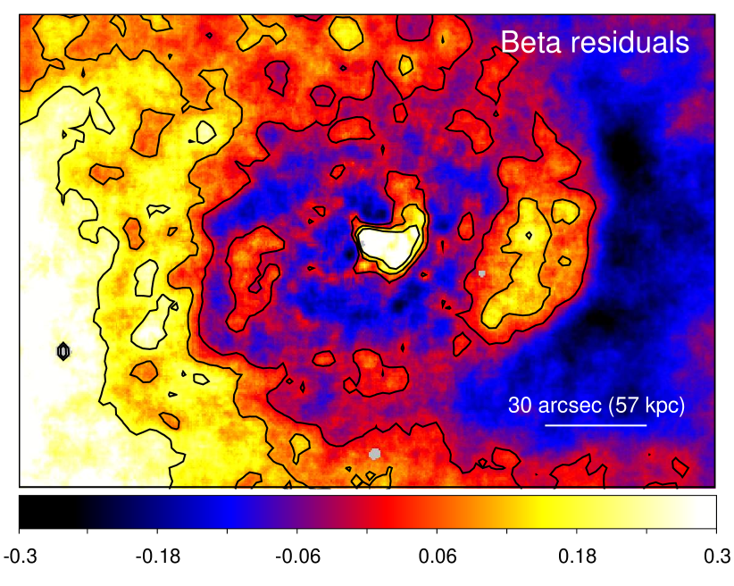
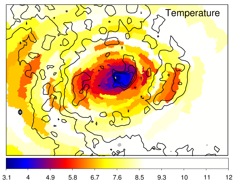
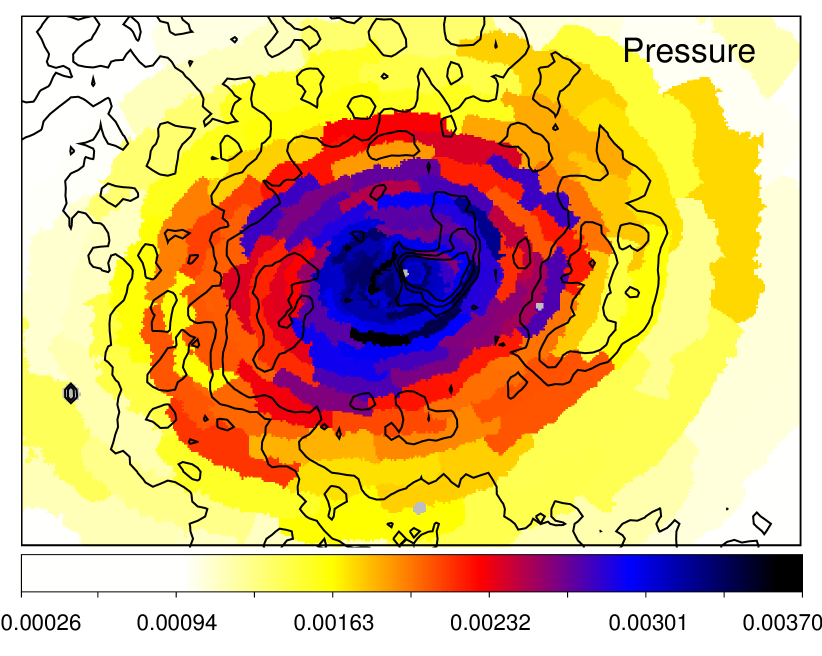
Figure 8: Spectral maps of the inner $206\times 136$ arcsec region ($\sim 390\times 260$ kpc). (Top panel) Image and contours are the fractional differences between an elliptical $\beta$ model fit to the surface brightness and an adaptively smoothed map. (Centre panel) Temperature map of the cluster, using bins with a signal to noise ratio of 66. (Bottom panel) Pseudo-pressure map of cluster, the square root of the mean surface brightness in each bin and multiplied by the temperature.

We now examine the properties of the ICM in the inner $390\times 260$ kpc. We fitted the spectra from bins with a signal to noise ratio of 66 ($\sim 4350$ counts). In these fits the absorbing column density and metallicity were allowed to be free parameters. In Fig. 8 (top panel) we show the fractional difference between the $\beta$ model fit to the cluster surface brightness (see Fig. 2) and an adaptively smoothed image of the cluster. The image was adaptively smoothed with a top-hat kernel dynamically adjusted to contain a signal to noise ratio of 30 (900 counts). The contours from this map are also plotted on this and the other panels. The middle panel shows the best fitting temperature. The uncertainties in this map range from 10 per cent per bin in the centre to 30 per cent in the hottest regions.

The surface brightness of the image is proportional to the integral of the density-squared along the line of sight (with a weak temperature factor, depending on the X-ray band chosen). If we bin the surface brightness into our spectral fitting regions, take the square root and multiply by the temperature, this gives a pseudo-pressure, related to an average of the pressure with a line of sight factor (bottom panel of Fig. 8). The pressure is asymmetric in the inner arcmin, with a difference in pressure of $\sim 30$ per cent between the north-west and south-east.

The central temperature map shows some features in common with the spiral structures seen in the residuals from the $\beta$ model. For instance there is a cool blob of material to the west of the core coincident with the brightest region of X-ray emission (Fig. 3). This region has lower pressure than other regions at similar radius. At larger radii beyond this western region is an edge in surface brightness, which we examine in more detail in Section 6.3. There is another smaller region of cooler material to the east, coincident with a smaller region of enhanced X-ray emission and lower thermal pressure.

6 Radial profiles

We investigate the radial profiles of several thermodynamic quantities. We compare the results of a new method, using multiband surface brightness projection against more conventional methods.

6.1 Multiband surface brightness projection

Our multiband surface brightness projection method (called MultiBand PROJector or mbproj) builds on the well-known surface brightness deprojection method of Fabian et al. (1981). It is similar to the recently published multiband projection model of Humphrey & Buote (2013) which analyses surface brightness profiles assuming functional forms for the mass distribution and entropy profile, inferring the density and temperature assuming hydrostatic equilibrium. Our technique differs by using a non-parametric density profile instead of a parametric entropy profile (although a parametric density profile can be used) and solves hydrostatic equilibrium by integrating the pressure inwards to the centre of the cluster. The aim of the method is to compute cluster thermodynamic property profiles from count profiles, without having to do spectral fitting and allowing high spatial resolution. As the code is forward-fitting, matching a model to observed data, we call this a projection method, rather than a deprojection method.

The data used by the procedure are count or surface brightness profiles in several energy bands. In our data analysis we used three bands. These bands should be chosen to contain sufficient counts and to be sensitive to temperature variation. For simplicity in this procedure, we assume that the surface brightness profiles are extracted from contiguous 2D annuli on the sky which have the same radii as the 3D shells in the cluster for which we model the thermodynamic properties. In addition, we assume constant values for the metallicity and Galactic absorption. The metallicity requirements can be broken by introducing parameters into the model representing its profile.

We assume the gravitational potential (excluding the contribution from X-ray gas mass) has a particular form, the cluster is in hydrostatic equilibrium and is spherical. To start our analysis, we take this potential (with initial parameters), an outer log pressure and an initial log electron density profile, assuming the density is constant within each shell. A separate density can either be given for each shell or generated parametrically, for example using a $\beta$ model. We then compute the surface brightness profile in several energy bands. This procedure is as follows.

1. The outer pressure and outermost density value is used to compute an outermost temperature.

2. The temperature, metallicity and density are converted into an emissivity for the outermost shell in the cluster in several energy bands. This calculation is done using xspec with the apec spectral model, given a response matrix and ancillary response matrix. For purposes of efficiency, the temperature to emissivity conversion is precalculated using a grid of temperature values for each band for unit emission measure. The calculation is done with zero and Solar metallicity, using interpolation to calculate the results using other metallicity values. The effects of Galactic photoelectric absorption are included in the emissivities, although this prevents modelling variation across the source.

3. We now consider the next innermost shell. We compute a pressure for this shell from the sum of the previous pressure plus the contribution from the hydrostatic weight of the atmosphere, i.e. $\delta P=\delta r\>\rho\>g$, where $\delta r$ is the radial spacing and $\rho$ is the mass density. $g$ is the gravitational acceleration computed from the potential in the shell plus a contribution to the acceleration from the gas mass of interior shells. $g$ for the potential is calculated at the gas-mass-weighted-average radius for the shell, assuming constant gas density

   $$r_{\mathrm{weighted}}=\frac{3}{4}\frac{(r_{\mathrm{in}}+r_{\mathrm{out}})(r_{\mathrm{in}}^{2}+r_{\mathrm{out}}^{2})}{r_{\mathrm{in}}^{2}+r_{\mathrm{in}}r_{\mathrm{out}}+r_{\mathrm{out}}^{2}},$$ (1)

   where $r_{\mathrm{in}}$ and $r_{\mathrm{out}}$ are the interior and exterior radii of the shell. To calculate the gas mass contribution to $g$, we calculate the total gravitational force on the shell from the mass of interior shells ($M_{\mathrm{int}}$) and from the shell itself, at constant density $\rho$. This is then divided by the total mass within the shell to compute an average acceleration,

   $$g_{\mathrm{gas}}=G\frac{3M_{\mathrm{int}}+\rho(r_{\mathrm{out}}-r_{\mathrm{in}})[(r_{\mathrm{out}}+r_{\mathrm{in}})^{2}+2r_{\mathrm{in}}^{2}]}{r_{\mathrm{in}}^{2}+r_{\mathrm{in}}r_{\mathrm{out}}+r_{\mathrm{out}}^{2}}.$$ (2)

4. Taking this pressure and the density value in this shell, we compute its emissivity in the several bands.

5. We go back to step 3 until we reach the innermost shell.

6. Given the emissivities for each shell, we compute the projected surface brightness in each band by multiplying by the volumes of each shell projected onto annuli on the sky and summing along the line of sight. We include the sky background by adding a constant onto each surface brightness profile.

Once we have the surface brightness profiles in each band for our choice of parameters (parameters of the gravitational potential, outer pressure and temperature profile) we can compare them to the observed surface brightness profiles. The projected surface brightness profiles are multiplied by the areas on the sky of each annulus and the exposure time of the observation to create count profiles. The exposure times can also include an additional factor from the average difference in an exposure map between the annulus and where the response matrices are defined, to account for detector features and vignetting. If sectors are examined within the cluster, rather than full annuli, this can be included within the area calculation, along with the negative contribution of any excluded point sources. To assess how well the model fits the data, we calculate the logarithm of the likelihood of the model for Poisson statistics (Cash, 1979) with

$$\log\mathcal{L}=\sum_{i}{\left[d_{i}\log m_{i}-m_{i}-\log\Gamma(d_{i}+1)\right]},$$ (3)

where $d_{i}$ and $m_{i}$ are the observed and predicted number of counts, respectively. $i$ indexes over each annulus in each band.

To obtain the initial density profile, we add the surface brightness profiles from all the energy bands and deproject the surface brightness profile assuming a particular temperature value (here 4 keV) and spherical symmetry. The initial outer pressure is the outer density times the temperature value. We then fit the complete set of parameters, including the potential parameters, by maximising $\log\mathcal{L}$ using a least-squares minimisation routine. The basin-hopping algorithm (Wales & Doye, 1997) is then employed to help ensure that the fit is not in a local minimum.

We start an MCMC analysis to obtain a chain of parameter values after a burn-in period. We again use emcee for the MCMC analysis. The initial parameters for the walkers are set to be tightly clustered around the best fitting parameters. Flat priors are used on all parameters. After the run, uncertainties on the parameters can be obtained by computing the marginalised posterior probabilities from the chain for each parameter. To compute radial profiles of other thermodynamic quantities, we take sets of parameters from the chain and compute the quantity for each set of parameters and examine the distribution of these output values. We compute the electron density, electron pressure, electron entropy (defined as $K_{\mathrm{e}}=n_{\mathrm{e}}T^{-2/3}$), cumulative gas mass, cumulative luminosity, mean radiative cooling time, cumulative mass deposition rate in the absence of heating (accounting for the gravitational contribution; Fabian 1994), gravitational acceleration, total cumulative mass and gas mass fraction.

6.1.1 Rebinning input profiles

The sizes of the input annular bins must be chosen in some way. When fitting for separate densities in each shell, there is one density parameter per shell. To reduce the uncertainties on the densities, the input profiles need to be binned. In principle, if a functional form is assumed for the density profile then the input profiles do not need binning, but in practice to get a good initial density estimate, some binning is required.

A second code, mbautorebin, is used to rebin the profiles before analysis. We take initial count profiles for each band, computed using pixels. The profiles are added to give a total count profile. The method works inwards from the outside of the profile. Radial annular bins are combined until the fractional uncertainty on the emissivity in the respective 3D shell drops below a threshold and the total number of counts in the shell is greater than a second threshold. Once the threshold is reached, we then consider the next innermost bin.

The emissivity in a shell is computed by deprojecting the counts in each annulus assuming spherical symmetry. To be precise, to calculate the emissivity, the projected contributions from the background and already binned 3D shells is subtracted from the count rate for the annulus, and this rate is then divided by the volume of the shell within the annulus. Monte Carlo realisations of the count rate in the shell and those shells outside are used to estimate the uncertainty.

For the central remaining bin after this process, we combine it with the next innermost bin if the uncertainty on the emissivity is substantially below the threshold.

There may be some form of bias generated from this procedure if the number of counts is very low. Bin sizes may depend on the radii of particular counts. In the low count regime (a few hundred counts or less), we used an alternative version of this code which fits a $\beta$ model to the surface brightness profile. The bin radii are adjusted to give the same fractional uncertainty on the deprojected emissivity in each bin, based on realisations of the $\beta$ model.

6.1.2 Null potential case

The above procedure can be modified to compute thermodynamic profiles without the assumption of hydrostatic equilibrium. We term this adaptation of the model the Null potential case. Here we add parameters for the temperature in each shell and do not use the gravitational potential. Rather than calculating the pressure assuming hydrostatic equilibrium, we multiply the temperature and density values. This variation of the model is in essence a low-spectral resolution version of spectral fitting projection models, such as projct. It provides a useful check to ensure that the thermodynamic profiles are not being biased by the choice of gravitational potential or by parts of the cluster being out of hydrostatic equilibrium.

6.2 Complete radial profiles

To examine the average cluster profiles, we extracted count profiles for the cluster from images in the 0.5 to 1.2, 1.2 to 2.5 and 2.5 to 6 keV bands out to a radius of 4.55 arcmin (516 kpc). The profiles were extracted on a pixel-by-pixel basis and the areas calculated by summing numbers of pixel. A 0.5 to 7 keV exposure map was used to correct the areas for bad pixels and other detector features. We restricted the analysis to region covered by the ACIS-S3 CCD for the 12881 observation, excluding point sources. In addition to using standard background event files to obtain the X-ray and particle backgrounds, we account for out-of-time events which occur during detector readout using the make_readout_bg script of M. Markevitch to generate out-of-time event files. Out-of-time events would otherwise lead to regions along the readout direction being contaminated with emission from the centre of the cluster. PKS0745 has a bright central core, making this problem more obvious. We extracted surface brightness profiles from both background event files, combining them. The foreground and background input profiles were rebinned to obtain a maximum deprojected emissivity error of 4 per cent. This gives around 20 000 projected counts per radial bin over most of the radial range, reducing to around 10 000 near the outskirts.

Table 3: Details of the MCMC analysis of the various data and samples. Shown are the data analysed, the potential used, the maximum log likelihood, number of walkers used, burn length used, sample length used, acceptance fraction, mean autocorrelation period ($\langle\tau\rangle$) and maximum autocorrelation period ($\max\tau$).

Region	Potential	$\max\log\mathcal{L}$	Walkers	Burn	Length	Acceptance	$\langle\tau\rangle$	$\max\tau$
Full	NFW	$-941.7$	200	1000	4000	0.18	134	311
	King	$-865.8$	200	1000	4000	0.18	131	302
	Arb4	$-861.7$	400	2000	8000	0.18	214	591
	Null (bin 2)	$-846.2$	400	2000	8000	0.15	259	611
	Null	$-833.9$	800	8000	90000	0.08	2170	5293
	NFW $>0.5^{\prime}$	$-638.8$	200	1000	4000	0.20	118	282
	King $>0.5^{\prime}$	$-636.7$	200	1000	4000	0.21	116	295
West	NFW	$-451.4$	200	1000	4000	0.22	110	294
	King	$-448.8$	200	1000	4000	0.22	102	277
East	NFW	$-445.7$	200	1000	4000	0.21	113	297
	King	$-445.0$	200	1000	4000	0.21	109	291

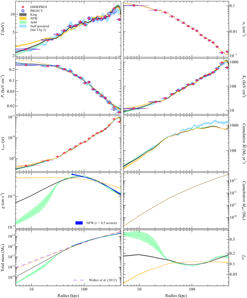
Figure 9: Complete radial profiles, comparing analysis methods. Shown are the results for spectral fitting using dsdeproj and projct, and mbproj with several mass models, including a King, an NFW, a 4 bin parametrisation (Arb4) and a null potential (fitting densities instead). The quantities shown include the temperature ($T$), electron density ($n_{\mathrm{e}}$), electron pressure ($P_{\mathrm{e}}$), electron entropy ($K_{\mathrm{e}}$), mean radiative cooling time ($t_{\mathrm{cool}}$), cumulative mass deposition rate ($\dot{M}$), gravitational acceleration ($g$) and cumulative gas mass ($M_{\mathrm{gas}}$). In the $g$ and total mass plots we also show the results for an NFW model which only examines the data outside 0.5 arcmin radius. For the total mass panel, we show the mass profile obtained from Suzaku data by Walker et al. (2012).

Several different potential models were examined using mbproj, with the results shown in Fig. 9. The central lines show the median parameter values taken from the chain, with shaded bar showing the uncertainties taken from the 15.9 and 84.1 percentiles, equivalent to $1\sigma$ errors. The potentials used were an NFW model (Navarro, Frenk & White, 1996), a King model (King, 1962), the null potential and an arbitrary potential, Arb4, where we parametrised the mass density at 4 logarithmically spaced radii over the radial range and used linear interpolation and integration to compute the gravitational acceleration. We assumed a metallicity of $0.4\hbox{$\thinspace\mathrm{Z}_{\odot}$}$ and an absorbing column density of $3.78\times 10^{21}\hbox{$\rm\thinspace cm^{-2}\,$}$, based on an average of values from fitting bins over the cluster core. For the null potential model we show the results where there is a single temperature parameter in each shell and one where the temperatures in each pair of bins is assumed to be the same (bin 2).

The details of the MCMC analysis are shown in Table 3. We show log likelihoods for the best fitting parameters, the number of walkers used, the burn period, the length of the final chain. The acceptance fraction of the chain is shown. Ideally this should be between 0.2 and 0.5 (Foreman-Mackey et al., 2012). Low values, as seen in the null potential model with a single temperature parameter for each bin, may indicate multi-modal parameter values which are difficult for the MCMC analysis to sample.

Table 4: Derived marginalised posterior probabilities for the parameters on the potentials from the surface brightness analysis. For the Arb4 model the density units are $\log_{10}10^{-24}\hbox{$\rm\thinspace g\rm\thinspace cm^{-3}\,$}$.

Potential	Parameters
NFW	$c=3.88\pm 0.14$	$r_{200}=(2.20\pm 0.06)\rm\thinspace Mpc$
King	$\sigma=(769\pm 9)\hbox{$\rm\thinspace km\rm\thinspace s^{-1}\,$}$	$r_{\mathrm{core}}=(83\pm 2)\rm\thinspace kpc$
Arb4	$\rho_{1}=-1.0^{+0.3}_{-0.6}$	$\rho_{2}=0.05^{+0.05}_{-0.04}$
	$\rho_{3}=-0.45\pm 0.03$	$\rho_{4}=-1.80\pm 0.08$
NFW ($r>0.5^{\prime}$)	$c=9.2_{-0.8}^{+0.5}$	$r_{200}=1.42_{-0.03}^{+0.05}\rm\thinspace Mpc$
King ($r>0.5^{\prime}$)	$\sigma=(760\pm 12)\hbox{$\rm\thinspace km\rm\thinspace s^{-1}\,$}$	$r_{\mathrm{core}}=(78\pm 6)\rm\thinspace kpc$

For models with more parameters (the Null and Arb4 models), we increased the number of walkers in the analysis. Table 3 also shows the mean and maximum autocorrelation periods ($\tau$) for parameters from individual walkers in the chain. To properly sample parameter values so that the chain has converged, the chain should be $\sim 10$ times longer than this period (Foreman-Mackey et al., 2012). This is the case on our analyses. The null models have long autocorrelation periods, likely due to the multivalued temperatures at larger radii, and so required much longer chain lengths. The derived marginalised posterior probabilities for the mass models are given in Table 4.

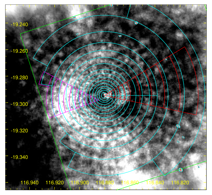
Figure 10: $\beta$-model-residual image showing the annular sectors used for the dsdeproj and projct spectral analyses of the whole azimuthal range and the western and eastern sectors. The rotated box shows the edge of the ACIS-S3 CCD in the 12881 observation. The X-ray image was adaptively smoothed to have a signal to noise ratio of 15 in the smoothing kernel and was then divided by an elliptical $\beta$ model fit.

To compare the results from our analysis, we also examined the results of spectral fitting using two different methods for account for projection effects. The first method was to use the dsdeproj code to deproject projected spectra (Sanders & Fabian, 2007; Russell, Sanders & Fabian, 2008). We also used the projct model in xspec, which projects spectra. The radii of the annuli chosen were the surface brightness deprojection bins, but binned up by a factor of three (Fig. 10). We note that for these spectral fits, we fixed the column density to the same value as the surface brightness deprojection. The metallicity of each shell, however, was free in the spectral fits. The spectra were fitted between 0.5 and 7 keV. For projct, all the spectra were fitted simultaneously to minimise the total $\chi^{2}$ (the reduced $\chi^{2}$ was $1.02=6447/6321$).

The spectral results are compared with the data in Fig. 9. There appears to be good agreement between the spectral fitting results and our deprojection code. However, there is a discrepancy in the temperature and pressure results at small and large radius between the NFW analysis and the other results. Examining the gravitational acceleration, $g$, the Arb4 gravitational model appears to match the King model fairly well except at small radii, but matches the NFW model poorly. If we exclude the central region from the data and only fit the data beyond 0.5 arcmin radius, the NFW model matches the other models much better in that region (bottom left two panels of Fig. 9).

Similar results to the Arb4 model are also found with a model where the gravitational acceleration is parametrised in 6 logarithmic radial intervals, using linear interpolation to calculate intermediate values. In this case, the gravitational acceleration is unconstrained inside 10 kpc radius, but $g$ is similar to the Arb4 model elsewhere.

We also note that the null potential model shows different mass deposition rates ($\dot{M}$) compared to the other models because it does not include the gravitational contribution. Both the spectral and projection methods have anomalous values in their outer bins. This is due to cluster emission outside these radii not being taken into account.

6.3 Surface brightness edges

In the western half of the cluster, there are two edges visible in the X-ray surface brightness (Fig. 2). We have analysed the thermodynamic properties across these edges by spectral fitting and by applying mbproj. The sectors we used for the spectral fitting are shown in Fig. 10. The same azimuthal and radial ranges were used for the surface brightness analysis. The edges of the spectral extraction regions were chosen to match the edges in surface brightness as closely as possible. We analysed the data similarly to Section 6.2 but using a column density of $4.27\times 10^{21}\hbox{$\rm\thinspace cm^{-2}\,$}$. This increased value was necessary due to the westward rise in column density (Section 7) and was obtained as the best fitting value from the projct analysis. The surface brightness profiles were rebinned in radius to have a minimum uncertainty on the emissivity of 6 per cent. We used both King and NFW mass models in our mbproj analysis.

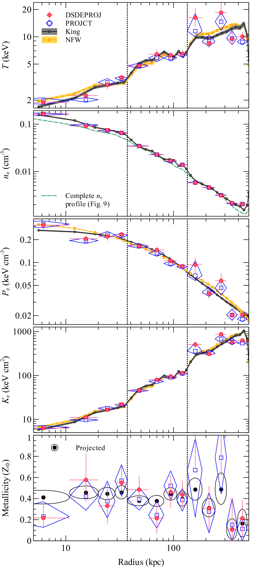
Figure 11: Profiles to the west of the core across the two surface brightness edges, of temperature, electron density, electron pressure, electron entropy and metallicity. The positions of the edges are marked by dotted lines. Shown are the results for spectral fitting (dsdeproj, projct and Projected for metallicity) and using mbproj (with NFW and King potentials). The complete cluster results from Fig. 9 are also plotted with the electron density profile.

The profiles in this sector are shown in Fig. 11. The results show that there are two obvious breaks in density, temperature and entropy at the locations of these edges. The mbproj results suggest that the breaks have finite width, although any perturbations in the shape of the edge relative to our extraction region will broaden its measured width. The spectral fitting results indicate that there may be a break in pressure at the innermost edge. Using the mbproj method, there can never be a discontinuity in pressure as a hydrostatic atmosphere is assumed. The spectral fitting pressure inside the edge are enhanced with respect to the smooth curves. Considering only the two points either side of the edge, the pressure jump relative to the smooth curves is around $2\sigma$ in significance. However, if powerlaw models were fitted inside and outside the edge, then the significance of the break would increase. The metallicity profile in the centre is remarkably flat at $0.4\hbox{$\thinspace\mathrm{Z}_{\odot}$}$ within 300 kpc radius.

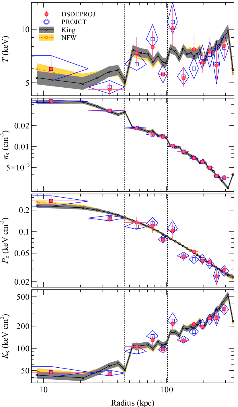
Figure 12: Profiles of quantities to the east of the cluster core, across two surface brightness edges, marked by vertical lines. Note that the centre of this deprojection is offset 20 arcsec south-east of the core (38 kpc), to better match the sector to the edges. We show results for spectral fitting (dsdeproj and projct) and mbproj using NFW and King potentials.

We similarly examined the properties of the cluster in the eastern direction across the surface brightness edges (Fig. 12). This is more difficult because the edges are not smooth or centred on the cluster nucleus. They appear to look rather kinked (Fig. 2), similar to those seen in seen in Abell 496 (Roediger et al., 2012). We have therefore examined the deprojected profiles using a sector with a centre offset around 40 kpc south west from the core of the cluster (Fig. 10), so that the circular sectors better match the surface brightness features. This introduces systematic geometric error into the analysis. The radial features, however, are also seen in projected profiles. We repeated the same spectral and mbproj analyses as in the western sector, but rebinning the input profiles to give a minimum uncertainty of 10 per cent on the emissivity.

We again see density, temperature and entropy jumps across the two edges (although the outer temperature jump is less significant). The pressure does not appear to jump at the edges. Fig. 10 shows a further reduction with surface brightness near the edge of our sector (at radii of $\sim 240$ kpc from the cluster core) associated with the spiral structure. Unfortunately this edge lies close to the boundary between two neighbouring CCDs, making it difficult to examine both in terms of surface brightness and spectrally.

7 Larger scale maps

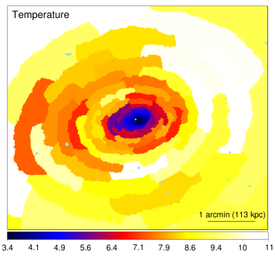
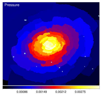
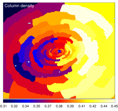
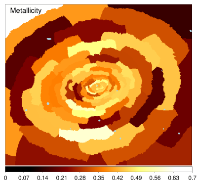
Figure 13: Maps of the temperature in keV (top-left), pseudo-pressure (top-right), absorbing column density in $10^{22}\hbox{$\rm\thinspace cm^{-2}\,$}$ (bottom-left) and metallicity in Solar units (bottom-right) on large scales. The cluster was binned to have regions with a signal to noise ratio of 101 ($\sim 10^{5}$ counts).

Fig. 13 shows larger scale maps of the properties of the ICM in the cluster. To produce these maps we fitted spectra from bins with a signal to noise ratio of 101 (10200 counts). We use a single component APEC model, allowing the temperature, metallicity, normalisation and absorbing column density to be free in the fits. In addition to extracting background spectra from standard-background-event files, spectra were extracted from the out-of-time-event files for each bin, combining the datasets. In xspec they were loaded as a correction file during spectral fitting for each bin. Input spectra were grouped to have a minimum of 20 counts per spectral bin. We fit the spectra between 0.5 and 7 keV, minimising the $\chi^{2}$ of the fit. The resulting maps show that there is considerable variation in absorbing column density across the image. The variation is in the direction of galactic latitude, with stronger absorption towards the Galactic plane. As PKS0745 is near the galactic plane, this suggests that the variation could be real, as implied by the large standard deviation of the nearby LAB values. Alternatively, the variation could be due to calibration, for example uncorrected contaminant on the ACIS detector. Analysis of XMM data would confirm whether it is real. There are also non-radial variations in temperature and pressure, which we examine further in the following section.

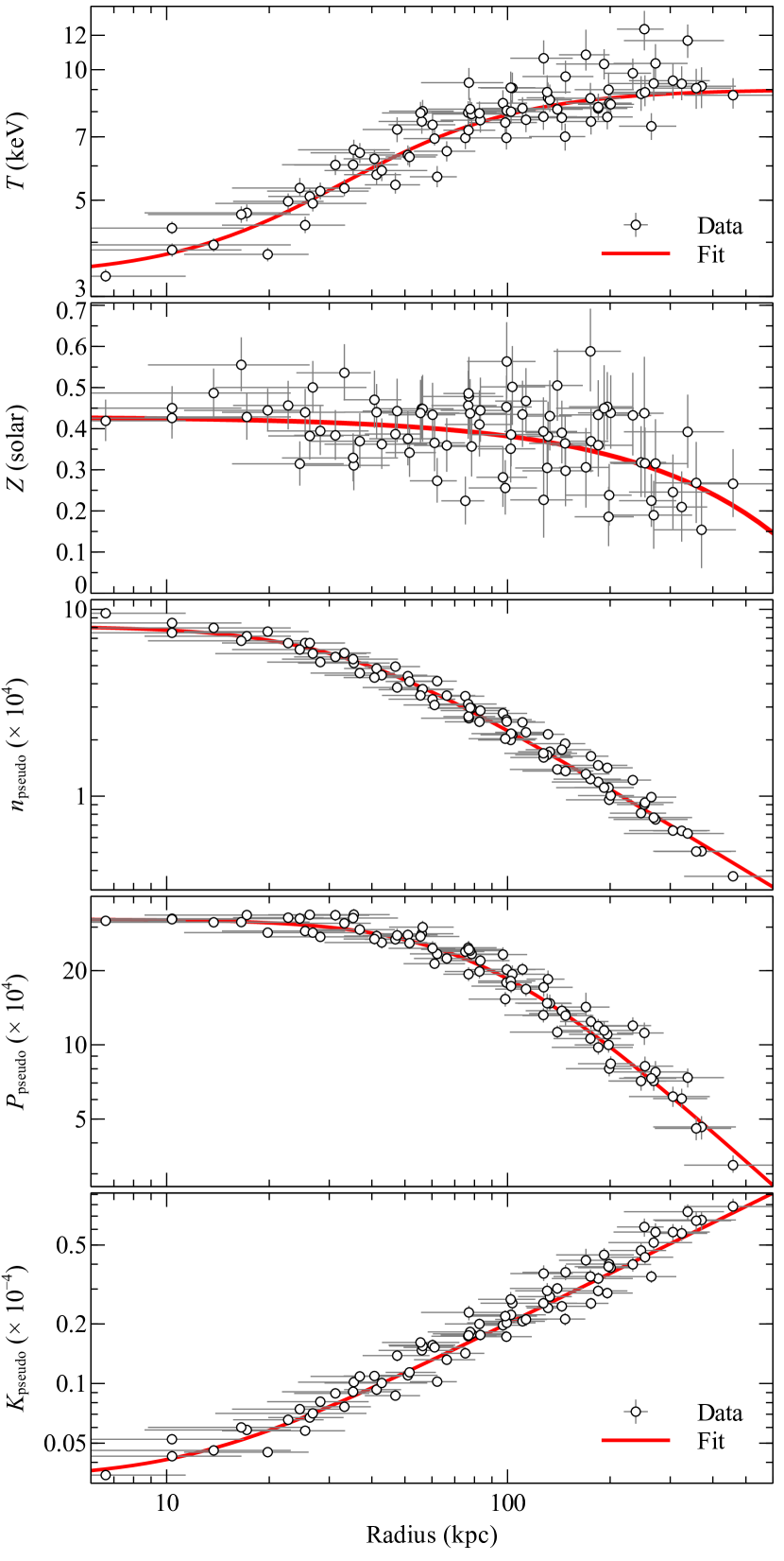
Figure 14: Profiles generated from the maps in Fig. 13. The value of the bin is plotted against the mean bin position. The radial error bars show the bin extents. The quantities are temperature (1st panel), metallicity (2nd panel), pseudo-density (3rd panel), pseudo-pressure (4th panel) and pseudo-entropy (5th panel).

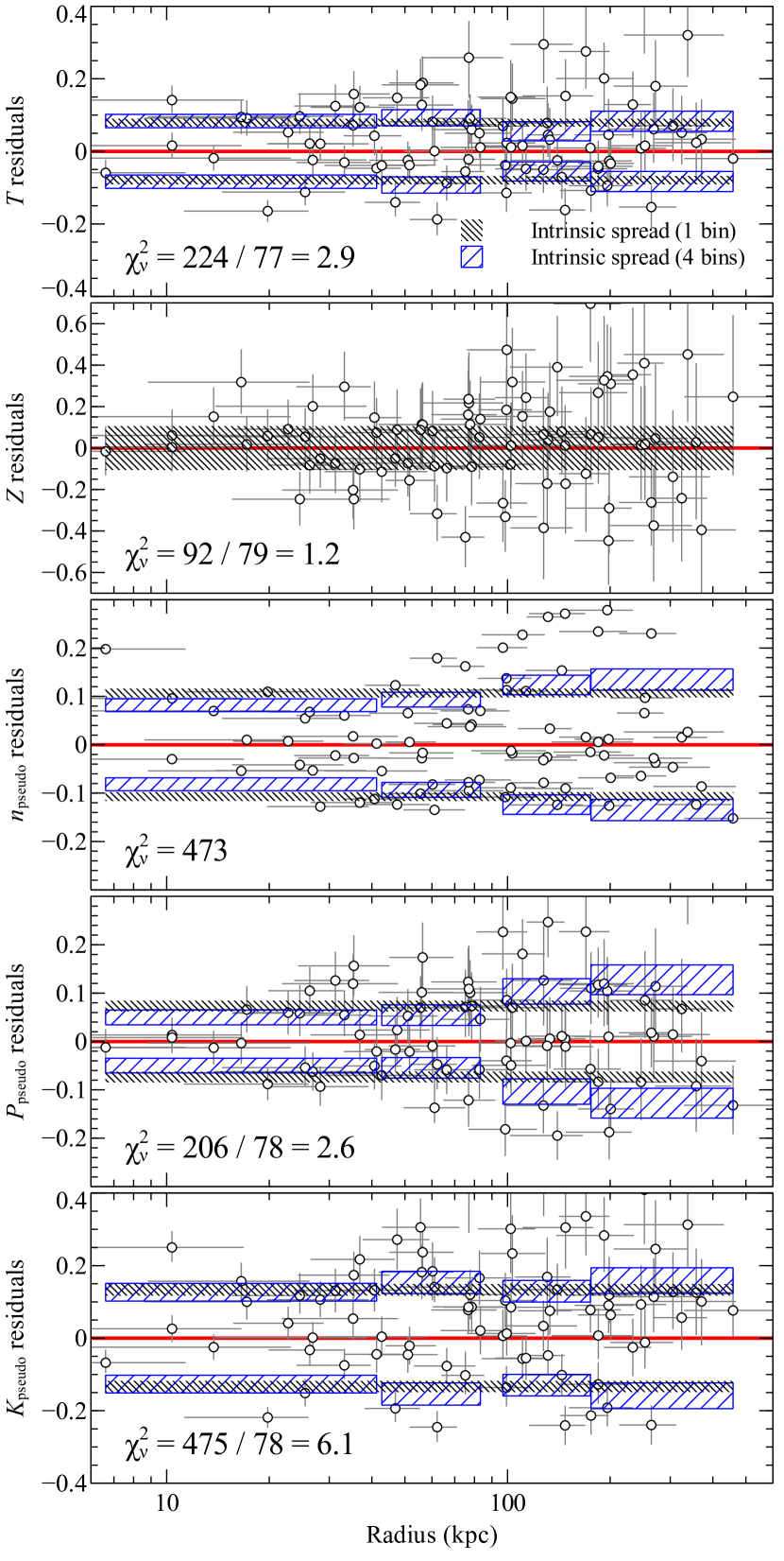
Figure 15: Fractional residuals to the best fitting models in Fig. 14 with the intrinsic dispersion of the points shown. The numeric value show is the reduced-$\chi^{2}$ of the fit. The intrinsic dispersion is shown for all points (finely hatched region) and using four radial bins containing equal numbers of points (coarse hatched region), except for the metallicity plot which shows no significant dispersion when split into separate regions. The dispersion shows the range of additional dispersion which is consistent with Monte Carlo realisations of the best fitting models.

7.1 Fluctuations in quantities

The energy in turbulent fluctuations, generated during the growth of a cluster, is predicted to increase from a few per cent of the thermal energy density in the centre of a relaxed cluster to tens of per cent in its outskirts (Vazza et al., 2009, 2011; Lau, Kravtsov & Nagai, 2009). Unrelaxed objects, such as those which have previously undergone a merger, have more turbulent energy at all radii, but particularly in the central region where it may reach tens of per cent. In addition, the central AGN may generate motions (Brüggen, Hoeft & Ruszkowski, 2005; Heinz, Brüggen & Morsony, 2010). With current instrumentation it is possible to directly measure or place limits on turbulent motions in some cases (see Sanders & Fabian, 2013). However, the spectra of fluctuations in surface brightness and therefore density can be measured from images and used as an indirect probe of turbulence (Churazov et al., 2012; Sanders & Fabian, 2012; Zhuravleva et al., 2014). By the choice of energy band for particular temperature ranges, it is possible to examine pressure fluctuations using surface brightness (Sanders & Fabian, 2012). Simulations indicate that density variations can be used to infer the magnitude of turbulence (Gaspari et al., 2014).

Here, rather than purely relying on surface brightness, we use spectral information to measure the non-radial dispersion of various interesting thermodynamic quantities (temperature, density, pressure and entropy) as a function of radius relative to smooth models. Measuring these quantities directly provides useful constraints on turbulence without assuming the results from simulations.

In Fig. 14 are shown the values of the temperature ($T$), metallicity ($Z$), pseudo-density ($n_{\mathrm{pseudo}}$), pseudo-pressure ($P_{\mathrm{pseudo}}$) and pseudo-entropy ($K_{\mathrm{pseudo}}$) for each bin as a function of the average radius of the bin. We exclude two large bins in the outskirts which cover a very large radial range. Pseudo-density is the square root of the surface brightness, which is roughly proportional to density times a line of sight length. We define the pseudo pressure and entropy as $P_{\mathrm{pseudo}}=T\,n_{\mathrm{pseudo}}$ and $K_{\mathrm{pseudo}}=T\,n_{\mathrm{pseudo}}^{-2/3}$, respectively. The solid lines show radial model fits to the data points, obtained by minimising the $\chi^{2}$ statistic. For the temperature profile we fitted the ‘universal’ temperature profile of Allen, Schmidt & Fabian (2001). A simple linear function was fitted to the metallicity, a $\beta$ model to the pseudo-density and pseudo-pressure, and a $\beta$ model with a negative index to the pseudo-entropy. It can be seen that there are large amounts of scatter at each radius in some of these quantities, although the error bars on the metallicities are large. To demonstrate this, we plot the fractional residuals of each fit to the data in Fig. 15 and quote the $\chi^{2}$ of the fit.

Table 5: Calculated intrinsic fluctuations in the bin maps over the entire radial range, before removing projection effects. The correction column shows whether radial symmetry is assumed (No) the elliptical elfit surface brightness correction has been applied (SB elfit) or the correction from fitting an elliptical $\beta$ model to the pressure and density maps (Pressure $\beta$ and Density $\beta$). Projection effects are likely to increase these values by a factor of $\sim 2$ (Section 7.5).

Quantity	Correction	Dispersion
$T$	No	$0.07\pm 0.01$
$Z$		$<0.1$
$n_{\mathrm{pseudo}}$		$0.11\pm 0.01$
$P_{\mathrm{pseudo}}$		$0.07\pm 0.01$
$K_{\mathrm{pseudo}}$		$0.13\pm 0.02$
$T$	SB	$0.05\pm 0.01$
$Z$	(elfit)	$<0.1$
$n_{\mathrm{pseudo}}$		$0.018\pm 0.002$
$P_{\mathrm{pseudo}}$		$0.05\pm 0.01$
$K_{\mathrm{pseudo}}$		$0.06\pm 0.01$
$T$	Pressure	$0.10\pm 0.01$
$Z$	($\beta$)	$<0.1$
$n_{\mathrm{pseudo}}$		$0.069\pm 0.006$
$P_{\mathrm{pseudo}}$		$0.03\pm 0.01$
$K_{\mathrm{pseudo}}$		$0.16\pm 0.02$
$T$	Density	$0.10\pm 0.01$
$Z$	($\beta$)	$<0.1$
$n_{\mathrm{pseudo}}$		$0.069\pm 0.006$
$P_{\mathrm{pseudo}}$		$0.03\pm 0.01$
$K_{\mathrm{pseudo}}$		$0.16\pm 0.02$

The points will contain some spread due to measurement errors and a contribution from the intrinsic fluctuations in the cluster at each radius. We can calculate the intrinsic dispersion, assuming that the points follow the fitted radial models. We make Monte Carlo simulations of the quantities assuming that points have the error bars measured in the data plus an additional fractional dispersion, added in quadrature. The fraction of simulations which have a fit statistic better than the real fit statistic is calculated as a function of the dispersion value. From the dispersion values where the fraction of better fitting simulations is 0.50, 0.159 and 0.841 of the total, we calculate the best fitting dispersion and its uncertainties. These values are shown for all the points in Fig. 15 and in four radial bins, excluding the metallicity profile. The average values for the additional dispersion of the quantities are given in Table 5. The residual profiles appear rather flat, although there may be some increase in the scatter of density and pressure with radius. We do not detect significant scatter in metallicity.

7.2 Correcting for surface brightness ellipticity with elfit

The cluster has an elliptical morphology (Fig. 2). This will give rise to some of the azimuthal variation of the quantities, even if the data points were intrinsically smooth. To examine the effect of the ellipticity, centroid shifts and isophotal twisting, we again applied the same elfit model with a series of 20 ellipses fitted to the contours in surface brightness at logarithmic surface brightness contours. We firstly created a corrected radius map, where for each pixel in the image we calculated the smallest distances to the nearest two ellipses and calculated the pixel radius by linearly interpolating between the average radii of those ellipses. Given this radius image, we gave each bin in the spectral map a radius from the average radius of the bin pixels in the corrected radius map. This procedure reduces the effects of isophotal twisting and edges from the data points.

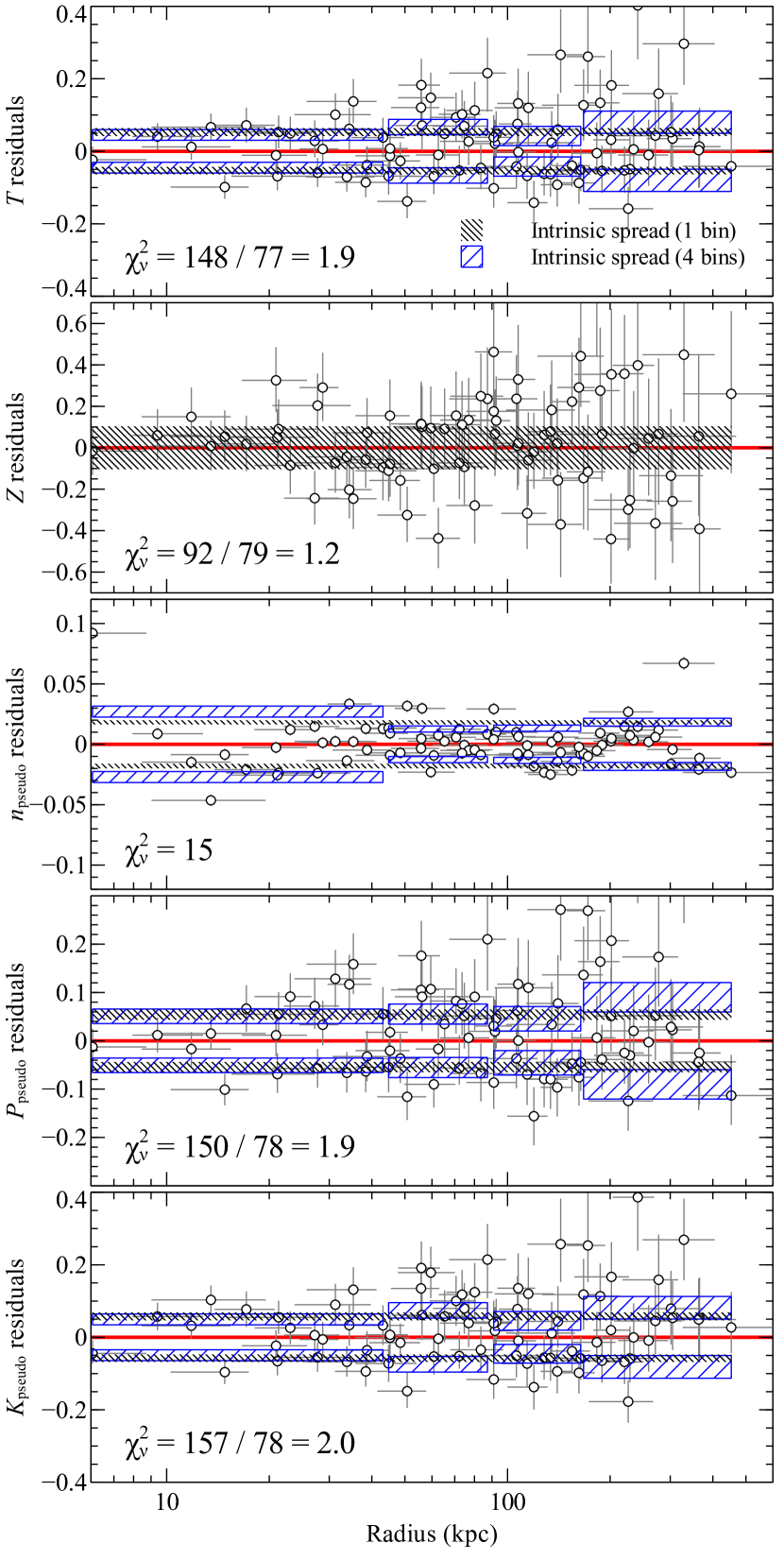
Figure 16: Fractional residuals to the data points after correcting the bin radii for the surface brightness ellipticity of the cluster on the sky. See Fig. 15 for the points before correction. Notice the change in axis scale for $n_{\mathrm{pseudo}}$. Large systematic variations were visible in the density residuals after correction. By using a double-$\beta$ model, we removed many of these variations.

Fig. 16 shows the residuals from the fits after correcting the bin radii for elliptical variations. The scatter on all the quantities except pressure is significantly reduced after this correction (Table 5). For the density fit, a second $\beta$ model component was added to the fit to remove significant radial residuals. The radial profiles of scatter are again rather flat, but the density plot shows low scatter ($\sim 2$ per cent with projection) in the middle of the radial range, with larger deviations in the centre. The central deviations are likely to be due to the AGN activity.

7.3 Pressure and density correction with elliptical $\beta$ models

If the cluster is in hydrostatic equilibrium, the pressure map is unaffected by local density or temperature perturbations. Therefore the pressure map may better indicate the morphology of the cluster potential than the density or surface brightness. To investigate whether the scatter in the thermodynamic quantities is reduced after correcting for the pressure map, we fitted the projected pressure map by an elliptical $\beta$ model. We minimised the $\chi^{2}$ between our model and the data assigning an uncertainty to each pixel of the total for that bin, divided by $\sqrt{n_{\mathrm{pix}}}$, where $n_{\mathrm{pix}}$ is the number of pixels in the bin. The outermost very large bins were excluded.

We obtain an ellipticity for the pressure map of $0.25\pm 0.03$ (i.e. a ratio between the minor and major axes is $0.75$) and find the major axis is inclined $17\pm 3$ degrees north from the west. The centre of the model is offset by about 6 arcsec from the nucleus to the south-east. The pseudo-density map has a similar ellipticity of $0.27$, inclined northwards by 13 degrees. By comparing the ellipticity of the pressure and density, if the cluster is in hydrostatic equilibrium, it would be possible to estimate the ellipticity of the dark matter potential. Fixing the ellipticity and angle in the pressure fit to the best fitting density values increases the $\chi^{2}$ by only 2.4, showing that the difference is not significant. We do not see any evidence for an elliptical dark matter potential. However, a gravitational potential is much more symmetric than the underlying matter density, so measuring this difference is difficult.

Similarly for the elliptical surface brightness correction, we can adjust the radii of pixels to correct for the ellipticity of the pressure distribution. Table 5 (under Pressure, $\beta$) shows that the pressure fluctuations are reduced to around 3 per cent. The density fluctuations also appear to be reduced compared to the spherically-symmetric case, but the temperature and entropy variations are increased.

However, we cannot compare the fluctuations from the pressure $\beta$ modelling to the surface brightness elfit results, because the $\beta$ correction is relatively crude. It does not, for example, remove isophotal twisting, centroid shifts or a changing ellipticity as a function of radius. If we repeat the analysis, fitting the density map with an elliptical $\beta$ model and doing the radial correction, we obtain exactly the same results as with the pressure map (Table 5 under Density, $\beta$). This confirms that the density and pressure ellipticities are very similar.

7.4 Dependence on bin size

The magnitude of the fluctuations will have some dependence on the bin size, as features below the bin size will be smoothed out. We investigated using bins using a signal to noise ratio of 66 instead of 100 (around 70 per cent of the linear dimension). The computed additional fluctuations were consistent with each other.

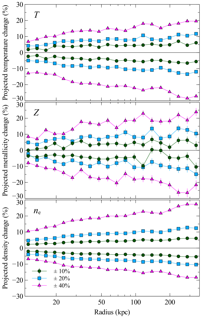
Figure 17: How projection effects affect the measurement of fluctuations in quantities as a function of radius. Using simulations, fluctuations were inserted in the cluster at a particular radius. We assume a bin size equivalent to a signal to noise ratio of 100 at a radius and assume the depth of the fluctuation along the line of sight is that radius. The values show the measured average change in the projected quantity on the sky.

7.5 Projection effects

The measured dispersions are projected quantities. The intrinsic dispersion in the cluster itself will be larger, as fluctuations are smoothed out by the projected emission. We therefore simulated the effects of projection on fluctuations. From the deprojected profiles in Section 6, we calculated the projected surface brightness as function of radius on the sky. This quantity was then converted to the projected bin size giving a signal to noise ratio of 100, assuming a square bin. For the unperturbed case, at that radius on the sky, we simulated the spectrum along the line of sight in that bin, by adding together simulated spectra in slices out to a cluster radius equivalent to 4.5 arcmin on the sky. We assumed each slice has constant properties, measured at its midpoint. From this total spectrum, the best fitting temperature, metallicity and normalisation was found. The simulation was repeated 160 times to calculate the mean values and their uncertainties. We then enhanced or reduced one of the cluster properties (temperature, metallicity or density) along the line of sight within half the cluster-bin radius from the cluster midplane. The best fitting quantities were compared to their baseline values to examine the effect of projection.

Fig. 17 shows the measured percentage increase or decrease in temperature, metallicity or density (half the normalisation change), when the intrinsic cluster emission is varied. We examine variations in quantities of 10, 20 and 40 per cent. These profiles show that projection effects are worst in the centre of the cluster, despite the rising surface brightness profile. The measured fractional reduction in fluctuation are reasonably consistent between the different quantities. The strength of measured fluctuations is reduced to around 25 per cent in the centre of the cluster, increasing to 50 per cent at a few hundred kpc. As pressure and entropy are combinations of temperature and density, they should have similar correction factors.

Note that in reality we do not know the length of fluctuations along the line of sight, although the radius on the sky is probably a reasonable approximation. For comparison, if we instead assume the unlikely case that the fluctuations are concentrated in the midplane of the cluster and that they are only a bin width thick, we would obtain fairly uniform projection factors of around 25 per cent in all quantities.

8 Discussion

8.1 Cooling and heating in the cluster core

PKS0745 hosts a galaxy cluster where there is evidence for cooling in many different wavebands. Defining the cooling radius to be the radius where the mean radiative cooling timescale is less than $7.7\rm\thinspace Gyr$ (the time since $z=1$), it is 115 kpc in PKS0745 (Fig. 9). Within this radius the cumulative mass deposition rate calculated from the surface brightness profiles, taking into account the gravitational work done, is $730\hbox{$\hbox{$\rm\thinspace M_{\odot}$}\rm\thinspace yr^{-1}\,$}$. This would be the steady-state cooling rate in the absence of any form of feedback. Examining the Chandra spectrum inside this radius, we find it consistent with $112\pm 2\hbox{$\hbox{$\rm\thinspace M_{\odot}$}\rm\thinspace yr^{-1}\,$}$ cooling from 6.7 to 0.2 keV temperature (Table 1). The RGS instruments on XMM are more suitable for this measurement, although existing observations are short. However, fixing the model metallicity at the Chandra value, we find consistent results of $270\pm 90\hbox{$\hbox{$\rm\thinspace M_{\odot}$}\rm\thinspace yr^{-1}\,$}$ (Table 2). The minimum temperature in this case is $0.5_{-0.2}^{+0.1}$ keV. Splitting the spectrum into temperature bins (Fig. 7), the Chandra and XMM spectra are largely consistent in showing the spectra are consistent with rates of $\sim 300\hbox{$\hbox{$\rm\thinspace M_{\odot}$}\rm\thinspace yr^{-1}\,$}$ between 4 and 0.5 keV. Below 0.5 keV, the results are inconsistent, although measuring such cool components with Chandra is very difficult due to effective area, spectral resolution and calibration uncertainties. In addition, the cluster has a large Galactic column. Forthcoming XMM observations will enable us to examine the X-ray spectrum in more detail.

Deep observations of several cooling flow clusters have shown that the picture of a complete cut off in the X-ray temperature distribution is incorrect. There are many cases now showing clusters with cool X-ray emitting gas embedded in a hotter medium, associated with emission line filaments, including Centaurus (Sanders et al., 2008), Abell 2204, (Sanders, Fabian & Taylor, 2009b), 2A 0335+096 (Sanders, Fabian & Taylor, 2009a), Abell 2052 (de Plaa et al., 2010), M87 (Werner et al., 2010), Sérsic 159 (Werner et al., 2011), Abell 262 and Abell 3581 (Sanders et al., 2010) and in several elliptical galaxies (Werner et al., 2014).

With Chandra we are able to resolve the coolest X-ray emitting material in the core of the cluster (Fig. 5), finding it to consist of a 10-kpc-wide 2.5-keV-average-temperature blob of material to the west of the cluster core. Radial profiles (Fig. 9) confirm the central temperature. These give a central radiative cooling time and entropy of around $500\rm\thinspace Myr$ and $10\hbox{$\rm\thinspace keV\rm\thinspace cm^{2}\,$}$, respectively.

The central galaxy of the cluster is observed to be blue and to contain ionised line-emitting gas extended over around 7 kpc from the core of the central galaxy (Fabian et al., 1985; McNamara & O’Connell, 1992). This coolest material is coincident with the some of the brightest parts of the ionised line-emitting nebula (Fig. 5 bottom panel). Vibrationally-excited molecular Hydrogen was observed in the PKS0745 using HST (Donahue et al., 2000), with a morphology similar to the ionised line-emitting material. Cold molecular gas, as seen using CO emission, has been observed from the cluster (Salomé & Combes, 2003). O’Dea et al. (2008) and Hoffer et al. (2012) measured a star formation rate of $17-18\hbox{$\hbox{$\rm\thinspace M_{\odot}$}\rm\thinspace yr^{-1}\,$}$ using Spitzer infrared photometry. With Spitzer spectroscopy Donahue et al. (2011) obtained a value of $11\hbox{$\hbox{$\rm\thinspace M_{\odot}$}\rm\thinspace yr^{-1}\,$}$. Much higher rates of $130-240\hbox{$\hbox{$\rm\thinspace M_{\odot}$}\rm\thinspace yr^{-1}\,$}$ were obtained using ultraviolet XMM optical monitor observations (Hicks & Mushotzky, 2005). However, this UV emission may have a different origin from star formation.

In PKS0745 we are clearly observing a region around the core where there are a wide range of different temperature phases. The X-ray spectra are consistent with several hundred $\hbox{$\rm\thinspace M_{\odot}$}\rm\thinspace yr^{-1}\,$ cooling out of the X-ray band. Close feedback could be operating, reducing the star formation rate to a few percent of the X-ray cooling rate. However, Fabian et al. (2011) propose that the emission line filaments in the centres of clusters are powered by secondary electrons generated by the surrounding hot gas, explaining their peculiar low excitation spectrum. Here, the gas cooling accretion rate, $\dot{M}$, is related to the luminosity of the cool or cold gas, in units of $10^{43}\hbox{$\rm\thinspace erg\rm\thinspace s^{-1}\,$}$, $L_{43}$ and temperature in $10^{7}$ K, $T_{7}$, by $\dot{M}\approx 70\,L_{43}T_{7}^{-1}\hbox{$\hbox{$\rm\thinspace M_{\odot}$}\rm\thinspace yr^{-1}\,$}$. The H$\alpha$ emission is $3\times 10^{42}\hbox{$\rm\thinspace erg\rm\thinspace s^{-1}\,$}$ (Heckman et al., 1989), but the total luminosity should be 10–20 times larger. The luminosity is therefore consistent with rates of several hundred $\hbox{$\rm\thinspace M_{\odot}$}\rm\thinspace yr^{-1}\,$ cooling. The X-ray gas could cool to 0.5 to 1 keV and then merge with the cool gas, producing the bright H$\alpha$ emission in this object.

One of the notable aspects of the cooling in this object is that the coolest X-ray emitting gas and emission line nebula is offset from the nucleus. Such an offset has been seen before in several other well-known clusters, including Abell 1991, Abell 3444 and Ophiuchus (Hamer et al., 2012) and Abell 1795 (Crawford, Sanders & Fabian, 2005). Hamer et al. (2012) suggest that offsets occur in 2 to 3 per cent of systems and present some possible mechanisms for the gas-galaxy displacement, including sloshing of the gas in the potential well, which seems a likely candidate here given the strong cold front in this cluster.

Although there is apparently cooling taking place, there are at least two central X-ray surface brightness depressions indicating AGN feedback. These are likely to be cavities filled with bubbles of radio emitting plasma which are displacing the intracluster medium, as seen in many other clusters (McNamara & Nulsen, 2012). They are one of the means by which AGN appear to be able to inject energy which is lost by cooling (Fabian, 2012). We do not observe the corresponding radio emission here, but the central radio source extends in the direction of the cavities (Fig. 5). In PKS0745, these cavities are around 5 and 3 arcsec in radius (or 17 and 9.8 kpc). The central total thermal pressure is around $0.6\rm\thinspace keV\hbox{$\rm\thinspace cm^{-3}\,$}$. Therefore, the total bubble enthalpy, assuming $4PV$, is $3\times 10^{60}\rm\thinspace erg$ (Fig. 9). If the bubble rises at the sound speed (assuming 4 keV material), this would give a timescale of around 20 Myr using a radius of 17 kpc. The heating power of these bubbles is therefore around $5\times 10^{45}\hbox{$\rm\thinspace erg\rm\thinspace s^{-1}\,$}$. Therefore, the energetics of these bubbles would be sufficient to offset cooling in the core of this cluster, although this is an order of magnitude estimate given the messy central morphology. As the star formation is a few per cent of the mass deposition rate, the feedback is almost complete, or the cooling energy goes to power the nebula as suggested above.

It is interesting to compare PKS0745 to the Phoenix cluster (McDonald et al., 2012), the most extreme star forming cluster currently known, which lies at a redshift of 0.596 and has the highest-known cluster X-ray luminosity ($8.2\times 10^{45}\hbox{$\rm\thinspace erg\rm\thinspace s^{-1}\,$}$ between 2 and 10 keV). Phoenix has a classical mass deposition rate of $\sim 1900\hbox{$\hbox{$\rm\thinspace M_{\odot}$}\rm\thinspace yr^{-1}\,$}$ (McDonald et al., 2013b) and the central galaxy has a current star formation rate of $\sim 800\hbox{$\hbox{$\rm\thinspace M_{\odot}$}\rm\thinspace yr^{-1}\,$}$ (McDonald et al., 2013a). The total H$\alpha$ luminosity from the Phoenix cluster is $8\times 10^{43}\hbox{$\rm\thinspace erg\rm\thinspace s^{-1}\,$}$ (McDonald et al., 2014), compared to $3\times 10^{42}\hbox{$\rm\thinspace erg\rm\thinspace s^{-1}\,$}$ for PKS0745. The H₂ molecular gas mass in Phoenix is $2.2\times 10^{10}\hbox{$\rm\thinspace M_{\odot}$}$, compared to $4\times 10^{9}\hbox{$\rm\thinspace M_{\odot}$}$ yr. Examining the ratios of quantities between PKS0745 and Phoenix, the classical mass deposition rate ratio is $\sim 0.4$, the molecular gas mass ratio is $\sim 0.2$, the H$\alpha$ luminosity ratio is $\sim 0.04$ and the star formation rate ratio is $\sim 0.015$. PKS0745 has a comparable mass deposition rate to Phoenix and its molecular mass ratio is consistent, but the resulting star formation rate and H$\alpha$ luminosity is much lower. Phoenix is clearly converting molecular material to stars much more rapidly than PKS0745. A major difference between the two objects is the highly luminous obscured central AGN in Phoenix. In addition, molecular material can survive for Gyr timescales in clusters before it forms stars (e.g. Canning et al., 2014). It is therefore surprising that the Phoenix cluster is forming stars so rapidly that it will exhaust its molecular material in 30 Myr, unless replenished (McDonald et al., 2014).

8.2 Cluster profiles

In Section 6 we use a new code to extract cluster thermodynamic properties from surface brightness profiles. The results from this code match those from conventional spectral fitting. The advantages of this technique over spectral methods is that it does not require spectral extraction and fitting, it can examine smaller spatial bins, it gives confidence regions on the mass profile of the cluster and it can operate on datasets containing only a few hundred counts.

We examined the gas properties across the four edges in surface brightness to the east and west of the cluster core (Section 6.3; Fig. 11). The profiles are consistent with continuous pressure across the edges. This indicates that they are cold fronts (Markevitch & Vikhlinin, 2007), i.e. contact discontinuities. There is some indication of a jump in pressure across the innermost western edge, which could be a weak shock associated with AGN feedback, as seen for example in Perseus (Fabian et al., 2003), Virgo (Forman et al., 2007) and A2052 (Blanton et al., 2011). The swirling morphology in surface brightness and temperature (Figs. 2 and 8) is similar to that seen in simulations where the cluster gas is sloshing in the potential well. However, the 2D map shows that a simple cold front is probably too simple a description in this case, with high and low pressures in the northern and southern halves of the edge, respectively. This may contribute to the finite width of the western edges, although this could be because they are not perfectly in the plane of the sky or it could be due to a mismatch between the shape of our extraction regions and the edge. The kinked shapes of the cold fronts to the east of the core suggest that Kelvin-Helmholtz instabilities are operating there (Roediger et al., 2012).

When examining the radial profiles for the whole cluster, the King mass model gives a better fit to the data than the NFW model. The NFW model appears to incorrectly model the gravitational acceleration ($g$) in the centre of the cluster. The King and Arb4 models suggest that $g$ declines to small central values. If the NFW model is fitted to the outskirts, its $g$ values agree with the King and Arb4 models there. The NFW model parameters for the full data range gives a small concentration of 3.9 and a mass of $M_{200}=1.3\times 10^{15}\hbox{$\rm\thinspace M_{\odot}$}$. Fitting the outer profile gives a large concentration of 9.2 and $M_{200}=3.6\times 10^{14}\hbox{$\rm\thinspace M_{\odot}$}$. These compare to values of $5.3^{+0.5}_{-0.9}$ and $9.8^{+1.9}_{-1.0}\times 10^{14}\hbox{$\rm\thinspace M_{\odot}$}$ calculated from a Suzaku analysis to the virial radius and beyond (Walker et al., 2012). Our analysis is only able to probe to radii of around 500 kpc and has difficulties fitting the data inside 40 kpc, which is likely biasing the obtained parameters. Our agreement of the mass profile over our outer range with Walker et al. (2012) is very good (lower left panel of Fig. 9).

With the King and Arb4 models our method finds low values of $g$ within 40 kpc. The projection method self consistently includes the dark matter and gas mass, but does not include the central galaxy or its supermassive black hole. However, including the galaxy or black hole could only increase the value in $g$. Our modelling prefers low values of $g$, where there would be no significant dark matter in the central regions. $g$, however, is essentially driven by the pressure gradient. The very flat pressure profile seen both spectrally and using mbproj would imply very low central mass densities in the cluster given hydrostatic equilibrium. We have confirmed that the spectral pressure profiles agree with the values of $g$ we obtain with mbproj. However, the assumptions of the model may be broken. There could be a strong lack of spherical symmetry, the ICM may not be in hydrostatic equilibrium or there could be strong non-thermal contributions to the central pressure.

There is structure within the inner part of the cluster, indicating significant non-spherical variation. Within 40 kpc are the strongest signs of cooling and the cavities within the X-ray emission (Fig. 2). The two cold fronts seen to the west and two to the east of the cluster core could indicate that the gas is sloshing within the potential well. This may disturb hydrostatic equilibrium giving velocities of a few hundred $\rm\thinspace km\rm\thinspace s^{-1}\,$ (Ascasibar & Markevitch, 2006). The inner cold fronts are on the same scales as where the mass model becomes unrealistic. In addition, the feedback from the central AGN could induce similar velocities in the ICM (Brüggen, Hoeft & Ruszkowski, 2005; Heinz, Brüggen & Morsony, 2010). Other non-thermal sources of pressure may include cosmic rays and magnetic fields and may be associated with the central radio source. We note that there are indications of a pressure jump at the location of the inner western cold front, suggesting the cluster is not in hydrostatic equilibrium there. It is possible that there is a weak shock surrounding the central cavities. The central thermal pressure obtained without assuming hydrostatic equilibrium is $8\times 10^{-10}\rm\thinspace erg\hbox{$\rm\thinspace cm^{-3}\,$}$. If we calculate the central pressure obtained assuming the NFW mass model fitted beyond 0.5 arcmin radius (Fig. 9), this yields a central pressure of $1.6\times 10^{-9}\rm\thinspace erg\hbox{$\rm\thinspace cm^{-3}\,$}$. Therefore, if the flat pressure profile is due to a non-thermal source of pressure, it has the same magnitude as the thermal pressure. The implied magnetic field strength is $140\mu$G if the non-thermal pressure is magnetic. Taking a central density of $0.1\hbox{$\rm\thinspace cm^{-3}\,$}$ and a path length-length of 10 kpc, gives a rotation measure of $10^{5}$, implying that the radio source should be completely depolarized on kpc scales. Indeed, Baum & O’Dea (1991) found that the source is strongly depolarized.

Allen et al. (1996) used strong gravitational lensing to measure the projected mass in the centre of the cluster. They obtained a projected mass of $3\times 10^{13}\hbox{$\rm\thinspace M_{\odot}$}$ within the critical radius of 45.9 kpc, or $2.5\times 10^{13}\hbox{$\rm\thinspace M_{\odot}$}$ with a more sophisticated analysis. These values are for a cosmology using $H_{0}=50\hbox{$\hbox{$\rm\thinspace km\rm\thinspace s^{-1}\,$}\rm\thinspace Mpc^{-1}$}$, $\Omega=1$ and $\Lambda=0$. In our cosmology the projected mass within 34.4 kpc radius is $1.8\times 10^{13}\hbox{$\rm\thinspace M_{\odot}$}$, if we scale the value from the more sophisticated analysis using their equation 3. Taking our NFW and King best fitting models and projecting the mass inside this radius on the sky, we obtain $1.2\times 10^{13}$ and $8.1\times 10^{12}\hbox{$\rm\thinspace M_{\odot}$}$, respectively. These values confirm that our models are missing a substantial mass in the central region. This is likely because of the low $g$ values we obtain and the lack of a central galaxy in our mass modelling.

8.3 Sloshing energetics

If the cold fronts are caused by the sloshing of the gas in the potential well, a large amount of energy may be stored in this motion. To estimate the potential energy, we take the radial electron density profile in the western sector and compare it to the profile for the complete sector (both profiles are shown in Fig. 11). The mass of extra material in the west, for a shell at radius $r$ with width $\delta r$ is

$$\delta M(r)=(n_{\mathrm{e,west}}-n_{\mathrm{e,complete}})\,\mu m_{\mathrm{H}}Y\,\Omega r^{2}\delta r,$$ (4)

where the electron densities in the complete and western sector are $n_{\mathrm{e,complete}}$ and $n_{\mathrm{e,west}}$, respectively, $\mu$ is the mean molecular weight, $m_{\mathrm{H}}$ is the mass of a Hydrogen atom and $Y$ is a factor to convert from electron to total number density. We assume that the sloshed region occupies a solid angle $\Omega\sim 1.8$ (a cone with an opening angle of 90 degrees). The derived total excess gas mass in the western direction is $1\times 10^{11}\hbox{$\rm\thinspace M_{\odot}$}$ between 14 and 200 kpc radius (we note that the excess mass outside this radius is larger, however).

To estimate the potential energy for a particular shell and radius, we take its density and find the radius in the complete cluster profile which has the same density. This radial shift is then converted to a difference in cluster potential using the best fitting King model (NFW results are consistent), assuming it has simply shifted between these radii without a change in density. The shell excess mass ($\delta M$) and the potential difference are multiplied to calculate an estimate of the potential energy of the sloshing for that shell. By adding the energy of the shells between radii of 14 and 200 kpc, we estimate that the total potential energy of the sloshed gas in the western sector is $3\times 10^{59}\rm\thinspace erg$. In the eastern sector there are also cold fronts, so a similar amount of energy may be stored there. Unfortunately a similar analysis is difficult there because the eastern sector is not centred on the cluster centre due to the cold front morphology.

The lifetimes of cold fronts in simulations are of the order of Gyr (Ascasibar & Markevitch, 2006; ZuHone, Markevitch & Johnson, 2010). If the gas sloshing potential energy could be converted to heat over this period, it only represents a heating source of $\sim 10^{43}\hbox{$\rm\thinspace erg\rm\thinspace s^{-1}\,$}$, much weaker than the central AGN. However, the dark matter potential energy contribution could be larger.

ZuHone, Markevitch & Johnson (2010) suggest that sloshing can contribute to the heating in clusters, although the mechanism in their simulations is that hot gas and cooler material are brought together and mixed. In addition the cluster core can be expanded, reducing the radiative cooling. The effectiveness of the heat flux is reduced if the ICM is viscous. However, recent simulations by ZuHone et al. (2014) including Braginskii viscosity or Spitzer viscosity and magnetic fields, find that these effects can significantly change the development of instabilities and turbulence, which is likely to affect the amount of hot and cold gas mixing.

8.4 Thermodynamic fluctuations

In the central region we see significant deviations from spherical symmetry in projected surface brightness ($\sim 20$ per cent, or 10 per cent in density), 20 per cent in temperature and 15 per cent in pressure (Section 5).

In Section 7 we measured the additional fractional variations (assuming Gaussian deviations) required to the data points consistent with the smooth fitted profiles. Projected fluctuations of 7 per cent in temperature, less than 10 in metallicity, 11 per cent in density, 7 per cent in pressure and 13 per cent in entropy were measured (Fig. 16 and Table 5). As in the Perseus cluster (Sanders et al., 2004), we find that the scatter in temperature and density conspires to give a smaller fractional scatter in pressure than would be expected if they were uncorrelated. Projection effects mean that the intrinsic variations are larger. The intrinsic variations of temperature, metallicity and density are around 4 times larger in the centre (Fig. 17) to twice as large at 300 kpc.

However, Fig. 2 shows that much of the surface brightness (or pseudo-density) variation comes from the non-spherical nature of the cluster and the cold fronts. We corrected for this by moving the points radially, by comparison to the positions of ellipses fitted to surface brightness contours using elfit. This reduces the dispersions in temperature and density to 5 and 2 per cent, respectively. The variations in pressure are reduced to 5 per cent. Some of the remaining density variation appears to be systematic (likely the spiral morphology remaining in Fig. 2). After this correction we observe similar variations in temperature and pressure, but smaller density variations. Projection effects likely increase the 3D density variation to around 4 per cent.

A 4 per cent density variation was also inferred in AWM 7 (Sanders & Fabian, 2012), where we compared observed fluctuations to models including a 3D turbulent spectrum. In addition, there were regions in that cluster with only 2 per cent inferred fluctuations. In the more disturbed Coma cluster, Churazov et al. (2012) found 7 to 10 per cent density variations, reducing to 5 per cent on 30 kpc scales.

The pressure variation does not reduce as strongly as the density variation after correcting for the surface brightness with elfit. This suggests that the pressure does not closely follow the surface brightness variations. It is likely closer to a hydrostatic atmosphere in nature with additional pressure fluctuations. Correcting for the overall ellipticity of the pressure or density maps with an elliptical $\beta$ model reduces the pressure fluctuations from 3 per cent (where it is 7 per cent in the spherical case or 5 per cent in the elfit-corrected case), supporting the idea of a hydrostatic atmosphere. Therefore the temperature and density show structure beyond simple ellipticity (such as centroid-shifts, radial ellipticity variation and twisting isophotes) which do not correspond with those seen in the pressure distribution. The density, temperature and entropy are strongly correlated with the more structured surface brightness structure. It should be noted that the size of the bins examined increases as a function of radius. If the size of the structures being examined does not increase in the same way, we will differentially smooth features as a function of radius.

In this cluster we do not observe significant non-statistical scatter in projected metallicity, after correcting the bin radii for the elliptical morphology, although 20 per cent deprojected scatter is allowed by the data. In several clusters, high metallicity blobs of material have been found embedded in lower metallicity material (e.g. Perseus, Sanders & Fabian 2007; Abell 85, Durret, Lima Neto & Forman 2005; NGC 4636, O’Sullivan, Vrtilek & Kempner 2005; Abell 2204, Sanders, Fabian & Taylor 2009b and Sérsic 159, Werner et al. 2011).

Simulations by Gaspari et al. (2014) suggest that the fractional density variation should be close to the 1D Mach number and so it is interesting to compare our results to theirs. However, we are limited in our comparison because we measure projected fluctuations and currently do not measure the size of projections as a function of length scale.

The results we obtain depend strongly on whether we correct for asymmetries in the cluster. If we use the assumption of radial symmetry, we obtain density variations of around 20 per cent (after correcting by a factor of 2 for projection). Temperature variations are around 20 per cent, pressure fluctuations 12 per cent and entropy variations 30 per cent (Table 5). The density variations imply 1D Mach numbers of around 20 per cent ($\sim 300\hbox{$\rm\thinspace km\rm\thinspace s^{-1}\,$}$ at 8 keV). In this lower Mach number regime, Gaspari et al. (2014) suggest that density and pressure variations should be similar. Entropy variations should be larger than these and the pressure smaller. This is what we find in our data assuming spherical symmetry.

If we instead correct our data for ellipticity in the surface brightness, removing much of the sloshing structure using the elfit model, the density variations become much smaller (4 per cent). This implies velocities of the order of only $70\hbox{$\rm\thinspace km\rm\thinspace s^{-1}\,$}$. In this analysis the entropy fluctuations are reduced to be the same as the pressure fluctuations, which differs from the Gaspari et al. (2014) results. Correcting for pure overall pressure or density ellipticity reduces the density variations from the spherical case to around 14 per cent. The entropy fluctuations, however, are not reduced.

Therefore comparison with theory depends on what is considered to be the underlying model on which the fluctuations are measured. If the sloshing morphology is seen as part of the turbulent cascade, then it should remain in the analysis. It, however, dominates the calculation of the density, temperature and entropy fluctuations.

8.5 Application of mbproj to the low count regime

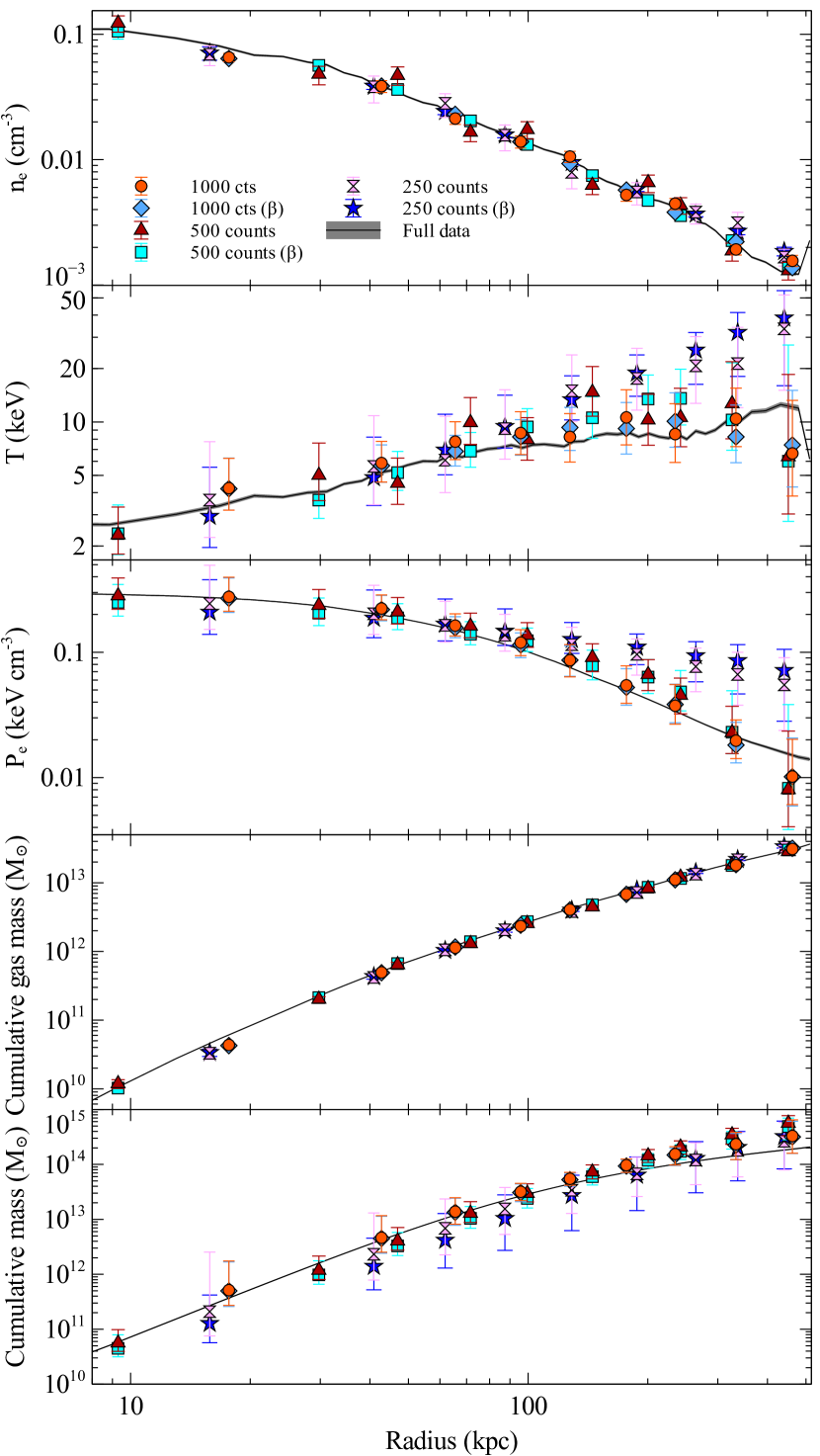
Figure 18: Results from mbproj King model analyses of realisations of PKS0745 surface brightness profiles with short exposure times. Shown are results for clusters with 1000, 500 and 250 counts. For each realisation, we show the results assuming independent densities in each bin and assuming a $\beta$ model.

In this paper we applied the mbproj method to very good quality data. However, the technique can operate in the low count regime, as demonstrated in Fig. 18, which shows results from analysing three realisations of the PKS0745 surface brightness profiles, with 1000, 500 and 250 cluster counts in total. We assume zero background in these simulations. The method is able to reproduce the full density profile and gas mass profile in each case. Reasonable temperature and pressure profiles are obtained with 1000 and 500 count profiles. The total mass profiles are also consistent with the full case, although the uncertainties are large in fractional terms ($\sim 50$ per cent for the 1000 count dataset). In this analysis we assume flat priors on the core radius (between $1\rm\thinspace kpc$ and $2.5\rm\thinspace Mpc$) and on the velocity dispersion (between 10 and $2000\hbox{$\rm\thinspace km\rm\thinspace s^{-1}\,$}$). It is likely that improved priors on the mass model will reduce these uncertainties, although the outer pressure is one of the main uncertainties.

This simple simulation does not include the effects of background or the telescope point spread function (PSF) and only examines a single realisation of a single object, but it shows that the modelling method is likely to be useful in examining data from current and future X-ray cluster surveys (e.g. using eROSITA; Predehl et al. 2010; Merloni et al. 2012). Such a technique would extract the maximum available information from each object and could be a useful improvement over scaling relations. The analysis of better simulations and existing cluster surveys will test the usefulness of the technique for surveys. Indeed, the technique may work better in lower mass objects as it is difficult to measure temperatures using three bands at temperatures of $\sim 10$ keV.

9 Conclusions

We present a new technique, mbproj, for the analysis of thermodynamic cluster profiles without the use of spectral fitting. It assumes hydrostatic equilibrium, spherical symmetry and a dark matter mass model and uses MCMC to deduce the uncertainties on the various thermodynamic quantities. In this cluster, the low obtained gravitational acceleration suggests that the assumptions of hydrostatic equilibrium or spherical symmetry are invalid or that there are additional non-thermal sources of pressure. The code works in the low count regime, suggesting it will be very useful for the analysis of cluster survey data.

The analysis of new Chandra and XMM observations of the PKS0745 galaxy cluster suggest that there is at least a factor of 20 in X-ray gas temperature in this object (from 10 keV to at least 0.5 keV). There is no sharp cut-off in X-ray temperature. It appears, despite the evidence for feedback in the form of central cavities, that cooling of the intracluster medium is occurring at the rate of a few hundred solar masses per year. As found in several other clusters, the coolest material X-ray emitting material and line emitting nebula is offset from the central AGN.

There are two sets of cold front to either side of the nucleus. This could be suggesting sloshing of the gas in the potential well, which would also explain the offset of the coolest material. We investigate the azimuthal variation of projected thermodynamic quantities in the cluster. If the cluster were spherical, we find projected variations of 7 per cent in temperature and pressure and 11 per cent in density. The entropy variation is 13 per cent. If we correct for the shifting isophotes in the cluster, the density variation reduces to 2 per cent and the temperature and entropy variation to 5 and 6 per cent, respectively. Projection effects are likely to increase these by around a factor of 2. The magnitude of the fluctuations depends strongly on how the signal from the underlying cluster is subtracted and so should be considered when comparing to theoretically predicted values.

References

- Allen et al. (1996) Allen S. W., Fabian A. C., Edge A. C., Bautz M. W., Furuzawa A., Tawara Y., 1996, MNRAS, 283, 263
- Allen, Fabian & Kneib (1996) Allen S. W., Fabian A. C., Kneib J. P., 1996, MNRAS, 279, 615
- Allen, Schmidt & Fabian (2001) Allen S. W., Schmidt R. W., Fabian A. C., 2001, MNRAS, 328, L37
- Anders & Grevesse (1989) Anders E., Grevesse N., 1989, Geochim. Cosmochim. Acta, 53, 197
- Arnaud (1996) Arnaud K. A., 1996, in ASP Conf. Ser. 101: Astronomical Data Analysis Software and Systems V, Jacoby G. H., Barnes J., eds., pp. 17–+
- Ascasibar & Markevitch (2006) Ascasibar Y., Markevitch M., 2006, ApJ, 650, 102
- Balucinska-Church & McCammon (1992) Balucinska-Church M., McCammon D., 1992, ApJ, 400, 699
- Baum & O’Dea (1991) Baum S. A., O’Dea C. P., 1991, MNRAS, 250, 737
- Blanton et al. (2011) Blanton E. L., Randall S. W., Clarke T. E., Sarazin C. L., McNamara B. R., Douglass E. M., McDonald M., 2011, ApJ, 737, 99
- Brüggen, Hoeft & Ruszkowski (2005) Brüggen M., Hoeft M., Ruszkowski M., 2005, ApJ, 628, 153
- Canning et al. (2014) Canning R. E. A. et al., 2014, ArXiv e-prints, arXiv:1406.4800
- Cash (1979) Cash W., 1979, ApJ, 228, 939
- Churazov et al. (2012) Churazov E. et al., 2012, MNRAS, 421, 1123
- Crawford et al. (1999) Crawford C. S., Allen S. W., Ebeling H., Edge A. C., Fabian A. C., 1999, MNRAS, 306, 857
- Crawford, Sanders & Fabian (2005) Crawford C. S., Sanders J. S., Fabian A. C., 2005, MNRAS, 361, 17
- de Plaa et al. (2010) de Plaa J., Werner N., Simionescu A., Kaastra J. S., Grange Y. G., Vink J., 2010, A&A, 523, A81
- Donahue et al. (2011) Donahue M., de Messières G. E., O’Connell R. W., Voit G. M., Hoffer A., McNamara B. R., Nulsen P. E. J., 2011, ApJ, 732, 40
- Donahue et al. (2000) Donahue M., Mack J., Voit G. M., Sparks W., Elston R., Maloney P. R., 2000, ApJ, 545, 670
- Durret, Lima Neto & Forman (2005) Durret F., Lima Neto G. B., Forman W., 2005, A&A, 432, 809
- Edge et al. (1990) Edge A. C., Stewart G. C., Fabian A. C., Arnaud K. A., 1990, MNRAS, 245, 559
- Fabian (1994) Fabian A. C., 1994, ARA&A, 32, 277
- Fabian (2012) Fabian A. C., 2012, ARA&A, 50, 455
- Fabian et al. (1985) Fabian A. C. et al., 1985, MNRAS, 216, 923
- Fabian et al. (1981) Fabian A. C., Hu E. M., Cowie L. L., Grindlay J., 1981, ApJ, 248, 47
- Fabian et al. (2003) Fabian A. C., Sanders J. S., Allen S. W., Crawford C. S., Iwasawa K., Johnstone R. M., Schmidt R. W., Taylor G. B., 2003, MNRAS, 344, L43
- Fabian et al. (2011) Fabian A. C., Sanders J. S., Williams R. J. R., Lazarian A., Ferland G. J., Johnstone R. M., 2011, MNRAS, 417, 172
- Foreman-Mackey et al. (2012) Foreman-Mackey D., Hogg D. W., Lang D., Goodman J., 2012, arXiv:1202.3665
- Forman et al. (2007) Forman W. et al., 2007, ApJ, 665, 1057
- Gaspari et al. (2014) Gaspari M., Churazov E., Nagai D., Lau E. T., Zhuravleva I., 2014, ArXiv e-prints, arXiv:1404.5302
- George et al. (2009) George M. R., Fabian A. C., Sanders J. S., Young A. J., Russell H. R., 2009, MNRAS, 395, 657
- Goodman & Weare (2010) Goodman J., Weare J., 2010, Commun. Appl. Math. Comput. Sci., 5, 65
- Hamer et al. (2012) Hamer S. L., Edge A. C., Swinbank A. M., Wilman R. J., Russell H. R., Fabian A. C., Sanders J. S., Salomé P., 2012, MNRAS, 421, 3409
- Heckman et al. (1989) Heckman T. M., Baum S. A., van Breugel W. J. M., McCarthy P., 1989, ApJ, 338, 48
- Heinz, Brüggen & Morsony (2010) Heinz S., Brüggen M., Morsony B., 2010, ApJ, 708, 462
- Hicks & Mushotzky (2005) Hicks A. K., Mushotzky R., 2005, ApJ, 635, L9
- Hicks et al. (2002) Hicks A. K., Wise M. W., Houck J. C., Canizares C. R., 2002, ApJ, 580, 763
- Hlavacek-Larrondo & Fabian (2011) Hlavacek-Larrondo J., Fabian A. C., 2011, MNRAS, 413, 313
- Hoffer et al. (2012) Hoffer A. S., Donahue M., Hicks A., Barthelemy R. S., 2012, ApJS, 199, 23
- Humphrey & Buote (2013) Humphrey P. J., Buote D. A., 2013, MNRAS, 436, 2879
- Johnstone, Fabian & Nulsen (1987) Johnstone R. M., Fabian A. C., Nulsen P. E. J., 1987, MNRAS, 224, 75
- Kalberla et al. (2005) Kalberla P. M. W., Burton W. B., Hartmann D., Arnal E. M., Bajaja E., Morras R., Pöppel W. G. L., 2005, A&A, 440, 775
- King (1962) King I., 1962, AJ, 67, 471
- Lau, Kravtsov & Nagai (2009) Lau E. T., Kravtsov A. V., Nagai D., 2009, ApJ, 705, 1129
- Markevitch & Vikhlinin (2007) Markevitch M., Vikhlinin A., 2007, Phys. Rep., 443, 1
- McDonald et al. (2012) McDonald M. et al., 2012, Nature, 488, 349
- McDonald et al. (2013a) McDonald M., Benson B., Veilleux S., Bautz M. W., Reichardt C. L., 2013a, ApJ, 765, L37
- McDonald et al. (2013b) McDonald M. et al., 2013b, ApJ, 774, 23
- McDonald et al. (2014) McDonald M. et al., 2014, ApJ, 784, 18
- McNamara & Nulsen (2012) McNamara B. R., Nulsen P. E. J., 2012, New Journal of Physics, 14, 055023
- McNamara & O’Connell (1992) McNamara B. R., O’Connell R. W., 1992, ApJ, 393, 579
- Merloni et al. (2012) Merloni A. et al., 2012, ArXiv e-prints, arXiv:1209.3114
- Navarro, Frenk & White (1996) Navarro J. F., Frenk C. S., White S. D. M., 1996, ApJ, 462, 563
- O’Dea et al. (2008) O’Dea C. P. et al., 2008, ApJ, 681, 1035
- O’Sullivan, Vrtilek & Kempner (2005) O’Sullivan E., Vrtilek J. M., Kempner J. C., 2005, ApJ, 624, L77
- Predehl et al. (2010) Predehl P. et al., 2010, in Society of Photo-Optical Instrumentation Engineers (SPIE) Conference Series, Vol. 7732, Society of Photo-Optical Instrumentation Engineers (SPIE) Conference Series
- Roediger et al. (2012) Roediger E., Lovisari L., Dupke R., Ghizzardi S., Brüggen M., Kraft R. P., Machacek M. E., 2012, MNRAS, 420, 3632
- Russell, Sanders & Fabian (2008) Russell H. R., Sanders J. S., Fabian A. C., 2008, MNRAS, 390, 1207
- Salomé & Combes (2003) Salomé P., Combes F., 2003, A&A, 412, 657
- Sanders (2006) Sanders J. S., 2006, MNRAS, 371, 829
- Sanders & Fabian (2007) Sanders J. S., Fabian A. C., 2007, MNRAS, 381, 1381
- Sanders & Fabian (2012) Sanders J. S., Fabian A. C., 2012, MNRAS, 421, 726
- Sanders & Fabian (2013) Sanders J. S., Fabian A. C., 2013, MNRAS, 429, 2727
- Sanders et al. (2008) Sanders J. S., Fabian A. C., Allen S. W., Morris R. G., Graham J., Johnstone R. M., 2008, MNRAS, 385, 1186
- Sanders et al. (2004) Sanders J. S., Fabian A. C., Allen S. W., Schmidt R. W., 2004, MNRAS, 349, 952
- Sanders et al. (2010) Sanders J. S., Fabian A. C., Frank K. A., Peterson J. R., Russell H. R., 2010, MNRAS, 402, 127
- Sanders, Fabian & Taylor (2009a) Sanders J. S., Fabian A. C., Taylor G. B., 2009a, MNRAS, 396, 1449
- Sanders, Fabian & Taylor (2009b) Sanders J. S., Fabian A. C., Taylor G. B., 2009b, MNRAS, 393, 71
- Smith et al. (2001) Smith R. K., Brickhouse N. S., Liedahl D. A., Raymond J. C., 2001, ApJ, 556, L91
- Taylor, Barton & Ge (1994) Taylor G. B., Barton E. J., Ge J., 1994, AJ, 107, 1942
- Taylor, Fabian & Allen (2002) Taylor G. B., Fabian A. C., Allen S. W., 2002, MNRAS, 334, 769
- Vazza et al. (2011) Vazza F., Brunetti G., Gheller C., Brunino R., Brüggen M., 2011, A&A, 529, A17+
- Vazza et al. (2009) Vazza F., Brunetti G., Kritsuk A., Wagner R., Gheller C., Norman M., 2009, A&A, 504, 33
- Wales & Doye (1997) Wales D. J., Doye J. P. K., 1997, J. Phys. Chem. A, 101, 5111
- Walker et al. (2012) Walker S. A., Fabian A. C., Sanders J. S., George M. R., 2012, MNRAS, 3318
- Werner et al. (2014) Werner N. et al., 2014, MNRAS, 439, 2291
- Werner et al. (2010) Werner N. et al., 2010, MNRAS, 407, 2063
- Werner et al. (2011) Werner N. et al., 2011, MNRAS, 415, 3369
- Zhao et al. (1993) Zhao J.-H., Sumi D. M., Burns J. O., Duric N., 1993, ApJ, 416, 51
- Zhuravleva et al. (2014) Zhuravleva I. et al., 2014, ApJ, 788, L13
- ZuHone et al. (2014) ZuHone J. A., Kunz M. W., Markevitch M., Stone J. M., Biffi V., 2014, arXiv:1406.4031