Transition metal solute interactions with point defects in austenitic iron from first principles

Abstract

We present a comprehensive set of first principles electronic structure calculations to study the properties of substitutional transition metal solutes and their interactions with point defects in austenite (face-centred cubic Fe). Clear trends were observed in these quantities across the transition metal series. Solute-defect interactions were found to be strongly correlated to the solute size factors in a manner consistent with local strain field effects. Functional relationships were determined in a number of cases, although for some the early and late transition metal solutes displayed quite distinct behaviour. Strong correlations with results in ferrite (body-centred cubic Fe) were observed throughout, showing insensitivity to the underlying crystal structure in Fe. We confirmed that oversized solutes act as strong traps for both vacancy and self-interstitial defects and as nucleation sites for the development of proto-voids and small self-interstitial loops. The consequential reduction in defect mobility and net defect concentrations in the matrix explains the experimental observation of reduced swelling and radiation-induced segregation in austenitic steels doped with oversized solutes. These results raise the possibility that oversized solutes remaining dissolved in oxide dispersion-strengthened (ODS) steels after manufacturing could contribute to the observed radiation-damage resistance of these materials. Our analysis of vacancy-mediated solute diffusion demonstrates that Ni and Co diffuse more slowly than Fe, along with any vacancy flux produced under irradiation below a critical temperature, which is $400\pm 50$ K for Co and their concentrations should be enhanced at defect sinks. In contrast, Cr and Cu diffuse more quickly than Fe, against a vacancy flux and will be depleted at defect sinks. Oversized solutes early in the transition metal series form highly-stable solute-centred divacancy (SCD) defects with a nearest-neighbour vacancy. The vacancy-mediated diffusion of these solutes is dominated by the dissociation and reassociation of the SCDs, with a lower activation energy than for self-diffusion, which has important implications for the nucleation and growth of complex oxide nanoparticles containing these solutes in ODS steels. Interstitial-mediated solute diffusion is energetically disfavoured for all except the magnetic solutes, namely Cr, Mn, Co and Ni. Given the central role that the solute size factor plays in the results discussed in this work, we would expect them to apply, more generally, to other solvent metals and to austenitic stainless steel alloys in particular.

I Introduction

The addition of major and minor alloying elements to steels has been an essential technique for improving, amongst others things, their mechanical, thermal and chemical properties for a particular application throughout the entire history of iron and steel manufacturing, research and technological progress. In the nuclear industry the push to make the next generation of nuclear fission reactors and prospective fusion reactors as safe and efficient as possible places significant design constraints on the structural materials used to build them. In particular, these materials must be able to withstand higher temperatures, radiation doses and more chemically corrosive environments than previous reactor systems, whilst maintaining their mechanical integrity over timescales of half a century or more.

One of the holy grails in nuclear materials is the so called self-healing material, which exhibits few, if any, of the usual problems found in irradiated materials, such as embrittlement, void formation and swelling, radiation-induced segregation (RIS), irradiation-induced creep (IIC) and irradiation-assisted stress corrosion cracking (IASCC). In the early nineties Kato et al.Kato1991 ; Kato1992 made a significant step in the right direction when they showed that the addition of around 0.35 at.% of oversized transition metal (TM) solutes, such as Ti, V, Zr, Nb, Hf and Ta, to 316L austenitic stainless steel significantly reduced swelling by both prolonging the incubation period for void nucleation to higher doses and suppressing void growth and decreased the RIS of Cr away from and Ni towards grain boundaries usually seen under irradiation. Similar observations were also made by Allen et al.Allen2005 upon adding Zr to Fe-18Cr-9.5Ni austenitic steel. Furthermore, it was observed that these beneficial effects increased in strength with the size-factor of the solute, that is, in the order, Hf$>$Zr$>$Ta$>$Nb$>$Ti$>$VKato1991 ; Kato1992 .

Point defect (and in particular vacancy) trapping at the oversized solutes was suggested as the primary mechanism behind the observationsKato1991 ; Kato1992 , leading to a decrease in defect mobility and net point defect concentrations, either via enhanced recombination or the formation of secondary defects in the matrix. Stepanov et al.Stepanov2004 demonstrated that a model based on the trapping of vacancies by oversized solutes was capable of reproducing the simultaneous suppression of RIS and void swelling observed experimentally. The primary aim of the current work is to improve upon the theoretical understanding of the mechanisms underpinning the experimental observations of Kato et al.Kato1991 ; Kato1992 using detailed first-principle calculations of the atomic-level processes involved.

The incorporation of small oxide nanoparticles, such as Y₂O₃, is another important technique to strengthen and improve the radiation-damage resistance of both ferriticKishimoto2009 ; Hsiung2010 ; Brodrick2014 and austeniticOka2011 ; Oka2013 ; Xu2011 ; Zhou2012 ; Gopejenko steels, allowing them to be used at higher temperatures and radiation dose rates than standard steels. Small quantities of oversized solutes, such as Ti and Hf, are commonly used in the formation of these ODS steels to control the size of the oxide nanoparticles. While it is generally accepted that the mechanical alloying techniques used in the production of these steels fully dissolves the atomic components of the Y₂O₃ and minor alloying element powders into the Fe matrix, the subsequent nucleation and formation of the oxide nanoparticles during heat-treatment and annealing is not completely understood. The possibility for isolated, oversized solutes to remain dissolved in the Fe matrix and contribute to the radiation-damage resistance of ODS steels is also worthy of further investigation. We investigate both of these questions within this work.

To the best of our knowledge, no first-principles calculations have been performed to investigate the general behaviour of TM solutes or their interactions with point defects in austenite. This is directly related to the extensive computational effort required to explicitly model the paramagnetic state of austeniteOlssonB ; Alling ; Kormann12 ; Steneteg and to the large number of near-degenerate reference states capable of modelling metastable austenite at zero KelvinKlaver12 . Density functional theory (DFT) has been used to investigate the properties of Y in austeniteGopejenko , as a first step to understanding Y₂O₃ nanoparticle formation in ODS steel. The non-magnetic (nm) state of face-centred cubic (fcc) Fe was used to model paramagnetic austenite, in contrast to our previous first-principles studies in austeniteKlaver12 ; Hepburn13 ; Ackland11 , where magnetic effects were included explicitly. In this work we have followed a similar methodology by using the face-centred tetragonal (fct), anti-ferromagnetic double-layer (afmD) collinear-magnetic state of Fe to model austeniteKlaver12 ; Hepburn13 ; Ackland11 . We have investigated the properties of TM solutes in this state using first-principles DFT calculations, in a comparable manner to the work of Olsson et al. in the body-centred cubic (bcc) ferromagnetic (fm) Fe ground stateOlsson10 . In particular, we focus on solute interactions with point defects and investigate any general trends across the TM series and possible correlations between these interactions and solute size-factors.

In section II we present the details of our method of calculation. We then proceed to discuss TM solute properties in the defect-free lattice (section III.1) and their interactions with vacancy and self-interstitial defects (in sections III.2 and III.3, respectively) before making our conclusions. A direct and fruitful comparison with results in bcc FeOlsson10 is made throughout. The TM solute data is summarised in Appendix B.

II Computational Details

The calculations have been performed using the plane wave DFT code, VASPKresseHafner ; KresseFurthmuller , in the generalised gradient approximation with exchange and correlation described by the parametrisation of Perdew and WangPW91 and spin interpolation of the correlation potential provided by the improved Vosko-Wilk-Nusair schemevwn . Projector augmented wave (PAW) potentialsBlochl ; KresseJoubert were used for all TM elements. First order Methfessel and Paxton smearingMethfesselPaxton of the Fermi surface was used throughout with a smearing width, $\sigma=0.2$ eV. Spin-polarised (collinear magnetic) calculations have been performed for all magnetic materials with local magnetic moments determined within VASP by integrating the spin density within spheres centred on the atoms. The sphere radii are given in Appendix A.

A set of high-precision calculations were performed to determine the ground state crystallographic and magnetic structures for all the TM elements. A detailed account, including a short review of the significantly more complex structure of Mn, is given in Appendix A, where the results are summarised along with previous results for the fct afmD and fcc nm states of FeKlaver12 . The calculated crystallographic parameters were found to be, typically, within 1-2% of the experimental valuesKittel . Elastic constants for fct afmD Fe were calculated previouslyKlaver12 . Using the same technique, we found that those for fcc nm Fe are $C_{11}=423$ GPa, $C_{12}=217$ GPa, $C_{44}=236$ GPa and the bulk modulus, $B=286$ GPa.

Supercells of 256 ($\pm 1$, $\pm 2$,…) atoms were used for the TM solute calculations with supercell dimensions held fixed at their equilibrium values and ionic positions free to relax. Single configurations were relaxed until the force components were no more than 0.01 eV/$\mathrm{\AA}$. Nudged elastic bandNEB98 (NEB) calculations using a climbing imageHenkelmanClimb00 and improved tangent methodHenkelmanTangent00 were also used to determine migration barriers with a tolerance for energy convergence of 1 meV. A $2^{3}$ k-point Monkhorst-Pack grid was used to sample the Brillouin zone along with a plane wave cutoff energy of 350 eV in all these calculations, which were found to allow formation, binding and migration energies as well as inter-particle separations and local moments to be determined accuratelyKlaver12 .

We model austenite (at $T$=0K) using fct afmD Fe, which is the most stable collinear magnetic reference state structure. This structure consists of ferromagnetically aligned (001) fcc planes of atoms, which we refer to as magnetic planes, with an up,up,down,down double-layer ordering of moments on adjacent planes along the c-direction, as shown in Fig. 1.

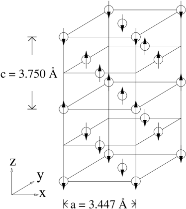
Figure 1: The fct afmD structure of Fe. The arrows indicate the local moments on the atoms, showing the magnetic planes and double-layer magnetic structure. Lattice parameters, $a$ and $c$, are also given.

An important part of this study is a comparison of results in fct afmD Fe with those in bcc fm Fe using data from the work of Olsson et al.Olsson10 . We have performed additional calculations in bcc fm Fe to provide data for the elements Sc, Zn, Y, Cd, Lu and Hg not covered in that study. These calculations were performed in a 128 atom supercell with a greater plane wave cutoff energy of 350 eV, a finer $4^{3}$ Monkhorst-Pack k-point grid and a near-identical lattice parameter to the previous studyOlsson10 [see Appendix A]. A comparison of results for the elements Ti, Cu, Zr, Ag, Hf and Au, between our method and Olsson et al.Olsson10 , showed that formation energies differed by no more than a few hundredths of an eV, which is more than sufficient for our purposes.

We define the formation energy, $E_{\mathrm{f}}$, of a configuration containing $n_{\mathrm{X}}$ atoms of each element, X, relative to a set of reference states for each element using

$$E_{\mathrm{f}}=E-\sum_{\mathrm{X}}n_{\mathrm{X}}E^{\mathrm{ref}}_{\mathrm{X}},$$ (1)

where $E$ is the calculated energy of the configuration and $E^{\mathrm{ref}}_{\mathrm{X}}$ is the reference state energy for element X. We take the reference energies to be the energies per atom in the ground-state crystal structures for all elements except Fe, where the energy per atom in the solvent structure, that is in fct afmD or fcc nm Fe, has been used.

We define the binding energy between a set of $n$ species, $\{A_{i}\}$, where a species can be a defect, solute, clusters of defects and solutes etc., using the indirect method as

$$E_{\mathrm{b}}(A_{1},...,A_{n})=\sum_{i=1}^{n}E_{\mathrm{f}}(A_{i})-E_{\mathrm{f}}(A_{1},...,A_{n})$$ (2)

where $E_{\mathrm{f}}(A_{i})$ is the formation energy for the single species, $A_{i}$, and $E_{\mathrm{f}}(A_{1},...,A_{n})$ is the formation energy for a configuration where the species are interacting. An attractive interaction, therefore, corresponds to a positive binding energy. One intuitive consequence of this definition is that the binding energy of a species, $B$, to an already existing cluster (or complex) of species, $\{A_{1},\dots,A_{n}\}$, which we collectively call $C$, is given by the simple formula,

$$E_{\mathrm{b}}(B,C)=E_{\mathrm{b}}(B,A_{1},\dots,A_{n})-E_{\mathrm{b}}(A_{1},\dots,A_{n}).$$ (3)

This result will be particularly useful when we consider the additional binding of a vacancy or solute to an already existing vacancy-solute complex.

The size factor, $\Omega_{\mathrm{SF}}$, for a substitutional solute, X, in an alloy can be definedStraalsund1974 as the change in volume, $\Delta V$, upon replacing an average alloy atom with an X atom, expressed as a fraction of the average atomic volume per lattice site, $V_{\mathrm{ave.}}$. Practically, it can be defined in terms of the (partial) atomic volume of solute X in the alloy, $V_{\mathrm{X}}$, which is just the change in alloy volume upon adding an atom of solute X to the alloy, or using the concentration (or atomic fraction) of solute X, $c_{\mathrm{X}}$, to yield the following:

$$\Omega_{\mathrm{SF}}=\frac{\Delta V}{V_{\mathrm{ave.}}}=\frac{V_{\mathrm{X}}-V_{\mathrm{ave.}}}{V_{\mathrm{ave.}}}=\frac{1}{V_{\mathrm{ave.}}}\frac{\partial V_{\mathrm{ave.}}}{\partial c_{\mathrm{X}}}.$$ (4)

Our TM calculations use fixed supercells so we have determined $\Omega_{\mathrm{SF}}$ by measuring the pressure, $P$, induced after introducing a single substitutional solute into the pure solvent metal. Any systematic and non-convergence errors in the pressure for these large-cell calculations, which show up as a residual pressure in the pure solvent cell calculation were subtracted in the calculation of $P$. The volume change, $\Delta V$, associated with the introduced solute was calculated by extrapolating to zero pressure using the bulk modulus, $B=-V\mathrm{d}P/\mathrm{d}V$, to give

$$\Delta V=\frac{PV}{B}\ \Rightarrow\ \Omega_{\mathrm{SF}}=\frac{NP}{B}$$ (5)

where $V$ is the cell volume and $N$ is the number of atoms in the cell, which is 256 in this case. The volume extrapolation has an associated energy change, $E^{\mathrm{corr.}}=-P^{2}V/2B$, which, as a result of periodic boundary condition effects, is equal to an Eshelby-type elastic correction for a defect-containing cell embedded in a continuous elastic mediumAcklandA ; HanA . We used this generally applicable result as a measure of the finite-volume error in our calculations and found them to be, generally, negligible compared to other sources of uncertainty.

III Results and Discussion

III.1 TM solutes in the defect-free lattice

We start our investigation of TM solutes in austenite with a study of single substitutional solute properties. We present data for the substitutional (formation) energy, magnetic moment on the substitutional solute and solute size factor across the TM series in Fig. 2. We calculate the substitutional energy relative to the free atom, $E_{\mathrm{f}}^{\mathrm{free}}(\mathrm{sub})$, as well as from the standard reference states, $E_{\mathrm{f}}(\mathrm{sub})$, as in Eq. (1), in order clarify the discussion by removing the bias in the data coming from the varying ground-state crystal structure. Due to the limitations of DFT calculations, we calculate $E_{\mathrm{f}}^{\mathrm{free}}(\mathrm{sub})$ by subtracting the experimental cohesive energy for the ground state crystal structure of the solute element (at 0 K)Kittel [see Appendix A] from $E_{\mathrm{f}}(\mathrm{sub})$. Intuitively, $E_{\mathrm{f}}^{\mathrm{free}}(\mathrm{sub})$, is a generalisation of the (negative) cohesive energy for the pure metals, describing the strength of cohesion of the substitutional solute in the solvent matrix.

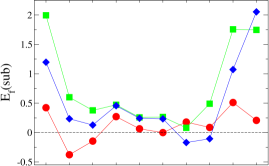
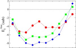
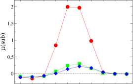
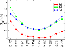
Figure 2: Properties of a single substitutional (sub) solute in fct afmD Fe across the TM series: (a) sub formation energy, $E_{\mathrm{f}}(\mathrm{sub})$, in eV ; (b) sub formation energy relative to the free solute atom, $E_{\mathrm{f}}^{\mathrm{free}}(\mathrm{sub})$, in eV ; (c) local magnetic moment on a sub solute atom when located in a magnetic plane with positive Fe moments, $\mu(\mathrm{sub})$, in $\mu_{\mathrm{B}}$ and (d) solute size factors calculated using the substitutional configuration, $\Omega_{\mathrm{SF}}(\mathrm{sub})$. The data is given in Appendix B.

The substitutional energy curve [Fig. 2] clearly differentiates the majority of the elements, for which $E_{\mathrm{f}}(\mathrm{sub})$ lies below 0.5 eV from those elements at the extremes of the 4d and 5d TM series (groups III, XI and XII), which exhibit substitutional energies up to 2 eV. While no general correlation was observed with the solute size factor, the largest solutes were also the most insoluble. The results also show that Ti, V, Ir and Pt are readily soluble in fct afmD Fe, which is also the case in bcc fm FeOlsson10 .

Changing to a free atom reference state reveals a clear parabolic trend in $E_{\mathrm{f}}^{\mathrm{free}}(\mathrm{sub})$ across the series for the 4d and 5d solutes [Fig. 2]. Such a trend, primarily, results from the filling of the local d band on the solute atom as we proceed across the series, in a similar manner to the Friedel model and its extensions for d band cohesion in the pure transition metalsSutton1993 . Purely atomic processes, such as the energy needed to promote the solute atom from its electronic ground state to that found in the metal and the loss of the atomic magnetic moment and the associated exchange energyBrooks1983 do, however, act to reduce this cohesion. This effect is greatest for those atoms having a half-filled d shell and the largest atomic moments, leading to the observed flattening of the curve near the centre of the series. While the 3d solute data also exhibits a parabolic trend early and late in the series, competition between these atomic processes and a lower d band cohesion than found for the 4d and 5d solutes leads to a pronounced reduction in solute cohesion near the centre of the series. The competition is sufficiently strong that the elements showing the greatest deviation from the parabolic trend, namely Cr, Mn, Fe and Co, maintain part of their atomic moment, as can be seen in Fig. 2.

For all the other TMs, which aside from Ni have non-magnetic ground state crystal structures, the local magnetic order in fct afmD Fe induces small moments on the solutes. The trend in moments is similar to that observed in bcc fm FeOlsson10 , despite the differences in local magnetic ordering, although the moments are much larger there. The case of Cr is particularly interesting as it is well known to be antiferromagnetically aligned in bcc fm FeOlsson10 but shows positive alignment to its magnetic plane in fct afmD Fe. We note, however, that the nearest Fe atoms to a Cr solute in fct afmD Fe actually lie in the adjacent and anti-aligned magnetic plane to the one the solute is embedded in and not in the plane itself, as is the case with all the other TM solutes. We postulate that the earlier shift from anti-alignment to alignment, and the much smaller magnitude moments observed in fct afmD Fe compared to bcc fm Fe, result directly from the competing influence of these oppositely aligned 1nn Fe atoms on the solute moment.

The size factor data [in Fig. 2] exhibits a clear, functional dependence on local d band occupancy, much as was found in bcc FeOlsson10 . The solute size is greatest for early and late elements in the TM series and generally increases down a group, although the lanthanide contraction (resulting from the weak screening provided by the 4f shell) results in 4d and 5d solutes having similar sizes. Size factors for a number of TM solutes have been measured experimentally in 316L austenitic stainless steelStraalsund1974 ; Kato1991 , which has an approximate composition of Fe-17Cr-13Ni (in wt%). We have extrapolated these results to the case of pure Fe by assuming a fixed value for the (partial) atomic volume of Fe atoms and compare to our work in Table 1. For comparison, we also include results for the interstitial solutes C and N from our previous workHepburn13 .

Data	316L	316L	316L steel	This
Set	steelStraalsund1974	steelKato1991	extrapolated	work
$V_{\mathrm{ave.}}$	11.64	11.60	11.43	11.14
$\Omega_{\mathrm{SF}}$(Ti)	—	0.373	0.393	0.457
$\Omega_{\mathrm{SF}}$(V)	—	0.100	0.116	0.188
$\Omega_{\mathrm{SF}}$(Cr)	0.048	—	0.068	0.070
$\Omega_{\mathrm{SF}}$(Mn)	0.034	—	0.054	0.063
$\Omega_{\mathrm{SF}}$(Co)	-0.065	—	-0.047	0.009
$\Omega_{\mathrm{SF}}$(Ni)	-0.032	—	-0.014	0.056
$\Omega_{\mathrm{SF}}$(Cu)	0.093	—	0.114	0.221
$\Omega_{\mathrm{SF}}$(Zr)	—	1.562	1.600	1.180
$\Omega_{\mathrm{SF}}$(Nb)	—	0.625	0.649	0.803
$\Omega_{\mathrm{SF}}$(Mo)	0.359	—	0.384	0.563
$\Omega_{\mathrm{SF}}$(Hf)	—	1.931	1.975	1.027
$\Omega_{\mathrm{SF}}$(Ta)	—	0.786	0.813	0.745
$\Omega_{\mathrm{SF}}$(C)	0.539	—	0.549	0.529
$\Omega_{\mathrm{SF}}$(N)	0.451	—	0.460	0.537

Table 1: Comparison between the average atomic volume per lattice site, $V_{\mathrm{ave.}}$, in $\mathrm{\AA}^{3}$ and size factor, $\Omega_{\mathrm{SF}}$, data from this work and from experimental studies of 316L austenitic stainless steelKato1991 ; Straalsund1974 . The results for C and N from our previous workHepburn13 are also given. The experimental results have been extrapolated to the case of pure Fe by assuming a fixed value for the (partial) atomic volume of Fe atoms.

Our calculation of the atomic volume in austenite is in good agreement with the extrapolated experimental value, although as in bcc FeOlsson10 the DFT method used underestimates it by around 3%. There is also a reasonable agreement between the size factor data but with a general tendency of our results to overestimate the experimental values. The underestimation of $V_{\mathrm{ave.}}$ is certainly a contributing factor, although the finite experimental temperature and the error associated with the extrapolation to pure Fe will also contribute. For the largest solutes (Zr and Hf), however, our results significantly underestimate the size factors. Kato et al.Kato1991 do, however, admit that the size factor of Hf may well be overestimated, and the uncertainties are greatest in their data for Hf and Zr. This may also help explain the different order of 4d and 5d solute sizes we find compared to experimentKato1991 . While we do agree that the group IV TMs are larger than those in group V we find that the 4d solutes are larger than the 5d (that is Zr$>$Hf$>$Nb$>$Ta), in contrast to Kato et al. (where Hf$>$Zr$>$Ta$>$Nb) but consistent with the relative order of atomic volumes in the pure ground state crystal structures and with results in bcc FeOlsson10 . Despite these discrepancies, the generally good agreement between our results and experiment, particularly in the reproduction of the general trend across the TM series, gives us further confidence in our theoretical approach to modelling austeniteKlaver12 ; Hepburn13 .

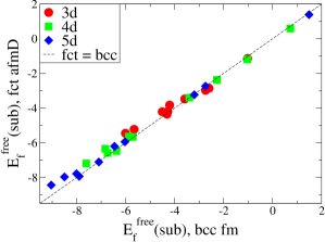
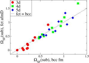
Figure 3: Comparison of (a) the substitutional formation energies relative to the free atom, $E_{\mathrm{f}}^{\mathrm{free}}(\mathrm{sub})$, in eV and (b) the solute size factors, $\Omega_{\mathrm{SF}}(\mathrm{sub})$, between fct afmD Fe and bcc fm FeOlsson10 . The data is given in Appendix B.

We have already observed a number of similarities between our results in fct afmD Fe and those in bcc fm FeOlsson10 . Following the finding of strong correlation between results in pure Fe between these two states by Klaver et al.Klaver12 , we further compare the properties of substitutional TM solutes in the two states. Fig. 3 demonstrates the high level of correlation present in the $E_{\mathrm{f}}^{\mathrm{free}}(\mathrm{sub})$ and $\Omega_{\mathrm{SF}}(\mathrm{sub})$ data between these two states of Fe. That said, there is a slight tendency for solutes in the fct afmD state to exhibit greater cohesion. Overall, these results add to the set of measurable defect and solute properties in Fe that show a marked insensitivity to the details of the surrounding crystal structure.

III.2 TM Solute interactions with vacancy defects

We now turn to investigate the interactions of TM solutes with vacancies in fct afmD Fe.

III.2.1 Vacancy-solute binding

The binding energies between a vacancy and TM solute, X, at 1nn separation, $E_{\mathrm{b}}(\mathrm{vac,X;1nn})$, are shown in Fig. 4. In fct afmD Fe, there are three distinct 1nn configurations, labelled 1a, 1b and 1c in Fig. 5, and the error bars in the plots mark the spread in binding energies with the data points chosen at the centre of the range.

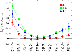
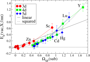
Figure 4: Vacancy-solute binding energies at 1nn, $E_{\mathrm{b}}(\mathrm{vac,X;1nn})$, in eV (a) across the TM series and (b) versus the solute size factor, $\Omega_{\mathrm{SF}}(\mathrm{sub})$, in fct afmD Fe. The error bars identify the spread in binding energies over the three distinct 1nn sites, namely 1a, 1b and 1c in Fig. 5, with the data point chosen at the centre of this range. Figure (b) also shows the results of fits to the combined dataset using a linear, $E_{\mathrm{b}}=0.49\ \Omega_{\mathrm{SF}}$, or squared, $E_{\mathrm{b}}=0.47\ {\Omega_{\mathrm{SF}}}^{2}$, functional dependence. The data is given in Appendix B.

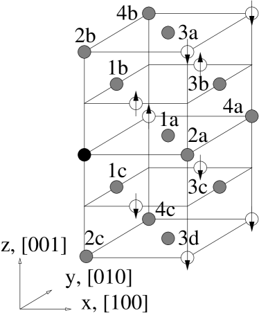
Figure 5: Distinct configurations for an interacting point-defect (black) and substitutional solute (grey) in fct afmD Fe at up to 4nn separation. Fe atoms (white) are shown with arrows to indicate the local moments within their magnetic planes, which are also shown.

The data follows a clear trend across the TM series with all elements, aside from Cr and Mn, being attracted to the vacancy and those early and late in the series showing the strongest binding. Experimental estimatesKato1991 of the binding energies for Ti (0.14 eV) and Nb (0.18 eV) in 316L steel are consistent with our data. The similarity of the trend in the binding energy data to that for the solute size factors [in Fig. 2] is borne out in Fig. 4, which demonstrates a strong correlation between these two quantities, although with a slight tendency for early TMs to interact more strongly than those late in the series, as observed in bcc FeOlsson10 . A linear fit to the data, with a proportionality coefficient of 0.49 eV, is close to the value of 0.45 eV found in bcc FeOlsson10 . A function proportional to the square of the size factor, which could be motivated from elasticity arguments, does, however, give better agreement with the data. Overall, these results confirm the suggestions from experimentKato1991 ; Kato1992 and theoryStepanov2004 that oversized solutes act as trapping sites for vacancies.

What is not apparent from Fig. 4 is that the largest solutes, namely Sc, Y, Zr, Lu and Hf, relax to exactly half way between their original lattice site and the vacancy at 1nn, that is to the centre of the associated divacancy, forming what we refer to as a solute-centred divacancy (SCD). All other solutes remain on-site during relaxation. This behaviour was already observed for He in austeniteHepburn13 and for the same TM solutes in bcc FeOlsson10 and clearly has important implications for vacancy-mediated solute diffusion, which we now discuss.

III.2.2 Vacancy-mediated solute diffusion

The vacancy-mediated diffusion of a substitutional solute in an fcc lattice is usually well described by the five-frequency model of Lidiard and LeClaireLidiard55 ; LeClaire56 . The distinct types of vacancy jumps, as labelled by their associated frequencies, $\omega_{i}$, are given in Fig. 6.

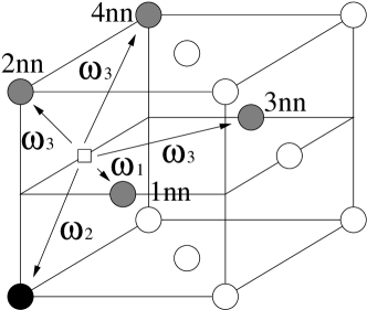
Figure 6: The distinct types of vacancy (white square) jumps near a substitutional solute (black circle) in the fcc lattice for the five-frequency model of Lidiard and LeClaireLidiard55 ; LeClaire56 . Solvent metal atoms involved in the vacancy jumps (grey circles) are distinguished from those in the background matrix (white circles). With the vacancy initially at 1nn to the solute the jumps can either maintain a 1nn separation ($\omega_{1}$), have the vacancy exchange with the solute ($\omega_{2}$) or involve dissociation to ($\omega_{3}$) or association from ($\omega_{4}$) 2nn, 3nn and 4nn separation. In the model, all other vacancy jumps are considered identical to that in the pure solvent metal ($\omega_{0}$).

The frequencies are related to migration barriers by Arrhenius-type expressions,

$$\omega_{i}=C_{\mathrm{m},i}\exp(-\beta E_{\mathrm{m}}(\omega_{i})),$$ (6)

where $\beta=1/k_{\mathrm{B}}T$ and $E_{\mathrm{m}}(\omega_{i})$ is the migration energy for the jump. For vacancies in an fcc lattice, the single maximum in energy along the jump path [see Fig. 7] defines the transition state (TS) and $E_{\mathrm{m}}(\omega_{i})$ is, therefore, the energy difference between the TS and the initial jump configuration. A nearby solute, X, can change the energy of both of these configurations (relative to a non-interacting state). For the initial configuration, I, this is quantified by the vacancy binding energy, $E_{\mathrm{b}}(\mathrm{vac,X;I})$, and we can, similarly, define a “binding energy to the transition state”, $E_{\mathrm{b}}(\mathrm{TS,X};\omega_{i})$. The change in migration energy relative to that in pure Fe is then given by

$$E_{\mathrm{m}}(\omega_{i})=E_{\mathrm{m}}(\omega_{0})+E_{\mathrm{b}}(\mathrm{vac,X;I})-E_{\mathrm{b}}(\mathrm{TS,X};\omega_{i}).$$ (7)

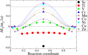
Figure 7: Change in formation energy, $\Delta E_{\mathrm{f}}(\omega_{2},\mathrm{1a})$, in eV, for the 3d TM solutes in fct afmD Fe along the 1a jump path for vacancy-solute exchange [see Fig. 5]. The zero of energy corresponds to a non-interacting vacancy and substitutional solute. The reaction coordinate is the solute position, after rescaling, with 0 or 1 corresponding to a perfectly on-site solute and 0.5 to the case where it is half-way between the two lattice sites, that is to the SCD. The higher dotted line gives the vacancy migration energy for this jump path in pure fct afmD Fe.

We first investigate vacancy-solute exchange, that is jump $\omega_{2}$, for which there are three distinct paths in fct afmD Fe [see Fig. 5], namely 1a, 1b and 1c. Fig. 7 shows the change in formation energy along the 1a jump path, $\Delta E_{\mathrm{f}}(\omega_{2},\mathrm{1a})$, for the 3d solutes. All solutes relax towards a vacancy at 1nn, with larger solutes relaxing further, and Sc going to the symmetric position to form a stable SCD configuration, which is the TS for the other solutes. While the increasing vacancy binding energy leads to a steady lowering of the initial on-site energy, the TS binding energy increases more quickly with size factor, leading to a net lowering of the migration barrier, which is ultimately responsible for the formation of the stable SCD for Sc. Similar results were found for the other migration paths and TM solutes, with Sc, Y, Lu, Zr and Hf forming stable SCDs.

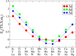
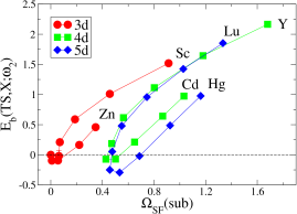
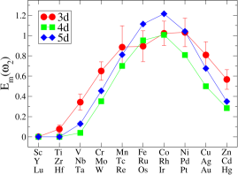
Figure 8: Migration energies, $E_{\mathrm{m}}(\omega_{2})$, and binding energies to the transition state, $E_{\mathrm{b}}(\mathrm{TS,X};\omega_{2})$, in eV for vacancy-solute exchange in fct afmD Fe. The error bars for the 3d solutes and for Y, Zr, Lu and Hf show the spread in energies over the 1a and 1b jump paths [see Fig. 5] with the data point taken as the mean value. The data for path 1c was deemed unreliable given that the magnetic moment on the migrating atom is constrained to be zero in the transition state, leading to an overestimation of the migration energyKlaver12 . Systematic cancellations have resulted in the error bars being smaller than the symbols in figures (a) and (b). For the other solutes only the 1a jump data is shown. The data is given in Appendix B.

Fig. 8 shows $E_{\mathrm{m}}(\omega_{2})$ and $E_{\mathrm{b}}(\mathrm{TS,X};\omega_{2})$ across the TM series. The TS binding energy trend shows strong positive binding at the beginning and end of the series. While there is no simple relationship between solute size and TS binding [Fig. 8], in contrast to the vacancy binding [Fig. 4], the two are still strongly correlated. Generally, the TS binding energy grows at a greater rate than the vacancy binding energy with size factor, which Eq. (7) shows leads to an overall reduction in $E_{\mathrm{m}}(\omega_{2})$ as we move out from the centre of the TS series [Fig. 8]. The extreme examples are Sc, Y, Zr, Lu and Hf, where the energy barrier ceases to exist and the SCD is stable. The barrier heights for Ti, Nb and Ta are also effectively negligible [see Fig. 7 for Ti] and should be considered as forming stable SCDs at finite temperature. Near the centre of the series, by contrast, a combination of positive binding to the vacancy and negative binding to the transition state (see Os and Ir in particular) leads to greater migration energies than in pure Fe. It is also interesting to note that the significant difference between the $\omega_{2}$ jumps for Cr and Ni found previouslyKlaver12 , predominantly result from differences in binding to the transition state (instead of the vacancy), which results, most likely, from magnetic interactions, given the similar solute sizes.

We also investigated the relative importance of vacancy-solute exchange at 2nn to vacancy-mediated diffusion using Y in fct afmD Fe. This was motivated by results from our previous work on substitutional HeHepburn13 . While the TS binding energy for Y along the 2a jump path [see Fig. 5] was significant at 1.82 eV, it was only sufficient to reduce the migration energy to 1.74 eV. Using the data for $\omega_{2}$ jumps as a reference [see Fig. 8] we would expect the migration barriers for the other TM solutes to be in excess of the Y value and can, therefore, conclude that vacancy-solute exchange at 2nn is unlikely to contribute significantly to their vacancy-mediated diffusion.

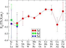
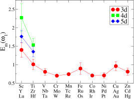
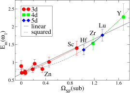
Figure 9: Migration energies, $E_{\mathrm{m}}(\omega_{1})$, and binding energies to the transition state, $E_{\mathrm{b}}(\mathrm{TS,X};\omega_{1})$, in eV for $\omega_{1}$ jumps in fct afmD Fe. For all solutes except Y we have considered the jumps from 1b to 1b and from 1c to 1c configurations [see Figs. 5 and 6], which have symmetry-stabilised transition states, and the error bars reflect the spread in these values. For the special case of Y the 1a to 1b jump, which required the use of climbing image NEB calculations, was also included. The 1a to 1c jump was excluded from the analysis given that the constraints of collinear spin calculations would lead to a zero moment on the migrating Fe atom at some point on the path, resulting in a significant overestimation of the migration energy. Figure (c) also shows the results of linear, $E_{\mathrm{m}}=0.68+0.81\ \Omega_{\mathrm{SF}}$, or squared, $E_{\mathrm{m}}=0.80+0.54\ {\Omega_{\mathrm{SF}}}^{2}$, fits to the combined data. The data is given in Appendix B.

For the $\omega_{1}$ jumps, we have focussed on the 3d solutes and those that form stable SCDs, namely Y, Zr, Lu and Hf. The results are presented in Fig. 9. While the dependence on details of local magnetic state for some elements is large, the TS binding energy is, generally, negative and much smaller than either the $\omega_{2}$ TS or 1nn vacancy binding energies. Both the trend in the $E_{\mathrm{m}}(\omega_{1})$ data [Fig. 9] and its correlation with the size factor [Fig. 9], therefore, primarily result from the vacancy-solute binding energy data [Fig. 4]. The intuitive result is that the migration energy for an $\omega_{1}$ jump increases with solute size factor and the data in Fig. 9 is well described by a linear or quadratic fit function.

In previous analysis of Ni and CrKlaver12 , the ratio of the tracer diffusion coefficient for solute X to that for the solvent, $D^{*}_{\mathrm{X}}/D^{*}_{\mathrm{Fe}}$, and the vacancy wind parameter, $G$, which measures the relative orientations of the solute and vacancy fluxes, were found to be controlled by only two parameters, namely $E_{\mathrm{b}}(\mathrm{TS,X};\omega_{1})$ and $E_{\mathrm{b}}(\mathrm{TS,X};\omega_{2})$. By using the fact that $D^{*}_{\mathrm{X}}/D^{*}_{\mathrm{Fe}}$ is a monotonically increasing function of both parameters and $G$ is a monotonically decreasing function of $E_{\mathrm{b}}(\mathrm{TS,X};\omega_{1})$, we have plotted lower and upper bounds for these quantities for Cr, Mn, Co, Ni and Cu in Fig. 10 using the parameter values and their uncertainties in Table 2.

Element	$E_{\mathrm{b}}(\mathrm{TS,X};\omega_{1})$	$E_{\mathrm{b}}(\mathrm{TS,X};\omega_{2})$
Cr	$-0.042\pm 0.022$	$0.210\pm 0.022$
Mn	$-0.066\pm 0.000$	$-0.019\pm 0.092$
Co	$0.061\pm 0.007$	$-0.097\pm 0.040$
Ni	$0.056\pm 0.065$	$-0.094\pm 0.003$
Cu	$-0.166\pm 0.103$	$0.164\pm 0.022$

Table 2: Binding energies to the transition state for $\omega_{1}$ and $\omega_{2}$ jumps, in eV. The errors and central values are as described in Figs. 8 and 9.

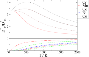
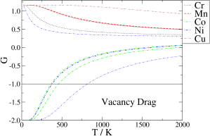
Figure 10: Temperature dependence of (a) the tracer diffusion coefficient ratio, $D^{*}_{\mathrm{X}}/D^{*}_{\mathrm{Fe}}$, and (b) the vacancy wind parameter, $G$, for the solutes Cr (black, dotted line), Mn (red, dashed line), Co (green, dot-dashed line), Ni (blue, double-dot-dashed line) and Cu(brown, dot-double-dashed line). The lower and upper curves for each element show the likely uncertainties. The third, bolder, central curves for Mn in figure (a) and Ni in figure (b) correspond to the central parameter values in Table 2. The vacancy drag regime ($G<-1$) is identified in figure (b).

We find that Ni and Co diffuse at a similar rate and more slowly than Fe, primarily as a result of their negative binding to the $\omega_{2}$ transition state. In contrast, both Cu and Cr exhibit positive TS binding and diffuse more quickly than Fe. For Mn, $E_{\mathrm{b}}(\mathrm{TS,X};\omega_{2})$ spans both positive and negative values, leading to uncertainty in $D^{*}_{\mathrm{X}}/D^{*}_{\mathrm{Fe}}$. The data does, however, show that Mn will diffuse more slowly than either Cr or Cu. In addition to this analysis of diffusion rates, the vacancy wind parameter, $G$, allows one to determine whether the solute flux induced by vacancy-mediated diffusion would be in the same direction (for $G<-1$) or opposite to (for $G>-1$) any vacancy flux. The net diffusion of Cr, Mn and Cu is opposite to the vacancy flux at all temperatures [Fig. 10]. While the behaviour of Ni does appear poorly determined, this results from the $E_{\mathrm{b}}(\mathrm{TS,X};\omega_{1})$ parameter extending to the small but negative value of -0.009 eV at its lower bound, leading to the divergent behaviour seen between the upper and two lower curves for $G$. A positive value is much more likely, meaning that the Ni flux flips from being opposite to the vacancy flux to being in the same direction below a critical temperature, $T_{\mathrm{c}}$, where radiation-induced vacancies drag the solutes with them to the defect sinks. We estimate a value of $T_{\mathrm{c}}=400\pm 50$ K for Co. Overall, these observations are consistent with the RIS of Cr away from and Ni towards vacancy sinks in austenitic stainless steelsKato1991 ; Kato1992 ; Allen2005 . Furthermore, they suggest that Co concentrations will be enhanced and Cu depleted from vacancy sinks. The behaviour of Mn remains undetermined in this study as it depends critically on whether it diffuses faster or slower than Fe, leading, respectively, to depletion or enhancement at defect sinks.

Another useful area of approximation is the case where the $\omega_{2}$ jump frequency becomes very much greater than both $\omega_{1}$ and $\omega_{3}$. This approximation not only applies when $E_{\mathrm{m}}(\omega_{2})$ is small, as is the case for many oversized solutes, but also allows us to treat the case when the migration barrier ceases to exist and a stable SCD is formed. In this limit the general expression for $D^{*}_{\mathrm{X}}$ [see Klaver et al.Klaver12 ] becomes independent of $\omega_{2}$ and is given by,

$$D^{*}_{\mathrm{X}}=a^{2}c_{\mathrm{V}}C_{\mathrm{b}}\exp(\beta E_{\mathrm{b}}(\mathrm{vac,X;1nn}))\left[\omega_{1}+\frac{7}{2}F(\frac{\omega_{4}}{\omega_{0}})\omega_{3}\right],$$ (8)

where $a$ is the fcc lattice parameter, $c_{\mathrm{V}}$, is the vacancy concentration, $C_{\mathrm{b}}$ is a weakly temperature-dependent prefactor that depends on the vacancy-solute binding entropy and the function, F, gives the fraction of dissociative ($\omega_{3}$) jumps that do not effectively return the vacancy to its original siteManning .

The physical interpretation of the large $\omega_{2}$ limit is that the solute oscillates rapidly over a small $\omega_{2}$ barrier or is located about the centre of the associated divacancy, until an $\omega_{1}$ or $\omega_{3}$ jump takes place. $\omega_{1}$ corresponds to the migration of the (effective) SCD as a single entity, which we investigated as a primary mechanism for substitutional He diffusion previouslyHepburn13 . $\omega_{3}$ corresponds to the net diffusion resulting from dissociation (and reassociation) events. The activation energy for both of these diffusion mechanisms is given by

$$E_{\mathrm{A}}(\omega_{i}) = E_{\mathrm{m}}(\omega_{i})-E_{\mathrm{b}}(\mathrm{vac,X;1nn})\ \left[\ +E_{\mathrm{f}}(\mathrm{vac})\ \right]$$ (9)

$$= E_{\mathrm{m}}(\omega_{0})-E_{\mathrm{b}}(\mathrm{TS,X};\omega_{i})\ \left[\ +E_{\mathrm{f}}(\mathrm{vac})\ \right],$$

where the vacancy formation energy, $E_{\mathrm{f}}(\mathrm{vac})$, is either present for a thermal vacancy population or absent for a fixed supersaturation of vacancies, as found in irradiated materials, and the tracer diffusion coefficient remains proportional to the vacancy concentration. Eq. (9) shows that $E_{\mathrm{A}}(\omega_{i})$ is lower than the activation energy for (tracer) self-diffusion by the TS binding energy, $E_{\mathrm{b}}(\mathrm{TS,X};\omega_{i})$. We note, in passing, that while we did not consider the $\omega_{3}$ diffusion mechanism for substitutional He previouslyHepburn13 , test calculations showed it should exhibit a similar TS binding and activation energy to the $\omega_{1}$ mechanism.

For the TS solutes the $E_{\mathrm{b}}(\mathrm{TS,X};\omega_{1})$ data in Fig. 9 suggests that the activation energy for the $\omega_{1}$ diffusion mechanism will, generally, be higher than for self-diffusion. A general study of $\omega_{3}$ (and $\omega_{4}$) jumps would have been prohibitively expensive, given the requirement of 10 relaxed configuration calculations and 9 NEB calculations per solute. We have, however, completed this study for Y, both as the largest solute and for its importance in ODS steels. The results are summarised in Table 3 along with suitably-averaged effective values for the $\omega_{3}$ and $\omega_{4}$ jump data following the method of Tucker et al.Tucker10 .

	$E_{\mathrm{m}}(\omega_{i})$	$E_{\mathrm{b}}(\mathrm{vac,X;I})$	$E_{\mathrm{b}}(\mathrm{TS,X};\omega_{i})$
$\omega_{0}$	$0.90\pm 0.15$	0	0
$\omega_{1}$	$2.27\pm 0.37$	$1.27\pm 0.12$	$-0.10\pm 0.24$
$\omega_{2}$	0	$1.27\pm 0.12$	$2.16\pm 0.03$
$\omega_{3}$, 2nn	$1.97\pm 0.16$	$1.27\pm 0.12$	$0.28\pm 0.22$
$\omega_{3}$, 3nn	$1.43\pm 0.23$	$1.27\pm 0.12$	$0.65\pm 0.20$
$\omega_{3}$, 4nn	$1.31\pm 0.05$	$1.27\pm 0.12$	$0.93\pm 0.05$
$\omega_{3}$, eff	$1.40\pm 0.20$		$0.76\pm 0.23$
$\omega_{4}$, 2nn	$0.59\pm 0.28$	$-0.13\pm 0.03$	$0.28\pm 0.22$
$\omega_{4}$, 3nn	$0.20\pm 0.12$	$0.09\pm 0.08$	$0.65\pm 0.20$
$\omega_{4}$, 4nn	$0.13\pm 0.04$	$0.15\pm 0.07$	$0.93\pm 0.05$
$\omega_{4}$, eff	$0.20\pm 0.12$		$0.76\pm 0.23$

Table 3: Migration energy, $E_{\mathrm{m}}(\omega_{i})$, and solute binding energies to the vacancy in the initial jump configuration, $E_{\mathrm{b}}(\mathrm{vac,X;I})$, and the transition state, $E_{\mathrm{b}}(\mathrm{TS,X};\omega_{i})$, in eV for vacancy jumps near a Y solute in fct afmD Fe. The distinct jumps are given in Fig. 6. Note that there is only one transition state for corresponding $\omega_{3}$ and $\omega_{4}$ jumps so the binding energies are identical. The errors give the spread in energies over the distinct $\omega_{i}$ jump paths in fct afmD Fe or initial configurations [see Fig. 5] with the given value chosen at the centre of this range. The data is given in Appendix B. The effective (eff) $\omega_{3}$ and $\omega_{4}$ migration barriers (and TS binding energies) were calculated from those for 2nn, 3nn and 4nn jumps following the method of Tucker et al.Tucker10 and are valid in a temperature range from 0 to 2000 K.

The vacancy binding energy data exhibits a clear trend of strong attraction at 1nn followed by a much weaker repulsive interaction at 2nn and weak attraction at 3nn and 4nn separations. The same trend was reported in fcc nm FeGopejenko , although with a discrepancy in binding energy of up to 0.4 eV. We put this discrepancy down to their choice of much smaller (96 atom) supercells rather than the difference in magnetic reference state, given that our own (256 atom cell) calculations in fcc nm Fe found binding energies at the centres of the ranges reported in Table 3. It is interesting to note that a very similar trend was also observed for early TM solutes in bcc FeOlsson10 and for He in austeniteHepburn13 . In contrast to the rather sharp fall-off in vacancy binding, the binding energies to the $\omega_{3}$ (and $\omega_{4}$) transition states remain high at as much as 1 eV. This translates into much lower migration energies than for $\omega_{1}$ jumps and the $\omega_{3}$ mechanism will, therefore, dominate the vacancy-mediated diffusion of Y solutes. While the $\omega_{3}$ migration energies remain greater than in pure Fe, the high TS binding energies mean that the corresponding activation energies [Eq. (9)] are much lower than for self-diffusion. This result means that Y will diffuse faster than Fe above some critical temperature, despite its much greater size. Another important consequence of the strong TS binding energies are the very low migration energies for $\omega_{4}$ jumps, with an effective value of $0.20\pm 0.12$ eV, which is significantly less than in pure Fe. Such a low value means that a newly dissociated vacancy is much more likely to return to the solute than be lost to the general matrix (making an $\omega_{0}$ jump) and it is reasonable to ask why this does not significantly suppress diffusion through the factor, $F(\omega_{4}/\omega_{0})$ in Eq. (8). However, even in the limit where the vacancy always returns, that is $\omega_{4}/\omega_{0}\rightarrow+\infty$, $F$ remains above zero at $2/7$. This results from the fact that the vacancy can return to different sites at 1nn to the solute from the one it left and, therefore, still contribute to diffusionManning .

Thus we can state with reasonable confidence that the $\omega_{3}$ diffusion mechanism will dominate for the early (oversized) TM solutes with an activation energy lower than that for self-diffusion. The enhanced mobility of these solutes is, certainly, an important factor in understanding the nucleation and formation of the complex oxide nanoparticles produced during the manufacturing of ODS steels, although other factors, such as oxygen mobility and the interactions between the oxide components will also be importantGopejenko .

III.2.3 Vacancy clustering and void nucleation

In the experimental work of Kato et al.Kato1991 it was shown that, while the addition of oversized TM solutes to 316L steel did suppress void growth and reduce void swelling under irradiation, this was accompanied by an abrupt increase in void number density above a certain solute size factor and for sufficiently-high radiation doses. On this basis, the authors suggested that the oversized solutes were acting as void nucleation sites. We have investigated this possibility by studying the growth of vacancy clusters around a single Y atom, that is vac_n-Y clusters, and the binding energies for the most stable clusters are given in Table 4.

$n$	1	2	3	4	5
$E_{\mathrm{b}}^{\mathrm{tot}}$	$1.27\pm 0.12$	$3.12\pm 0.01$	$5.11\pm 0.02$	5.06	6.51
$E_{\mathrm{b}}^{\mathrm{vac}}$	$1.27\pm 0.12$	$1.85\pm 0.14$	$1.99\pm 0.03$	$-0.05\pm 0.02$	1.46
$E_{\mathrm{b}}^{\mathrm{Y}}$	$1.27\pm 0.12$	$3.02\pm 0.08$	$4.50\pm 0.05$	$4.06\pm 0.29$	4.83

Table 4: The total binding energy between $n$ vacancies and a substitutional Y solute in a vac_n-Y cluster, $E_{\mathrm{b}}^{\mathrm{tot}}$, the binding energy for adding a vacancy to a vac_n-1-Y cluster, $E_{\mathrm{b}}^{\mathrm{vac}}$, and the binding energy of a substitutional Y solute to a vac_n cluster, $E_{\mathrm{b}}^{\mathrm{Y}}$, in eV for the most stable clusters in fct afmD Fe. The difference between $E_{\mathrm{b}}^{\mathrm{tot}}$ and $E_{\mathrm{b}}^{\mathrm{Y}}$ is, therefore, the total binding energy of the most stable vac_n cluster. The errors give the spread in binding energies over the distinct configurations in fct afmD Fe that would be equivalent in austenite with the data point taken at the centre of this range. For $n=4$, only the most stable configuration was used and for $n=5$ the most stable cluster is uniquely defined in fct afmD Fe.

A single vacancy binds strongly at 1nn to a Y solute, forming a stable SCD, as discussed previously. Once formed, an SCD acts as an even stronger trap for vacancies than the Y solute alone. A second vacancy binds to the SCD to form a close-packed triangle of vacancies lying in a (111) plane with the Y atom at the centre. The corresponding configuration in pure fct afmD Fe was found to be unstable, suggesting that the configuration is only stable for solutes above a critical size, as observed for the SCD. The pattern continues with the addition of a third vacancy, which binds to form a tetrahedron of vacancies, mutually at 1nn separation, with the Y atom, once again, relaxing to the centre of this proto-void. This type of configuration, which in pure fcc metals is know as the Damask-Dienes-Weizer (DDW) structureDamask1959 and is the smallest possible stacking fault tetrahedronVineyard1961 there, was also found to be the most stable trivacancy cluster in austeniteKlaver12 .

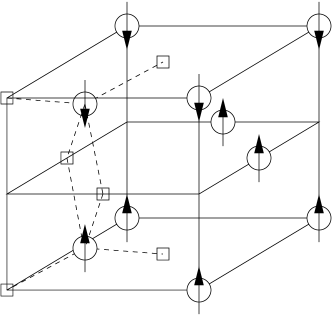
Figure 11: The most stable of the three distinct stacked-DDW structures for a tetravacancy cluster in fct afmD Fe. The arrows indicate the local moments on the Fe atoms (circles) and the magnetic planes are shown explicitly. Vacancies are shown as small squares. The two central Fe atoms repel one another away from their relaxed positions in the DDW sub-units but maintain the large moments of around $3\ \mu_{\mathrm{B}}$ found previouslyKlaver12 .

Following work in fcc AlWang2011 we considered the natural growth of these highly-stable DDW-type structures by investigating tetravacancy clusters of the form shown in Fig. 11, which we refer to as stacked-DDW structures. In pure Fe we found them to be more stable than all other tetravacancy clusters considered previouslyKlaver12 , with a total binding energy in the range $1.00\pm 0.29$ eV. The corresponding vac₄-Y clusters were then investigated by replacing a central Fe atom with a Y solute. In contrast to the pure Fe case, where the binding energy is around 0.4 eV higher than for the trivacancy, the total binding energies for these vac₄-Y clusters, at around 4.9 eV, are lower than the most stable vac₃-Y cluster. We also considered forming vac₄-Y clusters by placing a Y solute within the most open vac₅ clusters, which are square-based pyramidal in formKlaver12 . While the total binding energy did increase to 5.06 eV, $E_{\mathrm{b}}^{\mathrm{vac}}$ is still negative [see Table 4]. We conclude that the concentration of vac₄-Y clusters will be relatively low in thermal equilibrium. Finally, we considered the vac₅-Y cluster with a Y atom at the centre of an octahedral hexavacancyKlaver12 , as this structure was found to be highly-stable in fcc CuVineyard1961 , fcc AlWang2011 and fct afmD FeKlaver12 . The total binding energy increases significantly, which confirms the cluster’s stability. Their growth, however, will be inhibited by the instability of the vac₄-Y cluster. Divacancy absorption by a vac₃-Y cluster represents an alternative, and plausible, formation mechanism, although in this case limited by the divacancy concentration.

Overall, the presence of Y (and other oversized solutes) in the Fe matrix provide a high capacity for the trapping of vacancies, primarily through the formation of highly-stable clusters, such as vac₃-Y and vac₅-Y. Not only will this reduce the effective mobility of vacancies but these clusters should act as natural recombination sites, reducing the net concentrations of both vacancy and self-interstitial point defects in the metal. While the oversized solutes do act as nucleation sites for voids, their net effect will be to inhibit the growth of large voids and interstitial loops and reduce the swelling of the material under irradiation. These observations also suggest the possibility that if any oversized solutes used in the production of ODS steels, such as Y, Hf and Ti, remain dissolved in the Fe matrix they would contribute to the observed radiation-damage resistance of these materials and complement the action of the complex oxide nanoparticles as point defect sinks and recombination sitesBrodrick2014 ; Oka2011 .

III.3 TM Solute interactions with self-interstitial defects

In austenite, as in all other fcc metals, the $\langle 001\rangle$ dumbbell is the most stable self-interstitial defectKlaver12 and is highly mobile with a migration energy in the range from 0.20 to 0.25 eVHepburn13 . The dumbbell produces an anisotropic distortion of the local lattice, putting the neighbouring atoms under either compression or tension, which generally leads to repulsion or attraction to oversized solutes placed in these sites, respectivelyOlsson10 . In this work we have studied the interactions of TM solutes with the [001] self-interstitial dumbbell (SI), paying particular attention to those configurations exhibiting positive binding, where the solutes can act as traps for self-interstitial defects. We start, however, by considering the solute binding energies in the mixed dumbbell, $E_{\mathrm{b}}(\mathrm{SI,X;mix})$, which is the most compressive solute environment. The results are shown in Fig. 12.

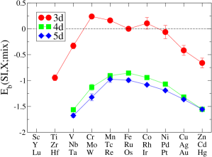
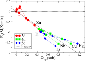
Figure 12: SI-solute binding energies for the mixed dumbbell configuration, $E_{\mathrm{b}}(\mathrm{SI,X;mix})$, in eV (a) across the TM series and (b) versus the solute size factor, $\Omega_{\mathrm{SF}}(\mathrm{sub})$, in fct afmD Fe. The error bars identify the spread in binding energies over the two distinct mixed dumbbell configurations in the fct afmD structure, with the data point chosen at the centre of this range. Note that for Ag, Cd and Hg only one of the mixed dumbbells was found to be stable. Figure (b) also shows the result of a linear fit to the combined dataset, $E_{\mathrm{b}}=-1.73\ \Omega_{\mathrm{SF}}$. The data is given in Appendix B.

The interactions are, generally, repulsive with a strength that increases with the solute size factor. In fact, the binding energy data can be successfully modelled as a linear function of the size factor with a proportionality constant of -1.73 eV, which compares with a value of -2.03 eV in bcc FeOlsson10 . The solute atom in a mixed dumbbell was also observed to move progressively closer to the dumbbell lattice site, at the expense of its Fe partner, as the size factor increased. For the largest solutes, namely Sc, Y, Lu, Zr, Hf, Ag, Cd and Hg, this tendency resulted in (at least one of) the mixed dumbbells becoming unstable, with the solute, effectively, occupying the lattice site and pushing its Fe partner away to form an SI in either the 2b or 2c configuration [see Fig. 5]. In contrast to these general results, the magnetic elements Cr, Mn, Co and (to some extent) Ni bind positively to the mixed dumbbell. The attractive interactions for Cr and Mn, in particular, stand clearly apart from the general trend with size factor [see Fig. 12]. There is, however, some consistency in their interactions with point defects, as they are repelled from the vacancy [see Fig. 4], exhibiting behaviour that would be intuitively expected of undersized solutes, despite their observed sizesKlaver12 .

As well as the mixed dumbbell, configurations where the solute occupies a compressive site at 1nn to the SI [sites 1b and 1c in Fig. 5] are critically important in interstitial-mediated solute diffusionTucker10 . For the 3d solutes, the trend in binding energy data [see Appendix B] follows a very similar pattern to that for the mixed dumbbell. Once again, Cr, Mn, Co and (to some extent) Ni exhibit positive binding while the oversized solutes are repelled, although to a much lesser extent than from the mixed dumbbell. It is interesting to note that V is positively bound to the SI in the 1nn compressive sites, despite being repelled from the mixed dumbbell. We conclude that interstitial-mediated diffusion is only likely to be important for the magnetic solutes, with the effect being most pronounced for Cr and Mn.

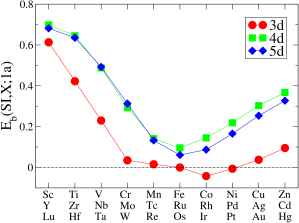
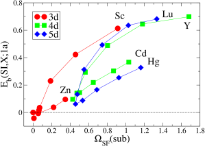
Figure 13: SI-solute binding energies for the 1nn tensile configuration, $E_{\mathrm{b}}(\textrm{SI,X;1a})$, in eV (a) across the TM series and (b) versus the solute size factor, $\Omega_{\mathrm{SF}}(\mathrm{sub})$, in fct afmD Fe. This configuration is uniquely defined in the fct afmD structure, with the solute at site 1a in Fig. 5. The data is given in Appendix B.

In contrast to the two cases above, we observed, almost exclusively, attractive interactions for solutes in the 1nn tensile site near an SI [site 1a in Fig. 5]. The binding energies, $E_{\mathrm{b}}(\textrm{SI,X;1a})$, in Fig. 13 exhibit clear trends across the TM series and the data clearly differentiates between the 3d and 4d/5d solutes. The strength of binding does increase with the solute size factor but the early and late TMs follow quite distinct trends [Fig. 13], as observed for other quantities here and in bcc FeOlsson10 . The binding energies for the late TM solutes are, approximately, proportional to their size factors with a proportionality coefficient of around 0.3 eV and while the binding energies for the early TM solutes do increase at a greater (non-linear) rate, the data appears to saturate for $\Omega_{\mathrm{SF}}>1$.

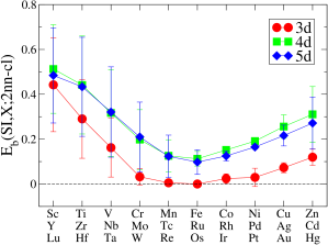
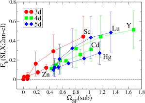
Figure 14: SI-solute binding energies, $E_{\mathrm{b}}(\textrm{SI,X;2nn-cl})$, in eV for solutes at 2nn and in sites collinear with the [001] self-interstitial defect (a) across the TM series and (b) versus the solute size factor, $\Omega_{\mathrm{SF}}(\mathrm{sub})$, in fct afmD Fe. The error bars identify the spread in binding energies over the two distinct sites, namely 2b and 2c in Fig. 5, with the data point chosen at the centre of this range. The data is given in Appendix B.

Positive binding energies of up to the same magnitude and following very similar (average) trends [see Fig. 14] were also observed for solutes in the 2nn sites collinear with the [001] dumbbell [sites 2b and 2c in Fig. 5]. While the large spread in the data does preclude a detailed analysis, the binding energy clearly increases with solute size factor. Calculations for the 3d solutes in the 2a site [see Fig. 5] found only weak binding [see Appendix B], that was positively correlated to the solute size factor.

Overall, we have demonstrated that oversized TM solutes can act as strong trapping sites for SI defects and that this effect increases with the solute size factor. Their addition to austenitic steels should, therefore, not only act to reduce the effective mobility of SI defects but lead to enhanced recombination rates and a reduction in the net defect concentrations under irradiation. The data also suggests that oversized TM solutes will act as nucleation sites for self-interstitial clusters.

IV Conclusions

In this work we have extended the theoretical database of atomic-level properties of steels by performing a comprehensive set of first principles electronic structure calculations to study transition metal solute properties in austenite and their interactions with point defects.

We have found clear trends in the properties of substitutional TM solutes in the defect-free lattice, their binding energies to point defects and in quantities relevant to vacancy-mediated solute diffusion across the TM series, as a function of the local d band occupancy of the solute atoms. The interaction data between TM solutes and point defects are highly correlated to the solute size factors in a way that is consistent with arguments based on elasticity and local strain field effects. Functional dependencies can generally be used to model these relationships, although in some cases the early and late TM solutes show quite distinct behaviour, as observed in bcc FeOlsson10 . Throughout this work we have observed high levels of consistency and strong correlation between results in fct afmD Fe and bcc fm FeOlsson10 , which adds to similar observations made previouslyKlaver12 ; Hepburn13 . We would expect this insensitivity to the crystal structure to extend to other solvent metals.

We have shown that oversized TM solutes act as strong traps for both vacancy and self-interstitial defects, with a strength that increases with the solute size factor. Furthermore, we have shown, using Y as a representative, that oversized solutes act as strong traps for additional vacancies, forming close-packed vacancy clusters around a central solute. The vac₃-X and vac₅-X clusters were found to form particularly stable configurations. Our previous analysisKlaver12 suggests that highly-stable clusters of aligned self-interstitial dumbbells should form around a single solute atom. This high trapping capacity should result in a significant lowering of defect mobility and reduction in the net concentration of point defects in the matrix, both by enhancing defect recombination and by providing nucleation sites for the formation of secondary defects, such as proto-voidsKato1991 and interstitial loops. Overall, these observations provide a strong foundation for the suggestion by Kato et al.Kato1991 ; Kato1992 , that point defect trapping at oversized TM solutes underlies their experimental observations of reduced swellingKato1991 and a decrease in RISKato1992 in 316L austenitic steel doped with small concentrations of solutes. The same conclusions also apply to ODS steels where any oversized solutes, such as Y, Hf and Ti, remaining dissolved in the Fe matrix after manufacture would contribute to the radiation-damage resistance provided by the oxide nanoparticlesBrodrick2014 ; Oka2011 .

We have extended our previous analysisKlaver12 of vacancy-mediated solute diffusion to cover Cr, Mn, Co, Ni and Cu. We find that Ni and Co diffuse at similar rates below that of Fe and will diffuse with the vacancy flux by the vacancy drag mechanism below a critical temperature, which for Co is $400\pm 50$ K. In contrast, both Cr and Cu diffuse more quickly than Fe and Mn at an intermediate rate against the vacancy flux. We infer that the concentrations of Co and Ni will be enhanced and those of Cr and Cu depleted at defect sinks.

We have demonstrated a reduction in the migration barrier for vacancy-solute exchange at 1nn ($\omega_{2}$ jumps) as the solute size factor increases. For sufficiently large solutes, namely Sc, Y, Zr, Lu and Hf, the barrier ceases to exist and the solute, X, stably binds to the vacancy at a position half way between the two lattice sites to form an SCD defect. This is the transition state configuration for the smaller solutes. For those solutes forming a stable SCD, or for those where the $\omega_{2}$ jump barrier is below the thermal energy $k_{\mathrm{B}}T$, namely Ti, Nb and Ta, vacancy-mediated solute diffusion is dominated by the $\omega_{3}$ dissociation/reassociation mechanism identified in this work. The activation energy for this process is lower than that for self-diffusion, which is in contrast to the, often assumed, immobility of such large solutes. This important result should be taken account of in future studies of the nucleation and growth of complex oxide nanoparticles in ODS steels.

Interstitial-mediated solute diffusion will be energetically disfavoured in proportion to the solute size factor for all solutes except Cr, Mn, Co and (to a lesser extent) Ni, where, magnetic effects lead to favourable interactions with the self-interstitial defect. Even for these solutes, the relative contribution compared to vacancy-mediated diffusion will depend critically on the concentrations of the respective defects in the matrix and a definitive study is well beyond the scope of this workTucker10 .

Finally, we note that since the majority of our conclusions are based on solute size factor effects they should generalise to other solvent metals and to concentrated austenitic steels in particular.

V Acknowledgements

This work was part sponsored through the EU-FP7 PERFORM-60 project, the G8 funded NuFUSE project and EPSRC through the UKCP collaboration.

Appendix A Elemental data and ground state crystal structure calculations

We performed a set of high-precision ab initio calculations for the ground state (0K) crystalline and magnetic structures of all the transition metals (TMs), primarily for use as reference states in the determination of formation energies for the TM solute calculations presented in this work. Aside from Mn and Fe, these crystal structures are either hexagonal close-packed (hcp), body-centred cubic (bcc), face-centred cubic (fcc) or rhombohedral (rho) and the magnetic structures either non-magnetic (nm), ferromagnetic (fm) or antiferromagnetic (afm). The ground state crystallographic parameters were determined by full relaxation of the unit cell and atomic positions. To ensure that the unit cell stress tensor and, therefore, lattice parameters were determined accurately we used a plane-wave energy cutoff of 550 eV, a high-density Monkhorst-Pack k-point grid to sample the Brillouin zone [see Table 5] and an energy tolerance of $10^{-8}$ eV to converged the electronic ground state. For the structural relaxations, forces were converged to less than $10^{-4}$ eV/$\mathrm{\AA}$ and the cell stress to less than $5\times 10^{-6}$ eV/$\mathrm{\AA}^{3}$ (0.008 kB). Detailed calculations showed that these settings were sufficient to converge the energy to better than 0.5 meV/atom, the pressure to $5\times 10^{-4}$ eV/$\mathrm{\AA}^{3}$ (0.8 kB) and local magnetic moments to $10^{-3}\ \mu_{\mathrm{B}}$, resulting in errors to the lattice parameters of much less than 0.001 $\mathrm{\AA}$. The results are given in Table 5 for all elements except Mn, which we now discuss in more detail.

Element	$N_{\mathrm{val}}$ : Config.	$r_{\mathrm{wigs}}$	k-points	Crystal structure and parameters	$E_{\mathrm{coh}}$
Sc	11 : 3s23p63d14s2	1.429	16x16x12	hcp, nm, $a=3.314\ \mathrm{\AA}$, $c=5.144\ \mathrm{\AA}$	3.90
Ti	10 : 3p63d24s2	1.323	16x16x12	hcp, nm, $a=2.932\ \mathrm{\AA}$, $c=4.642\ \mathrm{\AA}$	4.85
V	11 : 3p63d34s2	1.217	20x20x20	bcc, nm, $a=2.996\ \mathrm{\AA}$	5.31
Cr	6 : 3d54s1	1.323	20x20x20	bcc, afm, $a=2.849\ \mathrm{\AA}$, $|\mu|=0.92\ \mu_{\mathrm{B}}$	4.10
Mn	7 : 3d54s2	1.323	6x6x6	$\alpha$-Mn [see Table 6]	2.92
Fe	8 : 3d64s2	1.302	20x20x20	bcc, fm, $a=2.832\ \mathrm{\AA}$, $\mu=2.20\ \mu_{\mathrm{B}}$	4.28
			16x16x8	fct, afmD, $a=3.447\ \mathrm{\AA}$, $c=3.750\ \mathrm{\AA}$, $|\mu|=1.99\ \mu_{\mathrm{B}}$	4.20
			16x16x16	fcc, nm, $a=3.447\ \mathrm{\AA}$	4.06
Co	9 : 3d74s2	1.302	18x18x10	hcp, fm, $a=2.495\ \mathrm{\AA}$, $c=4.028\ \mathrm{\AA}$, $\mu=1.62\ \mu_{\mathrm{B}}$	4.39
Ni	10 : 3d84s2	1.286	18x18x18	fcc, fm, $a=3.522\ \mathrm{\AA}$, $\mu=0.63\ \mu_{\mathrm{B}}$	4.44
Cu	11 : 3d104s1	1.312	18x18x18	fcc, nm, $a=3.636\ \mathrm{\AA}$	3.49
Zn	12 : 3d104s2	1.270	20x20x16	hcp, nm $a=2.643\ \mathrm{\AA}$, $c=5.080\ \mathrm{\AA}$	1.35
Y	11 : 4s24p64d15s2	1.815	16x16x12	hcp, nm, $a=3.649\ \mathrm{\AA}$, $c=5.661\ \mathrm{\AA}$	4.37
Zr	12 : 4s24p64d25s2	1.625	16x16x12	hcp, nm, $a=3.232\ \mathrm{\AA}$, $c=5.180\ \mathrm{\AA}$	6.25
Nb	11 : 4p64d45s1	1.503	20x20x20	bcc, nm, $a=3.323\ \mathrm{\AA}$	7.57
Mo	12 : 4p64d55s1	1.455	20x20x20	bcc, nm, $a=3.172\ \mathrm{\AA}$	6.82
Tc	13 : 4p64d65s1	1.423	20x20x16	hcp, nm, $a=2.764\ \mathrm{\AA}$, $c=4.420\ \mathrm{\AA}$	6.85
Ru	8 : 4d75s1	1.402	20x20x16	hcp, nm, $a=2.729\ \mathrm{\AA}$, $c=4.304\ \mathrm{\AA}$	6.74
Rh	9 : 4d85s1	1.402	18x18x18	fcc, nm, $a=3.844\ \mathrm{\AA}$	5.75
Pd	10 : 4d105s0	1.434	18x18x18	fcc, nm, $a=3.956\ \mathrm{\AA}$	3.89
Ag	11 : 4d105s1	1.503	18x18x18	fcc, nm, $a=4.157\ \mathrm{\AA}$	2.95
Cd	12 : 4d105s2	1.577	20x20x16	hcp, nm, $a=3.023\ \mathrm{\AA}$, $c=5.798\ \mathrm{\AA}$	1.16
Lu	9 : 5p65d16s2	1.588	16x16x12	hcp, nm, $a=3.514\ \mathrm{\AA}$, $c=5.460\ \mathrm{\AA}$	4.43
Hf	10 : 5p65d26s2	1.614	20x20x16	hcp, nm, $a=3.199\ \mathrm{\AA}$, $c=5.054\ \mathrm{\AA}$	6.44
Ta	11 : 5p65d36s2	1.503	20x20x20	bcc, nm, $a=3.320\ \mathrm{\AA}$	8.10
W	12 : 5p65d46s2	1.455	20x20x20	bcc, nm, $a=3.190\ \mathrm{\AA}$	8.90
Re	7 : 5d56s2	1.455	18x18x14	hcp, nm, $a=2.779\ \mathrm{\AA}$, $c=4.485\ \mathrm{\AA}$	8.03
Os	14 : 5p65d66s2	1.413	20x20x16	hcp, nm, $a=2.761\ \mathrm{\AA}$, $c=4.357\ \mathrm{\AA}$	8.17
Ir	9 : 5d96s0	1.423	18x18x18	fcc, nm, $a=3.882\ \mathrm{\AA}$	6.94
Pt	10 : 5d96s1	1.455	18x18x18	fcc, nm, $a=3.985\ \mathrm{\AA}$	5.84
Au	11 : 5d106s1	1.503	18x18x18	fcc, nm, $a=4.173\ \mathrm{\AA}$	3.81
Hg	12 : 5d106s2	1.614	26x26x26	rho, nm, $a=3.101\ \mathrm{\AA}$, $\gamma=84.4^{\circ}$	0.67

Table 5: Calculation details and ground state properties for the transition metals elements considered in this work. In particular we give the number of valence electrons in the PAW potential, $N_{\mathrm{val}}$, and the atomic valence electron configurationKittel , the atomic radius used for calculating local magnetic moments, $r_{\mathrm{wigs}}$, in $\mathrm{\AA}$, the dimensions of the k-point grid used to sample the Brillouin zone, the equilibrium crystal and magnetic structure parameters for the conventional unit cell (at T=0K) and the experimental cohesive energy per atom at T=0K [from KittelKittel , p.50], $E_{\mathrm{coh}}$, in eV. The values of $E_{\mathrm{coh}}$ for the fct afmD and fcc nm states of Fe were estimated using the ab initio energy differences to the bcc fm ground state of 0.077 and 0.216 eV/atom, respectivelyKlaver12 , and experimental ground state cohesive energy.

The crystalline structure of Mn differs distinctly from the other transition metals. Under standard conditions of temperature and pressure the most stable polymorph, $\alpha$-Mn, is paramagnetic (para) with a 58 atom body-centred cubic unit cell with space group $\mathrm{T}^{3}_{\mathrm{d}}-\mathrm{I}\bar{4}3\mathrm{m}$ (number 217), as first resolved by Bradley and ThewlisBradley1927 . They found a lattice parameter, $a=8.894\ \mathrm{\AA}$, and four crystallographically distinct sets of atomic positions. Using the nomenclature of Hobbs et al.Hobbs01 ; Hobbs03 their number, Wyckoff positions and internal coordinates relative to $[(0,0,0),(\frac{1}{2},\frac{1}{2},\frac{1}{2})]$ are as follows: 2 type-I atoms at (a), $[(0,0,0)]$; 8 type-II atoms at (c), $[(x,x,x),(x,-x,-x),(-x,x,-x),(-x,-x,x)]$ and two sets of 24 atoms, type-III and type-IV, at (g), $[(x,x,z),(x,-x,-z),(-x,x,-z),(-x,-x,z)]+$ cyclic permutations. A more recent and accurate study by Yamada et al. used single crystal measurements to extrapolate the crystallographic parameters of para $\alpha$-Mn to 0 KYamada1970 . The results are summarised in Table 6.

Authors	Bradley &	Yamada	Lawson	Hobbs	Hobbs	This	This
	ThewlisBradley1927	et al.Yamada1970	et al.Lawson1994	et al.Hobbs03	et al.Hobbs03	work	work
Magnetism	para	para	afm	nm	afm	nm	afm
$a$	8.894	8.865	8.877	8.532	8.669	8.546	8.636
$c$			8.873		8.668
$V_{\mathrm{atom}}$	12.13	12.01	12.06	10.71	11.23	10.76	11.10
$x(\mathrm{II})$	$0.31_{7}$	0.317	0.3192(2)	0.318	0.320	0.318	0.319
$z(\mathrm{II})$			0.3173(3)		0.319
$x(\mathrm{IIIa})$	$0.35_{6}$	0.357	0.3621(1)	0.356	0.355	0.356	0.356
$x(\mathrm{IIIb})$			0.3533(2)		0.355
$z(\mathrm{IIIb})$			0.3559(2)		0.354
$z(\mathrm{IIIa})$	$0.04_{2}$	0.034	0.0408(2)	0.037	0.032	0.037	0.035
$y(\mathrm{IIIb})$			0.0333(1)		0.033
$x(\mathrm{IVa})$	$0.08_{9}$	0.089	0.0921(2)	0.088	0.088	0.088	0.088
$x(\mathrm{IVb})$			0.0895(2)		0.088
$z(\mathrm{IVb})$			0.0894(2)		0.087
$z(\mathrm{IVa})$	$0.27_{8}$	0.282	0.2790(3)	0.281	0.283	0.281	0.283
$y(\mathrm{IVb})$			0.2850(1)		0.283
$\mu(\mathrm{I})$	—	—	2.83(13)	—	2.79	—	2.86
$\mu(\mathrm{II})$	—	—	1.83(06)	—	2.22	—	2.31
$\mu(\mathrm{IIIa})$	—	—	0.74(14)	—	-1.11	—	-1.23
$\mu(\mathrm{IIIb})$	—	—	-0.48(11)	—	-1.10	—	-1.23
$\mu(\mathrm{IVa})$	—	—	-0.59(10)	—	0.0	—	$|\mu|$
$\mu(\mathrm{IVb})$	—	—	0.66(07)	—	0.0	—	$<0.03$

Table 6: Crystallographic parameters for $\alpha$-Mn. The lattice parameters, $a$ and $c$, are in $\mathrm{\AA}$, the atomic volume, $V_{\mathrm{atom}}$, in $\mathrm{\AA}^{3}$ and the other internal parameters are dimensionless. The results of Yamada et al.Yamada1970 are for para $\alpha$-Mn extrapolated to 0 K. The results of Lawson et al.Lawson1994 were measured at 15 K. Magnetic moments, $\mu$, are given in $\mu_{\mathrm{B}}$ for the distinct atomic types centred on (0,0,0), with the moments around $(\frac{1}{2},\frac{1}{2},\frac{1}{2})$ anti-parallel to these. For the non-collinear structure of Lawson et al.Lawson1994 the magnitudes of the moments are given and the sign indicates the moment direction when projected onto the MnI moments about (0,0,0). It should be noted that the relative orientations of the moments from Hobbs et al.Hobbs03 were determined from figures in that work given the lack of clarity in their specification in the text and tables.

Low-temperature neutron diffraction studies by Shull and WilkinsonShull1953 found that $\alpha$-Mn is afm below a Néel temperature of 95 K. Further studies to resolve the magnetic structureKasper1956 ; Oberteuffer1968 ; Kunitomi1969 ; Yamada1970 ; Lawson1994 were complicated by the need to use theoretical models to analyse and interpret the diffraction data, resulting in a number of both collinear and non-collinear magnetic structures exhibiting a whole range of magnetic moments. Kunitomi et al.Kunitomi1969 showed that a non-collinear model was necessary to reproduce the experimental results and the magnetic structure then resolved by Yamada et al.Yamada1970 following a group-theoretical approachYamada1970b , although with some remaining variability in the moments depending on the exact details of the model used. More recent work by Lawson et al.Lawson1994 used a Shubnikov (magnetic space) group-based analysis, yielding an anti-body-centred tetragonal magnetic structure, equivalent to Yamada et al.Yamada1970 . Furthermore, they were able to determine that the implied body-centred and weakly tetragonal crystal structure belongs to space group $\mathrm{I}\bar{4}2\mathrm{m}$ (number 121), with the four distinct sets of atoms in the paramagnetic case now split into six: The 2 type-I atoms are unchanged, the 8 type-II atoms now take Wyckoff position (i), $[(x,x,z),(x,-x,-z),(-x,x,-z),(-x,-x,z)]$ and the 24 type-III and type-IV atoms now split into two distinct subsets with 8 atoms (IIIa/IVa) at position (i) and 16 (IIIb/IVb) at (j), $[(x,y,z)$, $(x,-y,-z)$, $(-x,y,-z)$, $(-x,-y,z)$, $(y,x,z)$, $(y,-x,-z)$, $(-y,x,-z)$, $(-y,-x,z)]$. Determinations of the crystallographic parameters at a number of temperatures from 305 to 15 KLawson1994 clearly shows the onset of the magnetic transition with its coupled tetragonal distortion of the lattice and the splitting of the internal coordinates below the Néel temperature so that $x(\mathrm{II})\neq z(\mathrm{II})$, $x(\mathrm{IIIa}),x(\mathrm{IIIb}),z(\mathrm{IIIb})\neq x(\mathrm{III})$ and $z(\mathrm{IIIa}),y(\mathrm{IIIb})\neq z(\mathrm{III})$, with equivalent results for the type-IV atoms. Along with Bradley and ThewlisBradley1927 they also make the interesting point that the complexity of the $\alpha$-Mn structure (as compared to the other TMs) can be understood once viewed as a self-intermetallic compound between Mn atoms in crystallographically distinct sites with distinct electronic/magnetic configurations and, therefore, different atomic sizes. The results of Lawson et al.Lawson1994 are summarised in Table 6.

Theoretical attempts to model $\alpha$-Mn culminate in a comprehensive ab initio study by Hobbs et al.Hobbs01 ; Hobbs03 , who also provide an excellent summary and discussion of the preceding theoretical and experimental work on Mn. The other polymorphs of Mn are considered in related workHobbs01 ; Hobbs03II ; Hafner05 . Their study covers the nm state and both collinear and non-collinear afm magnetic states of $\alpha$-Mn over a range of atomic volumes. For the nm state they find a low equilibrium atomic volume of 10.71 $\mathrm{\AA}^{3}$ ($a=8.532\ \mathrm{\AA}$). The equilibrium afm state lies around 0.025 eV/atom lower than the nm state (as determined from their energy vs volume curves) at an atomic volume of 11.23 $\mathrm{\AA}^{3}$ and exhibits a collinear magnetic structure with only marginal evidence of any tetragonal distortion [see Table 6]. It is only above the experimental volume ( 12 $\mathrm{\AA}^{3}$/atom) that any appreciable non-collinearity in the magnetic structure and tetragonal lattice distortion is observed, which they suggest is closely related to the critical development of non-zero moments on MnIV atoms.

The results of our own calculations are summarised in Table 6. We find that the nm state of $\alpha$-Mn has an equilibrium volume of 10.76 $\mathrm{\AA}^{3}$ ($a=8.546\ \mathrm{\AA}$), in good agreement with Hobbs et al.Hobbs01 ; Hobbs03 . Our use of a finer $6^{3}$ k-point grid may explain the slight discrepancy. It is often said that Mn would resort to an hcp structure, like the other group VII TMs Tc and Re, in the absence of magnetism. We, however, find the surprising result that the equilibrium nm hcp structure ($a=2.478\ \mathrm{\AA}$, $c=4.004\ \mathrm{\AA}$) lies 45 meV/atom above nm $\alpha$-Mn. This also indicates that the primary mechanism driving the formation of the complex $\alpha$-Mn structure is not magnetic in origin.

Determination of the afm structure was significantly more complex. For the magnetic structure we initialised the moments on MnIV atoms to zero, following Hobbs et al.Hobbs03 . For consistency with the experimental and theoretical results in the literature we take the moments on atoms of the same type to be equal in magnitude but with anti-parallel orientations about (0,0,0) and $(\frac{1}{2},\frac{1}{2},\frac{1}{2})$ (to produce the afm structure). With these assumptions there are still 16 distinct relative orientations of moments between the different atomic types for the tetragonal structure. Calculations were initialised in all of these distinct magnetic states with either cubicGazzara1966 or tetragonalLawson1994 ; Hobbs03 lattice parameters. Despite many distinct magnetic states being initially stable only one stable afm structure was found after full relaxation [see Table 6].

We found a cubic afm structure with an atomic volume of 11.10 $\mathrm{\AA}^{3}$ ($a=8.636\ \mathrm{\AA}$), which is 8.0% (2.7%) lower than experimentLawson1994 , although this is typical of GGA calculations on afm systemsHobbs03 . We found no evidence of a stable tetragonally distorted lattice, unlike Hobbs et al.Hobbs01 ; Hobbs03 although their calculations only show a very marginal effect. The energy difference between the nm and afm states of $\alpha$-Mn, that we measure to be 28 meV/atom, does, interestingly, agree well with Hobbs et al.. The internal coordinates show a high degree of consistency both with the nm state from this work and with other theoreticalHobbs01 ; Hobbs03 and experimentalBradley1927 ; Yamada1970 ; Lawson1994 ; Gazzara1966 work, although this is, perhaps, not surprising given their relative invariance as a function of temperature above and below the magnetic transitionLawson1994 . For the magnetic structure we find large moments on MnI and MnII atoms, that agree qualitatively with the (near)-collinear moments found in other workHobbs03 ; Lawson1994 , and smaller moments on MnIII and MnIV atoms, consistent with the majority of previous studies [see Hobbs et al.Hobbs03 and references therein]. While the MnIII moments are similar in magnitude to those from experimentLawson1994 we found that our calculations did not differentiate between MnIIIa and MnIIIb atoms, despite initialising their positions consistent with a tetragonal structureHobbs03 ; Lawson1994 and their moments to be either parallel or anti-parallel and with different magnitudes. Along with Hobbs et al.Hobbs03 we also found near-zero equilibrium moments on MnIV atoms, in contrast with experimentLawson1994 . Given that Hobbs et al.Hobbs01 ; Hobbs03 report the generation of non-collinearity in MnIII and MnIV moments as well as non-zero MnIV moments at volumes exceeding equilibrium, it is certainly plausible that the failure of theory to produce the correct magnetic state at equilibrium is closely related to its underestimation of the atomic volume. Overall, we conclude that the afm state we have found is the best-possible reproduction of the ground-state structure for $\alpha$-Mn within the particular theoretical framework used in this work.

Appendix B TM solute data

In this appendix, we present the data from the large supercell calculations used in this work. The data is given at the precision of the VASP output for reproducibility and further use and should not be taken to indicate the accuracy of the results. Substitutional TM solute properties in fct afmD and bcc fm Fe are given in Table 7. Vacancy-solute binding energies at 1nn separation and vacancy migration energies for the five-frequency model jumps in fct afmD Fe are given in Table 8. Binding energies between TM solutes and an [001] self-interstitial dumbbell at up to 2nn separation in fct afmD Fe are given in Table 9. Vacancy-Y binding energies at 2nn, 3nn and 4nn separations in fct afmD Fe are given in Table 10. Migration energies for $\omega_{3}$ vacancy jumps near a Y solute in fct afmD Fe are given in Table 11.

	fct afmD Fe			bcc fm Fe
	$E_{\mathrm{f}}(\mathrm{sub})$	$\mu(\mathrm{sub})$	$\Omega_{\mathrm{SF}}(\mathrm{sub})$	$E_{\mathrm{f}}(\mathrm{sub})$	$\mu(\mathrm{sub})$	$\Omega_{\mathrm{SF}}(\mathrm{sub})$
Sc	0.423638	-0.099	0.913	0.315274	-0.394	0.665
Ti	-0.376736	-0.144	0.457	-0.805544	-0.757	0.381
V	-0.144885	-0.070	0.188	—	—	—
Cr	0.271619	0.847	0.070	—	—	—
Mn	0.064990	1.999	0.063	—	—	—
Co	0.179164	0.978	0.009	—	—	—
Ni	0.087110	0.039	0.056	—	—	—
Cu	0.511519	-0.007	0.221	0.752995	0.111	0.218
Zn	0.207554	-0.013	0.347	0.326639	-0.081	0.342
Y	1.994622	-0.084	1.680	2.094273	-0.279	1.310
Zr	0.600812	-0.098	1.180	0.377658	-0.467	1.015
Nb	0.378045	-0.076	0.803	—	—	—
Mo	0.472454	0.068	0.563	—	—	—
Tc	0.258085	0.238	0.472	—	—	—
Ru	0.265435	0.295	0.427	—	—	—
Rh	0.081337	0.158	0.502	—	—	—
Pd	0.490826	0.017	0.649	—	—	—
Ag	1.756191	-0.009	0.867	1.914812	0.100	0.937
Cd	1.746557	-0.012	1.032	1.883467	-0.064	0.951
Lu	1.197321	-0.109	1.334	1.233167	-0.372	1.035
Hf	0.235090	-0.099	1.027	-0.016113	-0.468	0.891
Ta	0.128539	-0.068	0.745	—	—	—
W	0.457315	0.005	0.550	—	—	—
Re	0.243007	0.136	0.476	—	—	—
Os	0.233483	0.217	0.457	—	—	—
Ir	-0.169113	0.170	0.533	—	—	—
Pt	-0.105044	0.044	0.687	—	—	—
Au	1.072340	-0.006	0.924	1.069742	0.171	1.073
Hg	2.053529	-0.012	1.161	2.157507	-0.031	1.197

Table 7: The formation energy, $E_{\mathrm{f}}(\mathrm{sub})$, in eV, magnetic moment (in an up-spin magnetic plane for fct afmD Fe), $\mu(\mathrm{sub})$, in $\mu_{\mathrm{B}}$ and size factor, $\Omega_{\mathrm{SF}}(\mathrm{sub})$, for substitutional transition metal solutes in fct afmD and bcc fm Fe.

	$E_{\mathrm{b}}(\mathrm{vac,X;1a})$	$E_{\mathrm{b}}(\mathrm{vac,X;1b})$	$E_{\mathrm{b}}(\mathrm{vac,X;1c})$	$E_{\mathrm{m}}(\omega_{2};\mathrm{1a})$	$E_{\mathrm{m}}(\omega_{2};\mathrm{1b})$	$E_{\mathrm{m}}(\omega_{1};\mathrm{1b}\rightarrow\mathrm{1b})$	$E_{\mathrm{m}}(\omega_{1};\mathrm{1c}\rightarrow\mathrm{1c})$
Sc	0.750650	0.499434	0.505687	0.000000	0.004553	1.597425	1.203072
Ti	0.277210	0.106405	0.137513	0.036143	0.118099	1.150778	0.868661
V	0.095458	-0.024377	0.002539	0.264122	0.421619	0.897122	0.717379
Cr	0.003838	-0.074678	-0.090630	0.559822	0.741722	0.731824	0.672854
Mn	0.004220	-0.062333	-0.069264	0.674926	1.097378	0.746450	0.740400
Co	0.023113	0.038358	0.010414	0.903159	1.142975	0.728135	0.685638
Ni	0.056450	0.027066	0.016082	0.891343	1.172443	0.779333	0.638315
Cu	0.121276	0.033691	0.071821	0.679113	0.939329	0.839959	1.084078
Zn	0.194651	0.063915	0.139639	0.469792	0.664598	0.909838	0.714105
Y	1.391114	1.146585	1.298059	0.000000	0.000000	2.225764	1.900111
Zr	0.885999	0.611256	0.624385	0.000000	0.000000	1.713237	1.354309
Nb	0.410330	0.178429	0.266261	0.039749	—	—	—
Mo	0.224573	0.031336	0.071605	0.351614	—	—	—
Tc	0.144515	0.013633	-0.024236	0.700993	—	—	—
Ru	0.137180	0.050221	-0.021785	0.953080	—	—	—
Rh	0.192630	0.096389	0.041094	1.007728	—	—	—
Pd	0.276956	0.142563	0.140851	0.808536	—	—	—
Ag	0.397634	0.207526	0.292348	0.500009	—	—	—
Cd	0.514102	0.277870	0.413913	0.283986	—	—	—
Lu	1.095221	0.816821	0.921025	0.000000	0.000000	1.929124	1.600727
Hf	0.688915	0.368512	0.455830	0.000000	0.000000	1.490638	1.214173
Ta	0.342817	0.115488	0.198550	0.129160	—	—	—
W	0.190974	0.005138	0.036606	0.454051	—	—	—
Re	0.120066	-0.008993	-0.047380	0.811482	—	—	—
Os	0.121133	0.035760	-0.056473	1.114752	—	—	—
Ir	0.179482	0.095967	0.014834	1.216038	—	—	—
Pt	0.277898	0.154282	0.126369	1.042552	—	—	—
Au	0.418477	0.243583	0.291266	0.675957	—	—	—
Hg	0.582178	0.353577	0.475884	0.349202	—	—	—

Table 8: Transition metal solute binding energies to a vacancy point defect, $E_{\mathrm{b}}(\mathrm{vac,X})$, in eV for the 1a, 1b and 1c configurations, migration energies for vacancy-solute exchange, $E_{\mathrm{m}}(\omega_{2})$, in eV along paths 1a and 1b and migration energies for $\omega_{1}$ jumps, $E_{\mathrm{m}}(\omega_{1})$, in eV from configuration 1b to 1b and 1c to 1c [see Figs. 5 and 6] in fct afmD Fe. A vacancy formation energy of 1.819197 eV was used to calculate the binding energies. Migration energies for $\omega_{0}$ jumps along paths 1a and 1b are 0.743409 and 1.048164 eV, respectively. For a Y solute, $\omega_{1}$ migration energies from configuration 1a to 1b and from 1b to 1a are 2.648928 and 2.404399 eV, respectively.

	$E_{\mathrm{b}}(\textrm{SI,X;mix-uu})$	$E_{\mathrm{b}}(\textrm{SI,X;mix-ud})$	$E_{\mathrm{b}}(\textrm{SI,X;1a})$	$E_{\mathrm{b}}(\textrm{SI,X;1b})$	$E_{\mathrm{b}}(\textrm{SI,X;1c})$	$E_{\mathrm{b}}(\textrm{SI,X;2a})$	$E_{\mathrm{b}}(\textrm{SI,X;2b})$	$E_{\mathrm{b}}(\textrm{SI,X;2c})$
Sc	unstable	unstable	0.613195	-0.148404	-0.239088	0.082942	0.650971	0.233076
Ti	-0.890140	-1.001952	0.422515	-0.026137	-0.043963	0.029957	0.466075	0.114717
V	-0.273120	-0.385646	0.230051	0.114587	0.114224	0.001583	0.292839	0.031147
Cr	0.279108	0.196335	0.035055	0.188501	0.193289	-0.036870	0.068725	-0.004504
Mn	0.173584	0.149788	0.015833	0.032447	0.031454	-0.035519	0.012747	-0.001813
Co	0.218336	-0.006592	-0.042215	0.069918	0.035001	-0.013967	0.003033	0.045561
Ni	0.064503	-0.190004	-0.006108	0.030123	-0.077773	-0.033833	-0.011471	0.070368
Cu	-0.322243	-0.511532	0.037862	-0.049706	-0.168800	-0.022084	0.050442	0.094807
Zn	-0.565613	-0.753655	0.095363	-0.103980	-0.196545	-0.001840	0.155897	0.083301
Y	unstable	unstable	0.698495	—	—	—	0.710074	0.315204
Zr	unstable	unstable	0.645110	—	—	—	0.659849	0.222883
Nb	-1.528735	-1.599024	0.488008	—	—	—	0.510657	0.123029
Mo	-1.072197	-1.187259	0.293452	—	—	—	0.331194	0.064893
Tc	-0.858870	-0.952616	0.141055	—	—	—	0.197384	0.054389
Ru	-0.848137	-0.863409	0.096056	—	—	—	0.144930	0.080102
Rh	-0.933354	-0.950466	0.145075	—	—	—	0.153587	0.150243
Pd	-1.031908	-1.105313	0.218741	—	—	—	0.190158	0.192314
Ag	unstable	-1.318686	0.303076	—	—	—	0.308318	0.203754
Cd	unstable	-1.556954	0.367269	—	—	—	0.434429	0.186782
Lu	unstable	unstable	0.681841	—	—	—	0.696565	0.271834
Hf	unstable	unstable	0.635332	—	—	—	0.654131	0.212396
Ta	-1.636926	-1.715900	0.492322	—	—	—	0.522191	0.119564
W	-1.256014	-1.389369	0.312929	—	—	—	0.365106	0.054661
Re	-0.914785	-1.035476	0.132741	—	—	—	0.217986	0.028394
Os	-0.955385	-1.031388	0.061411	—	—	—	0.152669	0.042942
Ir	-1.098984	-1.064321	0.087307	—	—	—	0.147562	0.102479
Pt	-1.182566	-1.200569	0.165787	—	—	—	0.174715	0.155350
Au	-1.358448	-1.369936	0.253597	—	—	—	0.262270	0.169659
Hg	unstable	-1.555926	0.327290	—	—	—	0.388016	0.154981

Table 9: Transition metal solute binding energies to an [001] self-interstitial dumbbell point defect, $E_{\mathrm{b}}(\mathrm{SI,X})$, in eV for the two distinct mixed dumbbells and for the 1a, 1b 1c, 2a, 2b and 2c configurations [see Fig. 5] in fct afmD Fe. For the mixed dumbbell the solute can lie between two up spin layers (mix-uu) or an up and down spin layer (mix-ud). A dumbbell formation energy of 3.195402 eV was used to calculate the binding energies.

Site	$E_{\mathrm{b}}$	Site	$E_{\mathrm{b}}$
2a	-0.113799	3c	0.168786
2b	-0.152349	3d	0.086246
2c	-0.098449	4a	0.218183
3a	0.005167	4b	0.079361
3b	0.018938	4c	0.106539

Table 10: Vacancy-Y binding energies, $E_{\mathrm{b}}$, in eV at 2nn, 3nn and 4nn separations [see Fig. 5] in fct afmD Fe.

Jump	$E_{\mathrm{m}}$	Jump	$E_{\mathrm{m}}$
1a$\rightarrow$2a	1.808723	1c$\rightarrow$3c	1.208250
1b$\rightarrow$2a	2.134065	1c$\rightarrow$3d	1.501190
1c$\rightarrow$2c	1.836946	1a$\rightarrow$4a	1.261512
1a$\rightarrow$3b	1.659928	1c$\rightarrow$4c	1.368114
1b$\rightarrow$3b	1.441606

Table 11: Migration energies, $E_{\mathrm{m}}$, in eV for dissociative ($\omega_{3}$) vacancy jumps near a Y solute in fct afmD Fe. The jump paths are defined by the initial and final configurations [see Figs. 5 and 6]. Migration energies for the reverse (dissociative, $\omega_{4}$) jumps can be calculated from these using the vacancy-Y binding energies in Tables 8 and 10. Jumps where the migrating Fe atom would be constrained (by the collinear calculations) to have zero moment at some point on the path have not been calculated as they would result in a significant overestimation of the migration energyKlaver12 .

References

- (1) T. Kato, H. Takahashi and M. Izumiya, Mat. Trans. JIM, 32, 921-930 (1991).
- (2) T. Kato, H. Takahashi and M. Izumiya, J. Nucl. Mater. 189, 167-174 (1992).
- (3) T.R. Allen, J.I. Cole, J. Gan, G.S. Was, R. Dropek and E.A. Kenik, J. Nucl. Mater. 342, 90-100 (2005).
- (4) I.A. Stepanov, V.A. Pechenkin, Yu.V. Konobeev, J. Nucl. Mater. 329-333, 1214-1218 (2004).
- (5) H. Kishimoto, R. Kasada, O. Hashitomi and A. Kimura, J. Nucl. Mater. 386-388, 533-536 (2009).
- (6) L.L. Hsiung, M.J. Fluss and A. Kimura, Materials Letters 64, 1782-1785 (2010).
- (7) J. Brodrick, D.J. Hepburn and G.J. Ackland, J. Nucl. Mater 445, 291-297 (2014).
- (8) H. Oka, M. Watanabe, H. Kinoshita, T. Shibayama, N. Hashimoto, S. Ohnuki and S. Yamashita, J. Nucl. Mater. 417, 279-282 (2011).
- (9) H. Oka, M. Watanabe, N. Hashimoto, S. Ohnuki, S. Yamashita and S. Ohtsuka, J. Nucl. Mater. 442, 164-168 (2013).
- (10) Y. Xu, Z. Zhou, M. Li and P. He, J. Nucl. Mater. 417, 283-285 (2011).
- (11) Z. Zhou, S. Yang, W. Chen, L. Liao and Y. Xu, J. Nucl. Mater. 428, 31-34 (2012).
- (12) A. Gopejenko, Yu.F. Zhukovskii, P.V. Vladimirov, E.A.Kotomin and A. Möslang, J. Nucl. Mater. 406, 345-350 (2010) ; J. Nucl. Mater. 416, 40-44 (2011).
- (13) P. Olsson, I.A. Abrikosov, L. Vitos and J. Wallenius, J. Nucl. Mat 321, 84-90 (2003).
- (14) B. Alling, T. Marten and I.A. Abrikosov, Phys. Rev. B82, 184430 (2010).
- (15) F. Körmann, A. Dick, B. Grabowski, T. Hickel and J. Neugebauer, Phys. Rev. B85, 125104 (2012).
- (16) P. Steneteg, B. Alling and I.A. Abrikosov, Phys. Rev. B85, 144404 (2012).
- (17) T.P.C. Klaver, D.J. Hepburn and G.J. Ackland, Phys. Rev. B85, 174111 (2012).
- (18) D.J. Hepburn, D. Ferguson, S. Gardner and G.J. Ackland, Phys. Rev. B88, 024115 (2013).
- (19) G.J. Ackland, T.P.C. Klaver, D.J. Hepburn, MRS Proceedings 1363 (2011).
- (20) P. Olsson, T.P.C. Klaver and C. Domain, Phys. Rev. B81, 054102 (2010) and private discussions with the authors.
- (21) G. Kresse and J. Hafner, Phys. Rev. B47, 558-561 (1993).
- (22) G. Kresse and J. Furthmuller, Phys. Rev. B54, 11169 (1996).
- (23) J.P. Perdew et al., Phys. Rev. B46, 6671 (1992).
- (24) S.H. Vosko, L. Wilk and M. Nusair, J. Can. Phys. 58, 1200 (1980).
- (25) P.E. Blöchl, Phys. Rev. B50, 17953 (1994).
- (26) G. Kresse and D. Joubert, Phys. Rev. B59 1758 (1999).
- (27) M. Methfessel and A.T. Paxton, Phys. Rev. B40, 3616 (1989).
- (28) C. Kittel, in Introduction to solid state physics, 8th Edition (John Wiley & Sons, Inc, 2005).
- (29) H. Jónsson, G. Mills and K.W. Jacobsen, in Classical and Quantum Dynamics in Condensed Phase Simulations, Chapter 16, edited by B.J. Berne, G. Ciccotti and D.F. Coker (World Scientific, 1998), p. 385.
- (30) G. Henkelman, B.P. Uberuaga and H. Jónsson, J. Chem. Phys. 113, 9901 (2000).
- (31) G. Henkelman and H. Jónsson, J. Chem. Phys. 113, 9978 (2000).
- (32) J.L. Straalsund and J.F. Bates, Metall. Trans. 5, 493-498 (1974).
- (33) G.J. Ackland and R. Thetford, Phil. Mag. A56, 15 (1987).
- (34) S.Han, L.A.Zepeda-Ruiz. G.J.Ackland, R.Car and D.J.Srolovitz, J. App. Physics 93, 3328 (2003).
- (35) A.P. Sutton, in Electronic Structure of Materials, Chapter 9 (Oxford University Press 1993).
- (36) M.S.S. Brooks and B. Johansson, J. Phys. F: Met. Phys. 13, L197-L202 (1983).
- (37) A.B. Lidiard, Phil. Mag. (Series 7) 46, 1218-1237 (1955).
- (38) A.D. LeClaire and A.B. Lidiard, Phil. Mag. 1, 518-527 (1956).
- (39) J. R. Manning Phys. Rev. 116, 819-827 (1959) ; Phys. Rev. 128, 2169-2174 (1962) ; Phys. Rev. 136, A1758-A1766 (1964).
- (40) J.D. Tucker, R. Najafabadi, T.R. Allen and D. Morgan, J. Nucl. Mater. 405, 216 (2010).
- (41) A.C. Damask, G.J. Dienes and V.G. Weizer, Phys. Rev. 113, 781-784 (1959).
- (42) G.H. Vineyard, Discuss. Faraday Soc. 31, 7-23 (1961).
- (43) H. Wang, D. Rodney, D. Xu, R. Yang and P Veyssière, Phys. Rev. B 84, 220103 (2011).
- (44) A.J. Bradley and J. Thewlis, Proc. R. Soc. Lond. A115, 456-471 (1927).
- (45) D. Hobbs and J. Hafner, J. Phys.:Condens. Matter 13, L681-L688 (2001).
- (46) D. Hobbs, J. Hafner and D. Spišák, Phys. Rev. B68, 014407 (2003).
- (47) T. Yamada, N. Kunitomi, Y. Nakai, D.E. Cox and G. Shirane, J. Phys. Soc. Jpn. 28, 615 (1970).
- (48) C.G. Shull and M.K. Wilkinson, Rev. Mod. Phys. 25, 100 (1953).
- (49) J.S. Kasper and B.W. Roberts, Phys. Rev. 101, 537 (1956).
- (50) J.A. Oberteuffer, J.A. Marcus, L.H. Schwartz and G.P. Felcher, Phys. Lett. A28, 267-268 (1968).
- (51) N. Kunitomi, T. Yamada, Y. Nakai and Y. Fujii, J. Appl. Phys. 40, 1265 (1969).
- (52) A.C. Lawson, A.C. Larson, M.C. Aronson, S. Johnson, Z. Fisk, P.C. Canfield, J.D. Thompson and R.B. Von Dreele, J. Appl. Phys. 76, 7049 (1994).
- (53) T. Yamada, J. Phys. Soc. Jpn. 28, 596-609 (1970).
- (54) D. Hobbs, J. Hafner and D. Spišák, Phys. Rev. B68, 014408 (2003).
- (55) J. Hafner and D. Spišák, Phys. Rev. B72, 144420 (2005).
- (56) C.P. Gazzara, R.M. Middleton, R.J. Weiss and E.O. Hall, Acta. Cryst. 22, 859 (1967).