The Spectrum and Morphology of the Fermi Bubbles
Abstract
The Fermi bubbles are two large structures in the gamma-ray sky extending to above and below the Galactic center. We analyze 50 months of Fermi Large Area Telescope data between 100 MeV and 500 GeV above in Galactic latitude to derive the spectrum and morphology of the Fermi bubbles. We thoroughly explore the systematic uncertainties that arise when modeling the Galactic diffuse emission through two separate approaches. The gamma-ray spectrum is well described by either a log parabola or a power law with an exponential cutoff. We exclude a simple power law with more than 7 significance. The power law with an exponential cutoff has an index of and a cutoff energy of GeV. We find that the gamma-ray luminosity of the bubbles is erg s-1. We confirm a significant enhancement of gamma-ray emission in the south-eastern part of the bubbles, but we do not find significant evidence for a jet. No significant variation of the spectrum across the bubbles is detected. The width of the boundary of the bubbles is estimated to be deg. Both inverse Compton (IC) models and hadronic models including IC emission from secondary leptons fit the gamma-ray data well. In the IC scenario, the synchrotron emission from the same population of electrons can also explain the WMAP and Planck microwave haze with a magnetic field between 5 and 20 G.
1 Introduction
Radio and X-ray lobes are often observed in galaxies with significant accretion onto the central supermassive black hole or with starburst activity in the vicinity of the galactic nucleus. Similar features might therefore be expected in our own Galaxy.
Gamma-ray lobes, called the Fermi bubbles, were discovered (Dobler et al., 2010; Su et al., 2010; Su & Finkbeiner, 2012) in a search for a gamma-ray counterpart to the Wilkinson Microwave Anisotropy Probe (WMAP) haze (Finkbeiner, 2004), which is residual microwave emission around the Galactic center that remains after subtracting synchrotron, free-free, thermal dust, and cosmic microwave background components from the WMAP data. The Fermi bubbles are two large structures that extend to above and below the Galactic center. They were reported to have an approximately gamma-ray spectrum between 1 GeV and 100 GeV and well defined edges (Su et al., 2010). Further analysis revealed an enhanced gamma-ray emission in the south-east side of the bubbles with a cocoon-like shape and a tentative identification of jet-like structures (Su & Finkbeiner, 2012).
Soon after the discovery of the Fermi bubbles, several models of their formation as well as the acceleration of particles and gamma-ray production were proposed. The formation of the bubbles can be modeled by emission of a jet from the black hole (Guo & Mathews, 2012; Guo et al., 2012; Yang et al., 2012), a spherical outflow from the black hole (Zubovas et al., 2011), a wind from supernova explosions (Crocker & Aharonian, 2011), or a sequence of shocks from several accretion events onto the black hole (Cheng et al., 2011). Observations of anomalously high ionization in the Magellanic Stream can be interpreted as due to active galactic nucleus (AGN) activity in the Milky Way a few million years ago, which may have caused the formation of the bubbles (Bland-Hawthorn et al., 2013). The gamma-ray emission could be explained by hadronic production through collisions of cosmic-ray (CR) protons with diffuse gas in the bubbles (Crocker & Aharonian, 2011) or through inverse Compton (IC) scattering of high-energy electrons on radiation fields (Su et al., 2010; Mertsch & Sarkar, 2011).
Significant effort has gone into searching for counterparts of the bubbles in X-rays, radio emission, and very high energy gamma rays. Radio and microwave emission is expected in leptonic models of the Fermi bubbles due to synchrotron radiation. The presence of the microwave haze was confirmed with 7 years of the WMAP data (Pietrobon et al., 2012; Dobler, 2012) and by the Planck collaboration (Ade et al., 2013). There is a tentative association of the Fermi bubbles with some features in the S-band Polarization All Sky Survey (S-PASS) radio data (Carretti et al., 2013) and in WMAP polarization maps (Jones et al., 2012). In X-rays, one expects to see lower-density hot gas inside the bubbles and higher-density colder gas outside. There are features possibly associated with the Fermi bubbles in Röntgensatellit (ROSAT) data (Su et al., 2010) and in Suzaku data (Kataoka et al., 2013).
Although the Fermi bubbles appear to be aligned transverse to the plane of the Galaxy and emanating from the region near the GC, it is not certain that they are associated with the GC region rather than from a region closer to the Earth. There are nevertheless several indirect arguments that the Fermi bubbles were created by a phenomenon in or around the Galactic center. First, a symmetry argument: the bubbles appear to be directly above and below the GC. Second, the hard energy spectrum and the sharp edges favor a transient nature for the bubbles. Locally the bubbles can be produced by a SN explosion, but in this case one expects to find strong synchrotron emission, while the bubbles, assuming that the association with the WMAP and Planck haze is correct, have very weak synchrotron emission at high latitudes and relatively strong synchrotron emission at lower latitudes, which can be naturally explained by a decreasing magnetic field at larger distances from the Galactic plane. Third, a series of Suzaku X-ray observations across the edge of the bubbles (Kataoka et al., 2013) reveal a spectral component that has a drop in emission measure across the edge and a characteristic absorption at lower X-ray energies that favors a large distance to the X-ray emitting region.
The Fermi-LAT gamma-ray data are crucial for understanding the physics of the bubbles and to guide future multiwavelength observations. We use 50 months of Fermi-LAT data to study the details of the energy spectrum and the morphology of the bubbles. One of the main challenges is the spatial overlap of the Fermi bubbles with the other components of Galactic gamma-ray emission. We pay special attention to systematic uncertainties associated with the modeling of the Galactic diffuse gamma-ray emission and the definition of the spatial extent of the bubbles.
In Section 2, we describe the gamma-ray data and our general analysis strategy. In this paper, we use the method of template fitting, where the emission components are modeled by their distributions on the sky. In Section 3, we model the Galactic foreground emission components by using maps generated with the GALPROP111http://galprop.stanford.edu (Moskalenko & Strong, 1998; Strong et al., 2000, 2004; Ptuskin et al., 2006; Strong et al., 2007; Porter et al., 2008; Vladimirov et al., 2011) CR propagation and interactions code as templates. In Section 4 we present an alternative approach to model the Galactic foreground emission that does not rely on the GALPROP calculation of the CR distribution in the Milky Way. In both Sections 3 and 4, we define the template of the Fermi bubbles by applying a significance cut in the residual maps obtained after subtraction of the other components of gamma-ray emission from the data. The energy spectra of the components are found by simultaneous fits of all the spatial templates to the data. In Section 5, we fit different functions to the energy spectrum of the bubbles and estimate the statistical and systematic uncertainties in the fit parameters. In Section 6, we address several questions on the morphology and spectral variation across the projected area of the bubbles. In Section 7, we fit the spectrum of the Fermi bubbles using hadronic and IC models of gamma-ray production. We compare the synchrotron radiation from the electrons in the IC scenario and from the secondary electrons and positrons in the hadronic scenario with the WMAP and Planck haze data. We present our conclusions in Section 8. Appendix A has technical details on the fitting procedure, and Appendix B contains details on the IC and hadronic models of the bubbles.
2 Data set and analysis strategy
In this analysis we use 50 months of Fermi LAT (Atwood et al., 2009) data recorded between 2008 August 4 and 2012 October 7 (Fermi Mission Elapsed Time 239557448 s - 371262668 s), restricted to the Pass 7 reprocessed UltraClean class. We select the standard good-time intervals, e.g., when the satellite is not passing through the South Atlantic Anomaly. The UltraClean class provides the cleanest standard gamma-ray sample with respect to the contamination from misclassified charged particle interactions in the Fermi LAT (Ackermann et al., 2012). The Pass 7 reprocessed data222http://fermi.gsfc.nasa.gov/ssc/data/analysis/documentation/Pass7REP_usage.html benefits from an updated calibration that improves the energy measurement and event-direction reconstruction accuracy at energies above 1 GeV. To minimize the contamination from the Earth-limb emission, we select events with a zenith angle . In addition we require that the angle of the event with respect to the instrument axis is , because there is increased CR background leakage for highly inclined events (Atwood et al., 2009). The exposure and the effective point-spread function (PSF), which are functions of the position in the sky and measured energy as well as the pointing history of the observations, were generated using the standard Fermi LAT ScienceTools package version 9-28-00 available from the Fermi Science Support Center333http://fermi.gsfc.nasa.gov/ssc/data/analysis/ using the P7REP_ULTRACLEAN_V15 instrument response functions. We mask the Galactic plane within , use events with energies between 100 MeV and 500 GeV separated in 25 logarithmic energy bins, and combine front and back-converting events. Spatial binning is performed using HEALPix444http://sourceforge.net/projects/healpix/ (Gorski et al., 2005) with a pixelization of order 6 ( pixel size). The gamma-ray intensity integrated in three broad energy bins is shown in Figure 1. The Fermi bubbles are visible at energies GeV without any detailed analysis. To calculate the spectrum of the bubbles, the subtraction of the foreground emission components is required.
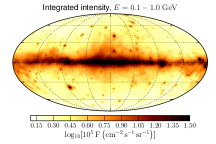
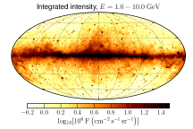
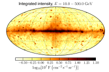
The observed gamma-ray emission can be divided into resolved point sources (PS) and diffuse emission. Most of the diffuse gamma-ray emission comes from interactions of CR nuclei with interstellar gas. Another important component of diffuse emission at high energies is due to IC emission from leptonic CRs interacting with the low-energy interstellar radiation field (ISRF). At energies below approximately 10 GeV, bremsstrahlung emission from electrons and positrons interacting with interstellar gas is important as well. These three components have a characteristic distribution on the sky that peaks near the Galactic plane. An additional isotropic gamma-ray component is made of several contributions, including residual CR contamination, unresolved extragalactic point sources, and extragalactic diffuse background.
Another diffuse emission component is represented by Loop I, a giant radio loop spanning on the sky (Large et al., 1962), which is also visible in the gamma-ray sky (Casandjian & Grenier, 2009). The origin of Loop I is an open question. It could be of local origin, produced either by a nearby supernova explosion or by the wind activity of the Scorpio-Centaurus OB association at a distance of 170 pc (Wolleben, 2007). Alternatively, it could be interpreted as a large-scale outflow from the Galactic center (Kataoka et al., 2013). In this paper we consider Loop I only as a foreground for the bubbles. A dedicated study of this feature is beyond the scope of this paper and left for future work.
The hadronic, IC, bremsstrahlung, isotropic and Loop I components comprise the most important emission components for an analysis of additional large scale gamma-ray structures, such as the Fermi bubbles. The general analysis strategy in the evaluation of the gamma-ray emission from the Fermi bubbles in this paper can be divided into the following steps:
-
1.
Construct a foreground emission model that includes known components555Note that the diffuse model provided by the Fermi-LAT collaboration through the Fermi Science Support Center cannot be used in this analysis, because it was developed for studies of point-like and small objects and, in particular, it already includes a simple model for the Fermi bubbles., namely point sources, hadronic emission from interactions of CR nuclei and ions with interstellar gas, IC emission and bremsstrahlung from CR electrons, isotropic emission and emission from Loop I (Section 3).
-
2.
Use the residual maps obtained by fitting and subtracting the known components from the data to find a template for the Fermi bubbles (Section 3.2).
-
3.
Find the spectrum of the Fermi bubbles using the template derived in the previous step together with the templates for the other components (Section 3.3).
3 Characterization of the Fermi bubbles using GALPROP templates
In this section we use the GALPROP package v54.1 to generate templates for the Galactic IC emission component and for the hadronic and the bremsstrahlung gamma-ray components. The latter ones are correlated with the distribution of interstellar gas. In the following, these components will be referred to as “gas-correlated”. GALPROP calculates the propagation and interaction of CRs in the Galaxy by numerically solving the diffusion equation for a specified model of the CR source distribution, a CR injection spectrum, and a model of the transport in the Galaxy. Parameters of the model are constrained by reproducing CR observables, including CR secondary abundances and spectra obtained from direct measurements in the solar system, and diffuse gamma-ray and synchrotron emission. We assume diffusive reacceleration with a Kolmogorov spectrum of interstellar turbulence and no convection. The diffusion coefficient is assumed to be isotropic. In the current version of GALPROP, all calculations assume azimuthal symmetry of the CR density with respect to the GC. Surveys of the 21-cm line of H I and the 2.6-mm line of CO (a tracer of H2) are used to evaluate the distribution of the target gas. The model of the ionized gas is based on observations of the pulsar dispersion measures and H emission (Gaensler et al., 2008). Dust maps are used to correct for the dark gas distribution that refers to neutral interstellar gas unaccounted for by the H I and CO surveys (Grenier et al., 2005; Ackermann et al., 2012).
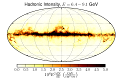
From the GALPROP calculation, we obtain gamma-ray emissivities corresponding to bremsstrahlung, and hadronic interactions with neutral (H I), ionized (H II), and molecular (H2) hydrogen in different Galactocentric rings, and IC emission. Since the bremsstrahlung is correlated with the distribution of gas, it is combined with the template of gamma rays from hadronic interactions. In the following, we also combine H I and H II rings, while we keep H2 rings independent. The gamma-ray intensity is proportional to a product of the gas and CR densities. The integral CR density is not well constrained a priori. To reduce the uncertainty related to the CR density, we use the gas-correlated templates in Galactocentric rings. The local ring template (r8–10 kpc from the Galactic center) for H I accounts for the vast majority of the gamma rays at latitudes , and therefore its normalization is kept free in the fit while we fix the other rings. The molecular hydrogen gas is mainly concentrated in isolated clouds at low latitudes. Since this contribution is small at high latitudes compared to the atomic hydrogen contribution, it is fixed in the fit. An IC template is created that takes into account the anisotropy of the ISRF due to an anisotropic flux of photons from the Galactic plane666We correct for the anisotropy of the cross-section by multiplying the generated IC maps with a map of the ratio between the predicted IC emission from a full anisotropic calculation, and the prediction assuming an isotropic cross-section (Ackermann et al., 2014).. Examples of hadronic and IC templates are shown in Figure 2. A detailed study of different GALPROP models and comparisons with Fermi LAT data is presented in Ackermann et al. (2012). For this paper, we consider a subset of models used in Ackermann et al. (2012) with updated H I gas maps. Compared to the gas maps used in Ackermann et al. (2012), the maps used here exclude the large and small Magellanic clouds, M31, and M33 as well as the Magellanic Stream and other high velocity clouds. The choice of a specific GALPROP model is a possible source of systematic uncertainties in our results. We address the question of systematic uncertainties in Section 3.3.
The following parameters describe our baseline GALPROP model777GALDEF file: galdef_54_Lorimer_z10kpc_R20kpc_Ts100000K_EBV5mag: the CR population is traced by the measured pulsar distribution (Lorimer et al., 2006), the CR confinement volume has a height of 10 kpc and a radius of 20 kpc, and H I column densities are derived from the 21-cm line intensities in the approximation of an optically thin medium, which is formally modeled by setting the spin temperature to 100,000 K.
The emission of Loop I is not modeled by GALPROP. It is a very important contribution because it overlaps the bubbles, especially in the Northern Galactic hemisphere (see Figure 1). Here we use two different approaches to model the emission of Loop I. In the first approach (used for the baseline model), we take a large elliptical region from the Haslam et al. (1982) map at 408 MHz around the Galactic center as a template of Loop I (Figure 2, bottom right). This approach is based on the assumption that the features in the Haslam map are produced by the synchrotron radiation from the same population of electrons that emit IC gamma rays. As an alternative way to model Loop I we use a geometric template based on a polarization survey at 1.4 GHz (Wolleben, 2007). The geometric Loop I model assumes synchrotron emission from two shells. Each shell is described by 5 parameters: the center coordinates , ; the distance to the center ; and the inner () and outer () radius of the shell. The parameters are set to: , , pc, pc, pc, , , pc, pc, pc (Figure 2, bottom left). Due to line of sight integration, the two uniform intensity spherical shells appear non-uniform with diffuse edges. The geometric Loop I template is included in the derivation of the systematic uncertainties (see Section 3.3). An isotropic template accounts for the extragalactic diffuse emission and the residual CR contamination.
A template for the bubbles is defined from the residual maps in Section 3.2. In the definition of the templates of the bubbles, point sources from the 2FGL catalog (Nolan et al., 2012) with a test statistic are masked with a radius of , which corresponds to the containment region of the PSF at 1 GeV. The test statistic is defined as TS = 2 , where is the likelihood. TS corresponds to a significance of just over . The twelve extended sources in the 2FGL catalog are masked conservatively within a circle of radius equal to the sum of the major semiaxis of the source template and the PSF containment radius. The source mask is displayed in Figure 3 on the right. Since the definition of the bubbles relies only on an analysis at high energies ( GeV), where the PSF core is narrow (), the masked point sources cover about of the area of the bubbles at . The spectrum of the bubbles is calculated over a broad energy range extending from MeV to GeV. The broad PSF at low energies does not allow sufficient masking of the sources without masking much of the area of the bubbles, and therefore requires a more accurate modeling. Since the 2FGL catalog was obtained with only 2 years of data and this analysis uses more than 4 years, we fit 472 bright point sources in the 2FGL catalog with TS using the full 50 months data set in order to account for flares happening outside of the time window of the 2FGL analysis. For each source, we fit the normalization in each energy bin. The remaining less significant sources are merged into a single template with fluxes from the 2FGL catalog. The overall normalization of this template is free in the fit. Individual sources fainter than the 2FGL limit are effectively part of the isotropic background. Their effect on the overall fit would be in the isotropic component and they would not impact the results for the bubbles.
The templates listed above are fit to the data (see Table 1 for a summary of the templates used in the derivation of the spectra). The fit is performed in each energy bin individually, i.e., if a template is kept free in the fit, its normalization in each energy bin is a free parameter in the fit.
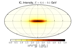
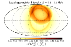
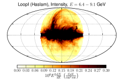
| Template | Description |
|---|---|
| Neutral and ionized atomic hydrogen | GALPROP: bremsstrahlung and hadronic production |
| (sum of H I and H II) | local ring: 8 - 10 kpc (free) |
| non-local component: 0 - 8 kpc and 10 - 50 kpc (fixed) | |
| Molecular hydrogen (H2) | GALPROP: bremsstrahlung and hadronic production |
| all Galactocentric rings combined (fixed) | |
| Inverse Compton radiation | GALPROP (free) |
| Bright 2FGL sources | , 472 sources: each fitted individually |
| Weak 2FGL sources | one template obtained by adding 2FGL fluxes (free) |
| Isotropic | extragalactic diffuse and |
| residual CR contamination (free) | |
| Loop I | Haslam map or geometric template (free) |
| Bubble | template obtained from residuals (Section 3.2) (free) |
3.1 Fitting algorithm
In order to extract the Fermi bubbles’ morphology and spectrum from the Fermi LAT data we use the all-sky fitting tool GaDGET (Ackermann et al., 2008), which simultaneously fits the different components of the diffuse Galactic emission to the Fermi LAT data in a maximum likelihood procedure based on Poisson statistics. MINUIT (James & Roos, 1975) was used as the optimizer with a tolerance of .
The model is a linear combination of templates
| (1) |
where is the template of the component in energy bin and in pixel . Coefficients are the fitting parameters. The model maps, which are in flux units, are multiplied with the exposure and convolved with the instrument PSF to obtain the corresponding count maps for comparison with the data count maps.
3.2 Defining a template for the Fermi Bubbles
In order to define a template for the Fermi bubbles, we perform an all-sky fit with the templates listed above except, of course, a template of the bubbles. We define the template of the bubbles based on the residuals at energies above GeV where the flux of the bubbles becomes readily apparent888Between 5 and 10 GeV the bubbles become clearly visible in the residuals and the exact choice of the threshold does not affect the results.. Since no template accounts for the bubbles’ flux, the coefficients of the fit will partially compensate for it, introducing a bias. To avoid this bias we mask an elliptical region that approximately covers the Fermi bubbles (Figure 3 on the left). Point sources are also masked (see above for details). The PS mask is shown in Figure 3 on the right. In the resulting residual map, the masked pixels are filled with the average of the neighboring not-masked pixels.
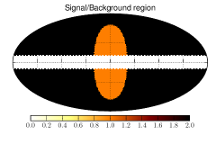
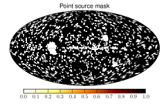
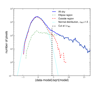
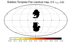
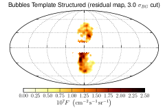
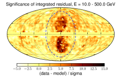
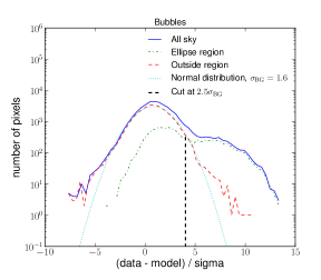
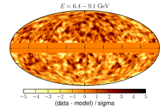
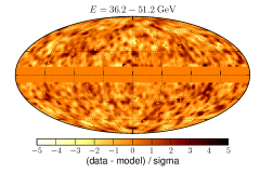
The significance map of the residuals (defined as (datamodel)/) for the baseline model defined in Section 3 integrated over energies is shown in Figure 4 (left). The template of the bubbles is determined by applying a threshold in the smoothed significance map. To find the threshold, we create a histogram (Figure 4, right) with the smoothed significance in each pixel in the region of interest and outside the region of interest (orange and black respectively in Figure 3, left). We consider the outside region as the background region and fit a Gaussian to the histogram. The width of the Gaussian is denoted as . The threshold in the definition of the template of the bubbles is set to . The results for a different threshold of are included in the systematic uncertainties (see Section 3.3). Figure 5 shows the resulting templates of the bubbles. We distinguish between flat and structured templates. In the flat template the value is 1 if the significance of the residual is more than the threshold and 0 otherwise, while the structured template is equal to the residual flux if the significance of the residual is greater than the threshold and 0 otherwise. In the baseline model, the bubbles are modeled with a structured template created with a significance threshold of .
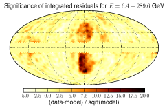
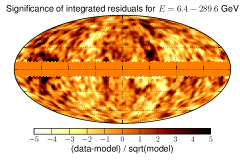
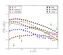
In the next step the template of the bubbles is included in the all-sky fit. This time, since no PS mask is applied, the point sources are included in the fit and not masked as in the derivation of the Fermi bubbles’ template. The integrated residual map after including the structured template of the bubbles in the fit and fitting the point sources is shown in Figure 6 (left). The spectra for the different components are presented in Figure 6 (right).
In the rest of the paper, the model of the foreground emission components and the Fermi bubbles presented in this section will be referred to as the baseline model.
3.3 Systematic uncertainties
To estimate the systematic uncertainties in the spectrum of the Fermi bubbles due to uncertainty in the modeling of the diffuse foregrounds and the bubbles, we study the variation of our results when using different GALPROP configurations and definitions of the templates of Loop I and the bubbles.
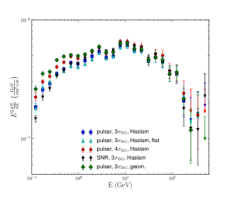
We tested two different tracers of the CR source distributions: the measured distribution of supernova remnants (SNR) (Case & Bhattacharya, 1998) and the measured pulsar distribution (Lorimer et al., 2006). In addition, we varied the size of the CR confinement volume. In GALPROP, the diffusion zone is a cylinder with radius and height above the Galactic plane. kpc and kpc and and 10 kpc have been tested. Furthermore, two different spin temperature values ( K and K) are used to correct for the H I opacity in order to derive the H I column density. K corresponds to the optically thin approximation. Loop I is either modeled by the Haslam map or by the geometric template. We also use a flat template of the bubbles instead of the structured template and vary the significance threshold used to define the bubbles ( and ). Figure 7 shows some examples of the bubbles’ spectra for different parameters of the model. Each case represents the change of one parameter relative to the baseline model configuration.
The all-sky fit and the extraction of the bubble spectrum was repeated with the different GALPROP configurations, Loop I models, and templates for the bubbles. The envelope of all tested models defines the systematic error band. The final result is shown in Section 5 where it is also compared to the spectrum obtained from the local template analysis (Section 4).
4 Characterization of the bubbles using local templates analysis
In this section we present an alternative approach for modeling the Galactic foreground emission which does not rely on the GALPROP modeling of CR propagation and interactions in the Milky Way. For example, one of the assumptions in the analysis presented in Section 3 is that the CR spectrum is independent of the azimuthal direction from the Galactic center. In general, this assumption may be violated, e.g., in the spiral arms. In this section, we relax this assumption by fitting templates in small regions on the sky (in the following called patches). Instead of using the gamma-ray emission maps provided by GALPROP, we directly use gas maps to trace the intensities of gamma-ray emission: H I and CO surveys uncorrected for absorption and dark gas (for a description see Ackermann et al., 2012) together with the Schlegel, Finkbeiner and Davis (SFD) dust map (Schlegel et al., 1998) to account for gas not traced by the H I or CO lines. The IC component is modeled by a bivariate Gaussian; the parameters of the Gaussians are found from fitting the model to the data (more details in Section 4.2).
Models for the gamma-ray emission components are derived one at a time. We start with the component with the brightest integrated flux, namely the gas-correlated emission. After that we subtract the gas-correlated emission from the data and define a template for the IC emission together with the isotropic component. Then we additionally subtract the IC and the isotropic components and determine the Loop I and the bubbles’ templates from the residuals. At each step the components that have not yet been determined are represented by proxy templates in order to avoid a bias in the fluxes. In the end, all templates are fit to the data simultaneously to determine the spectrum of the emission components.
In this analysis, we subtract the 2FGL point sources from the data using the 2FGL fluxes. In addition we mask the cores of the bright point sources with fluxes above 1 GeV greater than (556 sources) within , which corresponds to the 68% radius of the PSF at approximately 700 MeV. We test the influence of point sources on the determination of the spectrum of the Fermi bubbles by refitting the point sources with TS 200 to take into account flaring outside the 2FGL time window in Section 4.4.
4.1 Gas-correlated components via local template fitting
Gamma-ray intensities from a given direction that arise from hadronic interactions and bremsstrahlung are proportional to the column density of gas. The normalization coefficient is the emissivity, which can be given in terms of the gamma-ray emission rate per atom. In this section, we assume that in a limited region of the high-latitude sky (dubbed hereafter a patch), the CR density is approximately constant. In this case, we can determine the emissivity directly as the proportionality constant between gas column densities and gamma-ray intensities from a fit to the data in each patch of the sky.
The other emission components, i.e., IC, isotropic, Loop I, and the Fermi-bubbles, have to be modeled simultaneously with the gas-correlated component. Otherwise the gas-correlated contribution may be overestimated. We assume that the other components either are sufficiently smooth, or have features uncorrelated with the gas distribution, so that they can be modeled by a combination of some smooth functions in each patch. We choose two-dimensional polynomials defined locally on each patch as a linear basis for the smooth functions (determined below).
In order to avoid sharp edges for the patches, which may lead to artificial features in the residuals, we use a hyperbolic tangent function to obtain patches with smooth boundaries. The all-sky data and model maps are restricted to the patch by multiplication with the following weight function:
| (2) |
where is the angle from the center of the patch to the center of pixel , the radius of the patch is and the width of the boundary is . This function smoothly interpolates between for and for , where the width of the edge is assumed to be much smaller than the patch radius, i.e., . In Figure 8 we show an example of a patch with a gas template and a local polynomial template multiplied with the weight function.
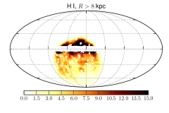
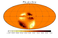
In the analysis, we separate the sky into 24 patches. Each patch has a radius and a edge width. There are 16 patches centered at and at , where . There are 8 patches centered at and at , where . The radius of the patches is chosen to be rather large so that the template fitting procedure converges well. The centers of the patches are chosen to cover the sky approximately uniformly with a significant overlap among the patches.
The data in each patch are modeled by a combination of gas templates and a combination of local polynomials up to a maximal degree which is determined in each patch from the convergence of the fit (more details below). The model in the patch is
| (3) |
where labels the energy bins, labels the pixels in the patch, labels the polynomials, and labels the gas templates, . In this analysis, we use four gas templates: H I summed over Galactocentric rings with kpc, H I summed over rings with kpc, summed over all rings, and the SFD dust template (Schlegel et al., 1998). We neglect the contribution from ionized hydrogen (H II) in this analysis. (If the corresponding contribution is smooth, it becomes a part of the local polynomial term). The scaling coefficient is proportional to the emissivity, corresponding to template as fitted in patch . Some of the patches at high latitudes may have little contribution from some gas templates, such as H I in the inner Galaxy rings or . The template is included in the fit if the “scalar product” between the template and the weight function that determines the patch is sufficiently large: where the norm is defined as the square root of the sum of the map values squared. The total number of gas templates in each patch is .
The second term in the model describes components that are not correlated with the gas distribution (isotropic, IC, Loop I, bubbles). These components are modeled by a combination of polynomials in local coordinates on the patch. We define the local polynomials on the sphere by taking a polynomial function on the plane tangent to the center of the patch and projecting the values of the function from the plane to the sphere using a stereographic projection. In terms of local coordinates and on the tangent plane, the polynomials are . If is the maximal degree, then the total number of polynomials is . The maximal degree of the polynomials depends on the position of the patch and on the energy range. We specify at the end of this section in the discussion of the stability of the fit.
In order to speed up the calculation, we use the quadratic approximation to the log likelihood, which for all-sky fits takes the form
| (4) |
where and are the number of gamma rays in the data and the model prediction for energy bin in pixel . We use the smoothed counts map as an estimator for the standard deviation , where the smoothing radius depends on energy bin . For each energy bin, the radius is chosen such that there are on average at least 100 photons inside the circle of radius . The minimal value of the radius is , which corresponds to an average over about 15 pixels. As we discuss in Appendix A, the choices or result in biased fitting, while reduces the bias.
The data fitting in a local patch is performed with the following weighted
| (5) |
Notice that the weighted is equivalent to a multiplication of the data and the model with the weight (without changing ). The best-fit parameters and, hence, the model depend on the patch. In this part of the analysis we mask which is different from the Galactic plane mask adopted in the rest of the paper. The reason is that the regions closer to the Galactic plane have more features in the gas maps, especially for the inner Galaxy H I template and the H2 template. Including these regions improves the convergence of the fits.
We use different fitting strategies at low and high energies. At low energies (0.1 - 10 GeV), the statistics are high and the normalization of the templates can be determined in every energy bin independently. At high energies the statistics are low. In order to avoid high statistical fluctuations among the energy bins, we assume that a single power law is a good approximation for the gas-correlated emission and find the best-fit power-law index for the energy bins between 3 and 500 GeV. In the intermediate region, i.e., between 3 and 10 GeV, we take the mean of the spectra. The best-fit combinations of polynomial templates are determined independently in each patch and in each energy bin both at low and at high energies.
The resulting contribution of the gas-correlated components depends on the degree of the polynomials used to model the other components. If the degree of the polynomial is too small, then the contribution of gas-correlated components will be overestimated due to absorption of the flux from the other components. For imperfect gas templates, a large degree of the polynomials leads to more of the gas-correlated gamma-ray emission being attributed to the polynomial templates. For a sufficiently high degree, the polynomial templates will start to respond to the noise, thus, over-fitting the data. Different portions of the sky require a different maximal degree of the polynomials. Near the Galactic plane and close to local features, such as the Fermi bubbles, the degree should be larger than at high latitudes, where the isotropic and the local IC emission can be described by smoother templates.
In the following we describe the determination of the maximal degree of the polynomials for a particular patch. The convergence of is not a good indicator: the value decreases with larger degree polynomials as more and more features are included in the model, but it does not reach the level of statistical noise up until a very high degree, where we are already likely to include some of the gas-correlated emission into the local polynomials. One of the characteristics of a good model of gas-correlated emission is the stability of the corresponding spectrum as the degree increases: we stop increasing the degree of the polynomials when the differences between the photon spectra of the gas-correlated component become smaller than a certain threshold. In particular, we calculate the difference of the spectra between and , i.e., we compare the last spectrum with the previous two spectra
| (6) |
where is the gas-correlated intensity for in an energy bin derived with the maximal degree of polynomials , is the statistical uncertainty of . At energies below 10 GeV, we use the threshold . This is much larger than the expected random fluctuations, but at low energies the differences are dominated by the systematic uncertainties and this level gives a good fit in Monte Carlo simulations. At energies above 3 GeV, the stability condition is , which is comparable to the statistical noise. In each case, if the stability condition is not satisfied, we stop at a maximal degree of 12, which corresponds to an angular scale of about .
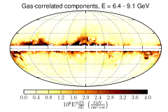
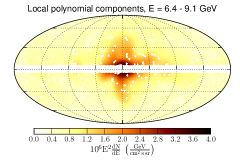
In each energy bin, all-sky models are obtained as a weighted average of the models in the patches
| (7) |
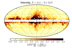
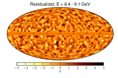
An example of gamma-ray counts, template maps and residuals is presented in Figure 9. Sharp features uncorrelated with the gas templates remain in the residual map in Figure 9, e.g., the left edge of the southern bubble. In the following, we use the weighted sum of the gas-correlated components as an all-sky template to determine the templates and the spectrum of the other components.
4.2 IC and isotropic components
The next step is to model the IC and isotropic components. First, we subtract the point sources and the gas-correlated component found in the previous subsection from the data. Examples of the polynomial models and the residuals after subtraction of the gas-correlated components are shown in Figures 9 and 10. One can notice the presence of two distinct components: a component along the Galactic disk (mostly IC) and a halo component (mostly Loop I and the Fermi bubbles).
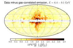
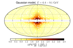
We model both the disk and the halo components by bivariate Gaussians with parameters and and and respectively. The centers of the Gaussians are fixed at the GC. We fit the two Gaussians together with the isotropic template to the residuals obtained by subtracting the gas-correlated emission components and the point sources from the data. The Gaussian for the halo is a proxy template for the bubbles and Loop I, and is necessary to avoid a bias in the determination of the disk template. The parameters of the Gaussians are fitted independently in each energy bin below 30 GeV. At higher energies, the parameters of the Gaussians are determined from a fit to the flux integrated above 30 GeV. The Gaussian model in the energy bin GeV is shown in Figure 10. In this section and below, we use the global fitting procedure described in Equation (4) without the additional weight factors introduced for the local templates analysis in Equation (5), i.e., we perform an all-sky fit instead of the local fit in patches.
4.3 Bubbles and Loop I
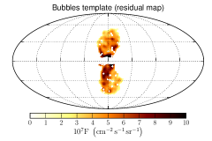
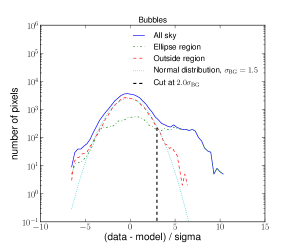
We define the template of the bubbles from the residual flux after subtracting the gas-correlated, isotropic, and disk components from the data. We do not subtract the halo component, which only served as a proxy for bubbles and Loop I in the previous step. The template for the bubbles is derived from the residual flux integrated above 10 GeV (Figure 11). Compared to the derivation of the template of the bubbles in Section 3.2, here we use the energy range above 10 GeV to test the uncertainty related to the choice of the lower energy bound (compared to 6.4 GeV in Section 3.2). The histogram of pixel counts inside and outside of the bubbles’ region and the template of the bubbles are shown in Figure 12. For the energy range above 10 GeV the pixel counts in the background region intersect the distribution of pixel counts in the ellipse region around , which we use in the definition of the template of the bubbles.
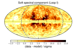
In order to separate Loop I from the Fermi bubbles, we determine these templates from a correlation with the spectra of the two components between 0.7 GeV and 10 GeV, where the contribution from both Loop I and the bubbles is significant. The energy range is chosen to be relatively small so that the spectra are well approximated by a simple power-law function.
The derivation of templates correlated with the known spectra is similar to the derivation of the spectra for known templates. If we represent the residuals after subtracting the gas-correlated, IC, and isotropic components in energy bins and in pixels as a matrix , then, assuming that we can neglect the statistical uncertainty, the problem of separating this residual into components is equivalent to the following matrix separation problem (e.g., Malyshev, 2012)
| (8) |
where is a matrix of the spectra and is an matrix of templates. If the spectra are known, then the corresponding templates are determined as
| (9) |
This solution also works in the case of uniform statistical uncertainties. In the case of a non-uniform uncertainties, one has to minimize the
| (10) |
The only effect of this more general derivation is an inclusion of a factor in all sums over energy bins and over pixels in Equation (9).
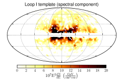
We assume that the residuals between 0.7 GeV and 10 GeV are dominated by two components: hard and soft components corresponding to the bubbles and Loop I respectively. We estimate the spectrum of the soft component from residuals outside of the region of the Fermi bubbles: and . A power-law fit in this region has a photon index . The spectrum of the hard component is determined from the residuals near the southern edge of the Fermi bubbles: and . A power-law fit in this region has a photon index . Thus, to determine the Loop I template we use , while for the template of the bubbles we use . The corresponding hard and soft components are shown in Figure 13. To check the systematic uncertainty, we vary the indices in the definitions of the templates in Section 4.4.
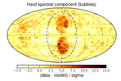
The templates in Equation 9 can be written as a linear combination of the residual maps
| (11) |
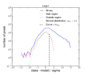
where labels the energy bins, labels the pixels, and labels the emission components (Loop I and the bubbles). are linear decomposition coefficients. The cuts are relative to the standard deviation outside of the regions containing the bubbles and Loop I. The standard deviation of the linear combinations of maps in Equation (11) is the root mean square of the standard deviations of the terms in the linear combination
| (12) |
where is the statistical uncertainty of the data in energy bin in pixel (derived from the square root of the observed photon counts). The templates of the bubbles and Loop I are derived by applying threshold cuts of and to the spectral components maps, which are chosen from the comparison of the background pixel counts to the pixel counts in the Loop I and the bubbles regions (Figure 14). We note that both methods considered in this work give comparable results for the template of the Fermi bubbles (Figures 5, 12, 14).
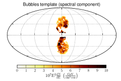
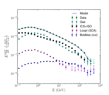
The spectra obtained by fitting the five templates (gas-correlated, isotropic, IC, bubbles, and Loop I) to the gamma-ray data for are shown in Figure 15. Let us summarize the characteristics of this model as it will be used as a reference model in the study of the systematic uncertainties in the next subsection. We use the 2FGL spectra for point sources, the local patches have a radius of , gas-correlated components are modeled by a combination of H I gas templates in two rings, the H2 template, and the SFD dust template, the spectrum of the gas-correlated components at high energies is a power law, the template of the bubbles is obtained from the residual above 10 GeV, while the Loop I template is obtained with the spectral components analysis method. We use structured flux templates for the bubbles and Loop I. The significance of the residuals for this fit is presented in Figure 16.
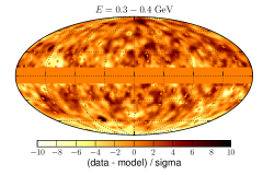
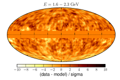
4.4 Systematic uncertainties
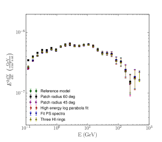
In order to estimate the systematic uncertainties in the local templates analysis, we take the model presented in the previous subsection and vary some aspects of the fitting procedure. At first, we vary the parameters relevant to the derivation of the Galactic emission components (Figure 17 on the left):
-
1.
We try different patch radii in the determination of the gas-correlated components: and .
-
2.
To test the dependence on the assumption of a power-law spectrum for the gas-correlated emission at high energy, we use a log parabola function to model the gas-correlated spectra at high energies999This test is motivated by possible deviations from a simple power law in the gamma-ray spectrum due to features in the hadronic CR spectra (Adriani et al., 2011b). The log parabola function is the simplest generalization of a power law..
-
3.
We also try to use three H I rings (R 8 kpc, 8 kpc R 10 kpc, and 10 kpc R, see Table 1) as opposed to 2 rings (R 8 kpc and 8 kpc R).
-
4.
To test the dependence on the model of the point sources, we refit bright point sources with (472 sources). We keep the positions given in the 2FGL catalog and refit the spectra of the point sources assuming the same spectral function (e.g., power law, power law with a cutoff, or log parabola). The fit is performed in a small patch around each point source: the radius is either or the 95% containment angle, whichever is larger. This choice of the radius is motivated by the requirement that there are sufficiently many pixels to perform the fit, but not too many pixels, so that a low order polynomial model of the background is appropriate: the background is modeled by a combination of local polynomials of degree 4 (the degree was found from Monte Carlo tests). During a fit for a particular point source, all other 2FGL point sources with TS are subtracted from the data with the 2FGL fluxes.
-
5.
We also mask the cores of the point sources without subtracting them. This has a relatively important effect at low energies, where the PSF is large. But even in this case, the difference in the spectrum of the bubbles is not significant compared to the effect from modifying the definitions of the bubbles’ and Loop I templates considered below.
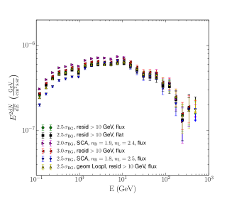
In order to test the systematic uncertainty related to the definition of the Fermi bubbles and the Loop I templates, we consider the following definitions of the templates (Figure 17 on the right):
-
1.
Bubbles’ template from residual maps above 10 GeV (we tested two threshold levels: 2.5 and 3).
-
2.
Bubbles’ template from spectral components with indices 1.9, 1.8 (2 and 2.5).
-
3.
Loop I template from spectral components with indices 2.4, 2.5 (1 and 1.2).
-
4.
Geometric Loop I template (Section 3).
-
5.
We use structured (proportional to flux) and flat (0 - 1) templates both for the bubbles and for Loop I.
The largest effect at low energies comes from the assumptions on the spectrum of the components in the spectral components analysis (SCA) derivation of the templates for the bubbles and for the Loop I.
5 The overall spectrum of the bubbles
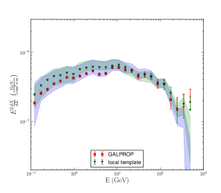
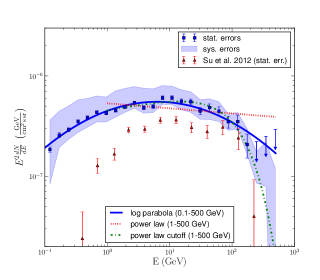
The spectra of the bubbles derived with the two methods presented in Sections 3 and 4 are shown in Figure 18, left. In the following, we take the results from the GALPROP template analysis as a baseline for the spectral energy distribution (SED) and combine all the spectra obtained with the two methods to get an envelope of the systematic uncertainties. The envelope includes uncertainties introduced by the diffuse modeling and uncertainties related to the analysis strategy, e.g., the threshold to define the template of the bubbles, or the size of the local patches. We add the systematic error of the LAT effective area (Ackermann et al., 2012) in quadrature to the envelope obtained for different models. The systematic errors of the LAT PSF and the effect of energy dispersion are negligible given the spatial and energy binning chosen for this analysis. The uncertainties due to the modeling of Galactic foregrounds and analysis strategy (see Table 2) dominate the uncertainty compared to the effective area, which has a relative flux error of . The baseline model with its statistical and systematic uncertainties is presented in Figure 18 on the right and in Table 2. We also compare our results with the Fermi bubbles’ SED derived by Su & Finkbeiner (2012). Our intensity is significantly higher than the spectrum of Su & Finkbeiner (2012), especially at low energies. The difference is due to a combination of several effects, namely a smaller Galactic plane mask ( in this work compared to in Su & Finkbeiner (2012)), a smaller area of the bubbles’ template in this analysis resulting in larger intensities, the inclusion of a separate template for the cocoon in Su & Finkbeiner (2012), and different modeling of the Galactic foregrounds. Our results agree with the spectrum in latitude strips at reported by Hooper & Slatyer (2013).
We fit the baseline SED with a log parabola function, a power law with an exponential cutoff and a simple power law (Figure 18, right). The log parabola and the power law with an exponential cutoff are defined, respectively, as
| (13) | |||||
| (14) |
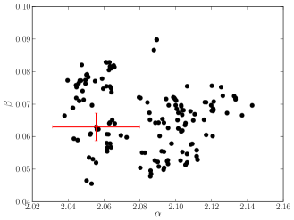
We repeat the fits for the bubbles’ spectrum for different Galactic models and different definitions of the bubbles and Loop I templates. We obtain the following parameters for the log-parabola function in the fit range 100 MeV to 500 GeV: , . The values are given for the baseline model and the systematic uncertainties are estimated from the SEDs obtained for different Galactic foreground models and choices in the analysis strategy. The systematic errors include the uncertainties of the LAT effective area Ackermann et al. (2012). The distributions of the fit parameters and for the log parabola fits are shown in Figure 19 on the left.
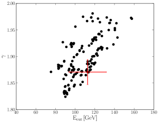
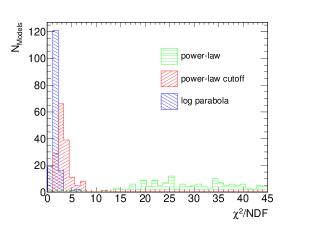
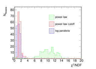
The power law with a cutoff fit above 100 MeV is dominated by low and intermediate energies. In order to find a value of the high-energy cutoff unbiased by low energies, we fit the power law with a cutoff in the range 1 GeV to 500 GeV. We obtain GeV and . The distribution of indices and cutoff energies of the power law with exponential cutoff fits are shown in Figure 19 on the right. The corresponding distributions of per number of degrees of freedom (NDF) are presented in Figure 20. The log parabola gives a good description of the data over the whole energy range. The simple power law does not describe the data well even above 1 GeV. The power law with a cutoff is preferred over a power law with at least 7 significance.
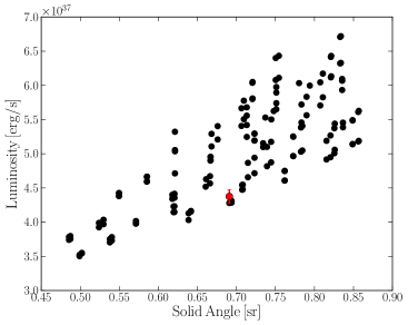
We calculate the total luminosity of the bubbles for for each determination of the spectrum in the energy range from 100 MeV to 500 GeV. The bubbles are found to have a luminosity of erg s-1. The distribution of the solid angle subtended by the bubbles, and the luminosity for the models considered are shown in Figure 21.
| [GeV] | ] | |||||
| 0.12 | 0.10 | 0.14 | 1.85 | 0.83 | 3.61 | 0.11 |
| 0.17 | 0.14 | 0.20 | 2.57 | 1.37 | 4.44 | 0.15 |
| 0.24 | 0.20 | 0.28 | 2.91 | 1.70 | 5.35 | 0.13 |
| 0.34 | 0.28 | 0.40 | 3.51 | 2.27 | 6.11 | 0.13 |
| 0.48 | 0.40 | 0.57 | 3.85 | 2.51 | 6.29 | 0.14 |
| 0.67 | 0.57 | 0.80 | 4.35 | 2.67 | 6.69 | 0.15 |
| 0.95 | 0.80 | 1.13 | 4.26 | 2.90 | 6.47 | 0.16 |
| 1.35 | 1.13 | 1.60 | 4.53 | 3.99 | 7.49 | 0.17 |
| 1.90 | 1.60 | 2.26 | 4.91 | 4.52 | 7.80 | 0.18 |
| 2.69 | 2.26 | 3.20 | 5.40 | 4.98 | 7.88 | 0.20 |
| 3.81 | 3.20 | 4.53 | 4.83 | 4.48 | 7.73 | 0.20 |
| 5.38 | 4.53 | 6.40 | 4.96 | 4.58 | 7.56 | 0.23 |
| 7.61 | 6.40 | 9.05 | 6.05 | 5.42 | 8.01 | 0.26 |
| 10.76 | 9.05 | 12.80 | 6.04 | 5.42 | 7.91 | 0.28 |
| 15.22 | 12.80 | 18.10 | 5.58 | 4.73 | 7.17 | 0.31 |
| 21.53 | 18.10 | 25.60 | 5.52 | 4.23 | 6.82 | 0.35 |
| 30.44 | 25.60 | 36.20 | 4.47 | 3.80 | 5.71 | 0.37 |
| 43.05 | 36.20 | 51.20 | 4.84 | 3.73 | 5.80 | 0.42 |
| 60.89 | 51.20 | 72.41 | 4.45 | 3.76 | 5.41 | 0.46 |
| 86.11 | 72.41 | 102.40 | 3.49 | 2.95 | 4.06 | 0.48 |
| 121.77 | 102.40 | 144.82 | 3.51 | 3.07 | 4.23 | 0.57 |
| 172.22 | 144.82 | 204.80 | 2.07 | 1.71 | 2.77 | 0.56 |
| 243.55 | 204.80 | 289.63 | 1.07 | 0.88 | 1.79 | 0.57 |
| 344.43 | 289.63 | 409.60 | 1.23 | 0.81 | 2.06 | 0.63 |
| 487.10 | 409.60 | 579.26 | 0.00 | 0.00 | 1.28 | 1.46 |
6 Morphology and spectral variations
The average spectrum of the bubbles is an important characteristic, but it may be insufficient for distinguishing among the models of the bubbles’ formation and the mechanisms of the gamma-ray emission. In this section, we calculate the spectrum of the bubbles in latitude strips, and estimate the significance and the spectrum of the enhanced gamma-ray emission in the south-eastern part of the bubbles, called the “cocoon” (Su & Finkbeiner, 2012). We search for a jet inside the bubbles and determine the location and the width of the boundary of the bubbles.
6.1 Longitude Profiles
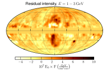
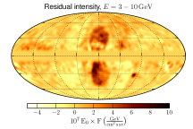
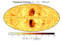
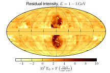
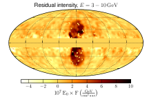
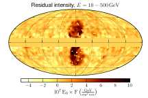
To give a general idea about the morphology of the bubbles, we present the profile plots of the residual intensity corresponding to the Fermi bubbles at different latitudes integrated in three energy bands: 1 - 3 GeV, 3 - 10 GeV, 10 - 500 GeV. The residual intensity is shown in Figure 22. There is an L-shaped over-subtraction at low energies in the GALPROP residuals in the low latitude part of the northern bubble. This residual is spatially correlated with the star forming region Ophiuchi, which might have a different CR spectrum compared to the average. Notice that this feature is not present in the residuals obtained from the local template analysis, which allows the adjustment of the normalization of the CR density in local patches. The profile plots in latitude strips are shown in Figure 23.
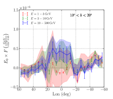
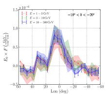
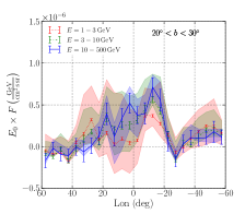
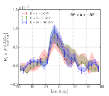
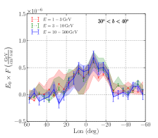
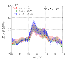
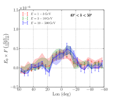
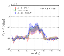
An excess of emission in the southern bubble for latitudes and longitudes corresponds to the cocoon proposed by Su & Finkbeiner (2012). There is also a slight excess of emission for around . At some latitudes, the width of the boundary of the bubbles is approximately or smaller than . We study the width of the edge in more detail in Section 6.3.
6.2 Substructures
In this section, we present an analysis of substructures within the bubbles. In the residual maps we find an enhanced gamma-ray emission mostly in the south east side of the Fermi bubbles. Following Su & Finkbeiner (2012), we will denote the region of enhanced gamma-ray emission as the “cocoon”, although the physical origin of this emission is not known. In order to study the significance and the spectrum of the cocoon, we separate the cocoon template from the bubbles and fit both the cocoon and the bubbles templates together with the other diffuse foreground templates to the data.
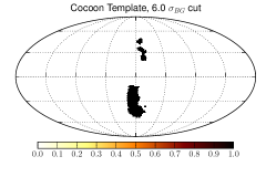
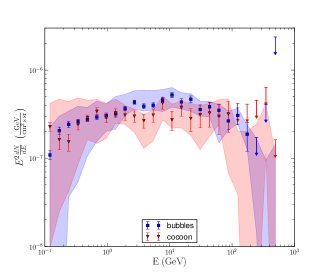
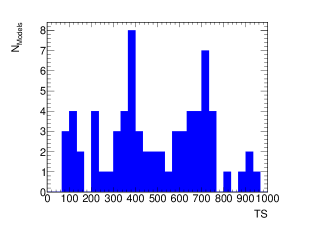
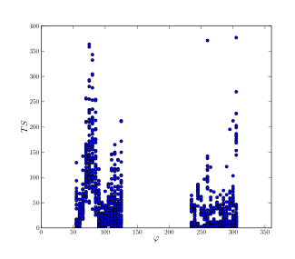
We derive the cocoon template from the same residual maps that we use for the derivation of the Fermi bubbles by applying a higher cut in significance. We take 6 in the GALPROP templates analysis and 5 in the local templates analysis. The difference is due to the difference in the energy ranges used to define the templates in the two methods (see Section 4.3). The cocoon template for the baseline model (defined in Section 3) is shown in Figure 24 (left). Notice that in contrast to the cocoon template in Su & Finkbeiner (2012) this template is not restricted to the southern hemisphere and includes also excess emission in the North. In the fits we use the flat template for the bubbles; otherwise the structures in the template of the bubbles can absorb a significant part of the cocoon emission. We also use a flat cocoon template to get a conservative estimate of the significance of the cocoon. Note that the cocoon template is inside the template of the bubbles, i.e., the cocoon emission is on top of the emission from the bubbles modeled by a flat template. Using both the cocoon and the bubbles’ templates improves the likelihood of the fit relative to the flat template for the bubbles alone. We find that TS is between 95 and 975, depending on the foreground emission model, while the number of additional free parameters in the fit is 25 (one for each energy bin). Figure 25 shows the distribution of TS for different foreground emission models. The probability that the cocoon is a statistical fluctuation is . This probability does not include the trials factor.
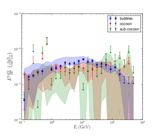
The intensity spectrum of the cocoon is compared to the spectrum of the bubbles in Figure 24 (right). We find that the spectrum of the cocoon is consistent with the spectrum of the rest of the bubbles. However, due to large statistical uncertainties in the cocoon spectrum we cannot rule out a simple power-law spectrum of the cocoon emission. The absolute value of intensity of the gamma-ray emission from the cocoon detected on top of the flat bubbles template is, by coincidence, very similar to the gamma-ray intensity of the bubbles. In other words, the intensity in the cocoon region is about two times larger than the intensity inside the bubbles but outside of the cocoon.
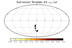
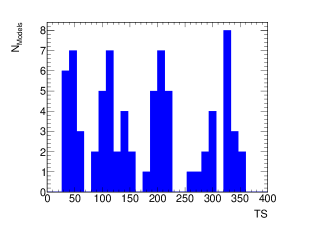
In a second step we apply an even higher significance threshold of 9 to the residual map. We call the resulting structure the “sub-cocoon”. The sub-cocoon template is displayed in Figure 26 (left). We include this template in the all-sky fit together with a flat bubbles and a flat cocoon template. The resulting spectra are shown in Figure 26 (right). The improvement of the fit obtained by including the additional template is displayed in Figure 27. We find that TS for different foreground models is between 30 and 360 (for 25 additional free parameters). The probability that the sub-cocoon is a statistical fluctuation is about considering the smallest TS value among all models.
In the following we investigate the existence of jet-like emission as proposed by Su & Finkbeiner (2012), who tentatively observed a pair of jets along the cocoon’s axis of symmetry with a harder spectral index compared to the spectrum of the bubbles. The existence of a jet within the bubbles would be an important indication of an AGN-like activity of the black hole in the Galactic center.
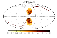
To test this hypothesis we use a generic jet template, which is a strip of width and length originating in the Galactic center. We rotate this template in steps. Note, that the physical distance corresponding to at is , i.e., the jets cover practically all pixels within from the GC. Figure 28 (left) shows an illustration of all jet templates. Note that we include only one jet template at a time in each fit. Because the emission of the sun could mimic a jet as the Sun moves along the ecliptic, which passes near the Galactic center, we also add a template for the gamma-ray emission from cosmic-ray interactions in the outer atmosphere and radiation field of the Sun101010A description of the solar template can be found at the Fermi Science Support Center: http://fermi.gsfc.nasa.gov/ssc/data/analysis/scitools/solar_template.html (Johannesson et al., 2013). For each position of the jet we calculate the improvement of the fit (compared to a fit with only flat bubbles and flat cocoon template). Figure 28 (right) shows the distribution of for the jet template in different orientations for different diffuse models. There is a broad enhancement towards several directions centered at , which cover the cocoon. In those cases, the jet templates account for some remaining excess emission on top of the cocoon, that is not modeled by the flat cocoon template. In summary, we do not find significant residuals aligned along a specific direction that could be interpreted as a jet.
6.3 Width of the boundary of the bubbles
The sharpness of the edge is one of the main arguments for a transient process of bubble formation (Su et al., 2010). The main difficulties in estimating the width of the edge are the statistical error and the systematic uncertainty due to modeling of the diffuse foreground gamma-ray emission. In order to get maximal information from the available data, we have chosen to perform a parametric fit of a smoothed step function (modeled by a hyperbolic tangent) across the edge of the bubbles. The algorithm has the following steps:
-
1.
Choose a reference point approximately on the bubble edge (by visual inspection of residuals above 10 GeV).
-
2.
Find the gradient of the residual by fitting a plane to the residual intensity in pixels within from the reference point. The gradient is along the direction of maximal change in the residual flux. We use it to define the direction perpendicular to the edge.
-
3.
In order to find the position of the edge and its width, we choose a strip along the gradient and project the data onto the gradient direction. This allows us to reduce the fitting to a one-dimensional fitting problem. We take the length of the strip to be ( from the reference point), and the width to be ( from the reference point). The size of the bins in the projection is , which is larger than the pixel size but small enough that resolving the sharp transitions is possible.
-
4.
Fit the data along the strip with a smoothed step function modeled by the hyperbolic tangent plus a constant:
(15) In total we have the four parameters A, , , and C. Two of them are non-linear ( and ). The best-fit position of the edge is determined by , the width of the edge is defined as , and the constant models the residual background emission. During the fit to the data, the model is convolved with the PSF for each energy range.
-
5.
Test the systematic uncertainty by changing the length and the width of the strip and the size of the bins. The lengths are , , , the widths are , , , and the bins are and wide.
-
6.
Test the systematic uncertainty related to the derivation of the foreground models and the templates of the bubbles and Loop I.
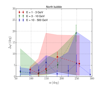
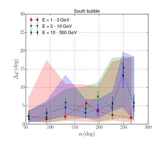
We derive the width of the bubbles’ edge in three energy ranges: 1 - 3 GeV, 3 - 10 GeV, 10 - 500 GeV. The average PSF is dominated by the events at the lower boundaries of the energy ranges. The 68% PSF containment angles at 1 GeV, 3 GeV, and 10 GeV are , , and respectively. Examples of fitting the hyperbolic tangent function across the bubble edge for the residual maps above 10 GeV are shown in Figure 29. In Figure 30 we show the location of the edge and the width overplotted on the residual map. A summary of the edge widths, including statistical and systematic uncertainties, is presented in Figure 31. The values are reported in Table 3. Sometimes the fit of the width does not converge, either due to oversubtractions in the foreground modeling or due to lack of statistical significance. In this table, we do not report values of the width larger than , which is comparable to the size of the bubbles themselves, or less than , which is smaller than the resolution of the pixelation. We find that in most locations along the bubbles edge, the width of the boundary varies between and . The value of in one location in the southern bubble is because the edge lies on top of a local excess (see Figure 30). This high value is likely due to poor convergence of the fit rather than the actual width of the boundary.
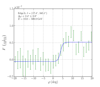
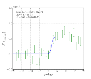
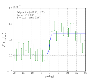
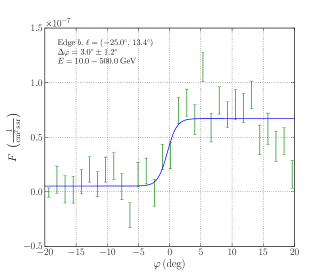
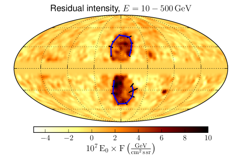
We do not detect a significant difference in the width of the bubbles’ boundary for the three energy ranges. The median width of the bubbles’ boundary among all locations along the boundary and among all models of foreground emission and templates of the bubbles is deg. The systematic uncertainty boundaries are estimated as values which enclose % of the values above and below the median value. We take the median instead of the mean in order to avoid bias due to outliers with large values of the width either due to oversubtractions in the foreground modeling or poor convergence of the width estimation.
| Lat | Lon | Width | Stat | Min Width | Max Width |
|---|---|---|---|---|---|
| North | |||||
| 17.4 | 345.1 | 2.4 | 2.0 | 0.9 | 4.0 |
| 25.5 | 342.0 | 1.7 | 1.3 | 0.7 | 3.4 |
| 35.3 | 339.1 | 2.9 | 1.5 | 2.0 | 6.3 |
| 44.8 | 342.5 | 6.3 | 2.5 | 1.2 | 9.4 |
| 47.7 | 3.1 | 1.2 | 1.5 | 0.7 | 5.3 |
| 37.5 | 14.9 | 2.5 | 2.4 | 0.5 | 10.6 |
| 30.0 | 18.3 | 5.8 | 3.8 | 0.6 | 19.8 |
| 16.8 | 16.8 | 0.9 | 2.2 | 0.5 | 15.7 |
| South | |||||
| -17.1 | 11.7 | 1.4 | 2.3 | 1.0 | 3.6 |
| -25.0 | 13.4 | 3.0 | 1.2 | 1.0 | 6.3 |
| -35.0 | 15.1 | 4.5 | 1.4 | 2.4 | 13.3 |
| -51.1 | 5.6 | 3.1 | 1.4 | 1.8 | 6.7 |
| -50.3 | 347.8 | 4.0 | 1.6 | 1.6 | 6.8 |
| -39.5 | 337.1 | 5.6 | 1.8 | 3.6 | 8.8 |
| -30.9 | 337.1 | 13.3 | 3.4 | 4.7 | 19.7 |
| -23.3 | 340.3 | 5.8 | 2.2 | 0.8 | 18.3 |
6.4 Spectrum in latitude strips
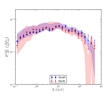
The spectra for northern and southern bubbles are shown in Figure 32. These spectra are derived similarly to the overall spectrum of the bubbles, but instead of one template of the bubbles, we fit two independent templates: for the northern and southern bubbles. We find that the spectra in the North and in the South agree with each other within the uncertainties. The southern bubbles has a region of enhanced emission, the cocoon, while the brightness in the northern bubbles is more uniform. The overall intensities of the two bubbles are consistent with each other.
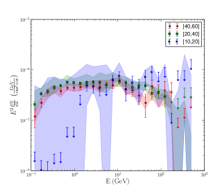
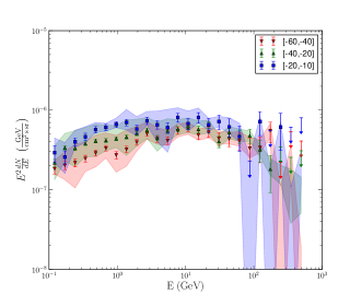
The spectra in latitude strips are shown in Figure 33. For the derivation of the spectra in strips we separated the template of the bubbles into 6 independent templates according to latitude. The latitude boundaries of the stripes are to , to and to in the South and to , to and to in the North. With the current level of statistical and systematic uncertainties, we cannot detect a variation of the spectrum with latitude. Our results agree with Hooper & Slatyer (2013) at latitudes , but we do not find a significant variation of the spectrum of the bubbles for compared to higher latitudes. There is a large systematic uncertainty in the energy spectrum at latitudes mostly due to uncertainties of the model of the foreground gamma-ray emission from the interactions of CR with interstellar gas. Manifestation of this uncertainty can be seen in the residual maps in Figure 22 and in the profile plots in Figure 23.
7 IC and hadronic models of the bubbles
In this section we fit the spectrum of the bubbles with IC and hadronic models of gamma-ray production. In addition, we calculate the synchrotron emission from the population of electrons in the IC model and from the secondary electrons and positrons in the hadronic model. The details of the calculations are presented in Appendix B.
7.1 IC model of the bubbles
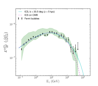
The IC scattering is calculated with the cross sections presented by Blumenthal & Gould (1970). The interstellar radiation field (ISRF) is taken from the GALPROP v54 distribution (Porter & Strong, 2005; Moskalenko et al., 2006). Since no significant variation of the gamma-ray spectrum across the bubbles has been found, we will use the spectrum averaged over the area of the bubbles (Figure 18, right, and Table 2).
As a benchmark model for the spectrum of electrons we take the spectrum derived using the ISRF at 5 kpc above the GC. We also compare it with the electron spectrum obtained for CMB photons only.
Since the gamma-ray spectrum of the Fermi bubbles has a significant cutoff at high energies, we model the electron spectrum by a power law with an exponential cutoff . The best fit parameters are and TeV. The corresponding IC spectra are shown in Figure 34 on the left. The details of the calculation can be found in Appendix B.1. The indices and the cutoff values for different foreground models and definitions of the templates of Loop I and the bubbles are shown in Figure 34 on the right. The bremsstrahlung emission is at least two orders of magnitude smaller than the IC emission for a characteristic gas density at a few kpc from the Galactic plane (Snowden et al., 1997), and can be neglected.
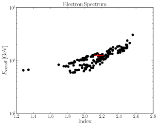
We will assume that the center of the bubbles is at , i.e., the distance to the center of the bubbles is kpc, where kpc is the distance to the GC. The total energy contained in the electron population inside the bubbles above 1 GeV is erg, where the value corresponds to the baseline model; the statistical uncertainty is calculated by marginalizing over the index and cutoff of the electron spectrum. The systematic uncertainty is estimated by calculating the electron spectrum for different models of the foreground emission and definitions of the templates of the bubbles and Loop I.
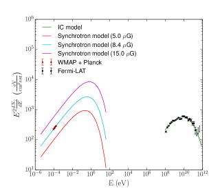
The synchrotron emission from the benchmark population of electrons for different values of the magnetic field is shown in Figure 35 together with the IC signal. On the same plot, we also include the Planck and WMAP microwave haze spectrum (Pietrobon et al., 2012; Ade et al., 2013). The index of the microwave haze emission is harder than the synchrotron emission for a stationary population of electrons in the Galaxy. The microwave haze spatially overlaps with the gamma-ray bubbles at . We confirm that the population of electrons that produces the gamma-ray emission of the Fermi bubbles via IC scattering can also produce the microwave haze (Dobler et al., 2010; Su et al., 2010; Su & Finkbeiner, 2012; Dobler, 2012; Ade et al., 2013).
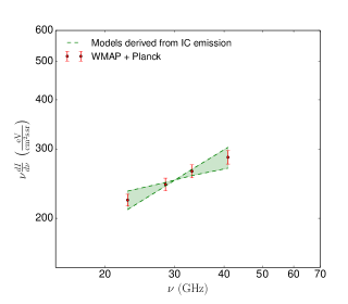
The range of spectra of the synchrotron emission corresponding to the systematic uncertainty in the electron spectrum (Figure 34) is shown in Figure 35 on the right. For each electron spectrum, we find the magnetic field that gives the best fit to the microwave data. We find , where the value is for the baseline model, the statistical uncertainty is calculated using the statistical errors of the WMAP and Planck haze spectra, the systematic uncertainty is due to modeling of the gamma-ray foregrounds and the definition of the template of the bubbles. The allowed magnetic fields are approximately in the range from 5 to 20 G. A larger index (softer spectrum) corresponds to a greater number density of electrons at lower energies; in this case the magnetic field is G. A harder index requires a magnetic field of G. The uncertainties of the index and magnetic field are due to large uncertainties in the distribution of electrons around GeV. We note that the spectrum of the microwave haze was obtained for latitudes (Pietrobon et al., 2012), i.e., the derived magnetic field corresponds to the region of the bubbles encompassed by these latitudes. At higher latitudes the microwave haze emission has smaller intensity, which can be explained if the magnetic field decreases with height above the Galactic plane.
The main contribution to the IC signal comes from electrons at energies GeV. We show in Appendix B that the main contribution to the WMAP and Planck frequencies, where the microwave haze is detected, comes from electrons between 10 GeV and 30 GeV. Thus, although the gamma-ray bubbles and the microwave haze can be produced by the same population of electrons, the presence of two populations of electrons cannot be excluded: one population producing the gamma-ray signal and the other producing the microwave signal. In this scenario, the magnetic field can have a lower value. As a result, the electron cooling time can be longer than in the case of a single population of electrons.
The cooling time for 1 TeV electrons in a 5 G magnetic field and in the ISRF at 5 kpc is only 500 kyr, while taking into account only the IC losses gives a cooling time of Myr (Appendix B.2). If the bubbles were formed by a jet or an outflow from the Galactic center, where most of the acceleration happened during the initial stages of the expansion, then the expansion velocity should be greater than 10,000 km/s so that the bubbles formation time is smaller than the cooling time of the 1 TeV electrons. The lower bound on the expansion velocity becomes 20,000 km/s, if the magnetic field is 5 G. In scenarios with electron reacceleration inside the volume of the bubbles (Mertsch & Sarkar, 2011), the characteristic acceleration time for 1 TeV electrons should be shorter than 1 Myr for IC losses only, or 500 kyr for IC and synchrotron losses in a 5 G magnetic field. Since the synchrotron losses at these energies are about the same as the IC losses, in the case of a steady injection, the electron injection rate should be about two times larger than the gamma-ray luminosity of the bubbles, i.e. around .
7.2 Hadronic model of the bubbles
For the calculation of the spectrum of gamma rays produced in hadronic interactions, we use the cross sections described in Kamae et al. (2006) and Karlsson & Kamae (2008), which are implemented in the cparamlib package111111https://github.com/niklask/cparamlib. In this analysis, we consider only proton cosmic rays in the hadronic model of the gamma-ray emission in the bubbles. We parameterize the spectrum of the protons as a function of momentum. A power law with an exponential cutoff spectrum of the CR protons
| (16) |
gives a better fit at high energies than a simple power-law spectrum (Figure 36). The parameters of the power law with a cutoff function are and . In order to estimate the amount of energy in hadronic cosmic rays required to produce the gamma-ray signal, one needs to know the density of gas inside the bubbles. We take into account only ionized hydrogen and we use as a reference value for the density121212Note, that the gamma-ray emissivity integrated along the line of sight, which is relevant for the template fitting, is dominated by H I from the local ring, while the emissivity a few kpc above the Galactic plane is dominated by ionized hydrogen.. It is of the same order of magnitude as the plasma density at 2 kpc above the Galactic center (Snowden et al., 1997).
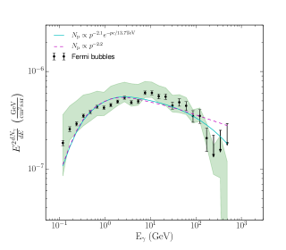
The total energy in hadronic CRs above 1 GeV required to produce the gamma rays is . Including heavier nuclei may change this estimate. However, the evaluation of this effect depends on the uncertain composition of CRs and gas in the bubbles, hence it is beyond the scope of the modeling in this paper. In the relevant energy range of the proton kinetic energy 0.1 - 10 TeV, the center of mass energy is 10 - 100 GeV and the inelastic cross section is . The average time for a collision is . In a steady state, the minimal injection rate of cosmic-ray protons is . This calculation assumes that the main energy loss process is inelastic proton-proton collisions. The injection rate actually required may be an order of magnitude higher due to, e.g., adiabatic losses.
The proton spectrum at high energies inside the bubbles must be much harder than the spectrum of CR protons in the Galactic plane (e.g., Adriani et al., 2011b; Ackermann et al., 2012; Dermer et al., 2013). If we assume that the proton spectrum injected in the ISM by the supernova explosions is the same everywhere in the Galaxy and is , then the softening of the spectrum in the Galactic plane can be explained by energy-dependent escape, while the hard proton spectrum inside the bubbles can be explained if the escape time from the bubbles is longer than the interaction time (Crocker & Aharonian, 2011). In other words, protons escape from the Galactic plane before they interact, but the protons inside the bubbles should interact before they can escape, which means that they have to remain inside the bubbles for several Gyr.
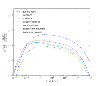
In addition to producing gamma rays, interactions of high-energy protons also produce electrons, positrons, and several species of neutrinos. The flux of neutrinos from the hadronic interactions in the Fermi bubbles has been previously considered by Lunardini & Razzaque (2012); Adrián-Martínez et al. (2013); Ahlers & Murase (2013); Lunardini et al. (2013). We present our calculation of the fluxes of all particles produced in the hadronic interactions in Figure 37 on the left. As above, in this calculation the cross sections are taken from the cparamlib package. The electrons and positrons are included in this plot only formally to show their relative production cross sections compared to the cross sections of neutrinos and gamma rays. In reality, the secondary leptons are assumed to be trapped inside the bubbles together with the protons. Note that we calculate the neutrino spectrum based on the average gamma-ray spectrum of the bubbles. However, we cannot rule out that the cocoon spectrum follows a simple power law, which might produce neutrinos at higher energies.
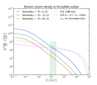
We now calculate the synchrotron emission from the secondary produced in the hadronic collisions inside the bubbles. The secondary electrons and positrons undergo cooling due to IC and synchrotron losses. We denote the energy loss function as , where for the synchrotron and the IC energy loss in the Thomson approximation (Appendix B). Assuming that the high-energy leptons lose their energy inside the bubbles, the stationary energy density of secondary electrons and positrons is
| (17) |
where is the spectrum of electrons or positrons produced in interactions of hadronic CR with interstellar gas. We compare the energy density of secondary to the energy density of electrons necessary to produce the gamma-ray flux of the bubbles by IC scattering in Figure 37 on the right.
In the range of energies relevant for the WMAP and Planck haze, the density of the secondary electrons and positrons is comparable to the electrons producing the IC. Above the pion cutoff at MeV, the injection spectrum for the secondary leptons is proportional to the proton spectrum . There is an additional softening by one power of due to cooling. As a result, the spectrum of the secondary leptons above 100 MeV is proportional to .
Below the pion cutoff, the spectrum of secondary leptons is harder than and the integral in Equation 17 is insensitive to the lower energy bound. As a result, the stationary spectrum of the secondary leptons below 100 MeV is simply proportional to . For the benchmark gas density , the bremsstrahlung emission from the secondary leptons is at least an order of magnitude smaller than the gamma-ray signal for all energies above 100 MeV and we neglect it in our analysis.
The IC and synchrotron spectra from the secondary leptons produced in the hadronic model for different magnetic fields are shown in Figure 38 on the left. We note that the synchrotron intensity is a factor of 3 - 4 lower than the WMAP and Planck points and one cannot correct for this offset by tuning the magnetic field. The reason is that for electrons with a spectrum the synchrotron radiation scales as , but for large magnetic field strengthes the synchrotron energy losses dominate and the normalization of the secondary electrons is proportional to . Consequently the dependence on the magnetic field cancels out. This is the reason that the synchrotron intensity is saturated for . The IC flux is proportional to the stationary energy density of the secondary leptons and it decreases with increasing magnetic field.
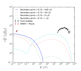
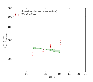
The synchrotron radiation produced by electrons is which is significantly softer than the microwave haze spectrum (Ade et al., 2013). The distribution of indices for the synchrotron radiation from the secondary leptons is shown in Figure 38 on the right. The lines on this plot are obtained by calculating the synchrotron radiation from the secondary leptons in a 10 G magnetic field with a subsequent rescaling (for illustration) by an overall normalization factor to fit the WMAP and Planck points.
The range of indices and the renormalization factors that we use to rescale the synchrotron radiation from the secondary leptons to fit the microwave haze are shown in Figure 39. Both the index and the rescaling factor have a relatively small range of values because both the leptons around 10 GeV, which are responsible for the synchrotron radiation, and the gamma rays around 10 GeV, where the Fermi bubbles spectrum has small statistical and systematic errors, are produced by the same protons with energies around 100 GeV. As a result, the synchrotron radiation at WMAP and Planck haze frequencies is directly linked to the gamma-ray radiation around 10 GeV in this scenario. The conclusion is that there should be either an additional source of primary electrons or a reacceleration of the secondary leptons inside the bubbles to increase the overall normalization by a factor of 3 and to produce the spectrum of electrons and positrons around 10 GeV required to fit the microwave haze data. The timescale of this reacceleration should be smaller than the cooling time of electrons around 10 GeV, which is about 10 Myr for a 10 G magnetic field (Appendix B.2). Another possibility in the hadronic scenario of the Fermi bubbles is transporting the electrons from the Galactic plane in the wind from supernovae together with the hadronic CR (Crocker & Aharonian, 2011). The timescale of 10 Myr is sufficient to bring the electrons to 10 kpc above the Galactic plane with a wind of about 1000 km s-1. These electrons can produce the microwave haze by synchrotron radiation. They may also contribute to the gamma-ray spectrum at energies GeV by IC scattering off starlight.
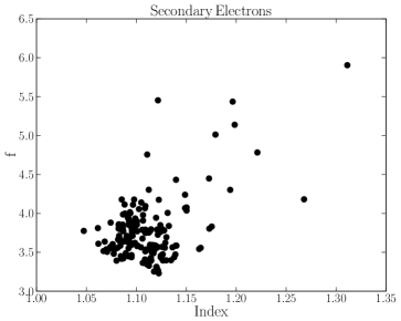
Including emission from secondary leptons (Equation 17) in the hadronic models can improve the fit. The secondary gamma-ray spectrum depends on the value of the magnetic field: for magnetic fields larger than approximately 5 G, most of the power injected in secondary leptons is dissipated into synchrotron emission and the gamma-ray spectrum is similar to the primary only emission. The total primary and secondary gamma-ray spectrum for a 2 G magnetic field is shown in Figure 40 on the left. A sample of proton spectral indices and cutoffs for the energy spectra of the Fermi bubbles derived for different foreground models and definitions of the bubbles and Loop I templates is shown in Figure 40 on the right.
In Figure 41 we compare the reduced for IC and hadronic models of the Fermi bubbles. In general, we find that the IC models fit the spectrum of the bubbles better than the primary gamma-ray spectrum in hadronic models with a significance of at least (Figure 41 left). The distribution of the difference between the in leptonic and hadronic models including secondary emission is presented in Figure 41 on the right. For some cases, the hadronic model including secondary gamma-ray emission has a comparable to the IC model. Therefore, we cannot discriminate between hadronic and IC models based on the current gamma-ray data alone. This calculation does not include uncertainties in the nuclear production models, which could affect the gamma-ray spectrum at low energies up to (Dermer, 2012)131313Note that the microwave haze is produced by electrons at energies above 10 GeV, where the uncertainties in the nuclear production cross sections are lower (Dermer, 2012), hence, they are subordinate to the systematic uncertainties related to modeling of the foreground diffuse emission..
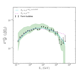
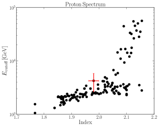
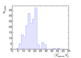
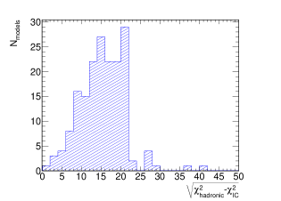
8 Summary and conclusions
In this paper, we analyze 50 months of Fermi-LAT data in order to determine the morphology and the spectrum of the Fermi bubbles. The main challenge is the spatial overlap with the other components of diffuse gamma-ray emission due to collisions of hadronic CRs with the interstellar gas, IC production of gamma rays, bremsstrahlung, extragalactic gamma-ray emission, and contamination from CRs.
We model the foreground gamma-ray emission with two independent methods. In the first method we use maps generated by the GALPROP CR propagation and interaction code as templates of the emission components. Fitting these templates to the data makes this method less sensitive to the distribution of CR sources and to the propagation model. In the second method we develop a more general data-driven model of diffuse gamma-ray foregrounds. We use gas maps derived from the 21-cm, CO, and dust surveys as tracers of the gamma rays produced by interactions of hadronic CRs and by bremsstrahlung. We fit the gas-correlated templates on small patches of the sky together with a combination of 2D polynomial functions that model components of emission not correlated with the distribution of the gas. In this method no assumptions are made on CR sources or propagation, except for an assumption that the CR density inside each patch can be approximated by a constant. After subtracting the gas-correlated component from the data, we model the IC component as a bivariate Gaussian along the Galactic plane.
One of the largest systematic uncertainties is the definition of the template for Loop I, which is a large structure in the sky, overlapping the Fermi bubbles mostly in the northern hemisphere. In the paper we use three different definitions of the Loop I template: a template based on the radio data at 408 MHz (Haslam et al., 1982), a geometrical model based on the 1.4 GHz polarization data (Wolleben, 2007), and a template derived from the gamma-ray residuals based on a correlation with the gamma-ray spectrum in the residuals outside the Fermi bubbles. We determine templates for the bubbles from the residuals obtained after subtracting the foreground emission components.
We find that the gamma-ray spectra of the Fermi bubbles derived with the two methods agree with each other. At energies above approximately 10 GeV the uncertainty in the spectrum is dominated by statistics while below 10 GeV systematic uncertainties are dominant. The total luminosity of the bubbles between 100 MeV and 500 GeV is erg s-1 (assuming that they are located at the distance of the Galactic center). The spectrum of the bubbles is well described either by a log parabola function or by a power law with an exponential cutoff. The fit of the photon spectrum above 1 GeV by a power law with an exponential cutoff has an index and a cutoff GeV. A simple power-law spectrum is excluded with very high confidence (Figure 20). Both the log parabola and a power law with an exponential cutoff fit the spectrum of the Fermi bubbles with for some models of gamma-ray diffuse foregrounds and the definition of the bubbles and Loop I templates. In the energy range between 100 MeV and 500 GeV, a log parabola gives a slightly better fit than a power law with a cutoff. The reported spectrum has a higher normalization and a softer spectrum at energies below 1 GeV compared to previous results (Su & Finkbeiner, 2012). For the first time we show that a significant cutoff exists at high energies.
The brightness of the emission is not uniform across the bubbles: we confirm the previously reported (Su & Finkbeiner, 2012) excess of emission on the south-eastern side of the bubbles (referred to as the cocoon). We define a template for the cocoon similarly to the bubbles template by applying a higher cut in significance to the residual maps. We find that fitting a flat cocoon template together with a flat bubbles template improves the fit compared to the flat bubbles template case by for NDF = 25 (Figure 25). The probability that the cocoon is a statistical fluctuation is for some models of foreground emission that we have tested and for all definitions of the bubbles and Loop I templates. The energy spectrum of the cocoon is consistent with the spectrum of the Fermi bubbles.
We search for a jet-like structure inside the bubbles using two different techniques. First, we apply a higher cut in the residual significance map than in the definition of the cocoon (Figure 26). This structure is not significant, with a probability of statistical fluctuation of for all models of foreground emission. We also searched for a narrow linear feature emanating from the Galactic center (Figure 28). We do not find any significant linear jet (in contrast to tentative claims by Su & Finkbeiner, 2012) within our systematic uncertainty, although the scatter in significance for the different foreground models is very high.
The spectra of the northern bubble and the southern bubble are consistent with each other (Figure 32). We find no variation of the spectrum with latitude within the statistical and systematic uncertainties in contrast to claims by Hooper & Slatyer (2013) and Yang et al. (2014). The systematic uncertainties are especially high for the strips in the North due to strong contamination from gamma rays produced in hadronic interactions and a significant overlap with Loop I.
We estimate the position and the width of the boundary of the bubbles by fitting a hyperbolic tangent function across the edge of the bubbles. The width is calculated for residuals in three energy ranges: 1 - 3 GeV, 3 - 10 GeV, and 10 - 500 GeV. We find that, on average, the width is smaller than . We do not find a significant variation of the width with energy but the width changes with position along the boundary of the bubbles (Figure 30).
We fit the spatially integrated spectrum of the bubbles with IC and hadronic models of gamma-ray production. The spectrum of the electrons in the IC model is well described by a power law with an exponential cutoff with and and the total energy in electrons above 1 GeV is erg. The spectrum of the protons in the hadronic scenario is expressed as a function of the proton momentum with and . The total energy in proton CRs above 1 GeV is . The IC model fits the energy spectrum of the Fermi bubbles better than the primary gamma-ray emission in the hadronic model with a significance of at least without taking into account the uncertainties in the nuclear cross sections of Kamae et al. (2006). If we include gamma-ray emission from secondary leptons and assume a magnetic field weaker than approximately 5 G, then the quality of the fits of the hadronic models to the gamma-ray data becomes comparable to the IC models (Figure 40). The derived spectra of CRs in leptonic and hadronic models of the Fermi bubbles agree with the previous results (e.g., Crocker & Aharonian, 2011; Mertsch & Sarkar, 2011).
For IC models of the bubbles, the homogeneous energy spectrum within the area of the bubbles and the rather sharp edges may favor a transient bubble formation scenario with either fast transport of leptonic CRs to high latitudes or continuous reacceleration of leptons within the volume of the bubbles. The cutoff in the energy spectrum can be explained by cooling of electrons due to IC and synchrotron energy losses. The presence of a cutoff in the proton spectrum for the hadronic model of gamma-ray production (Crocker & Aharonian, 2011) would indicate that either the mechanism of proton acceleration becomes less efficient around a few TeV or that the protons with higher energies can escape from the bubbles.
We find that the electrons in the IC scenario can also explain the WMAP and Planck microwave haze data for a magnetic field in the range between 5 G and 20 G (Figure 35). The secondary electrons and positrons in the hadronic scenario produce synchrotron radiation with a spectrum that is too soft compared to the microwave haze spectrum while the overall normalization of the synchrotron radiation from the secondary particles is at least a factor 3 - 4 smaller than the microwave haze level (Figures 38 and 39). A simultaneous explanation of the gamma-ray and the microwave data in a hadronic model requires an additional source of primary electrons or a reacceleration of the secondary leptons.
9 Acknowledgements
The Fermi-LAT Collaboration acknowledges generous ongoing support from a number of agencies and institutes that have supported both the development and the operation of the LAT as well as scientific data analysis. These include the National Aeronautics and Space Administration and the Department of Energy in the United States, the Commissariat à l’Energie Atomique and the Centre National de la Recherche Scientifique / Institut National de Physique Nucléaire et de Physique des Particules in France, the Agenzia Spaziale Italiana and the Istituto Nazionale di Fisica Nucleare in Italy, the Ministry of Education, Culture, Sports, Science and Technology (MEXT), High Energy Accelerator Research Organization (KEK) and Japan Aerospace Exploration Agency (JAXA) in Japan, and the K. A. Wallenberg Foundation, the Swedish Research Council and the Swedish National Space Board in Sweden.
Additional support for science analysis during the operations phase is gratefully acknowledged from the Istituto Nazionale di Astrofisica in Italy and the Centre National d’Études Spatiales in France. Some parts of the data analysis have been done with the HEALPix package (Gorski et al., 2005).
Appendix A approximation to the likelihood
In Section 4, we use the quadratic approximation to the log likelihood
| (A1) |
where is the gamma-ray data and is the model in an energy bin and a pixel . For a large number of counts the statistical uncertainty in the denominator is . For both choices and the fit has a statistically significant bias. For example, consider an energy bin (in the following argument we omit the energy index for brevity). If the underlying distribution of photons is isotropic (for example, in a high latitude patch), then the best estimate of the model is the arithmetic mean . If, however, one takes , then the minimization gives the harmonic mean
| (A2) |
The reason for this bias is that the fluctuations above the true model are underweighted in the , while the fluctuations below the true model are overweighted.
In the second case, if we take and minimize with respect to , then we get the quadratic mean
| (A3) |
The reason for this bias is that models with larger have smaller due to the presence of in the denominator.
In order to get an unbiased from a minimization, one can take . In this case both the best-fit parameter and the standard deviation found from the minimization coincide with the best estimators in the true Poisson distribution. Indeed, the estimators of the mean and the standard deviation of the mean in a Poisson distribution are
| (A4) |
The same values are obtained by minimizing
| (A5) |
with respect to . In particular, the standard deviation of the mean is
| (A6) |
The observed gamma-ray flux is not uniform, i.e., we cannot average over the whole sky to get an estimate of . The gamma-ray flux can be approximated as a constant only locally. We find the value of the local average by smoothing the data with a Gaussian kernel. At low energies the radius of the kernel is , which corresponds to averaging over approximately 15 pixels in the pixelation scheme chosen for the paper. At energies where on average there are fewer than 100 photons within a radius we take the smoothing radius such that there are on average 100 photons within . The radius stays at up to 5 GeV, then it grows to about at 100 GeV, and at 500 GeV. Thus the estimate of the that we use in the definition is given by the smoothed counts map , where the smoothing radius depends on energy bin . There is still a small bias due to using the smoothed data counts instead of the true but unknown model. This bias manifests itself in a small underestimation of the total gamma-ray flux. The difference is less than 1% below 2 GeV, it increases up to 2 - 3% around 10 GeV, and above 10 GeV it is smaller than the statistical uncertainty. This bias is much smaller than the other sources of the systematic uncertainty.
Appendix B IC and hadronic models of the bubbles
Here we present details about the calculation of IC and hadronic gamma-ray emission to model the spectrum of the Fermi bubbles. As in Section 7, we use the baseline model in Figure 18 as an example of the gamma-ray spectrum of the bubbles, while the other determinations of the Fermi bubbles spectra are used to estimate the systematic uncertainties.
B.1 IC model of the Fermi bubbles
The IC emission is produced by the scattering of high energy electrons on the ISRF photons. The density of the ISRF photons (Porter & Strong, 2005; Moskalenko et al., 2006) that we use to calculate the IC emission is presented in Figure 42 on the left. The three large bumps (going from left to right) correspond to CMB, IR, and starlight (SL) photons. In this analysis we use the ISRF distribution at kpc.
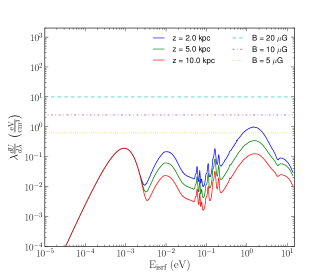
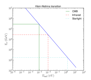
The energy spectrum of the IC photons is found from the convolution of the electron and the ISRF densities
| (B1) |
where is the speed of light, is in units of , and and are in units of . For completeness we present the scattering cross section (Blumenthal & Gould, 1970)
| (B2) |
where is the Thomson cross section and
| (B3) |
The transition between the non-relativistic (Thomson) and relativistic (Klein-Nishina) scattering happens when the energy of the ISRF photon in the center of mass is comparable to the mass of the electron . The maxima of the CMB, IR and starlight components of the ISRF at 5 kpc are , and . The characteristic electron energies for the maxima of the ISRF components are shown in Figure 42 on the left. For starlight photons the Klein-Nishina transition is around 100 GeV.
The gamma-ray flux is determined from the source energy density as a line of sight integral
| (B4) |
If we assume a spatially uniform ISRF distribution, then the flux of gamma rays can be expressed in terms of the column density of the electrons
| (B5) |
Then
| (B6) |
The best-fit electron spectrum is in units of . The total energy in electrons above 1 GeV is
| (B7) |
where is the surface area of the bubbles (for ) and kpc is the distance to the center of the bubbles at .
The contribution of different ISRF fields and the contribution of electrons of different energies to the gamma-ray flux is presented in Figure 43. Most of the contribution below 100 GeV comes from the CMB, which is the most abundant source of photons in terms of the number density. Above 100 GeV the IC signal is dominated by starlight and IR photons. In this calculation, we assume isotropic IC scattering cross section. The anisotropy of the starlight and IR photon flux at high latitudes may introduce a correction to the calculations (Moskalenko & Strong, 2000) at energies above 100 GeV where the IR and starlight contribution is significant. The magnitude of the change is not expected to be large as one can see from Figure 34, where we compare the full ISRF model with CMB only IC emission.
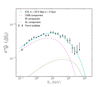
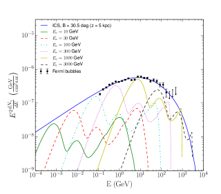
B.2 Microwave haze
In this subsection, we calculate the synchrotron emission from the same population of electrons derived in the previous subsection. We find that this population of electrons can also explain the WMAP and Planck microwave haze data (Finkbeiner, 2004; Ade et al., 2013).
The power emitted by an electron with an energy in a magnetic field with an angle between the electron velocity and the magnetic field is (Blumenthal & Gould, 1970)
| (B8) |
where is the modified Bessel function of the second kind and is the critical frequency
| (B9) |
The electron distribution can be expressed as a product of a distribution related to pitch angle , , and the energy spectrum
| (B10) |
The power emitted from a volume element is
| (B11) |
The intensity of microwave flux is derived analogously to Equations (B4) and (B6)
| (B12) |
where is the same distribution of electrons as in Equation (B5). We assume that there is no dependence on the pitch angle, i.e., .
In Figure (44) on the left we show the contribution of electrons at different energies to the total synchrotron spectrum. The curves are derived from Equation (B12) by integrating only over the pitch angle . For a given electron energy , most of the emitted power is concentrated around the critical frequency. In Figure (44) on the right we show the critical frequency for a range of magnetic fields relevant to the problem (we assume on this plot). The electrons at energies between 5 and 30 GeV contribute most of the power in the synchrotron emission at the WMAP and Planck frequencies. From Figure 43 we find that most of the contribution to the gamma-ray emission of the bubbles comes from electrons with energies above 100 GeV, i.e. the gamma-ray spectrum of the Fermi bubbles and the microwave haze signal in WMAP and Planck data are produced by electrons in different energy ranges.
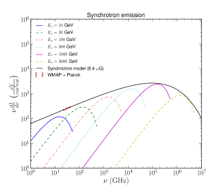
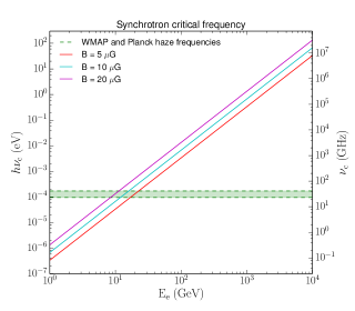
In Figure 45 we show the cooling time for electrons in different magnetic fields. In the case of zero magnetic field, all energy losses in this figure are due to IC scattering. The starlight photons do not contribute significantly to the energy loss above 100 GeV. Above 100 TeV the IR and the CMB photons must be considered in the Klein-Nishina regime as well. As a result, the IC cooling time above 100 TeV is leveling out (top curve on the left plot).
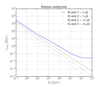
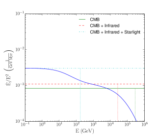
B.3 Hadronic model of the Fermi bubbles
The gamma rays can be produced as a result of an interaction of high energy CR protons with interstellar gas. The rate of gamma-ray production per unit volume and unit energy is
| (B13) |
where and are the densities of CR protons and hydrogen atoms per unit volume, is the velocity of the CR, and is the differential cross section to produce a gamma ray with energy in an interaction of a CR proton with kinetic energy and the nucleus of a hydrogen atom at rest.
We assume that the hadronic CR spectrum can be described as a power law in momentum at low energies. The derivative with respect to is transformed to the derivative with respect to the momentum through the expression
| (B14) |
The gamma-ray flux at the in the vicinity of Earth is
| (B15) |
where we assume a constant gas density throughout the bubbles and denote the line of sight integral of the CR density as
| (B16) |
In Figure 46 we show examples of fitting the gamma-ray data assuming a power law or a power law with a cutoff form of . We also show the contribution from different proton momenta in the power law with an exponential cutoff case. The parameters are . In order to find the normalization and the total energy in protons, we need to make an assumption on the number density of hydrogen atoms inside the bubbles. We take as a reference value.
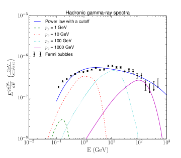
The source function for the secondary particles is
| (B17) |
where denotes the particle species. The flux of neutrinos can be calculated similarly to the flux of gamma rays in Equation (B15)
| (B18) |
The flux of neutrinos from the bubbles was presented in Figure 37 on the left.
We compare the CR energy density in leptonic and hadronic models to the energy density of a 8.4 G magnetic field in Figure 47. We find that the energy density of CR in hadronic model of the Fermi bubbles is approximately in equipartition with the magnetic field. In IC model of the Fermi bubbles the energy density in leptonic CR is much lower than the magnetic field energy density.
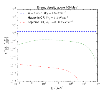
In Figure 48 we compare the CR energy density in leptonic and hadronic models of the Fermi bubbles to the local CR energy density. In hadronic model of the bubbles, the energy density of CR is about an order of magnitude larger than the energy density of local CR. In the leptonic model, the energy density of leptonic CR inside the bubbles is comparable to the local energy density of leptonic CR. The spectrum of leptonic CR in the bubbles is harder. As a result, above (below) 100 GeV the spectrum of leptonic CR inside the bubbles is larger (smaller) than the local CR spectrum.
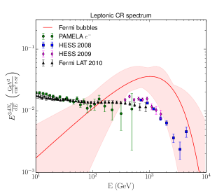
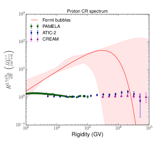
References
- Ackermann et al. (2012) Ackermann, M., Ajello, M., Albert, et al. 2012, ApJS, 203, 4
- Ackermann et al. (2010) Ackermann, M., Ajello, M., Atwood, et al. 2010, Phys. Rev. D, 82, 092004
- Ackermann et al. (2012) Ackermann, M., Ajello, M., Atwood, W. B., et al. 2012, Astrophys.J., 750, 3
- Ackermann et al. (2014) Ackermann, M., Albert, A., Atwood, W. B., et al. 2014, submitted to ApJ
- Ackermann et al. (2008) Ackermann, M., Jóhannesson, G., Digel, S., et al. 2008, in American Institute of Physics Conference Series, Vol. 1085, American Institute of Physics Conference Series, ed. F. A. Aharonian, W. Hofmann, & F. Rieger, 763–766
- Ade et al. (2013) Ade, P. A. R., Aghanim, N., Arnaud, M., et al. 2013, A&A, 554, A139
- Adrián-Martínez et al. (2013) Adrián-Martínez, S., Albert, A., Samarai, I. A., et al. 2013, ArXiv:1308.5260
- Adriani et al. (2011a) Adriani, O., Barbarino, G. C., Bazilevskaya, G. A., et al. 2011a, Physical Review Letters, 106, 201101
- Adriani et al. (2011b) —. 2011b, Science, 332, 69
- Aharonian et al. (2009) Aharonian, F., Akhperjanian, A. G., Anton, G., et al. 2009, A&A, 508, 561
- Aharonian et al. (2008) Aharonian, F., Akhperjanian, A. G., Barres de Almeida, U., et al. 2008, Physical Review Letters, 101, 261104
- Ahlers & Murase (2013) Ahlers, M., & Murase, K. 2013, ArXiv:1309.4077
- Atwood et al. (2009) Atwood, W. B., Abdo, A. A., Ackermann, M., et al. 2009, ApJ, 697, 1071
- Bland-Hawthorn et al. (2013) Bland-Hawthorn, J., Maloney, P. R., Sutherland, R. S., et al. 2013, ApJ, 778, 58
- Blumenthal & Gould (1970) Blumenthal, G. R., & Gould, R. J. 1970, Reviews of Modern Physics, 42, 237
- Carretti et al. (2013) Carretti, E., Crocker, R. M., Staveley-Smith, L., et al. 2013, Nature, 493, 66
- Casandjian & Grenier (2009) Casandjian, J.-M., & Grenier, I. 2009, arXiv:0912.3478
- Case & Bhattacharya (1998) Case, G. L., & Bhattacharya, D. 1998, Astrophys.J., 504, 761
- Cheng et al. (2011) Cheng, K.-S., Chernyshov, D. O., Dogiel, V. A., et al. 2011, ApJ, 731, L17
- Crocker & Aharonian (2011) Crocker, R. M., & Aharonian, F. 2011, Physical Review Letters, 106, 101102
- Dermer (2012) Dermer, C. D. 2012, Physical Review Letters, 109, 091101
- Dermer et al. (2013) Dermer, C. D., Finke, J. D., Murphy, R. J., et al. 2013, ArXiv:1303.6482
- Dobler (2012) Dobler, G. 2012, ApJ, 750, 17
- Dobler et al. (2010) Dobler, G., Finkbeiner, D. P., Cholis, I., et al. 2010, ApJ, 717, 825
- Finkbeiner (2004) Finkbeiner, D. P. 2004, ApJ, 614, 186
- Gaensler et al. (2008) Gaensler, B. M., Madsen, G. J., Chatterjee, S., et al. 2008, PASA, 25, 184
- Gorski et al. (2005) Gorski, K., Hivon, E., Banday, A., et al. 2005, Astrophys.J., 622, 759
- Grenier et al. (2005) Grenier, I. A., Casandjian, J.-M., & Terrier, R. 2005, Science, 307, 1292
- Guo & Mathews (2012) Guo, F., & Mathews, W. G. 2012, ApJ, 756, 181
- Guo et al. (2012) Guo, F., Mathews, W. G., Dobler, G., et al. 2012, ApJ, 756, 182
- Haslam et al. (1982) Haslam, C., Salter, C., Stoffel, H., et al. 1982, Astron.Astrophys.Suppl.Ser., 47, 1
- Hooper & Slatyer (2013) Hooper, D., & Slatyer, T. R. 2013, Phys.Dark Univ., 2, 118
- James & Roos (1975) James, F., & Roos, M. 1975, Comput.Phys.Commun., 10, 343
- Johannesson et al. (2013) Johannesson, G., Orlando, E., & for the Fermi-LAT collaboration. 2013, ArXiv:1307.0197
- Jones et al. (2012) Jones, D. I., Crocker, R. M., Reich, W., et al. 2012, ApJ, 747, L12
- Kamae et al. (2006) Kamae, T., Karlsson, N., Mizuno, T., et al. 2006, ApJ, 647, 692
- Karlsson & Kamae (2008) Karlsson, N., & Kamae, T. 2008, ApJ, 674, 278
- Kataoka et al. (2013) Kataoka, J., Tahara, M., Totani, T., et al. 2013, ApJ, 779, 57
- Large et al. (1962) Large, M. I., Quigley, M. J. S., & Haslam, C. G. T. 1962, MNRAS, 124, 405
- Lorimer et al. (2006) Lorimer, D., Faulkner, A., Lyne, A., et al. 2006, Mon.Not.Roy.Astron.Soc., 372, 777
- Lunardini & Razzaque (2012) Lunardini, C., & Razzaque, S. 2012, Physical Review Letters, 108, 221102
- Lunardini et al. (2013) Lunardini, C., Razzaque, S., Theodoseau, K. T., et al. 2013, ArXiv:1311.7188
- Malyshev (2012) Malyshev, D. 2012, ArXiv:1202.1034
- Mertsch & Sarkar (2011) Mertsch, P., & Sarkar, S. 2011, Physical Review Letters, 107, 091101
- Moskalenko & Strong (1998) Moskalenko, I., & Strong, A. 1998, Astrophys.J., 493, 694
- Moskalenko et al. (2006) Moskalenko, I. V., Porter, T. A., & Strong, A. W. 2006, ApJ, 640, L155
- Moskalenko & Strong (2000) Moskalenko, I. V., & Strong, A. W. 2000, ApJ, 528, 357
- Nolan et al. (2012) Nolan, P. L., Abdo, A. A., Ackermann, M., et al. 2012, ApJS, 199, 31
- Panov et al. (2006) Panov, A. D., Adams, J. H., Ahn, H. S., et al. 2006, ArXiv:0612377
- Pietrobon et al. (2012) Pietrobon, D., Gorski, K. M., Bartlett, J., et al. 2012, Astrophys.J., 755, 69
- Porter et al. (2008) Porter, T. A., Moskalenko, I. V., Strong, A. W., et al. 2008, Astrophys.J., 682, 400
- Porter & Strong (2005) Porter, T. A., & Strong, A. W. 2005, in International Cosmic Ray Conference, Vol. 4, International Cosmic Ray Conference, 77
- Ptuskin et al. (2006) Ptuskin, V., Moskalenko, I. V., Jones, F., et al. 2006, Astrophys.J., 642, 902
- Schlegel et al. (1998) Schlegel, D. J., Finkbeiner, D. P., & Davis, M. 1998, Astrophys.J., 500, 525
- Snowden et al. (1997) Snowden, S. L., Egger, R., Freyberg, M. J., et al. 1997, ApJ, 485, 125
- Strong et al. (2007) Strong, A. W., Moskalenko, I. V., & Ptuskin, V. S. 2007, Annual Review of Nuclear and Particle Science, 57, 285
- Strong et al. (2000) Strong, A. W., Moskalenko, I. V., & Reimer, O. 2000, Astrophys.J., 537, 763
- Strong et al. (2004) —. 2004, Astrophys.J., 613, 962
- Su & Finkbeiner (2012) Su, M., & Finkbeiner, D. P. 2012, ApJ, 753, 61
- Su et al. (2010) Su, M., Slatyer, T. R., & Finkbeiner, D. P. 2010, ApJ, 724, 1044
- Vladimirov et al. (2011) Vladimirov, A. E., Digel, S. W., Johannesson, G., et al. 2011, Comput.Phys.Commun., 182, 1156
- Wolleben (2007) Wolleben, M. 2007, Astrophys.J., 664, 349
- Yang et al. (2012) Yang, H.-Y. K., Ruszkowski, M., Ricker, P. M., et al. 2012, ApJ, 761, 185
- Yang et al. (2014) Yang, R.-z., Aharonian, F., & Crocker, R. 2014, ArXiv:1402.0403
- Yoon et al. (2011) Yoon, Y. S., Ahn, H. S., Allison, P. S., et al. 2011, ApJ, 728, 122
- Zubovas et al. (2011) Zubovas, K., King, A. R., & Nayakshin, S. 2011, MNRAS, 415, L21