$Z\gamma$ production in association with two jets at next-to-leading order QCD

Abstract

Next-to-leading order QCD corrections to the QCD-induced $pp\rightarrow l^{+}l^{-}\gamma jj+X$ and $pp\rightarrow\bar{\nu}_{l}\nu_{l}\gamma jj+X$ processes are presented. The latter is used to find an optimal cut to reduce the contribution of radiative photon emission off the charged leptons in the first channel. As expected, the scale uncertainties are significantly reduced at NLO and the QCD corrections are phase space dependent and important for precise measurements at the LHC.

I Introduction

The production of a prompt photon in association with two charged leptons and two jets at the LHC is an attractive mechanism to study weak boson scattering, namely $W^{+}W^{-}\to\gamma V$ with $V=Z/\gamma^{*}$. It is also relevant to the study of anomalous gauge boson couplings, which may provide hints of new physics beyond the Standard Model (SM).

At leading order (LO), the process $pp\rightarrow jj\gamma l^{+}l^{-}+X$ is classified into two mechanisms: the electroweak-induced mechanism of order $\mathcal{O}\!\left(\alpha^{5}\right)$, which is sensitive to $W^{+}W^{-}\to\gamma V$ scattering and the QCD-induced channel of order $\mathcal{O}\!\left(\alpha_{s}^{2}\alpha^{3}\right)$, which can be considered as a background. The EW contributions can be further classified into $t$-channel vector-boson fusion contributions known at NLO QCD Campanario:2014b and other contributions including notably tri-boson production processes with one boson decaying hadronicaly. The NLO QCD corrections to tri-boson production with leptonic decays were computed in Refs. Bozzi:2009ig ; Bozzi:2010sj and the hadronic decay modes are available via the VBFNLO program Arnold:2008rz ; *Arnold:2011wj; *Baglio:2014uba. The interference effects between these contributions are expected to be negligible for most measurements at the LHC Campanario:2013gea .

In this paper, we consider the QCD-induced mechanism for the processes

$$pp \to l^{+}l^{-}\gamma jj+X,\qquad"Z_{l}\gamma jj"$$ (1)

$$pp \to\bar{\nu}_{l}\nu_{l}\,\gamma jj\,+X,\qquad"Z_{\nu}\gamma jj"$$ (2)

and will present the first theoretical prediction at NLO QCD accuracy . Some representative Feynman diagrams at LO are displayed in Fig. 1. Since the dominant contribution comes from the phase space region where the intermediate $Z$ boson is resonant, the above processes are usually referred to as $Z_{l}\gamma jj$ and $Z_{\nu}\gamma jj$ production, accounting for the charged-lepton and neutrino pair production processes, respectively. With this result, all the QCD-induced $VVjj$ production processes are known at NLO QCD Melia:2010bm ; Melia:2011dw ; Greiner:2012im ; Denner:2012dz ; Campanario:2013qba ; Campanario:2013gea ; Gehrmann:2013bga ; Badger:2013ava ; Campanario:2014dpa ; Bern:2014vza ; Campanario:2014ioa .

Figure 1: Representative tree-level Feynman diagrams.

The signature of an isolated photon together with two jets and missing energy is difficult to study in experiment but is, as will be shown later, useful in a Monte Carlo analysis to find (by comparing the two processes) an optimal cut on the invariant mass of the two-charged lepton and photon system to remove the radiative QED contribution (where the photon is emitted off the final charged leptons). This contribution is unwanted because it reduces sensitivity to the weak boson scattering. The focus of this paper is therefore on process (1), however, a comparison of normalized distributions to process (2) will be performed.

We have implemented the QCD-induced processes (1) and (2) within the VBFNLO framework Arnold:2008rz ; *Arnold:2011wj; *Baglio:2014uba, a parton level Monte Carlo program which allows the definition of general acceptance cuts and distributions. As customary in VBFNLO, all off-shell effects, virtual photon contributions and spin-correlation effects are fully taken into account. Our code will be included in the next release of VBFNLO.

In the next section we sketch the calculational setup and in Section III we define our physical observables with a set of cuts and present numerical results for the total cross section as well as various kinematical distributions. Conclusions are presented in Section IV. Values of the virtual amplitudes at a random phase space point are provided in the appendix to facilitate future comparisons with our results.

II Calculational Setup

The calculational method of the present paper follows closely the one presented in Ref. Campanario:2014ioa for the process $pp\to l_{1}^{+}l_{1}^{-}l_{2}^{+}l_{2}^{-}jj+X$  (called from now on $ZZjj$ for simplicity). As explained there, the gauge invariant class of closed-quark loop diagrams with EW gauge bosons directly attached to the loop are discarded. This contribution is at the few per mille level, hence negligible for all phenomenological purposes. The diagrams with a closed-quark loop and two or three gluons attached to it are however included. We work in the five-flavor scheme and virtual top loops are taken into account. We use the Frixione isolation criteria Frixione:1998jh for the photon and therefore photon fragmentation functions are not included.

Technically, the code for the $Z_{x}\gamma jj$ processes is adapted from the $ZZjj$ code with some modifications. This is possible because we use the effective current approach and the spinor-helicity formalism Hagiwara:1988pp ; Campanario:2011cs factorizing the leptonic tensor containing the EW information of the system from the QCD amplitdue. For the $l_{1}^{+}l_{1}^{-}l_{2}^{+}l_{2}^{-}jj$ case, the generic amplitudes for $V_{1}V_{2}jj$ with $V_{i}=Z/\gamma^{*}$ ($i=1,2$) and $\hat{V}jj$ with $\hat{V}=Z/\gamma^{*}$ are first created. Then the leptonic decays $V_{i}\to l_{i}^{+}l_{i}^{-}$ and $\hat{V}\to l_{1}^{+}l_{1}^{-}l_{2}^{+}l_{2}^{-}$ are incorporated via effective currents. In this way, all off-shell effects and spin correlation are fully taken into account. This approach also makes it straightforward to obtain the $l^{+}l^{-}\gamma jj$ and $\bar{\nu}_{l}\nu_{l}\gamma jj$ final states by picking the relevant generic amplitudes and changing the effective currents, namely, only the $Z\gamma jj$ generic amplitude and $Z\to\bar{\nu}_{l}\nu_{l}$ effective current are needed for the neutrino channel. For the charged-lepton case, we use the $V_{1}\gamma jj$ and $\hat{V}^{\prime}jj$ generic amplitudes with $\hat{V}^{\prime}\to l^{+}l^{-}\gamma$ effective current. These trivial changes are universal and have been crosschecked. Additionally, the phase-space generator has to be modified for a fast convergence of the Monte-Carlo integration. For this purpose, it is important to notice that, for on-shell photon production, there are two contributions dominating in two different phase space regions associated with the two decay modes of the $Z$ bosons, namely $Z\to l^{+}l^{-}$ and $Z\to l^{+}l^{-}\gamma$. This means that there are two different positions of the on-shell $Z$ pole in the phase space for the process (1). For efficient Monte Carlo generation, we divide the phase space into two separate regions to consider these two possibilities and then sum the two integrals to get the total result. The regions are generated as double EW boson production as well as $Z$ production with (approximately) on-shell $Z\to l^{+}l^{-}\gamma$ three-body decay, respectively, and are chosen according to whether $m(l^{+}l^{-}\gamma)$ or $m(l^{+}l^{-})$ is closer to $M_{Z}$. The virtual photon contribution, which is far off-shell, does not pose additional problems and is always calculated together with the corresponding $Z$ contribution. Another nontrivial change arises in the virtual amplitudes where we have to calculate a new set of scalar integrals which do not occur in the off-shell photon case. We have again checked this with two independent calculations (as explained in Ref. Campanario:2014ioa ) and obtained full agreement at the amplitude level. Further details of our calculation and implementation and checks can be found in Ref. Campanario:2014ioa . Furthemore, we have crosschecked the LO and real emission contributions without subtraction term against Sherpa Gleisberg:2008ta ; Gleisberg:2008fv and agreement at the per mill level was found for integrated cross sections.

With this method, we obtain the NLO inclusive cross section with statistical error of $1\%$ in 4 hours on an Intel $i7$-$3970X$ computer with one core and using the compiler Intel-ifort version $12.1.0$. The distributions shown below are based on multiprocessor runs with a total statistical error of 0.03% at NLO.

III Phenomenological results

For the numerical evaluation of the processes at the LHC operating at 14 TeV center-of-mass energy, we use the MSTW2008 parton distribution function Martin:2009iq with $\alpha_{s}^{\,\mathrm{\text{LO}}(\,\mathrm{\text{NLO}})}(M_{Z})=0.13939(0.12018)$ and the anti-$k_{T}$ cluster algorithm with a cone radius of $R=0.4$. We consider jets with transverse momenta $p_{T,j}>20\,\mathrm{GeV}$ and rapidity $|y_{j}|<4.5$. To simulate experimental detector capabilities, we require hard and central charged leptons with $p_{T,l}>20\,\mathrm{GeV}$ and $|y_{l}|<2.5$ and photons with $p_{T,\gamma}>30\,\mathrm{GeV}$ and $|y_{\gamma}|<2.5$. We impose minimal separation distances of $R_{jl}>0.4$, $R_{ll}>0.4$, $R_{l\gamma}>0.4$ and $R_{j\gamma}>0.7$. To avoid the need of including photon fragmentation functions, we use the photon isolation criteria à la Frixione Frixione:1998jh with a cone radius of $\delta_{0}=0.7$. Events are accepted if

$$\sum_{i\in\text{partons}}p_{T,i}\theta(R-R_{\gamma i})\leq p_{T,\gamma}\frac{1-\cos R}{1-\cos\delta_{0}}\quad\forall R<\delta_{0}.$$ (3)

For the neutrinos of the “$Z_{\nu}\gamma jj$ ” channel, we do not apply any cut.

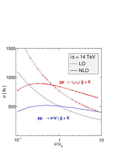
Figure 2: Scale dependence of the total LHC cross section at LO and NLO for $pp\to e^{+}e^{-}\gamma jj+X$ and $pp\to\nu_{e}\bar{\nu}_{e}\gamma jj+X$ production around the central scale $\mu_{0}$ defined in Eq. 4. The cuts used are described in the text.

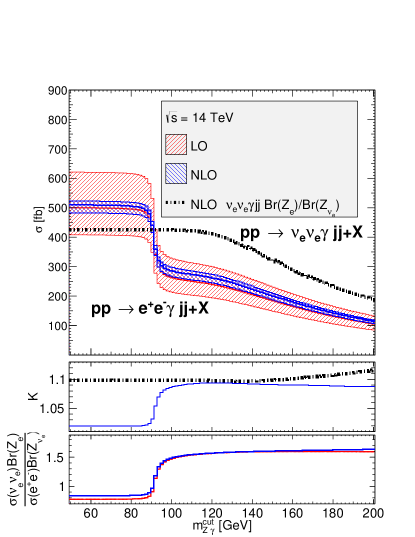
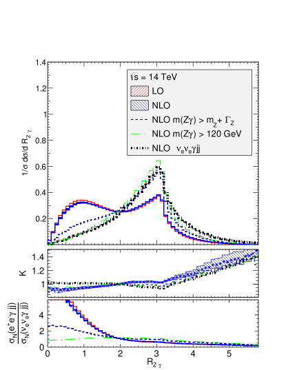
Figure 3: Left: Cross section for different values of the reconstructed $Z\gamma$ invariant mass cut. The neutrino curve is multiplied by the ratio of the charge-lepton versus neutrino branching ratios. The middle panel shows the K-factor and the lower the ratios of the modified neutrino cross section versus the LO and NLO electron cross sections. Right: Normalized differential distributions of the rapidity-azimuthal angle separation $R_{Z\gamma}$ for different values of the $m_{Z\gamma}^{\,\mathrm{cut}}$ cut. The middle and lower panels show the differential K-factor plots and the ratios of the normalized electron versus neutrino pair production channels.

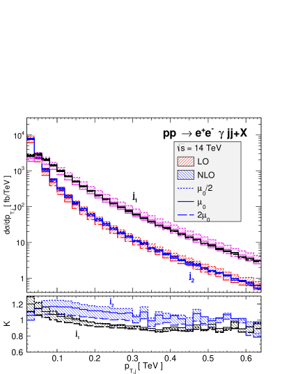
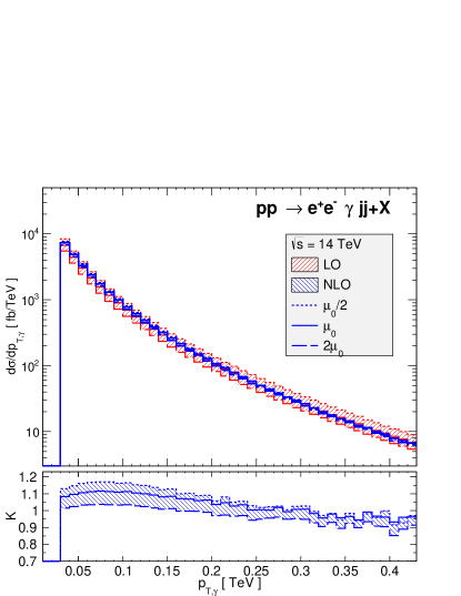
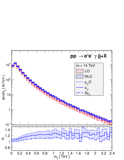
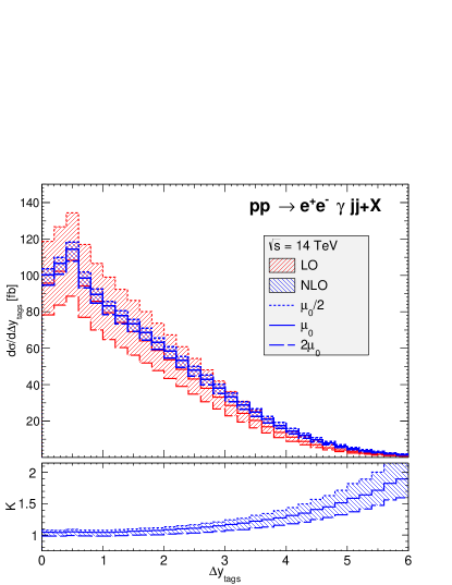
Figure 4: Differential distributions for the transverse momentum of the tagging jets (top left) and the photon (top right). On the bottom, the invariant mass (left) and rapidity separation (right) of the two tagging jets are displayed. The bands show the scale variations around the central scale, $\mu_{0}/2\leq\mu_{F}=\mu_{R}\leq 2\mu_{0}$. In the small panels, the differential K-factors are plotted. The bands reflect the NLO scale variations with respect to $\sigma_{\text{LO}}(\mu_{0})$. The inclusive cuts described in the text are used together with the cut on the invariant mass of the $Z\gamma$ system, $m_{Z\gamma}^{\text{cut}}=120\,\mathrm{GeV}$, which eliminates the final radiative emission off the charged leptons.

Other input parameters are chosen as $M_{Z}=91.1876\,\mathrm{GeV}$, $M_{W}=80.385\,\mathrm{GeV}$ and $G_{F}=1.16637\times 10^{-5}\,\mathrm{GeV}^{-2}$. The electromagnetic coupling constant and the weak-mixing angle are calculated via tree level relations. All fermions are taken to be massless, except the top quark with $m_{t}=173.1\,\mathrm{GeV}$. The width of the $Z$ is fixed at $\Gamma_{Z}=2.508905\,\mathrm{GeV}$. The strong coupling constant is renormalized using the $\overline{\,\mathrm{MS}}$ scheme. The top-quark contribution is decoupled from the running, but is explicitly included in the one-loop amplitude. As a central factorization and renormalization scale, we use the sum of the transverse energy $E_{T}=(p_{T}^{2}+p^{2})^{1/2}$ of the two tagging jets and of the reconstructed $Z\gamma$ system,

$$\mu_{F}=\mu_{R}=\mu_{0}=\frac{1}{2}\left[E_{T}(jj)+E_{T}(VV)\right].$$ (4)

The first term interpolates between $m_{jj}$ and $\sum p_{T,jets}$ for large and small $\Delta y_{jj}$ values, characterizing the dynamics of these processes appropriately.

In the following, we present results for the first generation of leptons. Taking into account both the electron and the muon yields an extra factor of two. Summing over three generations of neutrinos gives a factor of three.

To evaluate the scale uncertainties associated to a fixed order calculation, we plot in Fig. 2 the cross section for the “$Z_{\nu}\gamma jj$ ” and “$Z_{l}\gamma jj$ ” channels varying the central scale in the range $\mu\in(10^{-1},10)\mu_{0}$ simultaneously for the factorization and the renormalization scale, which are set equal for simplicity. At the central scale, we obtain $\sigma_{\,\mathrm{\text{LO}}}=500.82(3)^{+24\%}_{-18\%}\,\mathrm{fb}$ and $\sigma_{\,\mathrm{\text{NLO}}}=510.6(1)^{+2.6\%}_{-5.3\%}\,\mathrm{fb}$ for the $e^{+}e^{-}\gamma jj$ channel and $\sigma_{\,\mathrm{\text{LO}}}=765.58(3)^{+26\%}_{-19\%}\,\mathrm{fb}$ and $\sigma_{\,\mathrm{\text{NLO}}}=840.8(3)^{+5.3\%}_{-7\%}\,\mathrm{fb}$ for the $\bar{\nu}_{e}\nu_{e}\gamma jj$ one. The upper and lower numbers correspond to the scale uncertainties in percentage for variations of a factor 2 around the central scale and the number in brackets is the Monte-Carlo statistical error. At the central scale, we observed very mild K-factors, defined as the ratio of the NLO over LO predictions of the order of $1.01$ and $1.1$ for the “$Z_{l}\gamma jj$” and “$Z_{\nu}\gamma jj$” channels, respectively.

Next we investigate the radiative photon emission off the charged leptons in the “$Z_{l}\gamma jj$ ” channel (see the middle Feynman diagrams of Fig. 1). These radiative decays present in both the EW and QCD induced processes reduce the sensitivity to anomalous-coupling searches and therefore it is desirable to suppress them. This contribution dominates in the phase-space region where the reconstructed invariant mass of the $Z\gamma$ system is close to the $Z$ mass. Thus, imposing a cut on $M_{Z\gamma}$ around the $Z$ mass should remove this contribution. The optimum value of the cut is a priori uncertain. We therefore use the “$Z_{\nu}\gamma jj$ ” channel, where radiative decays are absent, to determine it.

In the left panel of Fig. 3, as functions of the $m_{Z\gamma}$ cut, we plot the integrated NLO cross sections for the “$Z_{l}\gamma jj$” and “$Z_{\nu}\gamma jj$” channels, the latter being multiplied by the ratio of the charge-lepton versus neutrino branching ratios of the $Z$, $Br(Z\to e^{+}e^{-})/Br(Z\to\bar{\nu}_{e}{\nu}_{e})=0.506$. The LO cross section is also shown for the “$Z_{l}\gamma jj$” channel. In the bottom panel, the ratios of the modified neutrino cross sections to the LO and NLO electron cross sections are plotted. They do not converge to one in the tails due to the different cuts applied for the charged leptons and the neutrinos. As expected, for the charged-lepton case, one observes that the cross section sharply decreases when the cut value is greater than the $Z$ mass. In the middle panel, the K-factors are plotted. We observe that $m_{Z\gamma}^{\text{cut}}=120\,\mathrm{GeV}$ is a good value since the K-factor exhibits a plateau and the slope of the cross section curves are approximately equal for both processes beyond this value (see bottom panel). This is confirmed in the right panel of Fig. 3, where the normalized differential distributions of the reconstructed rapidity-azimuthal angle separation of the $Z\gamma$ system are plotted for the two channels. One observes that the cut $m_{Z\gamma}>m_{Z}+\Gamma_{Z}$ reduces considerably the effect of the radiative decay in the charged-lepton channel, but some remnant is still clearly visible by comparing to the neutrino channel. Increasing the cut value to $120\,\mathrm{GeV}$ makes the NLO distribution of the “$Z_{l}\gamma jj$” channel very similar to the corresponding “$Z_{\nu}\gamma jj$” one. This is better seen in the bottom panel, where the ratios of the normalized differential distributions between the two channels are plotted. The ratio of the $m_{Z\gamma}^{\text{cut}}=120\,\mathrm{GeV}$ curve versus the “$Z_{\nu}\gamma jj$” distribution is rather flat and close to one till $R_{Z\gamma}$ reaches values of around 3 and then decreases. This difference is probably again due to the different cuts applied between the charged leptons and the neutrinos.

In the following, we impose an additional cut $m_{Z\gamma}>120\,\mathrm{GeV}$ and plot some relevant differential distributions for the two tagging jets and the photon at LO and NLO in the large panels of Fig. 4. The tagging jets are defined as the two jets with highest transverse momenta and are ordered by hardness. The bands show the scale uncertainty in the range $\mu_{0}/2\leq\mu_{F}=\mu_{R}\leq 2\mu_{0}$. The small panels always show the differential K-factors where the bands represents the scale variations of the NLO result, with respect to $\sigma_{\text{LO}}(\mu_{0})$. In the top row, the differential distributions of the transverse momentum of the two tagging jets (left) and the photon (right) are plotted. The bottom row displays the invariant mass (left) and the rapidity difference (right) of the two tagging jets. As expected, the scale uncertainty decreases considerably at NLO. Note that the rapidity-separation distribution receives large NLO QCD corrections in the region selected for vector boson fusion scattering, $\Delta y_{\text{tags}}>3$. In general, the size of the K-factors range from $0.8$ to $1.9$, showing that NLO predictions are necessary for accurate measurements.

IV Conclusions

In this article, we have presented first results at NLO in QCD for the $pp\to l^{+}l^{-}\gamma jj+X$ and $pp\to\bar{\nu}_{l}\nu_{l}\gamma jj+X$ processes. With this result, all the QCD-induced $VVjj$ production processes are known at NLO QCD.

By comparing against the neutrino production process, we have been able to efficiently remove the contribution of radiative photon emission off the charged leptons, which diminishes the sensitivity of EW-induced processes to anomalous couplings. As expected, the scale uncertainty is significantly reduced at NLO, which is visible both at the total and differential cross section level. The size of the NLO QCD corrections are phase space dependent ranging from $-20\%$ to $+90\%$, and are particularly large in the region where the vector-boson scattering signal is enhanced. NLO corrections are therefore needed for reliable predictions.

V Acknowledgments

FC acknowledges financial support by the IEF-Marie Curie program (PIEF-GA-2011-298960) and partial funding by the LHCPhenonet (PITN-GA-2010-264564) and by the MINECO (FPA2011-23596). MK is funded by the graduate program GRK 1694: “Elementary particle physics at highest energy and precision”. LDN and DZ are supported in part by the Deutsche Forschungsgemeinschaft via the Sonderforschungsbereich/Transregio SFB/TR-9 “Computational Particle Physics”

*

Appendix A Results at one phase-space point

In the following, we present results at one phase-space point for the virtual amplitudes to facilitate comparison with future calculations. We chose the same phase-space momentum configuration as Ref. Campanario:2014dpa , Table 1, and give results for the process $j_{1}j_{2}\to j_{3}j_{4}e^{+}e^{-}\gamma$ at the squared-amplitude level, averaging over the initial-state helicities and colors.

Table 1: Momenta (in $\,\mathrm{GeV}$) at a random phase-space point for $j_{1}j_{2}\to j_{3}j_{4}e^{+}e^{-}\gamma$ subprocesses.

	$E$		$p_{x}$		$p_{y}$		$p_{z}$
$j_{1}$	32.	0772251055223	0.	0	0.	0	32.	0772251055223
$j_{2}$	2801.	69305619768	0.	0	0.	0	-2801.	69305619768
$j_{3}$	226.	525314156010	-10.	2177083492279	-1.	251308382450315$\times 10^{-15}$	-226.	294755550298
$j_{4}$	327.	281588297290	-6.	48554750244653	-10.	1061447270513	-327.	061219882068
$e^{+}$	646.	824307052136	36.	0746355875450	-26.	0379256562231	-645.	292438579767
$e^{-}$	1598.	85193997112	-2.	88431497177613	24.	4490976584709	-1598.	66239347157
$\gamma$	34.	2871318266438	-16.	4870647640944	11.	6949727248035	27.	6949763915464

Table 2: QCD interference amplitudes $2\text{Re}(\mathcal{A}_{\text{NLO}}\mathcal{A}^{*}_{\text{LO}})$ for $j_{1}j_{2}\to j_{3}j_{4}e^{+}e^{-}\gamma$ subprocesses.

	$1/\epsilon^{2}$		$1/\epsilon$		finite
			$uu\to uu$
I operator	2.	1930022552$\times 10^{-2}$	3.	6933147142$\times 10^{-2}$	7.	311094745$\times 10^{-2}$
loop	-2.	19300225$\times 10^{-2}$	-3.	6933147$\times 10^{-2}$	0.	14424709
I+loop	3.	6$\times 10^{-14}$	5.	9$\times 10^{-13}$	0.	2173580
			$uc\to uc$
I operator	3.	1917977819$\times 10^{-2}$	5.	1904760292$\times 10^{-2}$	0.	1098476201
loop	-3.	19179778$\times 10^{-2}$	-5.	19047603$\times 10^{-2}$	0.	196364213
I+loop	9.	5$\times 10^{-14}$	1.	1$\times 10^{-12}$	0.	30621183
			$ud\to ud$
I operator	5.	9210009570$\times 10^{-2}$	9.	6286844080$\times 10^{-2}$	0.	2037747651
loop	-5.	92100095$\times 10^{-2}$	-9.	628684$\times 10^{-2}$	0.	53005178
I+loop	3.	0$\times 10^{-13}$	1.	4$\times 10^{-9}$	0.	7338265
			$dd\to dd$
I operator	6.	8465222944$\times 10^{-3}$	1.	1487721719$\times 10^{-2}$	2.	246881141$\times 10^{-2}$
loop	-6.	84652229$\times 10^{-3}$	-1.	14877217$\times 10^{-2}$	4.	789599960$\times 10^{-2}$
I+loop	2.	5$\times 10^{-14}$	2.	5$\times 10^{-13}$	7.	03648110$\times 10^{-2}$
			$ds\to ds$
I operator	1.	04197858244$\times 10^{-2}$	1.	6944572384$\times 10^{-2}$	3.	586031267$\times 10^{-2}$
loop	-1.	041978582$\times 10^{-2}$	-1.	69445724$\times 10^{-2}$	6.	930377376$\times 10^{-2}$
I+loop	5.	6$\times 10^{-14}$	4.	9$\times 10^{-13}$	0.	105164086
			$gg\to\bar{u}u$
I operator	4.	2224900184$\times 10^{-4}$	2.	5147277683$\times 10^{-5}$	5.	73018157$\times 10^{-4}$
loop	-4.	2224900$\times 10^{-4}$	-2.	51472$\times 10^{-5}$	1.	24085333$\times 10^{-3}$
I+loop	2.	6$\times 10^{-14}$	2.	4$\times 10^{-13}$	1.	81387148$\times 10^{-3}$
			$gg\to\bar{d}d$
I operator	1.	13509295313$\times 10^{-4}$	6.	3611573393$\times 10^{-6}$	1.	56909560$\times 10^{-4}$
loop	-1.	135092953$\times 10^{-4}$	-6.	36116$\times 10^{-6}$	3.	27276628$\times 10^{-4}$
I+loop	5.	4$\times 10^{-16}$	2.	4$\times 10^{-14}$	4.	8418618$\times 10^{-4}$

We include all UV counterterms and all closed-quark loops with gluons attached to it. Diagrams including a closed-quark loop with the $Z/\gamma^{*}$ directly attached to it are excluded. The top quark is decoupled from the running of $\alpha_{s}$. However, its contribution is explicitly included in the one-loop amplitudes. Here we use $\alpha=\alpha_{s}=1$ for simplicity. With this set up and measuring energies in $\,\mathrm{GeV}$, we get at tree level,

$$\overline{|\mathcal{A}_{\text{LO}}^{uu\rightarrow uu}|}^{2} =2.583569915405990\times 10^{-2},$$

$$\overline{|\mathcal{A}_{\text{LO}}^{uc\rightarrow uc}|}^{2} =3.760248173799574\times 10^{-2},$$

$$\overline{|\mathcal{A}_{\text{LO}}^{ud\rightarrow ud}|}^{2} =6.975514915738625\times 10^{-2},$$

$$\overline{|\mathcal{A}_{\text{LO}}^{dd\rightarrow dd}|}^{2} =8.065869053590906\times 10^{-3},$$

$$\overline{|\mathcal{A}_{\text{LO}}^{ds\rightarrow ds}|}^{2} =1.227552097429276\times 10^{-2},$$

$$\overline{|\mathcal{A}_{\text{LO}}^{gg\rightarrow\bar{u}u}|}^{2} =3.061233143517198\times 10^{-4},$$

$$\overline{|\mathcal{A}_{\text{LO}}^{gg\rightarrow\bar{d}d}|}^{2} =8.229230037027499\times 10^{-5}.$$ (5)

For the one-loop integrals, we use the convention

$$T_{0}=\frac{\mu_{R}^{2\epsilon}\Gamma(1-\epsilon)}{i\pi^{2-\epsilon}}\int d^{D}q\frac{1}{(q^{2}-m_{1}^{2}+i0)\cdots},$$ (6)

with $D=4-2\epsilon$. Additionally, the conventional dimensional regularization method 'tHooft:1972fi with $\mu_{R}=M_{Z}$ is used. With this, the interference amplitudes $2\text{Re}(\mathcal{A}_{\text{NLO}}\mathcal{A}^{*}_{\text{LO}})$, for the one-loop corrections and the I-operator contribution as defined in Ref. Catani:1996vz , are given in Table 2.

Switching from the conventional dimensional regularization to dimensional reduction method induces a finite shift, which can be calculated noting that the sum $|\mathcal{A}_{\text{LO}}|^{2}+2\text{Re}(\mathcal{A}_{\text{NLO}}\mathcal{A}^{*}_{\text{LO}})$ should be constant Catani:1996pk . The shift on the Born amplitude squared comes from the change in the strong coupling constant, see e.g. Ref. Kunszt:1993sd ,

$$\alpha_{s}^{\overline{DR}}=\alpha_{s}^{\overline{MS}}\left(1+\frac{\alpha_{s}}{4\pi}\right).$$ (7)

Finally, using the rule given in Ref. Catani:1996vz , the shift on the I-operator contribution can be calculated.

References

- (1) J. Bernabeu, F. Campanario, and J. Parra, In preparation .
- (2) G. Bozzi, F. Campanario, V. Hankele, and D. Zeppenfeld, Phys.Rev. D81, 094030 (2010), arXiv:0911.0438.
- (3) G. Bozzi, F. Campanario, M. Rauch, H. Rzehak, and D. Zeppenfeld, Phys.Lett. B696, 380 (2011), arXiv:1011.2206.
- (4) K. Arnold et al., Comput.Phys.Commun. 180, 1661 (2009), arXiv:0811.4559.
- (5) K. Arnold et al., (2011), 1107.4038.
- (6) J. Baglio et al., (2014), 1404.3940.
- (7) F. Campanario, M. Kerner, L. D. Ninh, and D. Zeppenfeld, Phys.Rev. D89, 054009 (2014), 1311.6738.
- (8) J. Alwall et al., (2014), 1405.0301.
- (9) T. Melia, K. Melnikov, R. Rontsch, and G. Zanderighi, JHEP 1012, 053 (2010), arXiv:1007.5313.
- (10) T. Melia, K. Melnikov, R. Rontsch, and G. Zanderighi, Phys.Rev. D83, 114043 (2011), arXiv:1104.2327.
- (11) N. Greiner et al., Phys.Lett. B713, 277 (2012), arXiv:1202.6004.
- (12) A. Denner, L. Hosekova, and S. Kallweit, Phys.Rev. D86, 114014 (2012), arXiv:1209.2389.
- (13) F. Campanario, M. Kerner, L. D. Ninh, and D. Zeppenfeld, Phys. Rev. Lett. 111, 052003 (2013), arXiv:1305.1623.
- (14) T. Gehrmann, N. Greiner, and G. Heinrich, Phys.Rev.Lett. 111, 222002 (2013), 1308.3660.
- (15) S. Badger, A. Guffanti, and V. Yundin, JHEP 1403, 122 (2014), 1312.5927.
- (16) F. Campanario, M. Kerner, L. D. Ninh, and D. Zeppenfeld, (2014), 1402.0505.
- (17) Z. Bern et al., (2014), 1402.4127.
- (18) F. Campanario, M. Kerner, L. D. Ninh, and D. Zeppenfeld, (2014), 1405.3972.
- (19) S. Frixione, Phys.Lett. B429, 369 (1998), hep-ph/9801442.
- (20) K. Hagiwara and D. Zeppenfeld, Nucl.Phys. B313, 560 (1989).
- (21) F. Campanario, JHEP 1110, 070 (2011), arXiv:1105.0920.
- (22) T. Gleisberg et al., JHEP 0902, 007 (2009), arXiv:0811.4622.
- (23) T. Gleisberg and S. Hoeche, JHEP 0812, 039 (2008), arXiv:0808.3674.
- (24) A. Martin, W. Stirling, R. Thorne, and G. Watt, Eur.Phys.J. C63, 189 (2009), arXiv:0901.0002.
- (25) G. ’t Hooft and M. Veltman, Nucl.Phys. B44, 189 (1972).
- (26) S. Catani and M. Seymour, Nucl.Phys. B485, 291 (1997), hep-ph/9605323.
- (27) S. Catani, M. Seymour, and Z. Trocsanyi, Phys.Rev. D55, 6819 (1997), hep-ph/9610553.
- (28) Z. Kunszt, A. Signer, and Z. Trocsanyi, Nucl.Phys. B411, 397 (1994), hep-ph/9305239.