The circumgalactic medium of high redshift galaxies
Abstract
We study the properties of the circumgalactic medium (CGM) of high- galaxies in the metal enrichment simulations presented in Pallottini et al. (2014). At , we find that the simulated CGM gas density profiles are self-similar, once scaled with the virial radius of the parent dark matter halo. We also find a simple analytical expression relating the neutral hydrogen equivalent width () of CGM absorbers as a function of the line of sight impact parameter (). We test our predictions against mock spectra extracted from the simulations, and show that the model reproduces the profile extracted from the synthetic spectra analysis. When compared with available data, our CGM model nicely predicts the observed in galaxies, and supports the idea that the CGM profile does not evolve with redshift.
keywords:
cosmology: simulations – circumgalactic medium.1 Introduction
The circumgalactic medium (CGM) is the extended interface between the interstellar medium (ISM) of a galaxy and the surrounding intergalactic medium (IGM). This component plays a key role in galactic evolution as it represents a mass reservoir and a repository of the mechanical and radiative energy produced by stars. Due to its low density, the CGM can be almost uniquely traced by absorption line experiments towards background sources, typically quasars. The intervening CGM associated with a foreground galaxy then leaves a characteristic spectral feature. Provided that a sufficiently large sample of galaxies are available it is then possible to statistically determine the Equivalent Width () of a given absorption line as a function of the line of sight (l.o.s.) impact parameter ().
The CGM has been probed so far up to using absorption lines of both H (e.g. Rudie et al., 2012, 2013; Pieri et al., 2013) and heavy elements (e.g. Steidel et al., 2010; Churchill et al., 2013; Nielsen et al., 2013; Borthakur et al., 2013; Jia Liang & Chen, 2014). These observations show that the CGM extends up to , where is the virial radius of the parent dark matter (DM) halo. An anticorrelation between and is observed; moreover, the profiles appear to be self-similar once scaled with . Finally Chen (2012) suggested that CGM absorption profiles show no signs of evolution from to .
In the framework of a CDM111Hereafter we assume a CDM cosmology with , , , , , , (Larson et al., 2011). cosmological model, the CGM properties can be derived from numerical simulations simultaneously accounting for both large scale ( Mpc) structure and small scale ( kpc) galactic feedback. While such a huge dynamical range makes a truly self-consistent simulation impossible, these difficulties can be overcome by following the unresolved physical scales with subgrid models.
Along these lines, some numerical studies have focused on testing CGM metal enrichment models (e.g. Shen et al., 2013; Barai et al., 2013; Crain et al., 2013); others have investigated the imprint of the last phases of reionization on the IGM/CGM (e.g. Finlator et al., 2013; Keating et al., 2014) or the ISM/CGM overdensity-metallicity (-) relation as a function of redshift (Pallottini et al., 2014, hereafter P14). Surprisingly, little attention has been devoted so far to understand the physics beneath the observed CGM profile self-similarity and redshift independence.
In this Letter we show that the previously found - relation naturally arises from self-similar nature of the CGM density/metallicity profiles. We use this result to derive an analytical expression for which we then test against synthetic spectra extracted from the simulations and available observational data.
2 Numerical simulations
We adopt the simulations described in P14 which were obtained by using a customized version of the Adaptive Mesh Refinement code ramses (Teyssier, 2002). Starting from cosmological initial conditions generated at , we evolve a Mpc volume until . The DM mass resolution is , and the adaptive baryon spatial resolution ranges from kpc to kpc.
We include subgrid prescriptions for star formation, accounting for supernova (thermal) feedback and implementing metal-dependent stellar yields and return fractions. Our simulation reproduces the observed cosmic star formation rate (Bouwens et al., 2012) and stellar mass densities (González et al., 2011) for .
We define a galactic environment as a connected patch of enriched gas with metallicity exceeding a chosen threshold, i.e. . Within such regions, following a common classification, we identify three different phases according to their gas overdensity: IGM (), CGM (), and ISM ().
In P14 we have shown how to construct a complete catalogue of galactic environments at a given redshift. To each galactic environment we associate the group of DM halos, of total mass , inside its boundary. We denote as “central halo” the most massive halo in each group and “satellites” the remaining ones. Since the central halo dominates the local dynamics, we use its mass () to compute the virial radius of the structure ().
2.1 Self-similar and profiles
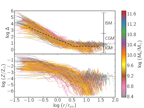
We focus our attention at , the lowest redshift reached by the simulation. At this epoch a - relation for the gas is already in place. Fig. 1 shows the spherically-averaged radial profiles of the overdensity (upper panel) and metallicity (lower panel), as a function of , for various () simulated galactic environments characterized by .
The overdensity trend is very similar for all galactic environments. In particular, the ISM is located at , the CGM spans the radial range and the IGM extends beyond . Hence, the adopted density definition for different gas phases is equivalent to a distance classification222Therefore we will use interchangeably overdensity and distance definitions for the three phases., similarly to the proposal by Shull (2014).
Generally, one might expect that the shape of the relation depends somewhat on feedback prescriptions (Oppenheimer et al., 2012). However, we note that feedback has been accurately calibrated in P14 to reproduce globally averaged galactic properties.
The gas density profile can then be written in terms of the self-similar variable as a piecewise power-law of index :
| (1) |
where is the gas density evaluated at the virial radius, is the Heaviside function and denotes the location where the density approaches a constant value typical of the IGM in the proximity of galactic systems. The best fit values for the parameters are: , and . From the fit, we also find the relation . In the upper panel of Fig. 1, is shown by the black dashed line.
The metallicity (Fig. 1, lower panel) is essentially flat in the ISM and rapidly declines in the CGM; this result is independent from the selected environment. The trend is however not universal in the IGM, as expected from the results of P14, where we showed that is only weakly correlated with in the IGM. Environments associated with massive DM halos () show an enriched () IGM up to . Instead, halos with , which contain small galaxy groups or even isolated galaxies, only manage to pollute the IGM within . This trend is discussed in detail in Fig. 13 of P14.
Finally, galaxies hosted in halos with masses lower than only show up as satellites (P14). Their effect is perceivable in Fig. 1 as a local perturbation to the global and trends at . The satellite positions resulting from our simulation are in broad agreement with the outcome of the numerical simulation by Khandai et al. (2014), who find a flat satellite distribution at for (see their Fig. 10).
2.2 Modeling H absorption
From the fit to the simulated density profile, , we build a simple analytical model that describes the H absorption properties (NHI and EWHI) of the CGM/IGM.
The H column density along a l.o.s. is defined as , where is the total hydrogen density, and is the H fraction. Assuming spherical symmetry, we express through the following relation:
| (2) |
where is given in eq. 1, is the impact parameter, is hydrogen mass, , is the Hubble constant and is the velocity window sampled by observations. Assuming local photoionization equilibrium (e.g. Dayal et al., 2008), the H fraction can be written as , where , is the recombination rate and is the UV background photoionization rate. Consistent with P14 simulations, we use the UV intensity from Haardt & Madau (2012).
The H Ly equivalent width can be expressed as follows:
| (3) |
where is the speed of light, is the frequency of the Ly transition, is the Voigt profile (e.g. Meiksin, 2009), is the thermal Doppler broadening and , where is the oscillator strength, and are the electron mass and charge, respectively. By combining eq.s 1-3, we obtain the trend of with , for different values of and .
The dependence on , entering through the density dependence on , results in a stretching/compression of the density profile. The temperature , entering in the expressions for and , regulates both H at and the slope of the profile for . For increasing (decreasing) values, H is shifted downward (upward) while the slope becomes steeper (shallower). It is worth noticing that we are assuming a single temperature value both for the IGM and CGM. Moreover, we are neglecting turbulence, which may affect the Doppler broadening of CGM absorbers (e.g. Iapichino et al., 2013). Therefore, must be regarded as an “effective temperature”; to make it clear we will use to indicate this quantity.
3 Testing the H absorption model
We are now ready to test our model both against simulated QSO absorption spectra and real data.
3.1 Synthetic H absorption spectra
We compute mock QSO absorption spectra along several l.o.s. drawn through the simulated box. The technique adopted to compute the H optical depth is detailed in Gallerani et al. (2006). In order to reproduce the mean transmitted flux observed at (, Becker et al. 2013) the intensity of the UV ionizing background (Haardt & Madau, 2012) assumed in the simulation is rescaled upwards by a factor 6.6, resulting into a photoionization rate . We also include observational artifacts in our simulated spectra, following Rudie et al. (2013), a work based on HIRES spectra. We smooth the synthetic spectra to a resolution , add to each pixel a Gaussian random deviate, yielding a signal-to-noise ratio , and we finally rebin the simulated transmitted flux in channels of width 0.4 A.
Among the l.o.s. extracted from the simulations, we select the ones passing through a specific galactic environment, defined by its central halo and its corresponding . The sample of l.o.s. considered encompasses a wide range of impact parameters, namely - .
3.2 Largest gap statistics
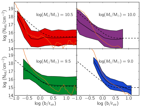
Along each l.o.s, we identify the CGM absorption feature with the largest spectral gap333Spectral gaps are defined as contiguous regions of the spectrum having an optical depth over rest-frame intervals A (Croft, 1998). found in the corresponding synthetic spectrum (Gallerani et al., 2008a, b). In order to check that largest gaps correctly identify CGM absorption features, we compute the along their corresponding l.o.s. paths, for different values, and for a set of galactic environments characterized by and , that correspond at to and , respectively.
The results from a sample of 3000 l.o.s. are shown in Fig. 2. Superimposed to the profiles obtained from the synthetic spectra analysis, are the average values inferred from the P14 simulations444 For each l.o.s., , where the integration limits correspond to the borders of the environment, which in turn depend on . Changing the metallicity threshold marginally affects the results: using yields a variation of for the inferred column density. The orange lines are obtained by averaging over l.o.s.. and the column density resulting from the analytical model (eq. 2) calculated for . Fig. 2 shows that the largest gap statistics properly identifies CGM absorption features in H absorption spectra.
This technique is particularly promising for studying the CGM absorption properties for high- () quasar spectra. At these redshifts, the maximum observed transmitted flux drops below 50% in the Ly forest (Songaila, 2004). The resulting large uncertainties in the continuum determination may therefore hamper a proper Voigt profile analysis.
3.3 Comparison with simulations
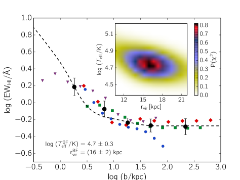
As a next step, we compute the of the absorption features identified through the largest gap statistics as a function of the parameters, for the galactic environments presented in Fig. 2. The results are shown in the left panel of Fig. 3 through red diamonds, purple downwards triangles, green squares, and blue circles for and , respectively. In the same figure, black circles and corresponding error bars represent mean and r.m.s. values obtained by averaging the profiles of the 4 different galactic environments into bins of width such that . As expected (see eq. 3), the profiles follow the trend (Fig. 2), namely decreases with .
Finally, we fit the averaged profile resulting from the synthetic spectra analysis through our analytical model, finding the following best fit parameters: and kpc. The inferred value agrees with typical values of the CGM/IGM temperature (P14) and is consistent with the average virial radius of the galactic environments considered, namely kpc. This result represents a solid consistency check of our model which allows us to repeat the same experiment on real data.
3.4 Comparison with observations
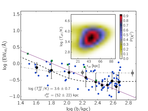
In the right panel of Fig. 3, we compare our model with observations. Blue circles are the derived at by Jia Liang & Chen (2014); black circles and corresponding error bars represent mean and r.m.s. values obtained by averaging the same observational data into bins kpc large.
For this comparison the model is calculated with , i.e. the value at given by Haardt & Madau (2012). By fitting555Supported by the lack of evolution of CGM profiles from to (Chen, 2012), we assume to be redshift independent in eq. 1. observations with our analytical model we find and kpc. provides only an indicative value for the average temperature of the CMG/IGM. Although is consistent within 1.2 with the mean virial radius kpc quoted by Jia Liang & Chen (2014), we note that our model favors smaller values.
The dashed black line in the right panel of Fig. 3 represents our best fit model, while the violet solid line shows the model from Chen et al. (1998, 2001, hereafter C-model). Both the C-model and our best fit are in agreement with Jia Liang & Chen (2014) observations up to , i.e. in the CGM range (). On the other hand, for , the C-model declines more steeply than data, while our best fit model properly reproduces the observed flat trend.
The gray circles linked by the dashed dotted line show the EW profile obtained from synthetic spectra, once rescaled to the of the model which reproduces observations. The good agreement between the synthetic and observed EWHI(b) profiles, both shows that our modelling of the CGM reproduces observations, and favors the scenario suggested by Chen (2012) of a redshift independent CGM profile. As a further support to this idea we also show (green squares) CGM observations at by Steidel et al. (2010), which are perfectly consistent both with observations and with the EW profile obtained from synthetic spectra.
4 Projected - relation
Inspired by the - relation found in the ISM/CGM, we investigate whether the mean metallicity along a simulated l.o.s. correlates with the distribution of our galactic environments. We compute through the following equation: .
In Fig. 4, we plot the probability distribution function (PDF) of and for a simulated environment characterized by . Consistently with observations of the CGM in the proximity of halos (i.e. Jia Liang & Chen, 2014), we find an upper limit of in the simulated CGM.
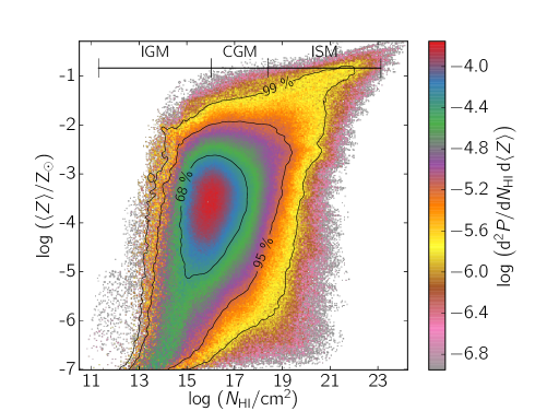
Fig. 4 shows that tightly correlates with only in the ISM, which displays both high column density () and high mean metallicity () values. However, for the CGM/IGM, the underlying tight - correlation is somewhat blurred, once projected into the and variables, which present larger dispersions. This result implies that H absorption studies do not allow to precisely constrain the CGM metallicity, as a consequence of a strong – degeneracy.
Such a degeneracy can only be broken by adding metal absorption line information. In this case, proximity effect of ionizing sources may turn out to be crucial in determining the different ionization levels of metal atoms. We defer to a future work a proper inclusion of these radiative transfer effects in our simulation. This will allow us to correctly interpret high- CGM/IGM metal absorption line observations (e.g. D’Odorico et al., 2013; Gonzalo Díaz et al., 2014).
5 Conclusions
We have used a cosmological metal enrichment simulation (Pallottini et al., 2014) to study the CGM/IGM properties of high- galaxies, by analyzing the H absorption profiles of the simulated galactic environments. The main results can be summarized as follows:
- 1.
-
2.
Using simulations, we have produced mock H absorption spectra which are then analyzed using the largest gap statistics to identify CGM absorption features. As a consistency check of the model, we have verified that it can reproduce the analogous profile deduced from the synthetic spectra.
- 3.
-
4.
We have investigated the relation between the mean metallicity along a simulated l.o.s. and the distribution of galactic environments. Consistently with metal absorption line observations of Jia Liang & Chen (2014), we find in the CGM; however, the strong – degeneracy does not allow to constrain the CGM metallicity through H absorption studies alone, and metal absorption line information is required to this goal.
Acknowledgments
We are grateful to E. Komatsu and L. Vallini for fruitful discussions.
References
- Barai et al. (2013) Barai P. et al., 2013, MNRAS, 430, 3213
- Borthakur et al. (2013) Borthakur S., Heckman T., Strickland D., Wild V., Schiminovich D., 2013, ApJ, 768, 18
- Bouwens et al. (2012) Bouwens R. J. et al., 2012, ApJ, 754, 83
- Chen (2012) Chen H.-W., 2012, MNRAS, 427, 1238
- Chen et al. (1998) Chen H.-W., Lanzetta K. M., Webb J. K., Barcons X., 1998, ApJ, 498, 77
- Chen et al. (2001) Chen H.-W., Lanzetta K. M., Webb J. K., Barcons X., 2001, ApJ, 559, 654
- Churchill et al. (2013) Churchill C. W., Trujillo-Gomez S., Nielsen N. M., Kacprzak G. G., 2013, ApJ, 779, 87
- Crain et al. (2013) Crain R. A., McCarthy I. G., Schaye J., Theuns T., Frenk C. S., 2013, MNRAS, 432, 3005
- Croft (1998) Croft R. A. C., 1998, in Eighteenth Texas Symposium on Relativistic Astrophysics, Olinto A. V., Frieman J. A., Schramm D. N., eds., p. 664
- Dayal et al. (2008) Dayal P., Ferrara A., Gallerani S., 2008, MNRAS, 389, 1683
- D’Odorico et al. (2013) D’Odorico V. et al., 2013, MNRAS, 435, 1198
- Finlator et al. (2013) Finlator K., Muñoz J. A., Oppenheimer B. D., Oh S. P., Özel F., Davé R., 2013, MNRAS, 436, 1818
- Gallerani et al. (2006) Gallerani S., Choudhury T. R., Ferrara A., 2006, MNRAS, 370, 1401
- Gallerani et al. (2008a) Gallerani S., Ferrara A., Fan X., Choudhury T. R., 2008a, MNRAS, 386, 359
- Gallerani et al. (2008b) Gallerani S., Salvaterra R., Ferrara A., Choudhury T. R., 2008b, MNRAS, 388, L84
- González et al. (2011) González V., Labbé I., Bouwens R. J., Illingworth G., Franx M., Kriek M., 2011, ApJL, 735, L34
- Gonzalo Díaz et al. (2014) Gonzalo Díaz C., Koyama Y., Ryan-Weber E. V., Cooke J., Ouchi M., Shimasaku K., Nakata F., 2014, ArXiv:1404.7656
- Haardt & Madau (2012) Haardt F., Madau P., 2012, ApJ, 746, 125
- Iapichino et al. (2013) Iapichino L., Viel M., Borgani S., 2013, MNRAS, 432, 2529
- Jia Liang & Chen (2014) Jia Liang C., Chen H.-W., 2014, ArXiv 1402.3602
- Keating et al. (2014) Keating L. C., Haehnelt M. G., Becker G. D., Bolton J. S., 2014, MNRAS, 438, 1820
- Khandai et al. (2014) Khandai N., Di Matteo T., Croft R., Wilkins S. M., Feng Y., Tucker E., DeGraf C., Liu M.-S., 2014, ArXiv 1402.0888
- Larson et al. (2011) Larson D. et al., 2011, ApJS, 192, 16
- Meiksin (2009) Meiksin A. A., 2009, Reviews of Modern Physics, 81, 1405
- Nielsen et al. (2013) Nielsen N. M., Churchill C. W., Kacprzak G. G., 2013, ApJ, 776, 115
- Oppenheimer et al. (2012) Oppenheimer B. D., Davé R., Katz N., Kollmeier J. A., Weinberg D. H., 2012, MNRAS, 420, 829
- Pallottini et al. (2014) Pallottini A., Ferrara A., Gallerani S., Salvadori S., D’Odorico V., 2014, MNRAS, 440, 2498
- Pieri et al. (2013) Pieri M. M. et al., 2013, ArXiv 1309.6768
- Rudie et al. (2013) Rudie G. C., Steidel C. C., Shapley A. E., Pettini M., 2013, ApJ, 769, 146
- Rudie et al. (2012) Rudie G. C. et al., 2012, ApJ, 750, 67
- Shen et al. (2013) Shen S., Madau P., Guedes J., Mayer L., Prochaska J. X., Wadsley J., 2013, ApJ, 765, 89
- Shull (2014) Shull J. M., 2014, ApJ, 784, 142
- Songaila (2004) Songaila A., 2004, AJ, 127, 2598
- Steidel et al. (2010) Steidel C. C., Erb D. K., Shapley A. E., Pettini M., Reddy N., Bogosavljević M., Rudie G. C., Rakic O., 2010, ApJ, 717, 289
- Teyssier (2002) Teyssier R., 2002, A&A, 385, 337