Measuring the surface magnetic fields of magnetic stars with unresolved Zeeman splitting

Abstract

Aims. High-dispersion, archival spectra of magnetic Ap stars with resolved Zeeman components in Stokes $I$ are used to derive a simple relation that can be utilised to estimate the mean surface field strengths of stars with $v\sin i$ $\,\stackrel{{\scriptstyle\raisebox{-0.60275pt}{$\textstyle>$}}}{{\sim}}\,$ 10 km s^-1.

Methods. For each star, the mean surface field, as measured from the observed splitting in Fe ii at 6149 Å, is compared to the differential broadening of spectral lines with large and small Landé factors in order to produce a relation to estimate the field strengths of magnetic stars with unresolved Zeeman patterns.

Results. The method is shown to be reliable for rotational velocities up to about 50 km s^-1 for field strengths down to about 5 kG.

Conclusions. These results should allow for better constraints to be placed on the mean surface magnetic fields of Ap stars where Zeeman patterns are unresolved.

1 Introduction

The detections of magnetic fields in stars of the upper main sequence rely on observing the Zeeman effect in spectral lines. This is generally done by either observing polarisation or directly measuring Zeeman splitting in stellar spectral lines. The former furnishes the line-of-sight magnetic field, $\langle B_{z}\rangle$, whereas the latter gives the surface magnetic field, $\langle B\rangle$.

The mean line-of-sight (or longitudinal) magnetic field is a line intensity weighted average over the visible hemisphere of a star of the magnetic field component directed along the line-of-sight. It is obtained from measuring the separation between the positions of the spectral line profiles in left and right circularly polarised light. Observed variations in $\langle B_{z}\rangle$ for a given star provide constraints for the magnetic field structure (that is assumed to be symmetric about an axis that is inclined to the rotation axis) such as the mean and maximum/minimum $\langle B_{z}\rangle$ values. However, Mathys (2004) points out that characterising the actual stellar magnetic field from the longitudinal field alone is not possible due to the strong dependence on the geometry of the observation.

The mean surface magnetic field strength can be measured from resolved Zeeman splitting in a spectral line, providing a line intensity weighted average over the visible stellar hemisphere of the modulus of the magnetic field. Zeeman splitting is difficult to measure in spectral lines because even small rotational velocities can mask this signature. However, if the rotational velocity broadening is sufficiently small compared to the magnetic field splitting (usually the field strength in kG should be larger than the rotational velocity in km s^-1), it is possible to measure $\langle B\rangle$ directly from observed Zeeman patterns in a stellar spectrum (see Landstreet & Mathys, 2000). This provides further constraints on the magnetic field configuration (maximum and minimum $\langle B\rangle$ values) allowing for a more detailed picture of the overall field structure (see Landstreet, 2009).

The magnetic chemically peculiar A– type stars (Ap) host the largest magnetic fields of stars on the main sequence, with $\langle B_{z}\rangle$ ranging in strength from hundreds to thousands of Gauss. Generally, sinusoidal variations in $\langle B_{z}\rangle$ are observed over the rotational period of the star. The simplest model to describe these variations is an oblique rotator that consists of the angles $i$ and $\beta$, describing the inclinations of the line-of-sight and magnetic field axes to the rotation axis, respectively (see Landstreet, 1970, for a clear explanation of the rigid rotator model). Therefore, to completely specify the magnetic field geometry requires knowledge of three parameters $i$, $\beta$ and the polar field strength $B_{\rm d}$. As such, variations in $\langle B_{z}\rangle$ alone cannot supply sufficient constraints to specify a unique geometry; however, with the addition of $\langle B\rangle$, not only can we specify all three parameters, but also additional field components such as a magnetic quadrupole aligned with a magnetic dipole (see Landstreet, 2009, for a more detailed description). Thus, $\langle B\rangle$ is integral in providing the overall field structure, but most often times Zeeman patterns are undetectable because the star rotates too quickly. In such cases, stars are diagnosed as being magnetic only from measurements of $\langle B_{z}\rangle$.

Mathys (1995) combats the problem of unresolved Zeeman patterns in magnetic stars by introducing the mean quadratic field, $B_{\rm mq}$. The mean quadratic field is derived from the measure of the second order moments of the Stokes $I$ parameter. It characterises the widths of spectral lines about their centres due to magnetic broadening. In particular, the mean quadratic field is the square root of the sum of the squares of the mean surface magnetic field and the line-of-sight magnetic field: $B_{\rm mq}=(\langle B^{2}\rangle+\langle B_{z}^{2}\rangle)^{0.5}$. The lower limit to the success of this method was found to be about 5 kG.

Preston (1971) suggests a simpler method in characterising the mean surface fields of rotationally broadened stars, which also exploits the fact that magnetic fields can broaden spectral lines such that the broadening is significant compared to the dominant rotational broadening. Preston measured the mean surface fields for seven stars with resolved Zeeman patterns and for these same stars compared the widths of spectral lines that are strongly affected by the local magnetic field to ones that are not, finding a linear correlation between spectral line widths and magnetic field strength. Recently, this relationship was used by Bailey et al. (2012) to constrain $\langle B\rangle$ in a star (HD 133880) with $v\sin i$ larger than 100 km s^-1.

This paper aims to improve upon the relation of Preston (1971) with the goal of extending this work to be used on rapidly rotating magnetic Ap stars to better constrain their magnetic fields without having to rely solely on line-of-sight magnetic measurements from circular polarisation. This is achieved by utilising an extensive collection of high dispersion spectra of magnetic stars with resolved Zeeman splitting from the ESO and CFHT archives: a total of 18 stars and 102 spectra. This study also benefits from the much higher signal-to-noise ratio ($SNR$) and increased linearity of today’s instruments. The following section discusses the observations. Sections 3 and 4 describe the methods and results, respectively. Section 5 tests the method by comparing to synthetic spectra and Section 6 outlines the conclusions from this work.

2 Observations

Table 1: The star designations, instrument (with the number of spectra indicated in parentheses), spectral resolution, and spectral range are listed for the stars used in this study.

Star	Instrument	R	$\lambda$ (Å)
HD 2453	ELODIE (1)	$42\,000$	$3900-6800$
	UVES (1)	$80\,000$	$3282-4563$
		$110\,000$	$5708-9463$
HD 12288	ELODIE (1)	$42\,000$	$3900-6800$
HD 51684	UVES (2)	$80\,000$	$3282-4563$
		$110\,000$	$4727-6835$
HD 65339	ESPaDOnS (1)	$65\,000$	$3690-10481$
HD 93507	HARPS (12)	$115\,000$	$3780-6910$
HD 94660	ESPaDOnS (1)	$65\,000$	$3690-10481$
	HARPS (2)	$115\,000$	$3780-6910$
HD 116114	HARPS (14)	$115\,000$	$3780-6910$
HD 116458	HARPS (10)	$115\,000$	$3780-6910$
HD 126515	UVES (1)	$80\,000$	$3731-4999$
		$110\,000$	$4726-6835$
	HARPS (10)	$115\,000$	$3780-6910$
HD 137909	ESPaDOnS (4)	$65\,000$	$3690-10481$
	HARPS (1)	$115\,000$	$3780-6910$
HD 142070	HARPS (6)	$115\,000$	$3780-6910$
HD 144897	HARPS (5)	$115\,000$	$3780-6910$
HD 166473	UVES (1)	$80\,000$	$3731-4999$
		$110\,000$	$4726-6835$
	HARPS (7)	$115\,000$	$3780-6910$
HD 187474	UVES (1)	$80\,000$	$3731-4999$
		$110\,000$	$4727-6835$
HD 188041	HARPS (2)	$115\,000$	$3780-6910$
HD 192678	ELODIE (1)	$42\,000$	$3900-6800$
HD 208217	HARPS (9)	$115\,000$	$3780-6910$
HD 318107	ESPaDOnS (2)	$65\,000$	$3690-10481$
	HARPS (7)	$115\,000$	$3780-6910$

The majority of data used for this study were obtained from the European Southern Observatory (ESO) and Canada-France-Hawaii Telescope (CFHT) archives (using the UVES, HARPS and ESPaDOnS instruments), with selected spectra also taken from the ELODIE archive, for a total of 102 high resolution spectra for 18 magnetic stars with resolved Zeeman patterns. Table LABEL:stars lists the stars used for this study. Below I describe each instrument in brief.

ELODIE was a spectrograph located at Observatoire de Haute Provence. It covered a spectral range from about $3900$ to $6800$ Å with a resolving power of $R\simeq 42\,000$. All the ELODIE spectra utilised in this study have $SNR$ of about 100.

ESPaDOnS, a cross-dispersed echelle spectropolarimeter, is located at the CFHT. The instrument covers a spectral range from $3690$ to $10\,481$ Å with a resolving power of $R\simeq 65\,000$ (in polarimetric mode). The available spectra have $SNR$ above about 200.

Located at the ESO La Silla 3.6 m telescope, HARPS is a cross-dispersed echelle spectrograph covering a spectral range of 3780 - 6910 Å with $R\simeq 115\,000$. The $SNR$ of the available spectra were also of order 200.

UVES is a cross-dispersed optical spectrograph that is located at ESO’s Paranal Observatory. It has both a blue and red arm that offers different spectral resolutions and range coverage. The blue arm, with $R\simeq 80\,000$, covers a spectral range from about $3100$ to $4900$ Å, whereas the red arm ($R\simeq 110\,000$) can range from about $4800$ to $10\,200$ Å. The $SNR$ of the available spectra were above about 300.

3 Measurements

I endeavour to obtain an estimate for $\langle B\rangle$ from comparing the widths of two spectral lines that have large and small Landé factors $z$ (i.e. lines that are strongly affected by the local magnetic field to ones that are not). To achieve this, I adapt the measurement technique of Preston (1971) which is summarised below.

3.1 The $K$–parameter

If one considers the $\sigma$–$\sigma$ separation of Zeeman split components, it is straightforward to show that the width of a line broadened by the magnetic field can be written as $const\times\lambda^{2}z$. Preston (1971) defines this constant as the parameter $K$, which is proportional to the strength of the magnetic field, $\langle B\rangle$. Using the same notation as Preston (1971), if it is further assumed that the instrumental ($w_{I}$) and magnetic broadening profiles can be added in quadrature then

$$w_{L}^{2}=w_{I}^{2}+K^{2}\left<\lambda^{4}z^{2}\right>_{L},$$ (1a)

$$w_{S}^{2}=w_{I}^{2}+K^{2}\left<\lambda^{4}z^{2}\right>_{S},$$ (1b)

where $w_{L}$ and $w_{S}$ are the widths for lines with large and small $z$ values, respectively. Combining Equations 1a and 1b, the $K$ parameter can be written as

$$K=\left(\frac{w_{L}^{2}-w_{S}^{2}}{\left<\lambda^{4}z^{2}\right>_{L}-\left<\lambda^{4}z^{2}\right>_{S}}\right)^{1/2}.$$ (2)

Note that for this relation, both the widths and wavelengths are measured in centimetres meaning that $K$ is the wavenumber (i.e. units of cm^-1), which are the same units used by Preston (1971).

3.2 Technique

For each star listed in Table LABEL:stars, the mean magnetic surface fields were measured from the observed splitting in the Fe ii 6149 line. In addition to this, for each star the widths of up to five spectral lines in Table LABEL:lines were measured. To obtain accurate and consistent measurements, I had to consider that the lines with large $z$ values could have multiple Zeeman components which would make fitting a simple Gaussian infeasible. Therefore, for each line the full width at half–depth (FWHD) was measured. The widths of each line were then used to measure the $K$–parameter from Equation 2 with the necessary atomic data collected from the Vienna Atomic Line Database (VALD; Kupka et al., 2000; Ryabchikova et al., 1997; Piskunov et al., 1995; Kupka et al., 1999). For each spectrum, an average $K$ value was found from all possible combinations of lines with large and small $z$ values with an estimated uncertainty that corresponds to the largest spread in $K$ values from different sets of lines. The uncertainties in $\langle B\rangle$ measured from Fe ii 6149 were estimated by considering the scatter about the mean fit of multiple individual measurements for each spectrum. Table LABEL:results lists these average $K$ values and $\langle B\rangle$ from Fe ii 6149, with associated uncertainties, for each star. For stars (or multiple spectra for the same star) which exhibit little variation between $\langle B\rangle$ measurements, only mean values for $\langle B\rangle$ and $K$ are recorded in Table LABEL:results. These are denoted by an asterisk.

Table 2: Fe ii lines used to measure widths. Listed are the rest wavelengths and Landé $z$ factors.

Large $z$		Small $z$
$\lambda$ (Å)	$z$	$\lambda$ (Å)	$z$
4271.404	1.33	4491.400	0.40
4303.176	1.43	4508.280	0.50
4520.220	1.34

4 Results

Figure 1: Shown are the measured $K$-parameters versus the surface field strengths (as measured from observed splitting in Fe II 6149) from the values in Table LABEL:results. Each colour and/or shape indicates measurements from an individual star. The solid line is the best-fit line of all the data and the dotted black line is the best-fit when forcing the y-intercept (i.e. K) through the origin.

Table 3: Shown are the $K$ value, $\langle B\rangle$ measurements and estimated surface field strengths from Eqn 3, with associated uncertainties, for each star. For stars with spectra that exhibit little $\langle B\rangle$ variability, an average value of multiple spectra is shown.

Star	$K$ (cm-1)	$\langle B\rangle$ (kG)
		Fe ii 6149	Eqn. 3
HD 2453	0.41 $\pm$ 0.09*	3.50 $\pm$ 0.42*	3.33 $\pm$ 0.73
HD 12288	1.01 $\pm$ 0.08	8.36 $\pm$ 0.61	8.19 $\pm$ 0.65
HD 51684	0.87 $\pm$ 0.10*	6.18 $\pm$ 0.12*	7.06 $\pm$ 0.81
HD 65339	0.96 $\pm$ 0.07	8.52 $\pm$ 0.42	7.79 $\pm$ 0.57
HD 93507	0.93 $\pm$ 0.08*	7.04 $\pm$ 0.29*	7.54 $\pm$ 0.65
	1.00 $\pm$ 0.06*	7.42 $\pm$ 0.39*	8.11 $\pm$ 0.49
	1.03 $\pm$ 0.10*	7.71 $\pm$ 0.35*	8.35 $\pm$ 0.81
	1.09 $\pm$ 0.05*	8.70 $\pm$ 0.22*	8.84 $\pm$ 0.41
HD 94660	0.80 $\pm$ 0.05*	6.26 $\pm$ 0.21*	6.49 $\pm$ 0.41
HD 116114	0.77 $\pm$ 0.07*	6.13 $\pm$ 0.36*	6.24 $\pm$ 0.57
HD 116458	0.58 $\pm$ 0.06*	4.63 $\pm$ 0.23*	4.70 $\pm$ 0.49
HD 126515	1.14 $\pm$ 0.10*	9.31 $\pm$ 0.21*	9.25 $\pm$ 0.81
	1.19 $\pm$ 0.04	9.89 $\pm$ 0.17	9.65 $\pm$ 0.32
	1.26 $\pm$ 0.05	10.25 $\pm$ 0.35	10.22 $\pm$ 0.41
	1.30 $\pm$ 0.07	10.53 $\pm$ 0.35	10.54 $\pm$ 0.57
	1.32 $\pm$ 0.06	10.92 $\pm$ 0.19	10.71 $\pm$ 0.49
	1.45 $\pm$ 0.10	11.40 $\pm$ 0.57	11.76 $\pm$ 0.81
	1.67 $\pm$ 0.08	13.02 $\pm$ 0.33	13.54 $\pm$ 0.65
	1.86 $\pm$ 0.08*	14.82 $\pm$ 0.39*	15.08 $\pm$ 0.65
HD 137909	0.61 $\pm$ 0.09*	5.24 $\pm$ 0.34*	4.93 $\pm$ 0.73
HD 142070	0.54 $\pm$ 0.06*	4.54 $\pm$ 0.40*	4.34 $\pm$ 0.49
HD 144897	1.07 $\pm$ 0.06	8.45 $\pm$ 0.11	8.68 $\pm$ 0.49
	1.07 $\pm$ 0.07	8.62 $\pm$ 0.16	8.68 $\pm$ 0.57
	1.09 $\pm$ 0.06	8.80 $\pm$ 0.27	8.84 $\pm$ 0.49
	1.17 $\pm$ 0.09	9.45 $\pm$ 0.13	9.49 $\pm$ 0.73
	1.17 $\pm$ 0.07	9.60 $\pm$ 0.21	9.49 $\pm$ 0.57
HD 166473	0.75 $\pm$ 0.08*	6.11 $\pm$ 0.32*	6.08 $\pm$ 0.65
	1.02 $\pm$ 0.06	8.68 $\pm$ 0.11	8.27 $\pm$ 0.49
HD 187474	0.70 $\pm$ 0.06	5.75 $\pm$ 0.10	5.65 $\pm$ 0.49
HD 188041	0.38 $\pm$ 0.03*	3.52 $\pm$ 0.39*	3.08 $\pm$ 0.24
HD 192678	0.47 $\pm$ 0.04	4.43 $\pm$ 0.30	3.83 $\pm$ 0.33
HD 208217	0.94 $\pm$ 0.07	7.56 $\pm$ 0.38	7.66 $\pm$ 0.57
	0.96 $\pm$ 0.07	7.91 $\pm$ 0.40	7.79 $\pm$ 0.57
	1.08 $\pm$ 0.09*	8.41 $\pm$ 0.35*	8.76 $\pm$ 0.73
	1.15 $\pm$ 0.10*	9.16 $\pm$ 0.39*	9.33 $\pm$ 0.81
HD 318107	1.64 $\pm$ 0.06	13.57 $\pm$ 0.26	13.30 $\pm$ 0.48
	1.68 $\pm$ 0.07*	13.84 $\pm$ 0.32*	13.62 $\pm$ 0.57
	1.94 $\pm$ 0.06	16.11 $\pm$ 0.49	15.73 $\pm$ 0.49
Notes. (*) Denotes an average of multiple spectra.

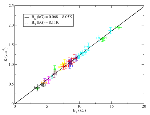
Figure 1 plots the relation between $K$ and $\langle B\rangle$, showing a clear linear relation. The best-fit line (solid black) of all the data suggests that $\langle B\rangle\ {\rm(kG)}=0.068+8.05K$. However, for a star without a magnetic field, in which $K$ is zero, the measured field from the relation should also be zero. Therefore, also shown is the linear fit with the y-intercept forced through the origin (black dashed line). Both lines fit the data equally well; therefore, since the fitted relation should pass through the origin, the latter relation with a zero constant term is adopted with

$$\langle B\rangle\ {\rm(kG)}=8.11K.$$ (3)

This equation is used to calculate the surface magnetic field strength in Table LABEL:results.

4.1 Effects of rotational broadening

The goal of this work is to measure $K$ values for stars with larger $v\sin i$ ($\,\stackrel{{\scriptstyle\raisebox{-0.60275pt}{$\textstyle>$}}}{{\sim}}\,$ 20 km s^-1) in order to estimate $\langle B\rangle$. Therefore, it is important to ascertain how feasible it is to measure magnetic broadening in spectral lines as rotational broadening increases. To investigate this, it is necessary to compare spectra with and without the effects of a magnetic field. zeeman is a fortran program that synthesises stellar spectra and is capable of including the effects of a magnetic field (detailed descriptions of zeeman are provided by Landstreet, 1988; Wade et al., 2001).

zeeman was used to create pairs of synthetic spectra for Fe ii 4520 (with and without the presence of a magnetic field) for incrementally increasing values of $v\sin i$. For this comparison, a field strength of 15 kG was used. The results are shown in Figure 2. One can see how the Zeeman splitting in the Fe ii 4520 line slowly disappears as $v\sin i$ increases, but magnetic broadening still remains. Above about 50 km s^-1, the magnetic broadening is only marginally larger than the rotational broadening. Table LABEL:hwidth lists the FWHD for the lines in Figure 2, with typical uncertainties of order 0.005 Å, as determined from the scatter of multiple measurements. Even for values of $v\sin i$ of about 50 km s^-1, there is still a measurable difference between the rotationally broadened and magnetically and rotationally broadened spectral line of Fe ii at 4520 Å; however, this difference is marginal, suggesting that it may be difficult to obtain an accurate measure of the field above about 50 km s^-1. Note that Fe ii 4520 has a Landé factor $z=1.34$ and that the choice of a different spectral line with a larger $z$ value would increase the difference, perhaps making it plausible to measure the field in stars with even larger rotation rates.

Figure 2: Shown are comparisons between the Fe ii 4520 line for a 15 kG field (black lines) and no magnetic field (red dots) for increasing values of $v\sin i$.

Table 4: Measured full width at half depth (FWHD) for Fe ii 4520 at multiple values of $v\sin i$ for a field strength of 15 kG. Shown are the results without and with a magnetic field and the difference between the two FWHD. The measurements have typical uncertainties of order 0.005 Å.

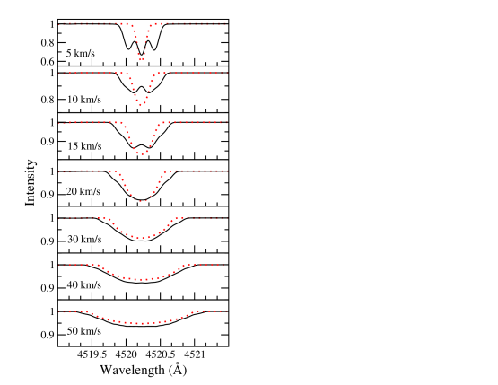
$v\sin i$	FWHD (Å)
(km s-1)	No $B$	$B$	$\Delta$width
5	0.135	0.513	0.378
10	0.234	0.568	0.334
15	0.350	0.580	0.230
20	0.472	0.614	0.142
30	0.720	0.784	0.064
40	0.947	0.981	0.034
50	1.197	1.207	0.010

4.2 Artificial broadening of real spectra

Figure 3: Shown is the difference between the measured and predicted $K$-parameters for three different field strengths at various rotation rates. The actual measurement, when deriving the relation of Equation 2 is also shown. The black circles are for HD 137909 with $\langle B\rangle$ $=5.2$ kG, the blue triangles are for HD 144897 with $\langle B\rangle$ $=9.6$ kG and the red square are for HD 126515 with $\langle B\rangle$ $=15$ kG.

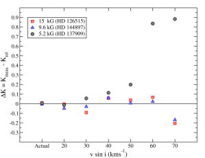
The preceding section suggests that reliably measuring magnetic broadening in a spectral line may be difficult above a rotational velocity of about 50 km s^-1. Therefore, in order to ascertain the reproducibility of the calculated $K$ values at large $v\sin i$, the spectra of three separate stars with field strengths around 5, 10 and 15 kG (HD 137909, HD 144897 and HD 126515, respectively) were convolved with the rotational broadening function (e.g. Unsold, 1955). The spectra were broadened up to 70 km s^-1 in intervals of 10 km s^-1. For each spectrum, the $K$ values were measured in the same manner as described in Section 3. Figure 3 shows the difference between the measured $K$ values and the $K$ value predicted by Equation 2 plotted against $v\sin i$ for the rotationally broadened spectra. Also shown is the actual measurement obtained when deriving the relation.

At both 10 and 15 kG, the $K$ value is consistently reproduced at all $v\sin i$, with a slightly larger disparity at 70 km s^-1 of about 0.2 ${\rm cm^{-1}}$. Above about 50 km s^-1, the $K$ value cannot be reliably measured for a field of about 5 kG. Apparently the marginal difference in the FWHD at larger $v\sin i$ shown in Figure 2 and Table LABEL:hwidth is sufficient to reproduce the measured $K$ value from magnetic broadening for a field above about 10 kG up to about 60 or 70 km s^-1. It is important to note that although Figure 3 suggests that larger magnetic fields follow the linear relationship of Equation 3 above $v\sin i$ of about 50 km s^-1, no a priori knowledge of the field strength will exist when a measurement is made for an actual star. Therefore, for the $v\sin i$’s considered, the method becomes unreliable above about 50 km s^-1 for $\langle B\rangle$ less than or equal to about 15 kG because it is impossible to know whether the measurement yields a reliable $\langle B\rangle$ value or not.

5 Comparison to synthetic spectra

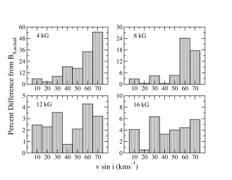
The reproducibility of the $K$ value at large $v\sin i$’s suggests that Equation 3 may be reliably used to estimate the field strengths of magnetic stars that are fast rotators. In Section 4.2, observed spectra were artificially broadened to determine how accurately the $K$ parameter can be reproduced with increasing $v\sin i$. However, the question still remains of how accurate the relation is at measuring the surface field of a star for which the field strength is known precisely. To test this, I used the program zeeman (see Sect. 4). In addition to including the effects of magnetic fields, zeeman also allows as input the specification of a simple magnetic field geometry that is a simple co-axial multipole expansion consisting of dipole, quadrupole and octupole components with the angles between the line-of-sight and rotation axis ($i$) and the magnetic field and rotation axis ($\beta$) specified. As output, zeeman also provides the precise surface field strength. Therefore, it is possible to compare the estimated field strength from Equation 3 to spectra for which the exact field value is known.

Only Fe lines are used to measure $K$ and since the magnetic stars in this study are most certainly Ap in nature, the abundance of Fe was set to a value that is 0.5 dex above the solar ratio. To test the effects of varying geometries, synthetic spectra for $v\sin i$ ’s up to 70 km s^-1 were produced for simple dipolar field strengths of 5, 10, 15 and 20 kG with $i=$ 0, 45 and 90 degrees. To test the applicability of this method of magnetic field determination for increasing $v\sin i$, a geometry where the magnetic field axis is perpendicular to the rotation axis (i.e. $\beta=90^{\circ}$) was favoured, because the angle between the rotation and magnetic field axes are statistically larger in faster rotators (Landstreet & Mathys, 2000). It is recognised that the surface field measured depends not only on the mean value $\langle B\rangle$, but also, to some extent, on the organisation of the field. However, the precision of this method is insufficient to detect these types of changes. As such, the phase dependence in measuring $\langle B\rangle$ with this method is not tested and all computations are performed at the same phase, ensuring that the line-of-sight lies in the plane defined by the rotation and magnetic field axes.

Figure 4 shows the percent difference between the measured $\langle B\rangle$ values from Equation 3 to the actual $\langle B\rangle$ value from the synthetic spectra (as reported by zeeman) plotted against $v\sin i$. The approximate field strength is shown in each panel. Note that no significant differences were found between the three different geometries and therefore only the results for the pole-on geometry are shown. For fields greater than about 12 kG, the predicted field strength from Equation 3 accurately predicts the surface field strength to within 6% at all $v\sin i$ considered. This is also true up to a rotation of 50 km s^-1 for a field of about 8 kG. Above this $v\sin i$, the measured value is within 25% for an 8 kG field. At the lower field strength of 4 kG, the field is predicted within 20% at or below a rotation of 50 km s^-1 and quickly diverges at higher $v\sin i$ values. These results can be understood by considering that at lower field values it becomes increasingly difficult to discern between rotational and magnetic broadening in a spectral line whereas for larger field values the magnetic broadening is still significant compared to the rotational broadening (see Figure 2).

Figure 4: Shown are the percent differences between the measured $\langle B\rangle$ values from Equation 3 to the actual $\langle B\rangle$ value from the synthetic spectra (as reported by zeeman) plotted against $v\sin i$. The approximate field strength is shown in each panel. Note that the y-axis is different for each panel.

6 Conclusions

In this paper, a relation to estimate the surface magnetic field $\langle B\rangle$ for stars with large $v\sin i$ (above about 10 km s^-1) was derived. This was done by extending the work of Preston (1971) to include 102 total spectra for 18 magnetic stars with resolved Zeeman splitting. For each spectrum, the surface field strengths were measured from the observed splitting in Fe ii 6149 and the widths of spectral lines with large and small Landé factors were measured to determine the $K$ parameter (a constant that is proportional to the magnetic field strength). The derived relation is presented in Equation 3.

The $K$ parameter was shown to be reliably reproduced at increasingly large $v\sin i$ when the spectra were rotationally broadened. For lower field values (around 5 kG), the $K$ parameter is not accurately reproduced above about 50 km s^-1.

The relation of Equation 3 was also compared to synthetic spectra for which the surface fields were known precisely. It was found that for $\langle B\rangle$ greater than about 8 kG the field was accurately predicted to within 6% of the actual value. Below about 10 kG, the ability to accurately measure the magnetic field above $v\sin i$ $\simeq 50$ km s^-1 diminishes to within 25% and is completely unreliable for surface fields of order 8 and 4 kG, respectively. Below about 50 km s^-1, a 4 kG field can be measured to within about 20% with increased precision as $v\sin i$ decreases. However, since no knowledge of the surface field strength exists prior to measuring the field from this technique, the method is only useful up to $v\sin i$ of about 50 km s^-1 and for magnetic field strengths down to about 5 kG.

These results are very encouraging and demonstrate that this simple method can reliably estimate the surface field strengths of magnetic stars with large $v\sin i$ (up to about 50 km s^-1). Thus, this technique will allow constraints to be placed on the mean surface field variations of magnetic stars for which only line-of-sight measurements were previously possible.