DESY 14-125
DO-TH 14/15
LPN 14-089
SFB/CPP-14-42
Non-planar Feynman integrals, Mellin-Barnes representations, multiple sums

Abstract:

The construction of Mellin-Barnes (MB) representations for non-planar Feynman diagrams and the summation of multiple series derived from general MB representations are discussed. A basic version of a new package AMBREv.3.0 is supplemented. The ultimate goal of this project is the automatic evaluation of MB representations for multiloop scalar and tensor Feynman integrals through infinite sums, preferably with analytic solutions. We shortly describe a strategy of further algebraic summation.

1 Introduction

There are many methods to calculate Feynman integrals, both numerically and analytically. Here, we follow an attractive method, relying on changing integrals over Feynman parameters into complex path integrals using the Mellin-Barnes (MB) identity [1, 2, 3, 4, 5, 6, 7, 8, 9, 10]. Several talks at this conference are devoted to this subject with different approaches. We refer to [11, 12] where Schwinger’s $\alpha$ representation of Feynman integrals is used for their evaluation with hyperlogarithms (package HyperInt), and to the numerical approach [13, 14] to the Feynman parameter representation with sector decomposition (package SecDec).

Our starting point is the Feynman parameterization for a typical loop momentum integral of the form

$$G(X) = \frac{(-1)^{N_{\nu}}\Gamma\left(N_{\nu}-\frac{d}{2}L\right)}{\prod\limits_{i=1}^{N}\Gamma(n_{i})}\int\prod\limits_{j=1}^{N}dx_{j}~{}x_{j}^{n_{j}-1}\delta(1-\sum\limits_{i=1}^{N}x_{i})\frac{U(x)^{N_{\nu}-d(L+1)/2}}{F(x)^{N_{\nu}-dL/2}}.$$ (1)

Here, $n_{i}$ is the power of inverse propagator $i$, $N_{\nu}=\sum_{i=1}^{N}n_{i}$, $d=4-2\epsilon$, $N$ the number of internal lines and $L$ the number of loops. The functions $U$ and $F$ are called graph or Symanzik polynomials [15, 16, 17] and are composed of the Feynman parameters $x_{i}$ ($U$ and $F$) and of the masses and momenta of the propagators ($F$). The general MB relation can be applied to the polynomials  $U$ and  $F$:

$$\frac{1}{(A_{1}+\ldots+A_{n})^{\lambda}}=\frac{1}{\Gamma(\lambda)}\frac{1}{(2\pi i)^{n-1}}$$ (2)

$$\times \int_{-i\infty}^{i\infty}dz_{1}\ldots dz_{n-1}\prod\limits_{i=1}^{n-1}A_{i}^{z_{i}}~{}A_{n}^{-\lambda-z_{1}-\ldots-z_{n-1}}\times\prod\limits_{i=1}^{n-1}\Gamma(-z_{i})~{}\Gamma(\lambda+z_{1}+\ldots+z_{n-1}).$$

The result are multi-dimensional MB integrals.

The aim of our work is to make the procedure of solving these integrals automatic as much as possible. In general we want to

1. construct MB representations;

2. change them into nested sums;

3. solve the sums numerically or analytically.

Here we discuss shortly some aspects related to these steps. Certainly, there are limitations for the application of the MB method, whose complexity rises with

• the number $L$ of the loops involved;

• the number of scales resulting from up to $N$ different internal masses and $E$ external massive and/or off-shell particles;

• the number $N$ of internal lines;

• the rank $R$ in case of tensor integrals; $R=0$ for scalar integrals.

There are several public software packages for the application of MB integrals in particle physics calculations. On the MB Tools webpage [6] and on the AMBRE webpage [18] there are codes related to the MB approach:

• MB by M. Czakon [7] and MBresolve by V. Smirnov [8] – for the analytic continuation of Mellin-Barnes integrals in $\epsilon$;

• MBasymptotics by M. Czakon ([6], 2005) – for the parametric expansions of Mellin-Barnes integrals;

• barnesroutines by D. Kosower ([6], 2008) – for the automatic application of the first and second Barnes lemmas;

• AMBREv.2.0 [9, 10, 18] – for the creation of (mostly planar) MB representations and later calls of other tools;

• AMBREv.3.0 by I. Dubovyk, J. Gluza, K. Kajda, T. Riemann ([18], 2014) – for the creation of non-planar MB representations up to two loops; the automatic three-loop case is under development.

The AMBRE package generates multiloop scalar and tensor Feynman integrals. For planar cases, the automatic derivation of MB integrals by AMBRE is optimal when using the so-called loop-by-loop approach (LA). An example are the ladder diagrams shown in Fig. 1 and commented in Tab. 1.

In this contribution, we present a new branch of the AMBRE package, AMBREv.3.0 (July 2014). This version may treat also non-planar structures with improved efficiency and may treat up to two loops presently. A global approach (GA) may be chosen where $F$ and $U$ polynomials are changed into MB representations with help of Eq. (2) just in one step. Alternatively, one may choose a hybrid approach which treats planar subloops separately. The procedures are discussed in section 2. For more details on the LA and GA approaches, see [9]. In section 3 a few comments are given on how MB integrals can be changed into nested sums, and how to calculate them. The paper finishes with a summary.

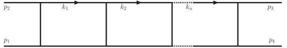
Figure 1: $n$-loop ladder diagram with $k_{1},...,k_{n}$ internal and $p_{1},...,p_{4}$ external momenta.

Dimensions of	Massless  cases				Massive  cases
planar ladder MB integrals
Number of loops ($L$)	1	2	3	4	1	2	3	4
No Barnes First Lemma (BFL)	1	4	7	10	3	8	13	18
With BFL	1	4	7	10	2 (1+1)	6 (4+2)	10 (7+3)	14 (10+4)

Table 1: Optimal results for ladder diagrams defined in Fig. 1: $\rm{Dim(massive~{}case)}=\rm{Dim(massless~{}case)}+\#loops$.

2 Construction of Mellin-Barnes integrals

For non-planar diagrams the GA approach is applied. Further, we use the Cheng–Wu theorem [16, 19] which states that Eq. (1) holds also with the modified $\delta$-function

$$\delta\left(\sum\limits_{i\in\Omega}x_{i}-1\right),$$ (3)

where $\Omega$ is an arbitrary subset of the lines $1,\ldots,L$, when the integration over the rest of the variables, i.e. for $i\notin\Omega$, is extended to the integration from zero to infinity. One can prove this theorem in a simple way starting from the $\alpha$-representation using

$$1=\int\limits_{0}^{\infty}\frac{d\lambda}{\lambda}\delta\left(1-\frac{1}{\lambda}\sum\limits_{i=1}^{N}\alpha_{i}\right)\Leftrightarrow 1=\int\limits_{0}^{\infty}\frac{d\lambda}{\lambda}\delta\left(1-\frac{1}{\lambda}\sum\limits_{i\in\Omega}\alpha_{i}\right)$$ (4)

and changing variables from $\alpha_{i}$ to $\alpha_{i}=\lambda x_{i}$ as shown above.

Let us see how this works in the case of the non-planar massless two-loop box, Fig. 2. This integral was first considered in [5] and the Symanzik polynomials are:

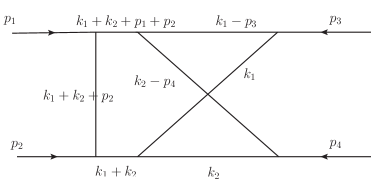
Figure 2: The non-planar massless double box.

$$U(x) = (x_{1}+x_{6})(x_{2}+x_{7})+(x_{3}+x_{4}+x_{5}){(x_{1}+x_{2}+x_{6}+x_{7})},$$ (5)

$$F(x) = -t~{}x_{1}x_{4}x_{7}-u~{}x_{2}x_{4}x_{6}-s~{}x_{1}x_{2}x_{5}-s~{}x_{3}x_{6}x_{7}-s~{}x_{3}x_{5}{(x_{1}+x_{2}+x_{6}+x_{7})}.$$ (6)

The factorizations in $U$ and $F$ are connected with a proper collection of Feynman parameters in front of the variables $k_{1},k_{2}$, as shown schematically in Fig. 3. Next we will apply the Cheng-Wu theorem. Then the integral becomes, after introduction of the $x$ variables:

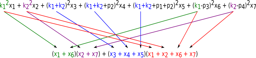
Figure 3: Efficient factorization scheme for the $U$ polynomial.

$$B_{7}^{NP} = \frac{(-1)^{N_{\nu}}\Gamma\left(N_{\nu}-d\right)}{\Gamma(n_{1})\ldots\Gamma(n_{7})}\int\limits_{0}^{\infty}dx_{3}dx_{4}dx_{5}\int\limits_{0}^{1}dx_{1}dx_{2}dx_{6}dx_{7}\prod\limits_{j=1}^{N}~{}x_{j}^{n_{j}-1}\delta[1-{(x_{1}+x_{2}+x_{6}+x_{7})}]$$ (7)

$$\times~{}\frac{((x_{1}+x_{6})(x_{2}+x_{7})+x_{3}+x_{4}+x_{5})^{N_{\nu}-\frac{3d}{2}}}{(-t~{}x_{1}x_{4}x_{7}-u~{}x_{2}x_{4}x_{6}-s~{}x_{1}x_{2}x_{5}-s~{}x_{3}x_{6}x_{7}-s~{}x_{3}x_{5})^{N_{\nu}-d}},$$

and after resolving part of the $F(x)$ by Mellin-Barnes integrals:

$$B_{7}^{NP} = \frac{(-1)^{N_{\nu}}}{\Gamma(n_{1})\ldots\Gamma(n_{7})}\int\limits_{-i\infty}^{i\infty}dz_{1}\ldots dz_{4}\int dx_{1}\ldots dx_{7}\prod\limits_{j=1}^{N}~{}x_{j}^{n_{j}-1}\delta[1-{(x_{1}+x_{2}+x_{6}+x_{7})}]$$ (8)

$$\times~{}(-s)^{-N_{\nu}+d-z_{2}-z_{3}}(-t)^{z_{2}}(-u)^{z_{3}}$$

$${\times~{}\Gamma(-z_{1})\Gamma(-z_{2})\Gamma(-z_{3})\Gamma(-z_{4})\Gamma(N_{\nu}-d+z_{1}+z_{2}+z_{3}+z_{4})}$$

$${\times~{}x_{1}^{-N_{\nu}+d-z_{1}-z_{2}-z_{3}}x_{2}^{z_{2}+z_{3}}{x_{3}}^{-N_{\nu}+d-z_{2}-z_{3}-z_{4}}{x_{4}}^{z_{1}+z_{3}}{x_{5}}^{z_{2}+z_{4}}x_{6}^{z_{1}+z_{2}}x_{7}^{z_{3}+z_{4}}}$$

$$\times~{}[{x_{3}+x_{4}+x_{5}}+(x_{1}+x_{6})(x_{2}+x_{7})]^{N_{\nu}-\frac{3d}{2}}.$$

Now we perform the integrations over Feynman parameters $x_{i}$. In particular, $x_{3},x_{4},x_{5}$ can rather be called Cheng-Wu variables, for which we may use the Beta-function:

$$\int\limits_{0}^{\infty}dx~{}x^{N_{1}}(x+A)^{N_{2}}=\frac{A^{1+N_{1}+N_{2}}\Gamma(1+N_{1})\Gamma(-1-N_{1}-N_{2})}{\Gamma(-N_{2})}.$$ (9)

This, and

$$\int\limits_{0}^{1}\prod_{i}dx_{i}x_{i}^{M_{i}-1}\delta(1-\sum_{i}x_{i})=\frac{\prod_{i}\Gamma(M_{i})}{\Gamma(\sum_{i}M_{i})}$$ (10)

leads finally to the 4-dimensional Mellin-Barnes representation, corresponding, up to some shifts of variables, to Eq. (8) of [5]:

$$B_{7}^{NP} = \frac{(-1)^{N_{\nu}}}{\Gamma(n_{1})\ldots\Gamma(n_{7})}\int\limits_{-i\infty}^{i\infty}dz_{1}\ldots dz_{4}(-s)^{4-2\epsilon-N_{\nu}-z_{23}}(-t)^{z_{3}}(-u)^{z_{2}}$$

$$\times~{}\frac{\Gamma(-z_{1})\Gamma(-z_{2})\Gamma(-z_{3})\Gamma(-z_{4})\Gamma(2-\epsilon-n_{45})\Gamma(2-\epsilon-n_{67})}{\Gamma(4-2\epsilon-n_{4567})\Gamma(n_{45}+z_{1234})\Gamma(n_{67}+z_{1234})\Gamma(6-3\epsilon-N_{\nu})}$$

$$\times~{}\Gamma(n_{2}+z_{23})\Gamma(n_{4}+z_{24})\Gamma(n_{5}+z_{13})\Gamma(n_{6}+z_{34})\Gamma(n_{7}+z_{12})\Gamma^{3}(-2+\epsilon+n_{4567}+z_{1234})$$

$$\times~{}\Gamma(4-2\epsilon-n_{124567}-z_{123})\Gamma(4-2\epsilon-n_{234567}-z_{234})\Gamma(-4+2\epsilon+N_{\nu}+z_{1234}),$$

with notations $z_{i\ldots j\ldots k}=z_{i}+\ldots+z_{j}+\ldots+z_{k}$ and $n_{i\ldots j\ldots k}=n_{i}+\ldots+n_{j}+\ldots+n_{k}$.

In the new version of the AMBRE package, AMBREv.3.0 [20], the procedure is applied properly in an automatic way. The corresponding Mathematica sample file MB_GA_2loopNP_massless.nb with a derivation of Eq. (2) can be found at [18].

In the same way we can use the Cheng-Wu theorem for massless non-planar 3-loop diagrams, e.g. for that shown in Fig. 4. Here we prefer to use a hybrid method. In a first stage, the planar subloop over $k_{1}$ is considered and the corresponding $F$ and $U$ polynomials are changed into MB integrals. Next the non-planar subloop with momenta $k_{2},k_{3}$ is considered using the GA approach for non-planar diagrams. For the planarity identification, i.e. the check whether a diagram is planar or not, the Mathematica package PlanarityTest v.1.1 [21] is used [22]. An example for the hybrid method can be found at the webpage [18], as file MB_hybrid_3loopNP_massless.nb.

In Tables 2 and 3, the numbers of dimensions of the Mellin-Barnes representation for the massive 3-loop cases are shown for the loop-by-loop approach (LA) and for the general approach (GA), respectively. An efficient and satisfactory way to decrease them has not been found so far. More details on the new implementations in the AMBRE package will be described in a forthcoming paper.

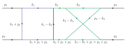
Figure 4: Hybrid method: first $F$ and $U$ polynomials over the ${k_{1}}$-subloop are worked out (planar subgraph), then $\{k_{2},k_{3}\}$ are integrated over (non-planar subgraph).

Massless  case		Massive  case
2-loop	3-loop	2-loop	3-loop
7	10	11	16
6	9	8	12

Table 2: Mellin-Barnes integrals derived by AMBRE. The loop-by-loop approach (LA) is applied: dimensions of some $2\rightarrow 2$ non–planar topologies before and after applying Barnes’ first Lemma. The 2-loop topology corresponds to Fig. 2, while the 3-loop topology corresponds to Fig. 4. Massive case means that the horizontal lines in Figs. 2 and  4 are massive.

Massless case		Massive  case
2-loop	3-loop	2-loop	3-loop
4	7	13	18
4	7	11	15

Table 3: Mellin-Barnes integrals derived by AMBRE. The general approach (GA) is applied. All notations are as in Table 2.

3 Towards summation of iterated integrals

In a second part of our project of developing automatic tools for deriving and solving Mellin-Barnes integrals we explore the general case of deriving multiple sums of residues for Feynman integrals, with the idea then to apply algebraic summation techniques like those developed at the Research Institute for Symbolic Computation (RISC)  [23]. As a first step we prepared an appropriate Mathematica package, MBsums v.0.9 [24].

In the approach to Feynman integrals advocated here, the MB representations can be cast in a general form:

$$\frac{1}{(2\pi i)^{r}}\int\limits_{-i\infty}^{i\infty}\dots\int\limits_{-i\infty}^{i\infty}\underset{i}{\overset{r}{\Pi}}dz_{i}\;{{F}}(Z,X,{\vec{n}},\epsilon)\frac{\underset{j}{\Pi}\;{{G_{j}}}(N_{j})}{\underset{k}{\Pi}\;{{G_{k}}}(N_{k})}.$$ (12)

The integral ranges over $r$ complex variables $z_{i}\in Z$, and the integration path has to be properly chosen. The function $F$ depends on kinematical parameters like $s,t,u$, which are derived from the scalar invariants of the problem, and on internal masses; they are represented by $X$. The indices of the propagators $n_{i}$ constitute ${\vec{n}}=\{n_{1},\ldots,n_{N}\}$, and the dimensional regulator is $\epsilon=2-D/2$.

In practice $F$ is a product of powers of dimensionless parameters $X_{k}$, with exponents being linear combinations of $z_{i},n_{i}$ and $\epsilon$:

$${F}\sim\prod_{k}\;{X}_{k}^{\sum_{i,j}(\alpha_{i}z_{i}+\beta_{j}n_{j}+\gamma\epsilon)},$$ (13)

where the coefficients $\alpha_{i},\beta_{j},\gamma$ are real, $\alpha_{i},\beta_{j},\gamma\in\mathbf{R}$, and the ${X_{k}}$ are composed of ratios of invariants and masses, e.g. ${X_{k}}\in\{\frac{s}{t},\frac{m^{2}}{s},...\}.$ The $\Gamma$-functions $G_{k}(N_{k})$ in Eq. (12) have arguments similar to the exponents occurring in $F$, $N_{k}=\sum_{i,j}(\alpha_{i}z_{i}+\beta_{j}n_{j}+\delta\epsilon)$.

The point is how to evaluate the integral in Eq. (12) exactly or in some approximation, analytically or numerically? Assuming the kinematics to be euclidean or minkowskian, allowing for arbitrary numerics or assuming some small parameters in the set $X$ (see e.g. [25]).

A combined use of AMBRE and MB allows to derive a collection of Mellin-Barnes representations for scalar or tensor Feynman integrals, already regulated in the dimension $D=4-2\epsilon$.

Least problems are faced when seeking some numerical answers for euclidean kinematics. A combined use of AMBRE and MB with a numerical integration package often is applicable. For massless problems, one or the other more or less systematic approach towards analytical solutions is known [26, 27, 28, 11].

For massive, non-planar Feynman integrals however, it is nearly impossible to find complete analytic solutions. Only one of the problems is that MB integrals start to be truly multidimensional.

An immediate method is changing the regulated MB integrals into (usually) infinite series by closing the integration contours in the multi-dimensional complex plane and calculating the sequence of residues. Depending on closing contours to the left or right, convergent infinite series can be obtained which might be suitable for further processing. However, the choice of proper contours depends not only on the general features of the Feynman integral, but also on the values of kinematical parameters. Let us look at the simple one-dimensional integral

$$\int\limits_{-i\infty-1/2}^{i\infty-1/2}dz_{1}(-1/s)^{z_{1}}\frac{\Gamma[-z_{1}]^{3}\Gamma[1+z_{1}]}{\Gamma[-2z_{1}]}$$ (14)

which corresponds (up to a factor) to the coefficient of the $1/\epsilon$ term in the expansion of the massive QED box function. It might look convergent for e.g. $s=-3$ when closing the $z_{1}$ contour to the right and taking residues, but in fact the Gamma functions of the integrand change the sum into a chain of alternating and increasing numbers. The integral converges above the threshold, $|s|>4$, if the contour is closed to the right.

The input function of the Mathematica package MBsums is one of the two following:

$$\verb|MBIntToSum[int,{},contours]|,$$ (15)

$$\verb|MBIntToSum[int,kinematics,contours]|.$$ (16)

Here int is the expression to be evaluated (an output from AMBRE and MB, with or without a dependence on $\epsilon$). The list contours is connected with choices of (i) the order of integrations, and (ii) closing integration contours (to the left (L) or to the right (R)). If the list of kinematics is not empty, the list of contours will be automatically changed by MBsums in order to achieve numerical convergence at the specified kinematical point. For instance, for a two dimensional MB integral which emerges in some massive cases, we have:

$$\verb|int = MBint[((-x)^(z1 - z2) Gamma[1 - z1] Gamma[-z1] |$$ (17)

$$\verb|Gamma[z1] Gamma[1 + z1] Gamma[1 + z1 - z2]^2|$$

$$\verb|Gamma[-z2] Gamma[-z1 + z2])/Gamma[2 + z1 - 2 z2],|$$

$$\verb|{{eps -> 0}, {z1 -> -(13/32), z2 -> -(5/32)}}]|.$$

The corresponding function call might be:

$$\verb|MBIntToSum[int,{x->-1/2},{z2 -> L, z1 -> L}]|.$$ (18)

In this case the output is:

$$\verb|{{((-1)^(-n1 - 2 n2) (-x)^n1 n1! (-1 + n1 + n2)!|$$ (19)

$$\verb|(HarmonicNumber[-1 + n1 + n2]- HarmonicNumber[1 + 2 n1 + n2]))|$$

$$\verb|/(1 + 2 n1 + n2)!, n1 >= 0 && n2 >= 1, {n1, n2}}}|.$$

This expression represents a double sum in $x=-s/m^{2}$, to be summed over non-negative n1 and n2>0. For details see also the sample file LL2014-MBsums.nb at [24].

Here the situation is relatively simple, but more general conditions are possible, e.g.: n1 >= 0 && n2 >= 0 && n1 > n2. Certainly, for higher dimensional integrals, the multiple series will be much more involved, as far as conditional statements for the counting parameters $n_{i}$ are concerned. For a $D$-dimensional multiple integral, the list contours can be given in $D!2^{D}$ different ways, depending on the integration order and on the direction of closing the contours. In the above example, there are eight possible versions. One may try them out and will observe final expressions of rather different complexity; the most efficient one has been shown here. We have no recipe to optimize the program properly in this respect and leave this to the user. Another tricky point for programming was the proper taking into account of multiple residues arising from singularities of several Gamma functions (and their derivatives) at certain values of the summation variables.

After getting proper multiple series, one may proceed with their summation, using advanced summation technologies [29, 30, 31, 32, 33, 34, 35, 36, 37] as encoded in the packages Sigma [38, 39], EvaluateMultiSums, and SumProduction [40, 41, 42].

In fact, compared to the derivation of multiple series, which is at least in principle straightforward, the summation is the much more involved part of the problem. In an ideal world, one has a summation theory at hand which has been solving the summation problem already in generality, and which is made applicable in a computer algebra package.

In our real world, usually we do not have such a theory and/or package.

There are simple cases with known solutions. One of them is the integral in Eq. (14). The corresponding infinite sum may be done just by Mathematica’s built-in function Sum, but also with available packages [43, 44, 45, 46].

In our study of planar massive 2-loop box integrals for Bhabha scattering [25], we could sum up all the infinite sums by XSUMMER [26] after expanding in the small parameter $m_{e}^{2}/s$; the problem became low-dimensional (in fact: factorized into one-dimensional sums) and was solved by simple polylogarithmic functions. In the famous cases of solving the planar and non-planar massless QED double boxes, as well as the planar massive one [47], the authors were able to sum up their expressions until the constant term by dedicated handlings. For the non-planar massive double box, this was already impossible [48].

We do not discuss here some additional numerical treatments. One can try:

1. Write the sum in terms of nested sums using the Mathematica package Sigma [42].

2. Exploit the structure of the sums by recursively applying rewrite rules to generate iterated integrals; see the talk by C. Raab at this conference, [49, 50].

3. Simplify the result to a canonical form, e.g. by using the Mathematica package
   HarmonicSums [51, 52, 53, 54].

More specifically, the aim is to rewrite infinite sums in terms of iterated integrals

$$\sum_{n=0}^{\infty}f(n)x^{n}\quad\rightarrow\quad h_{0}(x)\int_{0}^{x}dt_{1}h_{1}(t_{1})\dots\int_{0}^{t_{k-1}}dt_{k}h_{k}(t_{k})$$ (20)

over a certain alphabet of integrands, which occur in course of a systematic conversion, as e.g.

$$\left\{\frac{1}{t-a},\quad\frac{1}{(t-a)\sqrt{t-b}},\quad\frac{1}{\sqrt{t-b}\sqrt{t-c}},\quad\frac{1}{(t-a)\sqrt{t-b}\sqrt{t-c}}\right\},$$ (21)

with $a,b,c\in\mathbb{R}$.

For instance, in the case of the MB integral in Eq. (17), we have

$$\sum_{n_{2}=0}^{\infty}\sum_{n_{1}=0}^{\infty}\frac{n_{2}!(n_{1}+n_{2})!}{(n_{1}+2n_{2}+2)!}\left(S_{1}(n_{1}+n_{2})-S_{1}(n_{1}+2n_{2}+2)\right)x^{n_{2}},$$ (22)

with $S_{1}(N)=\sum_{k=1}^{N}(1/k)$ the harmonic sum.

So, the steps to be applied are:

1. Compute the inner sum using Sigma [42]:

   $$\sum_{n_{2}=0}^{\infty}\frac{S_{1}(n_{2})-S_{1}(2n_{2}+1)}{(n_{2}+1)(2n_{2}+1)\binom{2n_{2}}{n_{2}}}x^{n_{2}}.$$ (23)

2. Transform the result algorithmically to iterated integrals

   $$\frac{1}{x}\int_{0}^{x}\frac{dt_{1}}{\sqrt{t_{1}}\sqrt{4-t_{1}}}\int_{0}^{t_{1}}\frac{dt_{2}}{\sqrt{t_{2}}\sqrt{4-t_{2}}}\left(-2+\int_{0}^{t_{2}}\frac{dt_{3}}{t_{3}^{3/2}\sqrt{4-t_{3}}}\int_{0}^{t_{3}}\frac{t_{4}dt_{4}}{\sqrt{t_{4}}\sqrt{4-t_{4}}}\right).$$ (24)

3. Convert the integrals to normal form using integrands of the form (21) only,

   $$-\frac{1}{x}\int_{0}^{x}\frac{dt_{1}}{\sqrt{t_{1}}\sqrt{4-t_{1}}}\int_{0}^{t_{1}}\frac{dt_{2}}{t_{2}}\int_{0}^{t_{2}}\frac{dt_{3}}{\sqrt{t_{3}}\sqrt{4-t_{3}}}.$$ (25)

4. In the present simple case one may remove square roots by the transformation $x=-\frac{(1-y)^{2}}{y}$, see e.g. [55], rewrite the result by HarmonicSums [51, 52, 53, 54], and express the final harmonic polylogarithms [56] in terms of the classical polylogarithms

   $$\frac{y}{(1-y)^{2}}\left(4\zeta_{3}+2\zeta_{2}\ln(y)+\frac{\ln(y)^{3}}{6}+2\ln(y)\mathrm{Li}_{2}(y)-4\mathrm{Li}_{3}(y)\right).$$ (26)

In general a much wider class of iterated integrals will occur, see e.g. [50, 57].

We are far from a stage where we might say that a summation procedure exists or where an automatic procedure would apply. It is even unknown in which kind of function space the result of a multiple sum might be found.

But we see from the more developed method of differential equations for solving Feynman integrals that the research field is promising.

4 Summary

The MB approach for the calculation of Feynman diagrams relies on an individual approach to single multi-dimensional complex contour integrals. There are tools which help to solve them, though still not general enough for the massive cases we are interested in. We reported here on some progress in constructing MB representations with a new version of the AMBRE package, being better suited for non-planar Feynman diagrams, and on progress in changing them into suitable multiple sums, which might be further studied aiming at analytic solutions. At the moment the main concern in our investigations focuses on systematic solutions of two- and three-dimensional planar and non-planar MB integrals corresponding to massive Feynman integrals. Using a specific, relatively simple case of a double sum arising from a massless configuration, we sketched the subsequent algebraic treatment with algorithms of summation theory.

References

- [1] E. W. Barnes, A new development of the theory of the hypergeometric functions, Proc. Lond. Math. Soc. (2) 6 (1908) 141–177, http://plms.oxfordjournals.org/content/s2-6/1/141.full.pdf.
- [2] N. Usyukina, On a Representation for Three Point Function, Teor.Mat.Fiz. 22 (1975) 300–306, DOI: 10.1007/BF01037795.
- [3] E. Boos and A. I. Davydychev, A Method of evaluating massive Feynman integrals, Theor.Math.Phys. 89 (1991) 1052–1063, DOI: 10.1007/BF01016805.
- [4] V. Smirnov, Analytical result for dimensionally regularized massless on-shell double box, Phys. Lett. B460 (1999) 397–404, [hep-ph/9905323].
- [5] B. Tausk, Non-planar massless two-loop Feynman diagrams with four on- shell legs, Phys. Lett. B469 (1999) 225–234, [hep-ph/9909506].
- [6] MB Tools webpage http://projects.hepforge.org/mbtools/.
- [7] M. Czakon, Automatized analytic continuation of Mellin-Barnes integrals, Comput. Phys. Commun. 175 (2006) 559–571, [hep-ph/0511200].
- [8] A. V. Smirnov and V. A. Smirnov, On the Resolution of Singularities of Multiple Mellin- Barnes Integrals, Eur. Phys. J. C62 (2009) 445, [0901.0386].
- [9] J. Gluza, K. Kajda, and T. Riemann, AMBRE - a Mathematica package for the construction of Mellin-Barnes representations for Feynman integrals, Comput. Phys. Commun. 177 (2007) 879–893, [0704.2423].
- [10] J. Gluza, K. Kajda, T. Riemann, and V. Yundin, Numerical Evaluation of Tensor Feynman Integrals in Euclidean Kinematics, Eur. Phys. J. C71 (2011) 1516, [1010.1667].
- [11] E. Panzer, Feynman integrals via hyperlogarithms, talk held at Workshop Loops and Legs in Quantum Field Theory, April 27 - May 2, 2014, Weimar, Germany [arXiv:1407.0074]; slides of talk at LL2014 webpage.
-
[12]
E. Panzer, Feynman integrals via hyperlogarithms,
1407.0074. For the package
HyperIntsee [58]. -
[13]
S. Borowka, T. Hahn, S. Heinemeyer, G. Heinrich, and W. Hollik, Momentum-dependent two-loop QCD corrections to the neutral Higgs-boson
masses in the MSSM, 1404.7074. Sector decomposition package
SecDecv.2.2, http://secdec.hepforge.org. - [14] S. Borowka, Momentum-dependent two-loop QCD corrections to the neutral Higgs-boson masses in the MSSM, PoS LL2014 (2014) 033. Slides of talk at LL2014 webpage.
- [15] N. Nakanishi, Parametric integral formulas and analytic properties in perturbation theory, Prog. Theor. Phys. Supplement 18 (1961) 1, http://ptps.oxfordjournals.org/content/18/1.full.pdf.
- [16] N. Nakanishi, Graph Theory and Feynman Integrals. Gordon and Breach, 1971.
- [17] C. Bogner and S. Weinzierl, Feynman graph polynomials, Int. J. Mod. Phys. A25 (2010) 2585–2618, [1002.3458].
-
[18]
I. Dubovyk, J. Gluza, K. Kajda, T. Riemann,
AMBREproject webpage, Silesian Univ., Katowice, http://www.us.edu.pl/~gluza/ambre. - [19] V. Smirnov, Multiloop Feynman integrals, Scholarpedia, 4(6):8507, http://dx.doi.org/10.4249/scholarpedia.8507 (June 23, 2014).
-
[20]
I. Dubovyk, J. Gluza, K. Kajda, T. Riemann, Mathematica package
AMBREv.3.0, webpage http://www.us.edu.pl/~gluza/ambre/. -
[21]
I. Dubovyk and K. Bielas, Mathematica package
PlanarityTest, webpage http://www.us.edu.pl/~gluza/ambre/planarity. - [22] K. Bielas, I. Dubovyk, J. Gluza, and T. Riemann, Some Remarks on Non-planar Feynman Diagrams, Acta Phys. Polon. B44 (2013), no. 11 2249–2255, [1312.5603].
- [23] J. Gluza and T. Riemann, Simple Feynman diagrams and simple sums, Talk held at RISC - DESY Workshop on Advanced Summation Techniques and their Applications in Quantum Field Theory on the occasion of the 5th year jubilee of the RISC-DESY cooperation, May 7-8, 2012, RISC Institute, Castle of Hagenberg, Linz, Austria. Conference link: http://www.risc.jku.at/conferences/RISCDESY12/, talk link: http://www-zeuthen.desy.de/~riemann/Talks/riemann-Linz-2012-05.pdf .
-
[24]
M. Ochman, Mathematica package
MBsums, webpage http://www.us.edu.pl/~gluza/ambre/MBsums. - [25] M. Czakon, J. Gluza, and T. Riemann, The planar four-point master integrals for massive two-loop Bhabha scattering, Nucl. Phys. B751 (2006) 1–17, [hep-ph/0604101].
- [26] S. Moch and P. Uwer, XSummer: Transcendental functions and symbolic summation in Form, Comput. Phys. Commun. 174 (2006) 759–770, [math-ph/0508008].
- [27] F. Brown, The massless higher-loop two-point function, Commun. Math. Phys. 287 (2009) 925–958, [0804.1660].
- [28] C. Anastasiou, C. Duhr, F. Dulat, and B. Mistlberger, Soft triple-real radiation for Higgs production at N3LO, JHEP 1307 (2013) 003, [1302.4379].
- [29] M. Karr, Summation in finite terms, J. ACM 28 (1981) 305–350.
- [30] C. Schneider, Symbolic summation in difference fields, Tech. Rep. 01-17, RISC-Linz, J. Kepler University, November, 2001. PhD Thesis, http://www.risc.jku.at/publications/download/risc_3017/SymbSumTHESIS.pdf.
- [31] C. Schneider, Solving parameterized linear difference equations in terms of indefinite nested sums and products, J. Differ. Equations Appl. 11 (2005) 799–821, DOI: 10.1080/10236190500138262.
- [32] C. Schneider, Simplifying Sums in -Extensions, J. Algebra Appl. 6 (2007) 415–441, DOI: 10.1142/S0219498807002302.
- [33] C. Schneider, A refined difference field theory for symbolic summation, J. Symbolic Comput. 43 (2008) 611–644, [arXiv:0808.2543].
- [34] C. Schneider, Structural Theorems for Symbolic Summation, Appl. Algebra Engrg. Comm. Comput. 21 (2010) 1–32, DOI: 10.1007/s00200–009–0115–3.
- [35] C. Schneider, A Symbolic Summation Approach to Find Optimal Nested Sum Representations, in Motives, Quantum Field Theory, and Pseudodifferential Operators (A. Carey, D. Ellwood, S. Paycha, and S. Rosenberg, eds.), vol. 12 of Clay Mathematics Proceedings, pp. 285–308, Amer. Math. Soc, 2010. arXiv:0808.2543.
- [36] C. Schneider, Parameterized Telescoping Proves Algebraic Independence of Sums, Ann. Comb. 14 (2010) 533–552, [arXiv:0808.2543].
- [37] C. Schneider, Fast Algorithms for Refined Parameterized Telescoping in Difference Fields, in Computer Algebra and Polynomials (M. W. J. Guitierrez, J. Schicho, ed.), Lecture Notes in Computer Science (LNCS), to appear. Springer, 2014. arXiv:1307.7887.
- [38] C. Schneider, Symbolic summation assists combinatorics, Sém. Lothar. Combin. 56 (2007) 1–36, Article B56b, http://www.emis.de/journals/SLC/wpapers/s56.html.
- [39] C. Schneider, Simplifying multiple sums in difference fields, in Computer Algebra in Quantum Field Theory: Integration, Summation and Special Functions (C. Schneider and J. Blümlein, eds.), Texts and Monographs in Symbolic Computation, pp. 325–360. Springer, 2013. arXiv:1304.4134.
- [40] J. Ablinger, J. Blumlein, S. Klein, and C. Schneider, Modern Summation Methods and the Computation of 2- and 3-loop Feynman Diagrams, Nucl.Phys.Proc.Suppl. 205-206 (2010) 110–115, [1006.4797].
- [41] J. Blumlein, A. Hasselhuhn, and C. Schneider, Evaluation of Multi-Sums for Large Scale Problems, PoS RADCOR2011 (2011) 032, [1202.4303].
- [42] C. Schneider, Modern Summation Methods for Loop Integrals in Quantum Field Theory: The Packages Sigma, EvaluateMultiSums and SumProduction, J.Phys.Conf.Ser. 523 (2014) 012037, [1310.0160].
- [43] J. Gluza, F. Haas, K. Kajda, and T. Riemann, Automatizing the application of Mellin-Barnes representations for Feynman integrals, PoS ACAT2007 (2007) 081, [0707.3567].
- [44] T. Huber and D. Maitre, HypExp, a Mathematica package for expanding hypergeometric functions around integer-valued parameters, Comput. Phys. Commun. 175 (2006) 122–144, [hep-ph/0507094].
- [45] T. Huber and D. Maitre, HypExp 2, Expanding Hypergeometric Functions about Half-Integer Parameters, Comput. Phys. Commun. 178 (2008) 755–776, [0708.2443].
- [46] A. I. Davydychev and M. Y. Kalmykov, New results for the epsilon expansion of certain one, two and three loop Feynman diagrams, Nucl.Phys. B605 (2001) 266–318, [hep-th/0012189].
- [47] V. A. Smirnov, Analytical result for dimensionally regularized massive on-shell planar double box, Phys.Lett. B524 (2002) 129–136, [hep-ph/0111160].
- [48] G. Heinrich and V. Smirnov, Analytical evaluation of dimensionally regularized massive on-shell double boxes, Phys. Lett. B598 (2004) 55–66, [hep-ph/0406053].
- [49] J. Ablinger, J. Blümlein, C.G. Raab, C. Schneider, Nested (inverse) binomial sums and new iterated integrals for massive Feynman diagrams, talk held at Workshop Loops and Legs in Quantum Field Theory, April 27 - May 2, 2014, Weimar, Germany; slides of talk at LL2014 webpage.
- [50] J. Ablinger, J. Blümlein, C. Raab, and C. Schneider, Iterated Binomial Sums and their Associated Iterated Integrals, 1407.1822.
- [51] J. Ablinger, A Computer Algebra Toolbox for Harmonic Sums Related to Particle Physics, 1011.1176.
- [52] J. Ablinger, J. Blumlein, and C. Schneider, Harmonic Sums and Polylogarithms Generated by Cyclotomic Polynomials, J. Math. Phys. 52 (2011) 102301, [1105.6063].
- [53] J. Ablinger, J. Blümlein, and C. Schneider, Analytic and Algorithmic Aspects of Generalized Harmonic Sums and Polylogarithms, J. Math. Phys. 54 (2013) 082301, [1302.0378].
- [54] J. Ablinger, Computer Algebra Algorithms for Special Functions in Particle Physics, 1305.0687.
- [55] A. Davydychev and M. Kalmykov, Massive Feynman diagrams and inverse binomial sums, Nucl. Phys. B699 (2004) 3–64, [hep-th/0303162].
- [56] E. Remiddi and J. Vermaseren, Harmonic polylogarithms, Int. J. Mod. Phys. A15 (2000) 725–754, [hep-ph/9905237].
- [57] J. Ablinger and J. Blümlein, Harmonic Sums, Polylogarithms, Special Numbers, and their Generalizations, 1304.7071.
-
[58]
E. Panzer,
HyperIntproject webpage, Humboldt University, Berlin, http://www.math.hu-berlin.de/~panzer/.