Sure Screening for Gaussian Graphical Models

Abstract

We propose graphical sure screening, or GRASS, a very simple and computationally-efficient screening procedure for recovering the structure of a Gaussian graphical model in the high-dimensional setting. The GRASS estimate of the conditional dependence graph is obtained by thresholding the elements of the sample covariance matrix. The proposed approach possesses the sure screening property: with very high probability, the GRASS estimated edge set contains the true edge set. Furthermore, with high probability, the size of the estimated edge set is controlled. We provide a choice of threshold for GRASS that can control the expected false positive rate. We illustrate the performance of GRASS in a simulation study and on a gene expression data set, and show that in practice it performs quite competitively with more complex and computationally-demanding techniques for graph estimation.

1 Introduction

In recent years, graphical modeling has been a topic of great interest in both the scientific and statistical communities. Applications of graphical modeling are widespread, from computer vision to natural language processing to genomics. In particular, in genomics, graphical models have been extensively used to model gene regulatory networks, composed of tens of thousands of genes. It is typically of interest to infer the structure of the graph based on hundreds, or at most thousands, of observations for which gene expression measurements are available. Consequently, the setting is high-dimensional, in the sense that there are many more features than observations.

Consider the random vector $X=(X_{1},\ldots,X_{p})^{T}$, and the conditional dependence graph $\mathcal{G}=(\Gamma,\mathcal{E})$. Here $\Gamma=\{1,\dots,p\}$ is the set of nodes, and $\mathcal{E}$ is the set of edges in $\Gamma\times\Gamma$. A pair $(a,b)$ is contained in the edge set $\mathcal{E}$ if and only if $X_{a}$ is conditionally dependent on $X_{b}$, given all remaining variables $X_{\Gamma\backslash\{a,b\}}=\{X_{k};k\in\Gamma\backslash\{a,b\}\}$.

The conditional dependence graph takes a particularly simple form if we suppose that $X\sim N({0},{\bf\Sigma})$, where $\bf\Sigma$ is a non-singular covariance matrix. In this setting, a pair of variables is conditionally independent if and only if the corresponding entry of the precision matrix ${\bf\Sigma}^{-1}$ equals zero (Lauritzen,, 1996; Mardia et al.,, 1980). Consequently, in the Gaussian graphical model, recovering the edge set $\mathcal{E}$ is equivalent to recovering the sparsity pattern of the precision matrix ${\bf\Sigma}^{-1}$.

Recently, much attention has been devoted to the task of estimating and recovering the sparsity pattern of a large sparse precision matrix; we provide a brief review of the literature here. A number of authors have considered an $\ell_{1}$-penalized likelihood approach in order to estimate a sparse precision matrix (Yuan and Lin,, 2007; Friedman et al.,, 2008; Rothman et al.,, 2008; Ravikumar et al.,, 2009). To ameliorate the bias incurred by the use of an $\ell_{1}$ penalty, Lam and Fan, (2009) considered the use of a non-convex SCAD penalty. Others have considered a neighborhood selection approach, which entails performing a sparse regression of each variable on all of the other variables in order to estimate the precision matrix (Meinshausen and Bühlmann,, 2006; Yuan,, 2010; Cai et al.,, 2011, 2012; Sun and Zhang,, 2012). Yuan, (2010) considered a Dantzig-type neighborhood selection approach. For many of the aforementioned approaches, statistical convergence results (in terms of various matrix norms) have been established for the high-dimensional setting.

Although various computationally efficient algorithms for estimating a sparse precision matrix have been proposed (see e.g. Friedman et al.,, 2008; Witten et al.,, 2011), the required computations can be burdensome when the number of variables is in the tens of thousands, or even higher. For example, the precision matrix for a problem with $p=25,000$ (the number of genes in the human genome) involves upwards of 300,000,000 parameters. In such a setting, existing algorithms tend to be infeasible. We are thus motivated to consider a computationally-efficient screening approach for Gaussian graphical models that possesses desirable statistical properties.

In recent years, computationally simple variable screening approaches have gained popularity in the context of high-dimensional modeling. Fan and Lv, (2008) proposed the sure independence screening method for linear models. This approach possesses the sure screening property: with probability going to one, all of the important variables will be selected. Fan et al., (2009) and Fan and Song, (2010) extended this approach to the context of generalized linear models. Other marginal screening methods include tilting methods (Hall et al.,, 2009), generalized correlation screening (Hall and Miller,, 2009), nonparametric screening (Fan et al.,, 2011), partial likelihood screening (Zhao and Li,, 2012), and robust rank correlation based screening (Li et al.,, 2012; Zhu et al.,, 2011). Most of the existing screening methods aim to select variables by ranking utilities such as the Pearson’s correlation between the marginal covariates and the response, where variables with strong marginal utilities are selected.

In this paper, we propose a novel screening procedure for recovering the structure of a Gaussian graphical model. We call this approach graphical sure screening (GRASS). Our approach is motivated by the fact that the $a$th column of the precision matrix ${\bf\Sigma}^{-1}$ can be obtained by regressing the $a$th feature onto the $p-1$ other features (Mardia et al.,, 1980). This suggests that in order to estimate $\mathcal{E}_{a}$, the neighbourhood of the $a$th node, we can emulate the sure screening procedure of Fan and Lv, (2008) for linear models: we simply threshold the sample correlations of the $a$th feature with the $p-1$ other features. We show that under certain simple assumptions, the set of nodes for which the sample correlation with the $a$th node exceeds some threshold is guaranteed to contain the true neighborhood, $\mathcal{E}_{a}$, with very high probability. This property holds when the dimension $p$ grows as an exponential function of the sample size $n$. Furthermore, we establish a surprising connection between GRASS and existing approaches for sparse precision matrix estimation using an $\ell_{1}$-penalized log likelihood.

As far as we know, this work is the first time that a sure screening procedure has been applied in an unsupervised context. The proposed method is conceptually very simple, and can be easily implemented in very high dimensions. In contrast to existing methods for estimating a sparse precision matrix, which typically require $\mathcal{O}(p^{3})$ computations (Friedman et al.,, 2008), our procedure requires only $\mathcal{O}(p^{2})$ operations, and hence can be easily scaled to large-$p$ settings.

The rest of this article is organized as follows. In Section 2, we present the GRASS procedure. In Section 3, we establish the theoretical properties for GRASS; these include the sure screening property, size control of the selected edge set, and control of the theoretical false positive rate. A surprising connection between GRASS and existing $\ell_{1}$-penalized approaches for sparse precision matrix estimation is explored in Section 4. Simulation studies are presented in Section 5, and a real data application is in Section 6. We close with a discussion in Section 7.

2 Graphical Sure Screening

Consider the random vector $X=(X_{1},\ldots,X_{p})^{T}\sim N_{p}(0,{\bf\Sigma})$, where $\bf\Sigma$ has unit diagonals, i.e. $\mbox{E}(X_{a}^{2})=1$ for all $a=1,\ldots,p$. The $n\times p$ data matrix ${\bf X}=\left({\bf X}_{1},\cdots,{\bf X}_{p}\right)$ contains $n$ i.i.d. draws from $X$. Let $\gamma_{n}>0$ be some pre-specified threshold.

We propose to obtain a candidate edge set, $\widehat{\mathcal{E}}_{\gamma_{n}}$, and a candidate neighbourhood for the $a$th node, $\widehat{\mathcal{E}}_{a,\gamma_{n}}$, by thresholding the sample correlation matrix by $\gamma_{n}$. That is, we define

$$\widehat{\mathcal{E}}_{\gamma_{n}} = \{(a,b):a<b,|\bm{X}_{a}^{T}\bm{X}_{b}|/n>\gamma_{n}\},$$ (2.1)

$$\widehat{\mathcal{E}}_{a,\gamma_{n}} = \{b:b\neq a,|\bm{X}_{a}^{T}\bm{X}_{b}|/n>\gamma_{n}\}.$$ (2.2)

We refer to (2.1) and (2.2) as the graphical sure screening (GRASS) estimates.

We will show in Section 3 that for an appropriate choice of $\gamma_{n}$, ${\mathcal{E}}_{a}$ is contained in $\widehat{\mathcal{E}}_{a,\gamma_{n}}$ with very high probability, when $p$ grows exponentially with $n$. We refer to this as the sure screening property for the graphical model. This property holds even when the size of the selected neighbourhood is a polynomial order of the sample size, leading to a drastic decrease in the dimension. Furthermore, under certain conditions, GRASS can also control the false positive rate.

3 Theoretical Properties

Here we present some theoretical properties of the GRASS procedure. Proofs are in the Appendix. In what follows, we use the notation $\sigma_{ab}\equiv\mbox{E}(X_{a}X_{b})$.

To begin, we introduce an assumption on the minimum correlation between two nodes connected by an edge.

Assumption 1.

For some constants $C_{1}>0$ and $0<\kappa<1/2$,

$$\mathop{\mathrm{min}}_{(a,b)\in\mathcal{E}}|\sigma_{ab}|\geq C_{1}n^{-\kappa}.$$

Assumption 1 allows us to establish the sure screening property of GRASS, which is presented in Theorem 1.

Theorem 1.

Assume that Assumption 1 holds, and that $\mathrm{log}(p)=C_{3}n^{\xi}$ for some constants $C_{3}>0$ and $\xi\in(0,1-2\kappa)$. Let $\gamma_{n}=2/3C_{1}n^{-\kappa}$. Then, there exist constants $C_{4}$ and $C_{5}$ such that

$$P(\mathcal{E}\subseteq\widehat{\mathcal{E}}_{\gamma_{n}}) {\geq} 1-C_{4}\mathrm{exp}(-C_{5}n^{1-2\kappa}),~{}\mathrm{and}$$

$$P(\mathcal{E}_{a}\subseteq\widehat{\mathcal{E}}_{a,\gamma_{n}}) {\geq} 1-C_{4}\mathrm{exp}(-C_{5}n^{1-2\kappa}).$$

Theorem 1 guarantees that with very high probability, the true edge set is contained in $\widehat{\mathcal{E}}_{\gamma_{n}}$, the edge set estimate from the GRASS procedure. In other words, with very high probability, GRASS will not result in false negatives. This raises the following question: how large is $\widehat{\mathcal{E}}_{a,\gamma_{n}}$, the estimated neighbourhood for the $a$th node? In order to answer this question, we must first introduce an additional assumption.

Assumption 2.

There exist constants $\tau\geq 0$ and $C_{2}>0$ such that

$$\lambda_{\mathrm{max}}({\bf\Sigma})\leq C_{2}n^{\tau},$$

where $\lambda_{\mathrm{max}}({\bf\Sigma})$ is the maximal eigenvalue of ${\bf\Sigma}$.

Assumption 2 indicates that the largest eigenvalue of the population covariance matrix ${\bf\Sigma}$ is allowed to diverge as $n$ grows; however, it cannot diverge too quickly. This condition naturally appears in many applications. For example, it holds for the covariance matrix of a stationary time series (Fan and Lv,, 2008).

We now present Theorem 2, which allows us to control the size of $\widehat{\mathcal{E}}_{a,\gamma_{n}}$.

Theorem 2.

Let $\gamma_{n}=2/3C_{1}n^{-\kappa}$. Under Assumptions 1-2, if $log(p)=C_{3}n^{\xi}$, for $\xi\in(0,1-2\kappa)$, then

$$P\left[|\widehat{\mathcal{E}}_{a,\gamma_{n}}|\leq O(n^{2\kappa+\tau})\right]\geq 1-C_{4}\mathrm{exp}(-C_{5}n^{1-2\kappa}),$$

where the constants $C_{4}$ and $C_{5}$ are as in Theorem 1.

Next we propose a choice of $\gamma_{n}$ that allows us to control the expected false positive rate at a prespecified value. The false positive rate is defined as

$$\frac{|\widehat{\mathcal{E}}_{\gamma_{n}}\cap\mathcal{E}^{c}|}{|\mathcal{E}^{c}|}.$$

We would like the false positive rate to decrease to 0 as $p_{n}$ increases with $n$. As in Zhao and Li, (2012), we do this by first fixing the number of false positives $f$ that we are willing to tolerate; this corresponds to a false positive rate of $f/|\mathcal{E}^{c}|$. In order to control the expected false positive rate, we introduce an additional assumption.

Assumption 3.

For the same $\xi$ as in Theorem 1,

$$\mathop{\mathrm{max}}_{(a,b)\not\in\mathcal{E}}|\sigma_{ab}|=o(n^{-\frac{1-\xi}{2}}).$$

Theorem 3.

Under Assumptions 1-3, if $\log(p)=C_{3}n^{\xi}$ for $\xi$ as in Theorem 1, then we can control the asymptotic expected false positive rate at $f/|\mathcal{E}^{c}|$ by choosing $\gamma_{n}=\Phi^{-1}(1-\frac{f}{p(p-1)})/\sqrt{n}$. Furthermore, with this threshold, the sure screening property of Theorem 1 still holds.

4 Connection with the Graphical Lasso

In recent years, many quite sophisticated approaches for obtaining a sparse estimate of ${\bf\Sigma}^{-1}$ have been proposed. Perhaps the best-known among these is the graphical lasso (Friedman et al.,, 2008; Yuan and Lin,, 2007), which is the solution to the optimization problem

$$\mbox{maximize}_{\bf\Theta}\{\log\det{\bf\Theta}-\mbox{trace}(({\bf X}^{T}{\bf X}/n){\bf\Theta})-\lambda\sum_{i\neq j}|\Theta_{ij}|\}.$$ (4.1)

Recently, Witten et al., (2011) and Mazumder and Hastie, (2012) established a surprising result: the connected components of the graphical lasso estimator are exactly the same as the connected components that result from hard-thresholding the matrix ${\bf X}^{T}{\bf X}/n$ by $\lambda$. In other words, the connected components of the graphical lasso estimator are the same as the connected components of the GRASS edge set estimate, $\widehat{\mathcal{E}}_{\gamma_{n}}$, when $\gamma_{n}=\lambda$.

Does this mean that GRASS and the graphical lasso are identical? Not quite. Though the connected components of the graphical lasso and of GRASS are the same, their entire sparsity patterns are, in general, not the same. The graphical lasso can be thought as a two-stage procedure, in which we first perform GRASS with $\gamma_{n}=\lambda$, and then perform a smaller graphical lasso problem on each connected component of $\widehat{\mathcal{E}}_{\gamma_{n}}$.

Under a set of assumptions explored by Ravikumar et al., (2011), the graphical lasso is known to be model selection consistent. Since the connected components of GRASS and the connected components of the graphical lasso are the same provided that $\gamma_{n}=\lambda$, this means that the model selection consistency results of Ravikumar et al., (2011) are inherited by the connected components of GRASS. In other words, the connected components of GRASS are selected consistently.

5 Simulation Studies

5.1 Data Generation

Let $p$ denote the number of features, and $n$ the number of observations. We considered three ways of generating the edge set $\mathcal{E}$:

• For all $i<j$, we set $(i,j)\in\mathcal{E}$ with probability $0.01$.

• We partitioned the $p$ features into $10$ equally-sized and non-overlapping sets: $C_{1}\cup C_{2}\cup\ldots\cup C_{10}=\{1,\ldots,p\}$, $|C_{k}|=p/10$, $C_{k}\cap C_{j}=\emptyset$. For all $i\in C_{k},j\in C_{k},i<j$, we set $(i,j)\in\mathcal{E}$.

• For $|i-j|\leq 2$ we set $(i,j)\in\mathcal{E}$. Otherwise, $(i,j)\notin\mathcal{E}$.

Once the edge set $\mathcal{E}$ was generated, we created a precision matrix via the following steps:

• Step 1: We generated a $p\times p$ matrix $\bf A$, where

  $$A_{ij}=A_{ji}=\begin{cases}1&\mathrm{\;for\;}i=j\\ \mathrm{Unif}[-0.3,0.7]&\mathrm{\;for\;}(i,j)\in\mathcal{E}\\ 0&\mathrm{\;otherwise}\end{cases}.$$

• Step 2: We created a positive definite matrix ${\bf\Sigma}^{-1}$:

  $${\bf\Sigma}^{-1}={\bf A}+(0.1-\lambda_{\min}({\bf A})){\bf I},$$

  where $\lambda_{\min}(\bf A)$ denotes the smallest eigenvalue of $\bf A$, and $\bf I$ denotes the $p\times p$ identity matrix.

Then the covariance matrix $\bf\Sigma$ was rescaled to have diagonal elements equal to 1. Finally, we generated $n$ observations i.i.d. from a $N(0,{\bf\Sigma})$ distribution.

5.2 Control of False Positive Rate

Theorem 3 states that under certain conditions, performing GRASS with $\gamma_{n}=\frac{1}{\sqrt{n}}\Phi^{-1}(1-q/2)$ leads to control of the expected false positive rate (FPR) at level $q\equiv f/|\mathcal{E}^{c}|$. We now investigate the extent to which GRASS controls the FPR in practice. Results for Simulations A-C are shown in Table 1.

Assumption 3, required for Theorem 3 to hold, states that $\max_{(a,b)\notin\mathcal{E}}|\sigma_{ab}|\rightarrow 0$ as $n\rightarrow\infty$. Simulation B satisfies this assumption, since ${\bf\Sigma}^{-1}$ is block diagonal with completely dense blocks (and thus the same is true of $\bf\Sigma$). As expected, the FPR is controlled successfully in Simulation B (Table 1).

However, Assumption 3 seems not to be satisfied by Simulations A and C. But Table 1 reveals that the FPR is approximately controlled in these settings, especially for larger values of $q$. How can this be?

In order to investigate this, we consider the off-diagonal elements of ${\bf\Sigma}^{-1}$ and $\bf\Sigma$ under Simulations A-C. These are displayed in Figure 1. We see that even for Simulations A and C, the vast majority of the large off-diagonal elements of ${\bf\Sigma}$ correspond to non-zero elements of ${\bf\Sigma}^{-1}$.

Furthermore, in Simulation A, there is a very pronounced relationship between the values of the non-zero elements of ${\bf\Sigma}^{-1}$, and the corresponding values of $\bf\Sigma$. This is the case because in Simulation A, ${\bf\Sigma}^{-1}$ was generated to be so sparse (Section 5.1) that, with high probability, a given column of ${\bf\Sigma}^{-1}$ contains no more than one non-zero off-diagonal element. Consequently, ${\bf\Sigma}^{-1}$ is (approximately) a block-diagonal matrix with blocks containing no more than two features. And consequently the sparsity patterns of ${\bf\Sigma}^{-1}$ and ${\bf\Sigma}$ are almost identical. Furthermore, there is a simple monotone relationship between most of the non-zero elements of the two matrices, which can be easily derived using the standard formula for the inverse of a $2\times 2$ matrix.

Simulation A                           Simulation B                           Simulation C

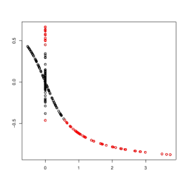
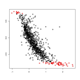
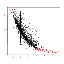
Figure 1: For Simulations A-C with $n=100$ and $p=50$, the off-diagonal elements of ${\bf\Sigma}^{-1}$ (x-axis) and $\bf\Sigma$ (y-axis) are shown. The $0.5$% of largest absolute off-diagonal elements of $\bf\Sigma$ are shown in red; the rest are in black. For all three setups, the vast majority of large off-diagonal elements of $\bf\Sigma$ correspond to non-zero elements of ${\bf\Sigma}^{-1}$. The pronounced relationships seen for Simulation A are due to the extreme sparsity of ${\bf\Sigma}^{-1}$, as is discussed in the text.

			Simulation A			Simulation B			Simulation C
$n$	$p$	$q$	$|\widehat{\mathcal{E}}_{\gamma_{n}}|$	FPR	FNR	$|\widehat{\mathcal{E}}_{\gamma_{n}}|$	FPR	FNR	$|\widehat{\mathcal{E}}_{\gamma_{n}}|$	FPR	FNR
100	50	1e-04	14.504	0.001	0.512	69.816	0	0.652	80.696	0.008	0.674
		0.001	19.664	0.003	0.449	88.496	0.001	0.572	108.496	0.013	0.592
		0.01	46.36	0.013	0.353	131.688	0.011	0.464	168.016	0.03	0.485
		0.1	268.88	0.103	0.23	368.064	0.102	0.305	424.048	0.13	0.322
		0.2	513.632	0.204	0.186	603.432	0.201	0.239	664.824	0.231	0.255
		0.3	752.048	0.302	0.148	834.808	0.299	0.194	893.064	0.328	0.207
		0.5	1236.6	0.501	0.094	1296.344	0.499	0.126	1341.68	0.52	0.135
100	200	1e-04	150.664	0.001	0.73	510.384	0	0.867	247.328	0.001	0.741
		0.001	252.704	0.003	0.651	798.528	0.001	0.802	383.824	0.003	0.656
		0.01	737.752	0.014	0.541	1572.592	0.011	0.691	907.264	0.014	0.54
		0.1	4499.056	0.108	0.363	5599.04	0.101	0.485	4661.928	0.107	0.361
		0.2	8465.392	0.208	0.286	9539.712	0.2	0.388	8608.848	0.206	0.284
		0.3	12405.288	0.307	0.234	13385	0.3	0.318	12516.648	0.305	0.23
		0.5	20233.504	0.505	0.153	20976.56	0.499	0.21	20310.848	0.503	0.151
1000	50	1e-04	27.6	0.003	0.187	154.344	0	0.229	244.904	0.043	0.243
		0.001	31.32	0.004	0.162	163.584	0.001	0.193	274.416	0.053	0.203
		0.01	55.016	0.014	0.129	191.912	0.01	0.15	332.968	0.075	0.158
		0.1	275.04	0.104	0.084	403.752	0.099	0.095	580.152	0.18	0.101
		0.2	518.92	0.204	0.063	634.128	0.2	0.074	803.496	0.277	0.08
		0.3	760.016	0.304	0.053	862.064	0.3	0.06	1016.936	0.37	0.063
		0.5	1244.624	0.503	0.034	1313.84	0.498	0.039	1430.144	0.552	0.042
1000	200	1e-04	586.24	0.008	0.276	2303.16	0	0.395	855.904	0.007	0.279
		0.001	720.152	0.011	0.233	2553.112	0.001	0.338	992.496	0.01	0.237
		0.01	1238.992	0.023	0.184	3149.528	0.01	0.266	1494.464	0.022	0.186
		0.1	4992.952	0.118	0.118	6753.224	0.1	0.171	5181.096	0.115	0.118
		0.2	8946.776	0.218	0.093	10497.4	0.2	0.133	9094.128	0.215	0.092
		0.3	12846.408	0.317	0.076	14198.992	0.3	0.108	12970.448	0.314	0.074
		0.5	20578.888	0.513	0.05	21534.512	0.5	0.07	20659.576	0.51	0.049

Table 1: The false positive rate (FPR; defined as FP/(FP+TN)) and false negative rate (FNR; defined as FN/(TP+FN)) are reported for various values of $q$, the level of desired FPR control. Results for two values of $n$ and $p$, and for each of Simulations A-C, are reported. The value of $|\widehat{\mathcal{E}}_{\gamma_{n}}|$ — the number of elements in the GRASS estimate corresponding to the value of $q_{n}$ — is also reported. Results are averaged over 250 simulated data sets.

5.3 Comparison to Existing Approaches

We now compare the performances of the graphical lasso (Friedman et al.,, 2008), neighborhood selection (Meinshausen and Bühlmann,, 2006), and GRASS on Simulations A-C, with $n=50$ and $p=200$. Results are displayed in Figure 2.

In Simulation B, recall that the sparsity patterns of $\bf\Sigma$ and ${\bf\Sigma}^{-1}$ are identical. In this setting, GRASS outperforms the graphical lasso and neighborhood selection, since it correctly assumes that the sparsity patterns of the covariance and precision matrices are similar. In Simulations A and C, even though this assumption does not hold exactly, the performance of GRASS is quite competitive.

Overall, in Figure 2, there is little difference in performance between GRASS, neighbourhood selection, and the lasso. That is, even though GRASS is an extremely simple approach, in practice GRASS performs competitively with specialized and computationally-intensive procedures for estimating a precision matrix.

Figure 3 displays the adjacency matrices corresponding to the true edge set, as well as the edge sets estimated using the graphical lasso and GRASS, for Simulations B and C. We find once again that the edge sets estimated by the graphical lasso and GRASS appear to be quite similar.

Simulation A                           Simulation B                           Simulation C

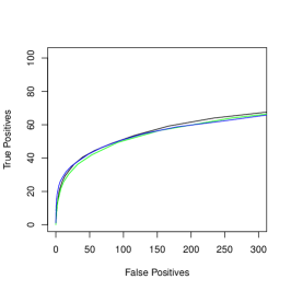
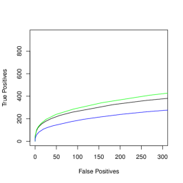
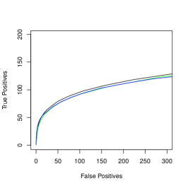
Figure 2: For Simulations A-C with $p=200$ and $n=50$, the number of false and true positive edges detected is displayed as the tuning parameter is varied. Results are shown for graphical lasso (—), neighborhood selection (—), and GRASS (—).

(a)                                        (b)                                        (c)
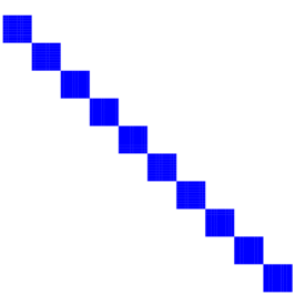
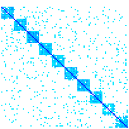
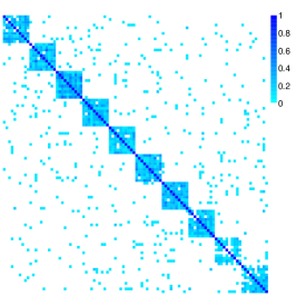
(d)                                        (e)                                        (f)

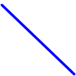
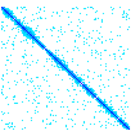
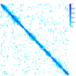
Figure 3: For Simulations B (panels (a)-(c)) and C (panels (d)-(f)) with $p=100$ and $n=50$, the adjacency matrices corresponding to the true edge set (panels (a) and (d)), the graphical lasso estimate (panels (b) and (e)), and the GRASS estimate (panels (c) and (f)) are shown. The adjacency matrices for graphical lasso and GRASS are averaged over 10 simulated data sets; the color of a particular cell in the heatmap corresponds to the fraction of these 10 data sets for which the corresponding edge is estimated to be present. Results for Simulation A are not shown, since in that setting the true edge set is not fixed across the simulated data sets.

6 Analysis of Gene Expression Data

We examined a gene expression data set from Spira et al., (2007), previously studied in Danaher et al., (2013), and publicly available from the Gene Expression Omnibus (Barrett et al.,, 2007) at accession number GDS2771. The data consist of 22,283 microarray-derived gene expression measurements from large airway epithelial cells sampled from 97 patients with lung cancer and 90 controls. We limited our analysis to the 1,778 genes with the highest marginal variance. Each feature was standardized within each class, in order to have mean zero and standard deviation one among the cancer samples, and among the controls.

Our goal is to compare the performances of GRASS and graphical lasso in terms of edge set recovery. Unfortunately, as is typically the case for a high-dimensional biological data set, the true underlying conditional dependence relationships in this data are unknown. In other words, no gold standard is available.

Given the absence of a gold standard, we took the following approach. We split the control samples into two equally-sized sets, Set 1 and Set 2. We applied both graphical lasso and GRASS to each set. We refer to the resulting estimated edge sets as $\widehat{\mathcal{E}}_{1}^{\mathrm{GL}}$, $\widehat{\mathcal{E}}_{1}^{\mathrm{GRASS}}$, $\widehat{\mathcal{E}}_{2}^{\mathrm{GL}}$, and $\widehat{\mathcal{E}}_{2}^{\mathrm{GRASS}}$; tuning parameters were chosen such that $|\widehat{\mathcal{E}}_{1}^{\mathrm{GL}}|=|\widehat{\mathcal{E}}_{2}^{\mathrm{GL}}|=|\widehat{\mathcal{E}}_{1}^{\mathrm{GRASS}}|=|\widehat{\mathcal{E}}_{2}^{\mathrm{GRASS}}|$. In order to quantify the accuracy of the edges estimated on Set 2 by GRASS and the graphical lasso, we first treated the edges estimated by the graphical lasso on Set 1 as the gold standard, and then we treated the edges estimated by GRASS on Set 1 as the gold standard. In greater detail, we calculated:

1. Accuracy of GRASS on Set 2 when graphical lasso on Set 1 is treated as the gold standard. This is calculated as

   $$\left|\widehat{\mathcal{E}}_{1}^{\mathrm{GL}}\cap\widehat{\mathcal{E}}_{2}^{\mathrm{GRASS}}\cap\left(\widehat{\mathcal{E}}_{2}^{\mathrm{GL}}\right)^{c}\right|.$$

2. Accuracy of graphical lasso on Set 2 when graphical lasso on Set 1 is treated as the gold standard. This is calculated as

   $$\left|\widehat{\mathcal{E}}_{1}^{\mathrm{GL}}\cap\widehat{\mathcal{E}}_{2}^{\mathrm{GL}}\cap\left(\widehat{\mathcal{E}}_{2}^{\mathrm{GRASS}}\right)^{c}\right|.$$

3. Accuracy of GRASS on Set 2 when GRASS on Set 1 is treated as the gold standard. This is calculated as

   $$\left|\widehat{\mathcal{E}}_{1}^{\mathrm{GRASS}}\cap\widehat{\mathcal{E}}_{2}^{\mathrm{GRASS}}\cap\left(\widehat{\mathcal{E}}_{2}^{\mathrm{GL}}\right)^{c}\right|.$$

4. Accuracy of graphical lasso on Set 2 when GRASS on Set 1 is treated as the gold standard. This is calculated as

   $$\left|\widehat{\mathcal{E}}_{1}^{\mathrm{GRASS}}\cap\widehat{\mathcal{E}}_{2}^{\mathrm{GL}}\cap\left(\widehat{\mathcal{E}}_{2}^{\mathrm{GRASS}}\right)^{c}\right|.$$

Note that in calculating these accuracies, we only considered feature pairs $(i,j)$ for which GRASS and graphical lasso disagree over whether an edge is present in Set 2 (since feature pairs for which graphical lasso and GRASS agree on Set 2 are uninformative for our purposes).

The results, averaged over 20 splits of the data into Set 1 and Set 2, are summarized in Table 2. They indicate that regardless of whether graphical lasso or GRASS on Set 1 is treated as the gold standard, the results obtained by GRASS on Set 2 have better agreement with the gold standard than do the results obtained by the graphical lasso on Set 2. In other words, independent data provides greater evidence for edges estimated by GRASS than for edges estimated by the graphical lasso, regardless of whether the independent data is evaluated using GRASS or the graphical lasso.

	GRASS as Gold Standard		Graphical Lasso as Gold Standard
$|\widehat{\mathcal{E}}|$	GRASS Accuracy	GL Accuracy	GRASS Accuracy	GL Accuracy
47371.8 (2387.7)	3368.2 (284.6)	1663 (185.4)	2248.7 (85.9)	1824 (64.5)
40781.3 (2346.6)	2307.4 (226.9)	1222.8 (154.8)	1562.5 (68)	1207 (45.7)
33555.9 (2229.2)	1433.4 (165.4)	808.3 (119)	968.5 (48.5)	714.5 (31.4)
25942.8 (2012.8)	783.4 (108.6)	472.8 (82.5)	523.4 (27.3)	373.1 (17.4)
18540.5 (1688.2)	359.4 (60)	227 (47.5)	232.6 (14.9)	155.4 (8.7)
11903.3 (1276.8)	133.4 (24.6)	94 (22.1)	81.6 (5.5)	58.2 (3.7)
6647.9 (834.5)	41.2 (9.7)	26.4 (9.1)	23.6 (2)	12.7 (1.3)
3095.2 (447.3)	6.2 (2)	5.5 (1.8)	2.9 (0.4)	2.1 (0.3)
1142 (184.7)	1.1 (0.3)	0.7 (0.5)	0.5 (0.2)	0.1 (0.1)
312.9 (52.1)	0.2 (0.1)	0 (0)	0 (0)	0 (0)

Table 2: Mean (and standard error) of accuracy of graphical lasso (GL) and GRASS on gene expression data, over 20 splits of the observations into Set 1 and Set 2. $|\widehat{\mathcal{E}}|$, the size of the estimated edge set, is also reported. Regardless of whether GRASS or graphical lasso is treated as the gold standard, GRASS yields more accurate edge set recovery than does the graphical lasso. These results are based on an analysis of the control observations. Similar results are obtained from the cases (results not shown).

7 Discussion

In this paper, we have proposed graphical sure screening (GRASS), a simple and efficient procedure for recovering the structure of a high-dimensional Gaussian graphical model. GRASS is a natural extension of sure screening approaches from the regression and classification frameworks into the setting of Gaussian graphical modeling.

The theoretical results presented in Section 3 for GRASS require a very simple set of assumptions. In particular, Assumption 1, which guarantees that the covariance corresponding to an edge in the graph is not too small, suffices to ensure that GRASS has the sure screening property: that is, GRASS can dramatically reduce the size of the potential edge set while still containing the true edge set with probability tending to one. Unlike Ravikumar et al., (2011) and Meinshausen and Bühlmann, (2006), no irrepresentablility conditions are required. And unlike Zhou et al., (2009), no restricted eigenvalue condition is required on the precision matrix.

The computational advantages of the GRASS framework over existing approaches to estimate a sparse precision matrix are dramatic: while approaches such as the graphical lasso typically require $\mathcal{O}(p^{3})$ operations, GRASS requires only $\mathcal{O}(p^{2})$ operations.

In practice, in order for GRASS to perform well, the non-zero elements of the precision matrix must tend to be non-zero in the covariance matrix. We have shown that this assumption typically holds in a range of simulation settings. Furthermore, GRASS outperforms the graphical lasso on a gene expression data set.

Appendix A Appendix

First, we reproduce a result from van der Vaart and Wellner, (1996) for the sake of readability.

Lemma 1 (Bernstein’s inequality, Lemma 2.2.11, van der Vaart and Wellner, (1996)).

Let $Y_{1},\cdots,Y_{n}$ be independent random variables with zero mean such that $E|Y_{i}|^{m}\leq m!M^{m-2}v_{i}/2$, for every $m\geq 2$ (and all $i$) and some constants $M$ and $v_{i}$. Then

$$P\left(|Y_{1}+\cdots+Y_{n}|>x\right)\leq 2\exp\{-x^{2}/(2(v+Mx))\}$$

for $v\geq v_{1}+\cdots+v_{n}$.

The following lemma, needed for the proof of Theorem 1, shows that a $\chi_{1}^{2}$-distributed random variable satisfies the moment condition in Lemma 1.

Lemma 2.

Suppose $Y\sim\chi_{1}^{2}$. Then for some constant $C$, we have for all $m\in\mathbb{N}$ that

$$E|Y-E(Y)|^{m}\leq Cm!2^{m}.$$

Proof.

For $Y\sim\chi^{2}_{1}$, we have that

$$E|Y-E(Y)|^{m} = \frac{1}{\sqrt{2\pi}}\int_{0}^{\infty}|y-1|^{m}y^{-1/2}\exp(-y/2)\mathrm{d}y$$

$$= \frac{1}{\sqrt{2\pi}}\int_{1}^{\infty}(y-1)^{m}y^{-1/2}\exp(-y/2)\mathrm{d}y$$

$$+\frac{1}{\sqrt{2\pi}}\int_{0}^{1}(1-y)^{m}y^{-1/2}\exp(-y/2)\mathrm{d}y$$

$$\leq \frac{1}{\sqrt{2\pi}}\int_{1}^{\infty}(y-1)^{m}\exp(-y/2)\mathrm{d}y+\frac{1}{\sqrt{2\pi}}\int_{0}^{1}y^{-1/2}\mathrm{d}y,$$

$$= \frac{m!2^{m+1}}{{\exp(1/2)}\sqrt{2\pi}}+\frac{2}{\sqrt{2\pi}}.$$

This is not greater than $Cm!2^{m}$ for some constant $C$. ∎

Proof of Theorem 1

Proof.

To begin, we will show that there exist constants $c_{1}$ and $c_{2}$ such that for any $a\neq b$,

$$P(|\bm{X}_{a}^{T}\bm{X}_{b}/n-\sigma_{ab}|\geq 1/3C_{1}n^{-\kappa})\leq c_{1}\mathrm{exp}(-c_{2}n^{1-2\kappa}).$$ (A.1)

By definition,

$$P\left(|\bm{X}_{a}^{T}\bm{X}_{b}/n-\sigma_{ab}|\geq 1/3C_{1}n^{-\kappa}\right)$$

$$= P\left(|\sum_{i=1}^{n}(X_{ia}X_{ib}-\sigma_{ab})|\geq 1/3C_{1}n^{1-\kappa}\right)$$

$$= P\left(|\sum_{i=1}^{n}[(X_{ia}+X_{ib})^{2}-2(1+\sigma_{ab})]-\sum_{i=1}^{n}[(X_{ia}-X_{ib})^{2}-2(1-\sigma_{ab})]|\geq 4/3C_{1}n^{1-\kappa}\right).$$

This can be bounded above by

$$P\left(|\sum_{i=1}^{n}[(X_{ia}+X_{ib})^{2}-2(1+\sigma_{ab})]|\geq 2/3C_{1}n^{1-\kappa}\right)+$$

$$P\left(|\sum_{i=1}^{n}[(X_{ia}-X_{ib})^{2}-2(1-\sigma_{ab})]|\geq 2/3C_{1}n^{1-\kappa}\right)$$

$$= P\left(|\sum_{i=1}^{n}(V_{i}^{2}-1)|\geq\frac{1/3C_{1}n^{1-\kappa}}{(1+\sigma_{ab})}\right)+P\left(|\sum_{i=1}^{n}(W_{i}^{2}-1)|\geq\frac{1/3C_{1}n^{1-\kappa}}{(1-\sigma_{ab})}\right),$$

where $V_{1},\ldots,V_{n},W_{1},\ldots,W_{n}$ are independent standard normal random variables. Hence $V_{i}^{2}$ and $W_{i}^{2}$ follow a $\chi^{2}_{1}$ distribution. Together, Lemmas 1 and 2 guarantee that there exists positive constants $c_{1}$ and $c_{2}$ such that

$$P\left(|\bm{X}_{a}^{T}\bm{X}_{b}/n-\sigma_{ab}|\geq 1/3C_{1}n^{-\kappa}\right)\leq c_{1}\mathrm{exp}(-c_{2}n^{1-2\kappa}).$$

Next, we notice that

$$P(\mathcal{E}\not\subseteq\widehat{\mathcal{E}}_{\gamma_{n}}) = P(\bigcup_{(a,b)\in\mathcal{E}}\left\{|\bm{X}_{a}^{T}\bm{X}_{b}/n|<2/3C_{1}n^{-\kappa}\right\})$$

$$\leq \sum_{(a,b)\in\mathcal{E}}P(|\bm{X}_{a}^{T}\bm{X}_{b}/n|<2/3C_{1}n^{-\kappa}).$$

Now we note that $|\mathcal{E}|<p^{2}$, and that for $(a,b)\in\mathcal{E}$, Assumption 1 implies that

$$P(|\bm{X}_{a}^{T}\bm{X}_{b}/n|<2/3C_{1}n^{-\kappa})\leq P(|\bm{X}_{a}^{T}\bm{X}_{b}/n-\sigma_{ab}|\geq 1/3C_{1}n^{-\kappa}).$$

Hence,

$$P(\mathcal{E}\not\subseteq\widehat{\mathcal{E}}_{\gamma_{n}})\leq p^{2}c_{1}\mathrm{exp}(-c_{2}n^{1-2\kappa}).$$

This implies the first part of Theorem 1. The second part of Theorem 1 can be established in a similar way, and hence we omit the details. ∎

The following lemma will be used in the proof of Theorem 2.

Lemma 3.

Let $X=(X_{1},\dots,X_{p})^{T}$ be a $p$-dimensional random vector with mean zero and variance $\Sigma$, and $Y$ be a random variable with $E(Y)=0$ and $E(Y^{2})=1$. Assume that $X$ and $Y$ satisfy the linear model $Y=X^{T}\beta+\epsilon$, where $\epsilon$ is uncorrelated with $X$. Define

$$\mathcal{S}=\{j:|E(YX_{j})|{>}Cn^{-\kappa}\}$$

for some constant $C$. Then $|\mathcal{S}|$, the cardinality of $\mathcal{S}$, satisfies

$$|\mathcal{S}|\leq C^{-2}n^{2\kappa}\lambda_{\mathrm{max}}(\Sigma).$$

Proof.

Left-multiplying both sides by $X$ and taking the expectation, $\beta=\Sigma^{-1}E(XY)$. Therefore $E(YX_{j})=(\Sigma\beta)_{j}$, the $j$th element of the vector $\Sigma\beta$. Consequently,

$$\mathcal{S}=\{j:|(\Sigma\beta)_{j}|>Cn^{-\kappa}\}=\{j:(\Sigma\beta)_{j}^{2}>C^{2}n^{-2\kappa}\}.$$ (A.2)

Furthermore,

$$||\Sigma\beta||_{2}^{2}=(\Sigma^{1/2}\beta)^{T}\Sigma(\Sigma^{1/2}\beta)\leq\lambda_{\mathrm{max}}(\Sigma)||\Sigma^{1/2}\beta||_{2}^{2}=\lambda_{\mathrm{max}}(\Sigma)\beta^{T}\Sigma\beta.$$

Moreover, recalling that $X$ and $\epsilon$ are uncorrelated, we have that

$$\beta^{T}\Sigma\beta=\mbox{Var}(X^{T}\beta)=\mbox{Var}(Y)-\mbox{Var}(\epsilon)\leq 1.$$

Thus, we conclude that $||\Sigma\beta||_{2}^{2}\leq\lambda_{\mathrm{max}}(\Sigma)$. By (A.2), this implies that $|\mathcal{S}|\leq\lambda_{\max}(\Sigma)/(C^{2}n^{-2\kappa})=C^{-2}n^{2\kappa}\lambda_{\mathrm{max}}(\Sigma)$.

∎

Proof of Theorem 2

Proof.

Let

$$\mathcal{S}_{a}=\{b:b\not=a,|\sigma_{ab}|\geq 1/3C_{1}n^{-\kappa}\}$$

and

$$\mathcal{T}_{a,\gamma_{n}}=\bigcap_{b:b\not=a}\{|{\bf X}_{a}^{T}{\bf X}_{b}/n-\sigma_{ab}|\leq 1/3C_{1}n^{-\kappa}\}.$$

By definition, $\widehat{\mathcal{E}}_{a,\gamma_{n}}=\{b:b\neq a,|\bm{X}_{a}^{T}\bm{X}_{b}/n|>2/3C_{1}n^{-\kappa}\}$. Then on the set $\mathcal{T}_{a,\gamma_{n}}$, if $b$ belongs to $\widehat{\mathcal{E}}_{a,\gamma_{n}}$, it has to belong to $\mathcal{S}_{a}$. Thus, we conclude that $P(\widehat{\mathcal{E}}_{a,\gamma_{n}}\subseteq\mathcal{S}_{a})\geq P(\mathcal{T}_{a,\gamma_{n}})$. Moreover, an argument similar to that in the proof of Theorem 1 can be used to show that

$$P(\mathcal{T}_{a,\gamma_{n}})\geq 1-C_{4}\mathrm{exp}(-C_{5}n^{1-2\kappa}).$$

This implies that

$$P(\widehat{\mathcal{E}}_{a,\gamma_{n}}\subseteq\mathcal{S}_{a})\geq 1-C_{4}\mathrm{exp}(-C_{5}n^{1-2\kappa}).$$

Finally, applying Lemma 3 in conjunction with Assumption 2 yields the desired result. ∎

Proof of Theorem 3

Proof.

First, we will show that the assumptions of Theorem 1 are satisfied, so that the sure screening property applies. We must simply show that the new threshold, $\gamma_{n}=\Phi^{-1}(1-\frac{f}{p(p-1)})/\sqrt{n}$, is no greater than $2/3C_{1}n^{-\kappa}$, the threshold used in Theorem 1. In other words, we must show that

$$\frac{f}{p(p-1)}\geq 1-\Phi(2/3C_{1}n^{1/2-\kappa}).$$ (A.3)

From the fact that

$$1-\Phi(x)\leq\frac{1}{\sqrt{2\pi}}x^{-1}\exp(-x^{2}/2),$$

we have that $1-\Phi(2/3C_{1}n^{1/2-\kappa}){\leq}C_{7}n^{-1/2+\kappa}\exp(-C_{8}n^{1-2\kappa})$. Furthermore, since $\log(p)=C_{3}n^{\xi}$, we have that $\frac{f}{p(p-1)}{\geq}C_{9}\exp(-C_{10}n^{\xi})$. Using the fact that $\xi<1-2\kappa$, (A.3) follows directly.

Next, we show that using a threshold value of $\gamma_{n}=\Phi^{-1}(1-\frac{f}{p(p-1)})/\sqrt{n}$ leads to control of the asymptotic expected false positive rate at $f/[p(p-1)]$. Recall that the false positive rate is defined as

$$\mbox{fpr}_{n}=\frac{1}{|\mathcal{E}^{c}|}\sum_{(a,b)\not\in\mathcal{E}}{\bf 1}\left(|\frac{\bm{X}_{a}^{T}\bm{X}_{b}}{n}|>\gamma_{n}\right).$$

Because $\mbox{E}(\bm{X}_{a}^{T}\bm{X}_{b}/n)=\sigma_{ab}$ and $\mbox{Var}(\bm{X}_{a}^{T}\bm{X}_{b}/n)=\frac{1+\sigma_{ab}^{2}}{n}$, it follows that

$$\sqrt{n}\left(\frac{\bm{X}_{a}^{T}\bm{X}_{b}}{n}-\sigma_{ab}\right)/\sqrt{1+\sigma_{ab}^{2}}{\rightarrow_{d}}N(0,1).$$

Furthermore, for any $(a,b)\not\in\mathcal{E}$, we have

$$P\left(|\frac{\bm{X}_{a}^{T}\bm{X}_{b}}{n}|>\gamma_{n}\right)=P\left(\frac{\sqrt{n}(\frac{\bm{X}_{a}^{T}\bm{X}_{b}}{n}-\sigma_{ab})}{\sqrt{1+\sigma_{ab}^{2}}}>\frac{\sqrt{n}\gamma_{n}-\sqrt{n}\sigma_{ab}}{\sqrt{1+\sigma_{ab}^{2}}}\right)$$

$$+P\left(\frac{\sqrt{n}(\frac{\bm{X}_{a}^{T}\bm{X}_{b}}{n}-\sigma_{ab})}{\sqrt{1+\sigma_{ab}^{2}}}<-\frac{\sqrt{n}\gamma_{n}+\sqrt{n}\sigma_{ab}}{\sqrt{1+\sigma_{ab}^{2}}}\right)$$

$$=1-\Phi\left(\frac{\sqrt{n}\gamma_{n}-\sqrt{n}\sigma_{ab}}{\sqrt{1+\sigma_{ab}^{2}}}\right)+1-\Phi\left(\frac{\sqrt{n}\gamma_{n}+\sqrt{n}\sigma_{ab}}{\sqrt{1+\sigma_{ab}^{2}}}\right)$$

$$\asymp 2-2\Phi(\sqrt{n}\gamma_{n})=2f/[p(p-1)].$$

where the asymptotic equivalence in the previous line follows from the fact that $\sqrt{n}\gamma_{n}=\Phi^{-1}(1-f/[p(p-1)])$ is of the same order as $n^{\frac{\xi}{2}}$, combined with Assumption 3.

Consequently, the expectation of $\mbox{fpr}_{n}$ is controlled as desired,

$$\mbox{E}(\mbox{fpr}_{n}) = \frac{1}{|\mathcal{E}^{c}|}\sum_{(a,b)\not\in\mathcal{E}}P\left(|\frac{\bm{X}_{a}^{T}\bm{X}_{b}}{n}|>\gamma_{n}\right)$$

$$\asymp \frac{\sum_{(a,b)\not\in\mathcal{E}}2f/[p(p-1)]}{|\mathcal{E}^{c}|}=2f/[p(p-1)]\leq f/|\mathcal{E}^{c}|,$$

where the last inequality is due to the fact that $|\mathcal{E}^{c}|\leq p(p-1)/2$.

∎

References

- Barrett et al., (2007) Barrett, T., Troup, D. B., Wilhite, S. E., Ledoux, P., Rudnev, D., Evangelista, C., Kim, I. F., Soboleva, A., Tomashevsky, M., and Edgar, R. (2007). NCBI GEO: mining tens of millions of expression profiles – database and tools update. Nucleic Acids Research, 35(suppl 1):D760–D765.
- Cai et al., (2011) Cai, T., Liu, W., and Luo, X. (2011). A constrained l1 minimization approach to sparse precision matrix estimation. Journal of the American Statistical Association, 106(494).
- Cai et al., (2012) Cai, T. T., Liu, W., and Zhou, H. H. (2012). Estimating sparse precision matrix: Optimal rates of convergence and adaptive estimation. arXiv preprint arXiv:1212.2882.
- Danaher et al., (2013) Danaher, P., Wang, P., and Witten, D. M. (2013). The joint graphical lasso for inverse covariance estimation across multiple classes. Journal of the Royal Statistical Society: Series B (Statistical Methodology).
- Fan et al., (2011) Fan, J., Feng, Y., and Song, R. (2011). Nonparametric independence screening in sparse ultra-high-dimensional additive models. Journal of the American Statistical Association, 106(494).
- Fan and Lv, (2008) Fan, J. and Lv, J. (2008). Sure independence screening for ultrahigh dimensional feature space. Journal of the Royal Statistical Society: Series B (Statistical Methodology), 70(5):849–911.
- Fan et al., (2009) Fan, J., Samworth, R., and Wu, Y. (2009). Ultrahigh dimensional feature selection: beyond the linear model. The Journal of Machine Learning Research, 10:2013–2038.
- Fan and Song, (2010) Fan, J. and Song, R. (2010). Sure independence screening in generalized linear models with np-dimensionality. The Annals of Statistics, 38(6):3567–3604.
- Friedman et al., (2008) Friedman, J., Hastie, T., and Tibshirani, R. (2008). Sparse inverse covariance estimation with the graphical lasso. Biostatistics, 9(3):432–441.
- Hall and Miller, (2009) Hall, P. and Miller, H. (2009). Using generalized correlation to effect variable selection in very high dimensional problems. Journal of Computational and Graphical Statistics, 18(3).
- Hall et al., (2009) Hall, P., Titterington, D., and Xue, J.-H. (2009). Tilting methods for assessing the influence of components in a classifier. Journal of the Royal Statistical Society: Series B (Statistical Methodology), 71(4):783–803.
- Lam and Fan, (2009) Lam, C. and Fan, J. (2009). Sparsistency and rates of convergence in large covariance matrix estimation. Annals of Statistics, 37(6B):4254.
- Lauritzen, (1996) Lauritzen, S. L. (1996). Graphical Models. Oxford University Press.
- Li et al., (2012) Li, R., Zhong, W., and Zhu, L. (2012). Feature screening via distance correlation learning. Journal of the American Statistical Association, 107(499):1129–1139.
- Mardia et al., (1980) Mardia, K. V., Kent, J. T., and Bibby, J. M. (1980). Multivariate analysis.
- Mazumder and Hastie, (2012) Mazumder, R. and Hastie, T. (2012). Exact covariance thresholding into connected components for large-scale graphical lasso. The Journal of Machine Learning Research, 13(1):781–794.
- Meinshausen and Bühlmann, (2006) Meinshausen, N. and Bühlmann, P. (2006). High-dimensional graphs and variable selection with the lasso. The Annals of Statistics, pages 1436–1462.
- Ravikumar et al., (2009) Ravikumar, P., Lafferty, J., Liu, H., and Wasserman, L. (2009). Sparse additive models. Journal of the Royal Statistical Society: Series B (Statistical Methodology), 71(5):1009–1030.
- Ravikumar et al., (2011) Ravikumar, P., Wainwright, M. J., Raskutti, G., and Yu, B. (2011). High-dimensional covariance estimation by minimizing l1-penalized log-determinant divergence. Electronic Journal of Statistics, 5:935–980.
- Rothman et al., (2008) Rothman, A. J., Bickel, P. J., Levina, E., and Zhu, J. (2008). Sparse permutation invariant covariance estimation. Electronic Journal of Statistics, 2:494–515.
- Spira et al., (2007) Spira, A., Beane, J. E., Shah, V., Steiling, K., Liu, G., Schembri, F., Gilman, S., Dumas, Y.-M., Calner, P., Sebastiani, P., et al. (2007). Airway epithelial gene expression in the diagnostic evaluation of smokers with suspect lung cancer. Nature Medicine, 13(3):361–366.
- Sun and Zhang, (2012) Sun, T. and Zhang, C.-H. (2012). Sparse matrix inversion with scaled lasso. arXiv preprint arXiv:1202.2723.
- van der Vaart and Wellner, (1996) van der Vaart, A. W. and Wellner, J. A. (1996). Weak Convergence and Empirical Processes. Springer, New York.
- Witten et al., (2011) Witten, D. M., Friedman, J. H., and Simon, N. (2011). New insights and faster computations for the graphical lasso. Journal of Computational and Graphical Statistics, 20(4):892–900.
- Yuan, (2010) Yuan, M. (2010). High dimensional inverse covariance matrix estimation via linear programming. The Journal of Machine Learning Research, 99:2261–2286.
- Yuan and Lin, (2007) Yuan, M. and Lin, Y. (2007). Model selection and estimation in the Gaussian graphical model. Biometrika, 94(1):19–35.
- Zhao and Li, (2012) Zhao, S. D. and Li, Y. (2012). Principled sure independence screening for Cox models with ultra-high-dimensional covariates. Journal of Multivariate Analysis, 105(1):397–411.
- Zhou et al., (2009) Zhou, S., van de Geer, S., and Bühlmann, P. (2009). Adaptive lasso for high dimensional regression and gaussian graphical modeling. arXiv preprint arXiv:0903.2515.
- Zhu et al., (2011) Zhu, L.-P., Li, L., Li, R., and Zhu, L.-X. (2011). Model-free feature screening for ultrahigh-dimensional data. Journal of the American Statistical Association, 106(496).