Models and Feedback Stabilization of Open Quantum Systems

Abstract

At the quantum level, feedback-loops have to take into account measurement back-action. We present here the structure of the Markovian models including such back-action and sketch two stabilization methods: measurement-based feedback where an open quantum system is stabilized by a classical controller; coherent or autonomous feedback where a quantum system is stabilized by a quantum controller with decoherence (reservoir engineering). We begin to explain these models and methods for the photon box experiments realized in the group of Serge Haroche (Nobel Prize 2012). We present then these models and methods for general open quantum systems.

Classification:

Primary 93B52, 93D15, 81V10, 81P15; Secondary 93C20, 81P68, 35Q84.

Keywords:

Markov model, open quantum system, quantum filtering, quantum feedback, quantum master equation.

1 Introduction

Serge Haroche has obtained the Physics Nobel Prize in 2012 for a series of crucial experiments on observations and manipulations of photons with atoms. The book [33], written with Jean-Michel Raimond, describes the physics (Cavity Quantum Electro-Dynamics, CQED) underlying these experiments done at Laboratoire Kastler Brossel (LKB). These experimental setups, illustrated on figure 1 and named in the sequel ”the LKB photon box”, rely on fundamental examples of open quantum systems constructed with harmonic oscillators and qubits. Their time evolutions are captured by stochastic dynamical models based on three features, specific to the quantum world and listed below.

1. The state of a quantum system is described either by the wave function $|\psi\rangle$ a vector of length one belonging to some separable Hilbert space $\mathcal{H}$ of finite or infinite dimension, or, more generally, by the density operator $\rho$ that is a non-negative Hermitian operator on $\mathcal{H}$ with trace one. When the system can be described by a wave function $|\psi\rangle$ (pure state), the density operator $\rho$ coincides with the orthogonal projector on the line spanned by $|\psi\rangle$ and $\rho=|\psi\rangle\langle\psi|$ with usual Dirac notations. In general the rank of $\rho$ exceeds one, the state is then mixed and cannot be described by a wave function. When the system is closed, the time evolution of $|\psi\rangle$ is governed by the Schrödinger equation

   $$\frac{d}{dt}|\psi\rangle=-\tfrac{i}{\hbar}\boldsymbol{H}|\psi\rangle$$ (1)

   where $\boldsymbol{H}$ is the system Hamiltonian, an Hermitian operator on $\mathcal{H}$ that could possibly depend on time $t$ via some time-varying parameters (classical control inputs). When the system is closed, the evolution of $\rho$ is governed by the Liouville/von-Neumann equation

   $$\frac{d}{dt}\rho=-\tfrac{i}{\hbar}\big{[}\boldsymbol{H},\rho\big{]}=-\tfrac{i}{\hbar}\big{(}\boldsymbol{H}\rho-\rho\boldsymbol{H}\big{)}.$$ (2)

2. Dissipation and irreversibility has its origin in the ”collapse of the wave packet” induced by the measurement. A measurement on the quantum system of state $|\psi\rangle$ or $\rho$ is associated of an observable $\boldsymbol{O}$, an Hermitian operator on $\mathcal{H}$, with spectral decomposition $\sum_{\mu}\lambda_{\mu}\boldsymbol{P}_{\mu}$: $\boldsymbol{P}_{\mu}$ is the orthogonal projector on the eigen-space associated to the eigen-value $\lambda_{\mu}$. The measurement process attached to $\boldsymbol{O}$ is assumed to be instantaneous and obeys to the following rules:

   • the measurement outcome $\mu$ is obtained with probability $\mathbb{P}_{\mu}=\langle\psi|\boldsymbol{P}_{\mu}|\psi\rangle$ or $\mathbb{P}_{\mu}=\operatorname{Tr}\left(\rho\boldsymbol{P}_{\mu}\right)$, depending on the state $|\psi\rangle$ or $\rho$ just before the measurement;

   • just after the measurement process, the quantum state is changed to $|\psi\rangle_{+}$ or $\rho_{+}$ according to the mappings

     $$|\psi\rangle\mapsto|\psi\rangle_{+}=\frac{\boldsymbol{P}_{\mu}|\psi\rangle}{\sqrt{\langle\psi|\boldsymbol{P}_{\mu}|\psi\rangle}}\quad\text{ or }\quad\rho\mapsto\rho_{+}=\frac{\boldsymbol{P}_{\mu}\rho\boldsymbol{P}_{\mu}}{\operatorname{Tr}\left(\rho\boldsymbol{P}_{\mu}\right)}$$

     where $\mu$ is the observed measurement outcome. These mappings describe the measurement back-action and have no classical counterpart.

3. Most systems are composite systems built with several sub-systems. The quantum states of such composite systems live in the tensor product of the Hilbert spaces of each sub-system. This is a crucial difference with classical composite systems where the state space is built with Cartesian products. Such tensor products have important implications such as entanglement with existence of non separable states. Consider a bi-partite system made of two sub-systems: the sub-system of interest $S$ with Hilbert space $\mathcal{H}_{S}$ and the measured sub-system $M$ with Hilbert space $\mathcal{H}_{M}$. The quantum state of this bi-partite system $(S,M)$ lives in $\mathcal{H}=\mathcal{H}_{S}\otimes\mathcal{H}_{M}$. Its Hamiltonian $\boldsymbol{H}$ is constructed with the Hamiltonians of the sub-systems, $\boldsymbol{H}_{S}$ and $\boldsymbol{H}_{M}$, and an interaction Hamiltonian $\boldsymbol{H}_{int}$ made of a sum of tensor products of operators (not necessarily Hermitian) on $S$ and $M$:

   $$\boldsymbol{H}=\boldsymbol{H}_{S}\otimes\boldsymbol{I}_{M}+\boldsymbol{H}_{int}+\boldsymbol{I}_{S}\otimes\boldsymbol{H}_{M}$$

   with $\boldsymbol{I}_{S}$ and $\boldsymbol{I}_{M}$ identity operators on $\mathcal{H}_{S}$ and $\mathcal{H}_{M}$, respectively. The measurement operator $\boldsymbol{O}=\boldsymbol{I}_{S}\otimes\boldsymbol{O}_{M}$ is here a simple tensor product of identity on $S$ and the Hermitian operator $\boldsymbol{O}_{M}$ on $\mathcal{H}_{M}$, since only $M$ is directly measured. Its spectrum is degenerate: the multiplicities of the eigenvalues are necessarily greater or equal to the dimension of $\mathcal{H}_{S}$.

This paper shows that, despite different mathematical formulations, dynamical models describing open quantum systems admit the same structure, essentially given by the Markov model (8), and directly derived from the three quantum features listed here above. Section 2 explains the construction of such Markov models for the LKB photon box and its stabilization by measurement-based and coherent feedbacks. These stabilizing feedbacks rely on control Lyapunov functions, quantum filtering and reservoir engineering. The next sections explain these models and methods for general open quantum systems. In section 3 (resp. section 4) general discrete-time (resp. continuous-time) systems are considered. In appendix, operators, key states and formulae are presented for the quantum harmonic oscillator and for the qubit, two important quantum systems. These notations are used and not explicitly recalled throughout sections 2, 3 and 4.

2 The LKB photon box

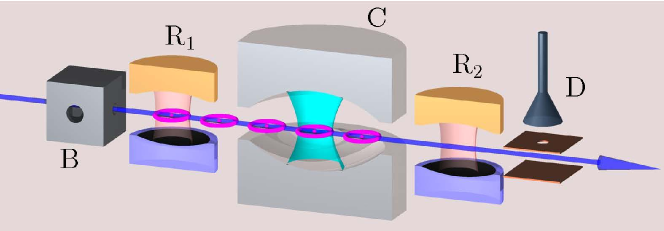
Figure 1: Scheme of the LBK experiment where photons are observed via probe atoms. The photons in blue are trapped between the two mirrors of the cavity $C$. They are probed by two-level atoms (the small pink torus) flying out the preparation box $B$, passing through the cavity $C$ and measured in $D$. Each atom is manipulated before and after $C$ in Ramsey cavities $R_{1}$ and $R_{2}$, respectively. It is finally detected in $D$ either in ground state $|g\rangle$ or in excited state $|e\rangle$.

2.1 The ideal Markov model

The LKB photon box of figure 1, a bi-partite system with the photons as first sub-system and the probe atom as second sub-system, illustrates in an almost perfect and fundamental way the three quantum features listed in the introduction section. This system is a discrete time system with sampling period $\tau$ around $80\leavevmode\nobreak\ \mu s$, the time interval between probe atoms. Step $k\in{\mathbb{N}}$ corresponds to time $t=k\tau$. At $t=k\tau$, the photons are assumed to be described by the wave function $|\psi\rangle_{k}$ of an harmonic oscillator (see appendix A). At $t=k\tau$, the probe atom number $k$, modeled as a qubit (see appendix B), gets outside the box $B$ in ground state $|g\rangle$. Between $t\in[k\tau,(k+1)\tau[$, the wave function $|\Psi\rangle$ of this composite system, photons/atom number $k$, is governed by a Schrödinger evolution

$$\frac{d}{dt}|\Psi\rangle=-\frac{i}{\hbar}\boldsymbol{H}|\Psi\rangle$$

with starting condition $|\Psi\rangle_{k\tau}=|\psi\rangle_{k}\otimes|g\rangle$ and where $\boldsymbol{H}$ is the photons/atom Hamiltonian depending possibly on $t$. Appendix C presents typical Hamiltonians in the resonant and dispersive cases. We have thus a propagator between $t=k\tau$ and $t=(k+1)\tau^{-}$, $U_{(k\tau,(k+1)\tau^{-})}$, from which we get $|\Psi\rangle$ at time $t=(k+1)\tau^{-}$, just before detector $D$ where the energy of the atom is measured via $\boldsymbol{O}=\boldsymbol{I}_{S}\otimes\boldsymbol{\sigma_{\!z}}$. The following relation,

$$|\Psi\rangle_{(k+1)\tau^{-}}=U_{(k\tau,(k+1)\tau^{-})}|\psi\rangle_{k}\otimes|g\rangle\triangleq\boldsymbol{M}_{g}|\psi\rangle_{k}\otimes|g\rangle+\boldsymbol{M}_{e}|\psi\rangle_{k}\otimes|e\rangle,$$

valid for any $|\psi\rangle_{k}$, defines the measurement operators $\boldsymbol{M}_{g}$ and $\boldsymbol{M}_{e}$ on the Hilbert space of the photons $\mathcal{H}_{S}$. Since, for all $|\psi\rangle_{k}$, $|\Psi\rangle_{(k+1)\tau^{-}}$ is of length $1$, we have necessarily $\boldsymbol{M}_{g}^{\dagger}\boldsymbol{M}_{g}+\boldsymbol{M}_{e}^{\dagger}\boldsymbol{M}_{e}=\boldsymbol{I}_{S}$. At time $t=(k+1)\tau^{-}$, we measure $\boldsymbol{O}=\lambda_{e}\boldsymbol{I}_{S}\otimes|e\rangle\langle e|+\lambda_{g}\boldsymbol{I}_{S}\otimes|g\rangle\langle g|$ with two highly degenerate eigenvalues $\lambda_{e}=1$, $\lambda_{g}=-1$ of eigenspaces $\mathcal{H}_{S}\otimes|e\rangle$ and $\mathcal{H}_{S}\otimes|g\rangle$, respectively. According to the measurement quantum rules, we can get only two outcomes $\mu$, either $\mu=g$ or $\mu=e$. With outcome $\mu$, just after the measurement, at time $(k+1)\tau$ the quantum state $|\Psi\rangle$ is changed to

$$|\Psi\rangle_{(k+1)\tau^{-}}\mapsto|\Psi\rangle_{(k+1)\tau}=\frac{\boldsymbol{M}_{\mu}|\psi\rangle_{k}}{\sqrt{\langle\psi_{k}|\boldsymbol{M}_{\mu}^{\dagger}\boldsymbol{M}_{\mu}|\psi_{k}\rangle}}\otimes|\mu\rangle.$$

Moreover the probability to get $\mu$ is $\langle\psi_{k}|\boldsymbol{M}_{\mu}^{\dagger}\boldsymbol{M}_{\mu}|\psi_{k}\rangle$. Since $|\Psi\rangle_{(k+1)\tau}$ is now a simple tensor product (separate state), we can forget the atom number $k$ and summarize the evolution of the photon wave function between $t=k\tau$ and $t=(k+1)\tau$ by the following Markov process

$$|\psi\rangle_{k+1}=\left\{\begin{array}[]{ll}\frac{\boldsymbol{M}_{g}|\psi\rangle_{k}}{\sqrt{\langle\psi_{k}|\boldsymbol{M}_{g}^{\dagger}\boldsymbol{M}_{g}|\psi_{k}\rangle}},&\hbox{with probability $\langle\psi_{k}|\boldsymbol{M}_{g}^{\dagger}\boldsymbol{M}_{g}|\psi_{k}\rangle$;}\\ \frac{\boldsymbol{M}_{e}|\psi\rangle_{k}}{\sqrt{\langle\psi_{k}|\boldsymbol{M}_{e}^{\dagger}\boldsymbol{M}_{g}|\psi_{k}\rangle}},&\hbox{with probability $\langle\psi_{k}|\boldsymbol{M}_{e}^{\dagger}\boldsymbol{M}_{e}|\psi_{k}\rangle$.}\end{array}\right.$$

More generally, for an arbitrary quantum state $\rho_{k}$ of the photons at step $k$, we have

$$\rho_{k+1}=\left\{\begin{array}[]{ll}\frac{\boldsymbol{M}_{g}\rho_{k}\boldsymbol{M}_{g}^{\dagger}}{\operatorname{Tr}\left(\boldsymbol{M}_{g}\rho_{k}\boldsymbol{M}_{g}^{\dagger}\right)},&\hbox{with probability $p_{g}(\rho_{k})=\operatorname{Tr}\left(\boldsymbol{M}_{g}\rho_{k}\boldsymbol{M}_{g}^{\dagger}\right)$;}\\ \frac{\boldsymbol{M}_{e}\rho_{k}\boldsymbol{M}_{e}^{\dagger}}{\operatorname{Tr}\left(\boldsymbol{M}_{e}\rho_{k}\boldsymbol{M}_{e}^{\dagger}\right)},&\hbox{with probability $p_{e}(\rho_{k})=\operatorname{Tr}\left(\boldsymbol{M}_{e}\rho_{k}\boldsymbol{M}_{e}^{\dagger}\right)$.}\end{array}\right.$$ (3)

The measurement operators $\boldsymbol{M}_{g}$ and $\boldsymbol{M}_{e}$ are implicitly defined by the Schrödinger propagator between $k\tau$ and $(k+1)\tau$. They always satisfy $\boldsymbol{M}_{g}^{\dagger}\boldsymbol{M}_{g}+\boldsymbol{M}_{e}^{\dagger}\boldsymbol{M}_{e}=\boldsymbol{I}_{S}$.

2.2 Quantum Non Demolition (QND) measurement

For a well tuned composite evolution $U_{(k\tau,(k+1)\tau^{-})}$ (see [33]) with a dispersive interaction, one get the following measurement operators, functions of the photon-number operator ${\boldsymbol{N}}$,

$$\boldsymbol{M}_{g}=\cos\left(\tfrac{\phi_{0}{\boldsymbol{N}}+\phi_{R}}{2}\right),\quad\boldsymbol{M}_{e}=\sin\left(\tfrac{\phi_{0}{\boldsymbol{N}}+\phi_{R}}{2}\right)$$ (4)

where $\phi_{0}$ and $\phi_{R}$ are tunable real parameters. The Markov process (3) admits then a lot of interesting properties characterizing QND measurement.

• For any function $g:{\mathbb{R}}\mapsto{\mathbb{R}}$, $V_{g}(\rho)=\operatorname{Tr}\left(g({\boldsymbol{N}})\rho\right)$ is a martingale:

  $$\mathbb{E}\left(V_{g}(\rho_{k+1})\leavevmode\nobreak\ /\leavevmode\nobreak\ \rho_{k}\right)=V_{g}(\rho_{k})$$

  where $\mathbb{E}\left(x\leavevmode\nobreak\ /\leavevmode\nobreak\ y\right)$ stands for conditional expectation of $x$ knowing $y$. This results from elementary properties of the trace and from the commutation of $\boldsymbol{M}_{g}$ and $\boldsymbol{M}_{e}$ with ${\boldsymbol{N}}$.

• For any integer $\bar{n}$, the photon-number state $|\bar{n}\rangle\langle\bar{n}|$ ($\bar{n}\in{\mathbb{N}}$) is a steady-state: any realization of (3) starting from $\rho_{0}=|\bar{n}\rangle\langle\bar{n}|$ is constant: $\forall k\geq 0$, $\rho_{k}\equiv|\bar{n}\rangle\langle\bar{n}|$.

• When $(\phi_{R},\phi_{0},\pi)$ are $\mathbb{Q}$-independent, there is no other steady state than these photon-number states. Moreover, for any initial density operator $\rho_{0}$ with a finite photon-number support ($\rho_{0}|m\rangle=0$ for $m$ large enough), the probability that $\rho_{k}$ converges towards the steady state $|\bar{n}\rangle\langle\bar{n}|$ is $\operatorname{Tr}\left(|\bar{n}\rangle\langle\bar{n}|\rho_{0}\right)=\langle\bar{n}|\rho_{0}|\bar{n}\rangle$. Since $\operatorname{Tr}\left(\rho_{0}\right)=1=\sum_{\bar{n}\in{\mathbb{N}}}\langle\bar{n}|\rho_{0}|\bar{n}\rangle$, the Markov process (3) converges almost surely towards a photon-number state, whatever its initial state $\rho_{0}$ is.

The proof of this convergence result is essentially based on a Lyapunov function, a super-martingale, $V(\rho)=-\sum_{n\in{\mathbb{N}}}\langle n\left|\rho\right|n\rangle^{2}$. Simple computations yield

$$\mathbb{E}\left(V(\rho_{k+1})\leavevmode\nobreak\ /\leavevmode\nobreak\ \rho_{k}\right)=V(\rho_{k})-Q(\rho_{k})$$

where $Q(\rho)\geq 0$ is given by the following formula

$$Q(\rho)=\tfrac{\left(\sum_{n^{\prime}}\cos^{2}\left(\tfrac{\phi_{0}n^{\prime}+\phi_{R}}{2}\right)\langle n^{\prime}|\rho|n^{\prime}\rangle\right)\left(\sum_{n^{\prime}}\sin^{2}\left(\tfrac{\phi_{0}n^{\prime}+\phi_{R}}{2}\right)\langle n^{\prime}|\rho|n^{\prime}\rangle\right)}{4}\\ \left(\sum_{n\in{\mathbb{N}}}\left(\tfrac{\cos^{2}\left(\tfrac{\phi_{0}n+\phi_{R}}{2}\right)\langle n|\rho|n\rangle}{\sum_{n^{\prime}}\cos^{2}\left(\tfrac{\phi_{0}n^{\prime}+\phi_{R}}{2}\right)\langle n^{\prime}|\rho|n^{\prime}\rangle}-\tfrac{\sin^{2}\left(\tfrac{\phi_{0}n+\phi_{R}}{2}\right)\langle n|\rho|n\rangle}{\sum_{n^{\prime}}\sin^{2}\left(\tfrac{\phi_{0}n^{\prime}+\phi_{R}}{2}\right)\langle n^{\prime}|\rho|n^{\prime}\rangle}\right)^{2}\right).$$

Since $(\phi_{0},\phi_{R},\pi)$ are $\mathbb{Q}$-independent, $Q(\rho)=0$ implies that, for some $\bar{n}\in{\mathbb{N}}$, $\rho=|\bar{n}\rangle\langle\bar{n}|$. One concludes then with usual probability and compactness arguments [39], despite the fact that the underlying Hilbert space is of infinite dimension. Other and also more precise results can be found in [9].

2.3 Stabilization of photon-number states by feedback

Take $\bar{n}\in{\mathbb{N}}$. With measurement operators (4), the Markov process (3) admits $\bar{\rho}=|\bar{n}\rangle\langle\bar{n}|$ as steady state. We describe here the measurement-based feedback (quantum-state feedback) implemented experimentally in [57] and that stabilizes $\bar{\rho}$. Here the scalar classical control input $u$ consists in applying, just after the atom measurement in $D$, a coherent displacement of tunable amplitude $u$. This yields the following control Markov process

$$\rho_{k+1}=\left\{\begin{aligned} &\frac{\boldsymbol{D}_{u_{k}}\boldsymbol{M}_{g}\rho_{k}\boldsymbol{M}_{g}^{\dagger}\boldsymbol{D}_{u_{k}}^{\dagger}}{\operatorname{Tr}\left(\boldsymbol{M}_{g}\rho_{k}\boldsymbol{M}_{g}^{\dagger}\right)}\quad\text{$y_{k}=g$ with probability }p_{g,k}=\operatorname{Tr}\left(\boldsymbol{M}_{g}\rho_{k}\boldsymbol{M}_{g}^{\dagger}\right)&\\ &\frac{\boldsymbol{D}_{u_{k}}\boldsymbol{M}_{e}\rho_{k}\boldsymbol{M}_{e}^{\dagger}\boldsymbol{D}_{u_{k}}^{\dagger}}{\operatorname{Tr}\left(\boldsymbol{M}_{e}\rho_{k}\boldsymbol{M}_{e}^{\dagger}\right)}\quad\text{$y_{k}=e$ with probability }p_{e,k}=\operatorname{Tr}\left(\boldsymbol{M}_{e}\rho_{k}\boldsymbol{M}_{e}^{\dagger}\right)&\end{aligned}\right.$$ (5)

where $u_{k}\in{\mathbb{R}}$ is the control at step $k$, $\boldsymbol{D}_{u}=e^{u\boldsymbol{a}^{\dagger}-u\boldsymbol{a}}$ is the displacement of amplitude $u$ (see appendix A) and $y_{k}$ is the measurement outcome at step $k$.

The stabilization of $\bar{\rho}$ is based on a state-feedback function $f$, $u=f(\rho)$, such that almost all closed-loop trajectories of (5) with $u_{k}=f(\rho_{k})$ converge towards $\bar{\rho}$ for any initial condition $\rho_{0}$. The construction of $f$ exploits the open-loop martingales $\operatorname{Tr}\left(g({\boldsymbol{N}})\rho\right)$ to construct the following strict control Lyapunov function:

$$V_{\epsilon}(\rho)=\sum_{n}\left(-\epsilon\langle n\left|\rho\right|n\rangle^{2}+\sigma_{n}\langle n|\rho|n\rangle\right)$$

where $\epsilon>0$ is small enough and

$$\sigma_{n}=\left\{\begin{array}[]{ll}\tfrac{1}{4}+\sum_{\nu=1}^{\bar{n}}\tfrac{1}{\nu}-\tfrac{1}{\nu^{2}},&\hbox{if }n=0;\\ \sum_{\nu=n+1}^{\bar{n}}\tfrac{1}{\nu}-\tfrac{1}{\nu^{2}},&\hbox{if }n\in[1,\bar{n}-1];\\ 0,&\hbox{if }n=\bar{n};\\ \sum_{\nu=\bar{n}+1}^{n}\tfrac{1}{\nu}+\tfrac{1}{\nu^{2}},&\hbox{if }n\in[\bar{n}+1,+\infty].\end{array}\right.$$

The weight $\sigma_{n}$ are all non negative, $n\mapsto\sigma_{n}$ is strictly decreasing (resp. increasing) for $n\leq\bar{n}$ (resp. $n\geq\bar{n}$) and minimum for $n=\bar{n}$. The feedback law $u=f(\rho)$ is obtained by choosing $u$ such that the expectation value of $V_{\epsilon}(\rho_{k+1})$, knowing $\rho_{k}=\rho$ and $u_{k}=u$, is as small as possible:

$$u=f(\rho)=:\underset{\upsilon\in[-\bar{u},\bar{u}]}{\text{Argmin}}\quad V_{\epsilon}\Big{(}\boldsymbol{D}_{\upsilon}\left(\boldsymbol{M}_{g}\rho\boldsymbol{M}_{g}^{\dagger}+\boldsymbol{M}_{e}\rho\boldsymbol{M}_{e}^{\dagger}\right)\boldsymbol{D}_{\upsilon}^{\dagger}\Big{)}$$

where $\bar{u}>0$ is some prescribed bound on $|u|$. Such a feedback law achieves global stabilization since, in closed-loop, the Lyapunov function is strict:

$$\forall\rho\neq|\bar{n}\rangle\langle\bar{n}|,\quad V_{\epsilon}\Big{(}\boldsymbol{D}_{f(\rho)}\left(\boldsymbol{M}_{g}\rho\boldsymbol{M}_{g}^{\dagger}+\boldsymbol{M}_{e}\rho\boldsymbol{M}_{e}^{\dagger}\right)\boldsymbol{D}_{f(\rho)}^{\dagger}\Big{)}<V_{\epsilon}\Big{(}\rho\Big{)}.$$

Formal convergence proofs can be found in [3] for any finite dimensional approximations resulting from a truncation to a finite number of photons and in [60] for the infinite dimension.

2.4 A more realistic Markov model with detection errors

The experimental implementation of the above feedback law [57] has to cope with several sources of imperfections. We focus here on measurement errors and show how the Markov process has to be changed to take into account these errors. Assume that we know the detection error rates characterized by $\mathbb{P}(y=e/\mu=g)=\eta_{g}\in[0,1]$ (resp. $\mathbb{P}(y=g/\mu=e)=\eta_{e}\in[0,1]$) the probability of erroneous assignation to $e$ (resp. $g$) when the atom collapses in $g$ (resp. $e$). Without error, the quantum state $\rho_{k}$ obeys to (3). A direct application of Bayes law provides the expectation of $\rho_{k+1}$, knowing $\rho_{k}$ and the effective detector signal $y_{k}$, possibly corrupted by a detection error. When $y_{k}=g$, this expectation value is given by $\frac{(1-\eta_{g})\boldsymbol{M}_{g}\rho_{k}\boldsymbol{M}_{g}^{\dagger}+\eta_{e}\boldsymbol{M}_{e}\rho_{k}\boldsymbol{M}_{e}^{\dagger}}{\operatorname{Tr}\left((1-\eta_{g})\boldsymbol{M}_{g}\rho_{k}\boldsymbol{M}_{g}^{\dagger}+\eta_{e}\boldsymbol{M}_{e}\rho_{k}\boldsymbol{M}_{e}^{\dagger}\right)}$ and, when $y_{k}=e$, by $\frac{\eta_{g}\boldsymbol{M}_{g}\rho_{k}\boldsymbol{M}_{g}^{\dagger}+(1-\eta_{e})\boldsymbol{M}_{e}\rho_{k}\boldsymbol{M}_{e}^{\dagger}}{\operatorname{Tr}\left(\eta_{g}\boldsymbol{M}_{g}\rho_{k}\boldsymbol{M}_{g}^{\dagger}+(1-\eta_{e})\boldsymbol{M}_{e}\rho_{k}\boldsymbol{M}_{e}^{\dagger}\right)}.$ Moreover the probability to get $y_{k}=g$ is $\operatorname{Tr}\left((1-\eta_{g})\boldsymbol{M}_{g}\rho_{k}\boldsymbol{M}_{g}^{\dagger}+\eta_{e}\boldsymbol{M}_{e}\rho_{k}\boldsymbol{M}_{e}^{\dagger}\right)$ and to get $y_{k}=e$ is $\operatorname{Tr}\left(\eta_{g}\boldsymbol{M}_{g}\rho\boldsymbol{M}_{g}^{\dagger}+(1-\eta_{e})\boldsymbol{M}_{e}\rho\boldsymbol{M}_{e}^{\dagger}\right)$. This means that the Markov process (3) must be changed to

$$\rho_{k+1}=\left\{\begin{array}[]{ll}\frac{(1-\eta_{g})\boldsymbol{M}_{g}\rho_{k}\boldsymbol{M}_{g}^{\dagger}+\eta_{e}\boldsymbol{M}_{e}\rho_{k}\boldsymbol{M}_{e}^{\dagger}}{\operatorname{Tr}\left((1-\eta_{g})\boldsymbol{M}_{g}\rho_{k}\boldsymbol{M}_{g}^{\dagger}+\eta_{e}\boldsymbol{M}_{e}\rho_{k}\boldsymbol{M}_{e}^{\dagger}\right)}&\hbox{ when $y_{k}=g$,}\\[10.00002pt] \frac{\eta_{g}\boldsymbol{M}_{g}\rho_{k}\boldsymbol{M}_{g}^{\dagger}+(1-\eta_{e})\boldsymbol{M}_{e}\rho_{k}\boldsymbol{M}_{e}^{\dagger}}{\operatorname{Tr}\left(\eta_{g}\boldsymbol{M}_{g}\rho_{k}\boldsymbol{M}_{g}^{\dagger}+(1-\eta_{e})\boldsymbol{M}_{e}\rho_{k}\boldsymbol{M}_{e}^{\dagger}\right)}&\hbox{ when $y_{k}=e$,}\end{array}\right.$$ (6)

with $\operatorname{Tr}\left((1-\eta_{g})\boldsymbol{M}_{g}\rho_{k}\boldsymbol{M}_{g}^{\dagger}+\eta_{e}\boldsymbol{M}_{e}\rho_{k}\boldsymbol{M}_{e}^{\dagger}\right)$ and $\operatorname{Tr}\left(\eta_{g}\boldsymbol{M}_{g}\rho_{k}\boldsymbol{M}_{g}^{\dagger}+(1-\eta_{e})\boldsymbol{M}_{e}\rho_{k}\boldsymbol{M}_{e}^{\dagger}\right)$ being the probabilities to detect $y_{k}=g$ and $e$, respectively. The quantum state $\rho_{k}$ is thus a conditional state: it is the expectation value of the projector associated to the photon wave function at step $k$, knowing its value at step $k=0$ and the detection outcomes $(y_{0},\ldots,y_{k-1})$.

All other experimental imperfections including decoherence can be treated in the same way (see, e.g., [26, 59]) and yield to a quantum state governed by a Markov process with a similar structure. In fact all usual models of open quantum systems admit the same structure, either in discrete-time (see section 3) or in continuous-time (see section 4).

2.5 The real-time stabilization algorithm

Let us give more details on the real-time implementation used in [57] of this quantum-state feedback. The sampling period $\tau$ is around $80\leavevmode\nobreak\ \mu s$. The controller set-point is an integer $\bar{n}$ labelling the steady-state $\bar{\rho}=|\bar{n}\rangle\langle\bar{n}|$ to be stabilized. At time step $k$, the real-time computer

1. reads $y_{k}$ the measurement outcome for probe atom $k$;

2. updates the quantum state from previous step value $\rho_{k-1}$ to $\rho_{k}$ using $y_{k}$ and a Markov model slightly more complicated but of same structure as (6); this update corresponds to a quantum filter (see subsection 3.3).

3. computes $u_{k}$ as $f(\rho_{k})$ (state feedback) where $f$ results from minimizing the expectation of the control Lyapunov function $V_{\epsilon}(\rho)$ at step $k+1$, knowing $\rho_{k}$;

4. send via an antenna a micro-wave pulse calibrated to obtain the displacement $\boldsymbol{D}_{u_{k}}$ on the photons.

All the details of this quantum feedback are given in [56]. In particular, the Markov model takes into account several experimental imperfections such as finite life-time of the photons (around $1/10\leavevmode\nobreak\ s$) and a delay of $5$ steps in the feedback loop. Convergence results related to this feedback scheme are given in [3].

2.6 Reservoir engineering stabilization of Schrödinger cats

It is possible to stabilize the photons trapped in cavity $C$ (figure 1) without any such measurement-based feedback, just by well tuned interactions with the probe atoms and without measuring them in $D$. Such kind of stabilization, known as reservoir engineering [51], can be seen as a generalization of optical pumping techniques [37]. Such stabilization methods are illustrative of coherent (or autonomous) feedback where the controller is an open quantum system. In [54], a realistic implementation of such passive stabilization method is proposed. It stabilizes a coherent superposition of classical photon-states with opposite phases, a Schrödinger phase-cats with wave functions of the form $(|\alpha\rangle+i|\text{-}\alpha\rangle)/\sqrt{2}$, where $|\alpha\rangle$ is the coherent state of amplitude $\alpha\in{\mathbb{R}}$. We explain here the convergence analysis of such passive stabilization using the notations and operator definitions given in appendix A.

The atom entering the cavity $C$ is prepared through $R_{1}$ in a partially excited state $\cos(u/2)|g\rangle+\sin(u/2)|e\rangle$ with $u\in[0,\pi/2[$ (south hemisphere of the Bloch sphere). Its interaction with the photons is first dispersive with positive detuning during its entrance, then resonant in the cavity middle and finally dispersive with negative detuning when leaving the cavity. The resulting measurement operators $\boldsymbol{M}_{g}$ and $\boldsymbol{M}_{e}$ appearing in (3) admit then the following form (see [55] for detailed derivations):

$$\boldsymbol{M}_{g}=e^{-i\widetilde{h}({\boldsymbol{N}})}\boldsymbol{\widetilde{M}}_{g}e^{i\widetilde{h}({\boldsymbol{N}})},\quad\boldsymbol{M}_{e}=e^{-i\widetilde{h}({\boldsymbol{N}})}\boldsymbol{\widetilde{M}}_{e}e^{i\widetilde{h}({\boldsymbol{N}})}$$

with $n\mapsto\widetilde{h}(n)$ a real function, with $\boldsymbol{I}$ standing for $\boldsymbol{I}_{S}$, with

$$\boldsymbol{\widetilde{M}}_{g} =\cos(\tfrac{u}{2})\cos\left(\tfrac{\theta({\boldsymbol{N}})}{2}\right)+\epsilon\sin(\tfrac{u}{2})\frac{\sin\left(\tfrac{\theta({\boldsymbol{N}})}{2}\right)}{\sqrt{{\boldsymbol{N}}}}\,\boldsymbol{a}^{\dagger}$$

$$\boldsymbol{\widetilde{M}}_{e} =\sin(\tfrac{u}{2})\cos\left(\tfrac{\theta({{\boldsymbol{N}}+\boldsymbol{I}})}{2}\right)-\epsilon\cos(\tfrac{u}{2})\,\boldsymbol{a}\frac{\sin\left(\tfrac{\theta({\boldsymbol{N}})}{2}\right)}{\sqrt{{\boldsymbol{N}}}}$$

and with $n\mapsto\theta(n)$ a real function such that $\theta(0)=0$, $\forall n>0$, $\theta(n)\in]0,\pi[$ and $\lim_{n\mapsto+\infty}\theta(n)=\pi/2$.

Since we do not measure the atoms, the photon state $\rho_{k+1}$ at step $k+1$ is given by the following recurrence from the state $\rho_{k}$ at step $k$:

$$\rho_{k+1}=\boldsymbol{K}(\rho_{k})\triangleq\boldsymbol{M}_{g}\rho_{k}\boldsymbol{M}_{g}^{\dagger}+\boldsymbol{M}_{e}\rho_{k}\boldsymbol{M}_{e}^{\dagger}.$$

Consider the change of frame associated to the unitary transformation $e^{-i\widetilde{h}({\boldsymbol{N}})}$: $\rho=e^{-i\widetilde{h}({\boldsymbol{N}})}\widetilde{\rho}e^{i\widetilde{h}({\boldsymbol{N}})}.$ Then we have $\widetilde{\rho}_{k+1}=\boldsymbol{\widetilde{K}}(\widetilde{\rho}_{k})\triangleq\boldsymbol{\widetilde{M}}_{g}\widetilde{\rho}_{k}(\boldsymbol{\widetilde{M}}_{g})^{\dagger}+\boldsymbol{\widetilde{M}}_{e}\widetilde{\rho}_{k}(\boldsymbol{\widetilde{M}}_{e})^{\dagger}.$ It is proved in [40] that, since $|u|\leq\pi/2$, exists a unique common eigen-state $|\widetilde{\psi}\rangle\in\mathcal{H}_{S}$ of $\boldsymbol{\widetilde{M}}_{g}$ and $\boldsymbol{\widetilde{M}}_{e}$. Thus $\widetilde{\rho}_{\infty}=|\widetilde{\psi}\rangle\langle\widetilde{\psi}|$ is a fixed point of $\boldsymbol{\widetilde{K}}$. It is also proved in [40] that the $\widetilde{\rho}_{k}$’s converge to $\widetilde{\rho}_{\infty}$ when the function $\theta$ is strictly increasing. Since the underlying Hilbert space $\mathcal{H}_{S}$ is of infinite dimension, it is important to precise the type of convergence. For any initial condition $\widetilde{\rho}_{0}$ such that $\operatorname{Tr}\left({\boldsymbol{N}}\widetilde{\rho}_{0}\right)<+\infty$, then $\lim_{k\mapsto+\infty}\operatorname{Tr}\left((\widetilde{\rho}_{k}-\widetilde{\rho}_{\infty})^{2}\right)=0$ (Frobenius norm on Hilbert-Schmidt operators). Since $\operatorname{Tr}\left({\boldsymbol{N}}\rho\right)\equiv\operatorname{Tr}\left({\boldsymbol{N}}\widetilde{\rho}\right)$, we have the convergence of $\rho_{k}$ towards $\rho_{\infty}=e^{-i\widetilde{h}({\boldsymbol{N}})}\widetilde{\rho}_{\infty}e^{i\widetilde{h}({\boldsymbol{N}})}$ as soon as the initial energy $\operatorname{Tr}\left({\boldsymbol{N}}\rho_{0}\right)$ is finite: $\lim_{k\mapsto+\infty}\operatorname{Tr}\left(\left((\rho_{k}-\rho_{\infty}\right)^{2}\right)=0$. When $\theta$ is not strictly increasing, we conjecture that such convergence towards $\rho_{\infty}$ still holds true.

For well chosen experimental parameters [55], $\widetilde{\rho}_{\infty}$ is close to a coherent state $|\alpha_{\infty}\rangle\langle\alpha_{\infty}|$ for some $\alpha_{\infty}\in{\mathbb{R}}$ and $\widetilde{h}({\boldsymbol{N}})\approx\pi{\boldsymbol{N}}^{2}/2$ . Since

$$e^{-i\frac{\pi}{2}{\boldsymbol{N}}^{2}}|\alpha_{\infty}\rangle=\frac{e^{-i\pi/4}}{\sqrt{2}}\big{(}|\alpha_{\infty}\rangle+i|\text{-}\alpha_{\infty}\rangle\big{)},$$

we have under realistic conditions $\lim_{k\mapsto+\infty}\rho_{k}\approx\tfrac{1}{2}\Big{(}|\alpha_{\infty}\rangle+i|\text{-}\alpha_{\infty}\rangle\Big{)}\Big{(}\langle\alpha_{\infty}|-i\langle\text{-}\alpha_{\infty}|\Big{)}$, a coherent superposition of the classical states $|\alpha_{\infty}\rangle$ and $|\text{-}\alpha_{\infty}\rangle$ of same amplitude but of opposite phases, i.e. a Schrödinger phase-cat. Figure 2 displays numerical computations of the Wigner function of $\rho_{\infty}$ obtained with realistic parameters.

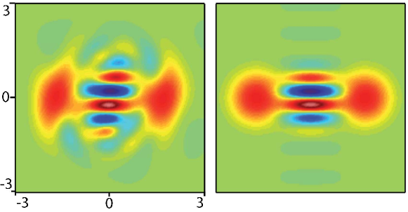
Figure 2: Left: Wigner function of $\rho_{\infty}$ stabilized by reservoir engineering in [55]. Right: Wigner function of a prefect Schrödinger phase-cat, $\tfrac{1}{2}\Big{(}|\alpha_{\infty}\rangle+i|\text{-}\alpha_{\infty}\rangle\Big{)}\Big{(}\langle\alpha_{\infty}|+i\langle\text{-}\alpha_{\infty}|\Big{)}$, with an average number of photons identical to $\rho_{\infty}$ ($\alpha_{\infty}=\sqrt{\operatorname{Tr}\left({\boldsymbol{N}}\rho_{\infty}\right)}$). The color map is identical to figure 3.

3 Discrete-time systems

The theory of open quantum systems starts with the contributions of Davies [25]. The goal of this section is first to present in an elementary way the general structure of the Markov models describing such systems. Some related stabilization problems are also addressed. Throughout this section, $\mathcal{H}$ is an Hilbert space; for each time-step $k\in{\mathbb{N}}$, $\rho_{k}$ denotes the density operator describing the state of the quantum Markov process; for all $k$, $\rho_{k}$ is an Hilbert-Schmidt operator on $\mathcal{H}$, Hermitian and of trace one; the set of continuous operators on $\mathcal{H}$ is denoted by $\mathcal{L}(\mathcal{H})$; expectation values are denoted by the symbol $\mathbb{E}\left(\leavevmode\nobreak\ \right)$.

3.1 Markov models

Take a positive integer $m$ and consider a finite set $(\boldsymbol{M}_{\mu})_{\mu\in\{1,\ldots,m\}}$ of operators on $\mathcal{H}$ such that

$$\boldsymbol{I}=\sum_{\mu=1}^{m}\boldsymbol{M}_{\mu}^{\dagger}\boldsymbol{M}_{\mu}$$ (7)

where $\boldsymbol{I}$ is the identity operator. Then each $\boldsymbol{M}_{\mu}\in\mathcal{L}(\mathcal{H})$. Take another positive integer $m^{\prime}$ and consider a left stochastic $m^{\prime}\times m$-matrix $(\eta_{\mu^{\prime}\mu})$: its entries are non-negative and $\forall\mu\in\{1,\ldots,m\}$, $\sum_{\mu^{\prime}=1}^{m^{\prime}}\eta_{\mu^{\prime}\mu}=1$. Consider the Markov process of state $\rho$ and output $y\in\{1,\ldots,m^{\prime}\}$ (measurement outcome) defined via the transition rule

$$\rho_{k+1}=\frac{\sum_{\mu}\eta_{\mu^{\prime}\mu}\boldsymbol{M}_{\mu}\rho_{k}\boldsymbol{M}_{\mu}^{\dagger}}{\operatorname{Tr}\left(\sum_{\mu}\eta_{\mu^{\prime}\mu}\boldsymbol{M}_{\mu}\rho_{k}\boldsymbol{M}_{\mu}^{\dagger}\right)},\quad y_{k}=\mu^{\prime}\text{ with probability }\mathbb{P}_{\mu^{\prime}}(\rho_{k})$$ (8)

where $\mathbb{P}_{\mu^{\prime}}(\rho)=\operatorname{Tr}\left(\sum_{\mu}\eta_{\mu^{\prime}\mu}\boldsymbol{M}_{\mu}\rho\boldsymbol{M}_{\mu}^{\dagger}\right)$.

3.2 Kraus and unital maps

The Kraus map $\boldsymbol{K}$ corresponds to the master equation of (8). It is given by the expectation value of $\rho_{k+1}$ knowing $\rho_{k}$:

$$\boldsymbol{K}(\rho)\triangleq\sum_{\mu}\boldsymbol{M}_{\mu}\rho\boldsymbol{M}_{\mu}^{\dagger}=\mathbb{E}\left(\rho_{k+1}\leavevmode\nobreak\ /\leavevmode\nobreak\ \rho_{k}=\rho\right).$$ (9)

In quantum information [48] such Kraus maps describe quantum channels. They admit many interesting properties. In particular, they are contractions for many metrics (see [50] for the characterization, in finite dimension, of metrics for which any Kraus map is a contraction). We just recall below two such metrics. For any density operators $\rho$ and $\sigma$ we have

$$D(\boldsymbol{K}(\rho),\boldsymbol{K}(\sigma))\leq D(\rho,\sigma)\text{ and }F(\boldsymbol{K}(\rho),\boldsymbol{K}(\sigma))\geq F(\rho,\sigma)$$ (10)

where the trace distance $D$ and fidelity $F$ are given by

$$D(\rho,\sigma)\triangleq\operatorname{Tr}\left(|\rho-\sigma|\right)\text{ and }F(\rho,\sigma)\triangleq\operatorname{Tr}^{2}\left(\sqrt{\sqrt{\rho}\sigma\sqrt{\rho}}\right).$$ (11)

Fidelity is between $0$ and $1$: $F(\rho,\sigma)=1$ if and only if, $\rho=\sigma$. Moreover $F(\rho,\sigma)=F(\sigma,\rho)$. If $\sigma=|\psi\rangle\langle\psi|$ is a pure state ($|\psi\rangle$ element of $\mathcal{H}$ of length one), $F(\rho,\sigma)$ coincides with the Frobenius product: $F(\rho,|\psi\rangle\langle\psi|)\equiv\operatorname{Tr}\left(\rho|\psi\rangle\langle\psi|\right)=\langle\psi|\rho|\psi\rangle.$ Kraus maps provide the evolution of open quantum systems from an initial state $\rho_{0}$ without information coming from the measurements (see [33, chapter 4: the environment is watching]):

$$\rho_{k+1}=\boldsymbol{K}(\rho_{k})\text{ for }k=0,1,\ldots,.$$

This corresponds to the ”Schrödinger description” of the dynamics.

The ”Heisenberg description” is given by the dual map $\boldsymbol{K}^{*}$. It is characterized by $\operatorname{Tr}\left(A\boldsymbol{K}(\rho)\right)=\operatorname{Tr}\left(\boldsymbol{K}^{*}(A)\rho\right)$ and defined for any operator $A$ on $\mathcal{H}$ by

$$\boldsymbol{K}^{*}(A)=\sum_{\mu}\boldsymbol{M}_{\mu}^{\dagger}A\boldsymbol{M}_{\mu}.$$

Technical conditions on $A$ are required when $\mathcal{H}$ is of infinite dimension, they are not given here (see, e.g., [25]). The map $\boldsymbol{K}^{*}$ is unital since (7) reads $\boldsymbol{K}^{*}(\boldsymbol{I})=\boldsymbol{I}$. As $\boldsymbol{K}$, the dual map $\boldsymbol{K}^{*}$ admits a lot of interesting properties. It is noticed in [58] that, based on a theorem due of Birkhoff [14], such unital maps are contractions on the cone of non-negative Hermitian operators equipped with the Hilbert’s projective metric. In particular, when $\mathcal{H}$ is of finite dimension, we have, for any Hermitian operator $A$:

$$\lambda_{min}(A)\leq\lambda_{min}(\boldsymbol{K}^{*}(A))\leq\lambda_{max}(\boldsymbol{K}^{*}(A))\leq\lambda_{max}(A)$$

where $\lambda_{min}$ and $\lambda_{max}$ correspond to the smallest and largest eigenvalues. As shown in [52], such contraction properties based on Hilbert’s projective metric have important implications in quantum information theory.

To emphasize the difference between the ”Schrödinger description” and the ’Heisenberg description” of the dynamics, let us translate convergence issues from the ”Schrödinger description” to the ”Heisenberg one”. Assume, for clarity’s sake, that $\mathcal{H}$ is of finite dimension. Suppose also that $\boldsymbol{K}$ admits the density operator $\bar{\rho}$ as unique fixed point and that, for any initial density operator $\rho_{0}$, the density operator at step $k$, $\rho_{k}$, defined by $k$ iterations of $\boldsymbol{K}$, converges towards $\bar{\rho}$ when $k$ tends to $\infty$. Then $k\mapsto D(\rho_{k},\bar{\rho})$ is decreasing and converges to $0$ whereas $k\mapsto F(\rho_{k},\bar{\rho})$ is increasing and converges to $1$.

The translation of this convergence in the ”Heisenberg description” is the following: for any initial operator $A_{0}$, its $k$ iterates via $\boldsymbol{K}^{*}$, $A_{k}$, converge towards $\operatorname{Tr}\left(A_{0}\bar{\rho}\right)\boldsymbol{I}$. Moreover when $A_{0}$ is Hermitian, $k\mapsto\lambda_{min}(A_{k})$ and $k\mapsto\lambda_{max}(A_{k})$ are respectively increasing and decreasing and both converge to $\operatorname{Tr}\left(A_{0}\bar{\rho}\right)$.

3.3 Quantum filtering

Quantum filtering has its origin in Belavkin’s work [13] on continuous-time open quantum systems (see section 4). The state $\rho_{k}$ of (8) is not directly measured: open quantum systems are governed by hidden-state Markov model. Quantum filtering provides an estimate $\rho^{\text{\tiny est}}_{k}$ of $\rho_{k}$ based on an initial guess $\rho^{\text{\tiny est}}_{0}$ (possibly different from $\rho_{0}$) and the measurement outcomes $y_{l}$ between $0$ and $k-1$:

$$\rho^{\text{\tiny est}}_{l+1}=\frac{\sum_{\mu}\eta_{y_{l}\mu}\boldsymbol{M}_{\mu}\rho^{\text{\tiny est}}_{l}\boldsymbol{M}_{\mu}^{\dagger}}{\operatorname{Tr}\left(\sum_{\mu}\eta_{y_{l}\mu}\boldsymbol{M}_{\mu}\rho^{\text{\tiny est}}_{l}\boldsymbol{M}_{\mu}^{\dagger}\right)},\quad l\in\{0,\ldots,k-1\}.$$ (12)

Thus $(\rho,\rho^{\text{\tiny est}})$ is the state of an extended Markov process governed by the following rule

$$\rho_{k+1}=\frac{\sum_{\mu}\eta_{\mu^{\prime}\mu}\boldsymbol{M}_{\mu}\rho_{k}\boldsymbol{M}_{\mu}^{\dagger}}{\operatorname{Tr}\left(\sum_{\mu}\eta_{\mu^{\prime}\mu}\boldsymbol{M}_{\mu}\rho_{k}\boldsymbol{M}_{\mu}^{\dagger}\right)}\text{ and }\rho^{\text{\tiny est}}_{k+1}=\frac{\sum_{\mu}\eta_{\mu^{\prime}\mu}\boldsymbol{M}_{\mu}\rho^{\text{\tiny est}}_{k}\boldsymbol{M}_{\mu}^{\dagger}}{\operatorname{Tr}\left(\sum_{\mu}\eta_{\mu^{\prime}\mu}\boldsymbol{M}_{\mu}\rho^{\text{\tiny est}}_{k}\boldsymbol{M}_{\mu}^{\dagger}\right)}$$

with transition probability $\mathbb{P}_{\mu^{\prime}}(\rho_{k})=\operatorname{Tr}\left(\sum_{\mu}\eta_{\mu^{\prime}\mu}\boldsymbol{M}_{\mu}\rho_{k}\boldsymbol{M}_{\mu}^{\dagger}\right)$ depending on $\rho_{k}$ and independent of $\rho^{\text{\tiny est}}_{k}$.

When $\mathcal{H}$ is of finite dimension, it is shown in [59] with an inequality proved in [53] that such discrete-time quantum filters are always stable in the following sense: the fidelity between $\rho$ and its estimate $\rho^{\text{\tiny est}}$ is a sub-martingale for any initial condition $\rho_{0}$ and $\rho^{\text{\tiny est}}_{0}$: $\mathbb{E}\left(F(\rho_{k+1},\rho^{\text{\tiny est}}_{k+1})\leavevmode\nobreak\ |\leavevmode\nobreak\ (\rho_{k},\rho^{\text{\tiny est}}_{k})\right)\geq F(\rho_{k},\rho^{\text{\tiny est}}_{k}).$ This result does not guaranty that $\rho^{\text{\tiny est}}_{k}$ converges to $\rho_{k}$ when $k$ tends to infinity. The convergence characterization of $\rho^{\text{\tiny est}}$ towards $\rho$ via checkable conditions on the left stochastic matrix $(\eta_{\mu^{\prime}\mu})$ and on the set of operators $(\boldsymbol{M}_{\mu})$ remains an open problem [61, 62].

3.4 Stabilization via measurement-based feedback

Assume now that the operators $\boldsymbol{M}_{\mu}$ appearing in (8) and satisfying (7), depend also on a control input $u$ belonging to some admissible set $\mathcal{U}$ (typically a discrete set or a compact subset of ${\mathbb{R}}^{p}$ for some positive integer $p$). Then we have the following control Markov model with input $u\in\mathcal{U}$, hidden state $\rho$ and measured output $y\in\{1,\ldots,m^{\prime}\}$:

$$\rho_{k+1}=\frac{\sum_{\mu}\eta_{\mu^{\prime}\mu}\boldsymbol{M}_{\mu}(u_{k})\rho_{k}\boldsymbol{M}_{\mu}^{\dagger}(u_{k})}{\operatorname{Tr}\left(\sum_{\mu}\eta_{\mu^{\prime}\mu}\boldsymbol{M}_{\mu}(u_{k})\rho_{k}\boldsymbol{M}_{\mu}^{\dagger}(u_{k})\right)},\leavevmode\nobreak\ y_{k}=\mu^{\prime}\text{ with probability }\mathbb{P}_{\mu^{\prime}}(\rho_{k},u_{k})$$ (13)

where $\mathbb{P}_{\mu^{\prime}}(\rho,u)=\operatorname{Tr}\left(\sum_{\mu}\eta_{\mu^{\prime}\mu}\boldsymbol{M}_{\mu}(u)\rho\boldsymbol{M}_{\mu}^{\dagger}(u)\right)$. Assume that for some nominal admissible input $\bar{u}\in\mathcal{U}$, this Markov process admits a steady state $\bar{\rho}$. This means that, for any $\mu^{\prime}\in\{1,\ldots,m^{\prime}\}$ we have $\sum_{\mu}\eta_{\mu^{\prime}\mu}\boldsymbol{M}_{\mu}(\bar{u})\bar{\rho}\boldsymbol{M}_{\mu}^{\dagger}(\bar{u})=\mathbb{P}_{\mu^{\prime}}(\bar{\rho},\bar{u})\bar{\rho}.$ The measurement-based feedback stabilization of the steady-state $\bar{\rho}$ is the following problem: for any initial condition $\rho_{0}$, find for any $k\in{\mathbb{N}}$ a control input $u_{k}\in\mathcal{U}$ depending only on $\rho_{0}$ and on the past $y$ values, $(y_{0},\ldots,y_{k-1})$, such that $\rho_{k}$ converges almost surely towards $\bar{\rho}$.

Quantum-state feedback scheme, $u=f(\rho)$, can be used here. They can be based on Lyapunov techniques. Potential candidates of Lyapunov functions $V(\rho)$ could be related to the metrics for which the open-loop Kaus map with $\bar{u}$ is contracting. Specific $V$ depending on the precise structure of the system could be more adapted as for the LKB photon box [3]. Such Lyapunov feedback laws are then given by the minimization versus $u\in\mathcal{U}$ of $\mathbb{E}\left(V(\rho_{k+1})\leavevmode\nobreak\ |\leavevmode\nobreak\ \rho_{k}=\rho,u_{k}=u\right)$.

Assume that we have a stabilizing feedback law $u=f(\rho)$: $\bar{u}=f(\bar{\rho})$ and the trajectories of (13) with $u_{k}=f(\rho_{k})$ converge almost surely towards $\bar{\rho}$. Since $\rho$ is not directly accessible, one has to replace $\rho_{k}$ by its estimate $\rho^{\text{\tiny est}}_{k}$ to obtain $u_{k}$. Experimental implementations of such quantum feedback laws admit necessarily an observer/controller structure governed by a Markov process of state $(\rho,\rho^{\text{\tiny est}})$ with the following transition rule:

$$\begin{split}\rho_{k+1}&=\frac{\sum_{\mu}\eta_{\mu^{\prime}\mu}\boldsymbol{M}_{\mu}(f(\rho^{\text{\tiny est}}_{k}))\rho_{k}\boldsymbol{M}_{\mu}^{\dagger}(f(\rho^{\text{\tiny est}}_{k}))}{\operatorname{Tr}\left(\sum_{\mu}\eta_{\mu^{\prime}\mu}\boldsymbol{M}_{\mu}(f(\rho^{\text{\tiny est}}_{k}))\rho_{k}\boldsymbol{M}_{\mu}^{\dagger}(f(\rho^{\text{\tiny est}}_{k}))\right)}\\ \rho^{\text{\tiny est}}_{k+1}&=\frac{\sum_{\mu}\eta_{\mu^{\prime}\mu}\boldsymbol{M}_{\mu}(f(\rho^{\text{\tiny est}}_{k}))\rho^{\text{\tiny est}}_{k}\boldsymbol{M}_{\mu}^{\dagger}(f(\rho^{\text{\tiny est}}_{k}))}{\operatorname{Tr}\left(\sum_{\mu}\eta_{\mu^{\prime}\mu}\boldsymbol{M}_{\mu}(f(\rho^{\text{\tiny est}}_{k}))\rho^{\text{\tiny est}}_{k}\boldsymbol{M}_{\mu}^{\dagger}(f(\rho^{\text{\tiny est}}_{k}))\right)}\end{split}$$ (14)

with probability $\mathbb{P}_{\mu^{\prime}}(\rho_{k},f(\rho^{\text{\tiny est}}_{k}))=\operatorname{Tr}\left(\sum_{\mu}\eta_{\mu^{\prime}\mu}\boldsymbol{M}_{\mu}(f(\rho^{\text{\tiny est}}_{k}))\rho_{k}\boldsymbol{M}_{\mu}^{\dagger}(f(\rho^{\text{\tiny est}}_{k}))\right)$ depending on $\rho_{k}$ and $\rho^{\text{\tiny est}}_{k}$. In [16] a separation principle is proved with elementary arguments (see also [3]): if $\mathcal{H}$ is of finite dimension, if $\bar{\rho}$ is a pure state ($\bar{\rho}=|\bar{\psi}\rangle\langle\bar{\psi}|$ for some $|\bar{\psi}\rangle$ in $\mathcal{H}$) and if $\operatorname{Ker}(\rho^{\text{\tiny est}}_{0})\subset\operatorname{Ker}(\rho_{0})$, then almost all realizations of (14) converge to the steady-state $(\bar{\rho},\bar{\rho})$. The stabilizing feedback schemes used in experiments [57] and [65] exploit such observer/controller structure and rely on this separation principle where the design of the stabilizing feedback (controller) and of the quantum-state filter (observer) are be done separately.

With such feedback scheme we loose the linear formulation of the ensemble-average master equation with a Kraus map. In general, there is no simple formulation of the master equation governing the expectation value of $\rho_{k}$ in closed-loop. Nevertheless, for systems where the measurement step producing the output $y_{k}$ is followed by a control action characterized by $u_{k}$, it is possible via a static output feedback, $u_{k}=f(y_{k})$ where $f$ is now some function from $\{1,\ldots,m^{\prime}\}$ to $\mathcal{U}$, to preserve in closed-loop such Kraus-map formulations. These specific feedback schemes, called Markovian feedbacks, are due to Wiseman and have important applications. They are well explained and illustrated in the recent book [64].

3.5 Stabilization of pure states by reservoir engineering

With $T$ as sampling period, a possible formalization of this passive stabilization method is as follows. The goal is to stabilize a pure state $\bar{\rho}_{S}=|\bar{\psi}_{S}\rangle\langle\bar{\psi}_{S}|$ for a system $S$ with Hilbert space $\mathcal{H}_{S}$ and Hamiltonian operator $H_{S}$ ($|\bar{\psi}_{S}\rangle\in\mathcal{H}_{S}$ is of length one). To achieve this goal consider a ”realistic” quantum controller of Hilbert space $\mathcal{H}_{C}$ with initial state $|\theta_{C}\rangle$ and with Hamiltonian $\boldsymbol{H}_{C}$. One has to design an adapted interaction between $S$ and $C$ with a well chosen interaction Hamiltonian $\boldsymbol{H}_{int}$, an Hermitian operator on $\mathcal{H}_{S,C}=\mathcal{H}_{S}\otimes\mathcal{H}_{C}$. This controller $C$ and its interaction with $S$ during the sampling interval of length $T$ have to fulfill the conditions explained below in order to stabilize $\bar{\rho}_{S}$.

Denote by $\boldsymbol{U}_{S,C}=\boldsymbol{U}(T)$ the propagator between $0$ and time $T$ for the composite system $(S,C)$: $\boldsymbol{U}(t)$ is the unitary operator on $\mathcal{H}_{S,C}$ defined by

$$\frac{d}{dt}\boldsymbol{U}=-\tfrac{i}{\hbar}\Big{(}\boldsymbol{H}_{S}\otimes\boldsymbol{I}_{C}+\boldsymbol{H}_{int}+\boldsymbol{I}_{S}\otimes\boldsymbol{H}_{C}\Big{)}\boldsymbol{U},\quad\boldsymbol{U}(0)=\boldsymbol{I}_{S,C}$$

where $\boldsymbol{I}_{S}$, $\boldsymbol{I}_{C}$ and $\boldsymbol{I}_{S,C}$ are the identity operators on $\mathcal{H}_{S}$, $\mathcal{H}_{C}$, and $\mathcal{H}_{S,C}$, respectively. To the propagator $U_{S,C}$ and the initial controller wave function $|\theta_{C}\rangle\in\mathcal{H}_{C}$ is attached a Kraus map $\boldsymbol{K}$ on $\mathcal{H}_{S}$,

$$\boldsymbol{K}(\rho_{S})=\sum_{\mu}\boldsymbol{M}_{\mu}\rho_{S}\boldsymbol{M}_{\mu}^{\dagger}$$

where the operators $\boldsymbol{M}_{\mu}$ on $\mathcal{H}_{S}$ are defined by the decomposition,

$$\forall|\psi_{S}\rangle\in\mathcal{H}_{S},\quad\boldsymbol{U}_{S,C}\big{(}|\psi_{S}\rangle\otimes|\theta_{C}\rangle\big{)}=\sum_{\mu}\big{(}\boldsymbol{M}_{\mu}|\psi_{S}\rangle\big{)}\otimes|\lambda_{\mu}\rangle,$$

with $(|\lambda_{\mu}\rangle)$ any ortho-normal basis of $\mathcal{H}_{C}$. Despite the fact that the operators $(\boldsymbol{M}_{\mu})$ depend on the choice of this basis, the Kraus map $\boldsymbol{K}$ is independent of this choice: it depends only on $U_{S,C}$ and $|\theta_{C}\rangle$.

The first stabilization condition is the following: the Kraus operators $\boldsymbol{M}_{\mu}$ have to admit $|\bar{\psi}_{S}\rangle$ as a common eigen-vector since $\bar{\rho}_{S}$ has to be a fixed point of $\boldsymbol{K}$ ($\boldsymbol{K}(\bar{\rho}_{S})=\bar{\rho}_{S}$).

The second stabilization condition is the following: for any initial density operator $\rho_{S,0}$, the iterates $\rho_{S,k}$ of $\boldsymbol{K}$ converge to $\bar{\rho}_{S}$, i.e.,

$$\lim_{k\mapsto+\infty}\rho_{S,k}=\bar{\rho}_{S}\text{ where }\rho_{S,k}=\boldsymbol{K}(\rho_{S,k-1}).$$

When these two conditions are satisfied, the repetition of the same interaction for each sampling interval $[kT,(k+1)T]$ ($k\in{\mathbb{N}})$ with a controller-state $|\theta_{C}\rangle$ at $kT$ ensures that the density operator of $S$ at $kT$, $\rho_{S,k}$, converges to $\bar{\rho}_{S}$ since $\rho_{S,k}=\boldsymbol{K}(\rho_{S,k-1})$. Here, the so-called reservoir is made of the infinite set of identical controller systems $C$ indexed by $k\in{\mathbb{N}}$, with initial state $|\theta_{C}\rangle$ and interacting sequentially with $S$ during $[kT,(k+1)T]$.

4 Continuous-time systems

4.1 Stochastic master equations

These models have their origins in the work of Davies [25], are related to quantum trajectories [18, 24] and are connected to Belavkin quantum filters [13]. A modern and mathematical exposure of the diffusive models is given in [5]. These models are interpreted here as continuous-time versions of (8). They are based on stochastic differential equations, also called Stochastic Master Equations (SME). They provide the evolution of the density operator $\rho_{t}$ with respect to the time $t$. They are driven by a finite number of independent Wiener processes indexed by $\nu$, $(W_{\nu,t})$, each of them being associated to a continuous classical and real signal, $y_{\nu,t}$, produced by detector $\nu$. These SMEs admit the following form:

$$d\rho_{t}=\left(-\tfrac{i}{\hbar}[\boldsymbol{H},\rho_{t}]+\sum_{\nu}\boldsymbol{L}_{\nu}\rho_{t}\boldsymbol{L}_{\nu}^{\dagger}-\tfrac{1}{2}(\boldsymbol{L}_{\nu}^{\dagger}\boldsymbol{L}_{\nu}\rho_{t}+\rho_{t}\boldsymbol{L}_{\nu}^{\dagger}\boldsymbol{L}_{\nu})\right)dt\\ +\sum_{\nu}\sqrt{\eta_{\nu}}\bigg{(}\boldsymbol{L}_{\nu}\rho_{t}+\rho_{t}\boldsymbol{L}_{\nu}^{\dagger}-\operatorname{Tr}\left((\boldsymbol{L}_{\nu}+\boldsymbol{L}_{\nu}^{\dagger})\rho_{t}\right)\rho_{t}\bigg{)}dW_{\nu,t}$$ (15)

where $\boldsymbol{H}$ is the Hamiltonian operator on the underlying Hilbert space $\mathcal{H}$ and $\boldsymbol{L}_{\nu}$ are arbitrary operators (not necessarily Hermitian) on $\mathcal{H}$. Each measured signal $y_{\nu,t}$ is related to $\rho_{t}$ and $W_{\nu,t}$ by the following output relationship:

$$dy_{\nu,t}=dW_{\nu,t}+\sqrt{\eta_{\nu}}\operatorname{Tr}\left((\boldsymbol{L}_{\nu}+\boldsymbol{L}_{\nu}^{\dagger})\,\rho_{t}\right)\,dt$$

where $\eta_{\nu}\in[0,1]$ is the efficiency of detector $\nu$. The ensemble average of $\rho_{t}$ obeys thus to a linear differential equation, also called master or Lindblad-Kossakowski differential equation [38, 41]:

$$\frac{d}{dt}\rho=-\tfrac{i}{\hbar}[\boldsymbol{H},\rho]+\sum_{\nu}\boldsymbol{L}_{\nu}\rho_{t}\boldsymbol{L}_{\nu}^{\dagger}-\tfrac{1}{2}(\boldsymbol{L}_{\nu}^{\dagger}\boldsymbol{L}_{\nu}\rho_{t}+\rho_{t}\boldsymbol{L}_{\nu}^{\dagger}\boldsymbol{L}_{\nu}).$$ (16)

It is the continuous-time analogue of the Kraus map $\boldsymbol{K}$ associated to the Markov process (6).

In fact (8) and (15) have the same structure. This becomes obvious if one remarks that, with standard It$\bar{\text{o}}$ rules, (15) admits the following formulation

$$\rho_{t+dt}=\frac{\boldsymbol{M}_{{\!{dy_{t}}}}\rho_{t}\boldsymbol{M}_{{\!{dy_{t}}}}^{\dagger}+\sum_{\nu}(1-\eta_{\nu})\boldsymbol{L}_{\nu}\rho_{t}\boldsymbol{L}_{\nu}^{\dagger}dt}{\operatorname{Tr}\left(\boldsymbol{M}_{{\!{dy_{t}}}}\rho_{t}\boldsymbol{M}_{{\!{dy_{t}}}}^{\dagger}+\sum_{\nu}(1-\eta_{\nu})\boldsymbol{L}_{\nu}\rho_{t}\boldsymbol{L}_{\nu}^{\dagger}dt\right)}$$

with $\boldsymbol{M}_{{\!{dy_{t}}}}=\boldsymbol{I}+\left(-\tfrac{i}{\hbar}\boldsymbol{H}-\tfrac{1}{2}\sum_{\nu}\boldsymbol{L}_{\nu}^{\dagger}\boldsymbol{L}_{\nu}\right)dt+\sum_{\nu}\sqrt{\eta_{\nu}}{{dy_{\nu t}}}\boldsymbol{L}_{\nu}$. Moreover the probability associated to the measurement outcome $dy=(dy_{\nu})$, is given by the following density

$$\mathbb{P}\left(dy\in\prod_{\nu}[\xi_{\nu},\xi_{\nu}+d\xi_{\nu}]\leavevmode\nobreak\ \Big{/}\leavevmode\nobreak\ \rho_{t}\right)\\ =\operatorname{Tr}\left(\boldsymbol{M}_{{\!{\xi}}}\rho_{t}\boldsymbol{M}_{{\!{\xi}}}^{\dagger}++\sum_{\nu}(1-\eta_{\nu})\boldsymbol{L}_{\nu}\rho_{t}\boldsymbol{L}_{\nu}^{\dagger}dt\right)\leavevmode\nobreak\ \prod_{\nu}e^{-\xi_{\nu}^{2}/2dt}\tfrac{d\xi_{\nu}}{\sqrt{2\pi dt}}$$

where $\xi$ stands for the vector $(\xi_{\nu})$. With such a formulation, it becomes clear that (15) preserves the trace and the non-negativeness of $\rho$. This formulation provides also directly a time discretization numerical scheme preserving non-negativeness of $\rho$ (see appendix D).

Mixed diffusive/jump stochastic master equations can be considered. Additional Poisson counting processes $(N_{\mu}(t))$ are added in parallel to the Wiener processes $(W_{\nu,t})$ [2]:

$$d\rho_{t}=\left(-\tfrac{i}{\hbar}[\boldsymbol{H},\rho_{t}]+\sum_{\nu}\boldsymbol{L}_{\nu}\rho_{t}\boldsymbol{L}_{\nu}^{\dagger}-\tfrac{1}{2}(\boldsymbol{L}_{\nu}^{\dagger}\boldsymbol{L}_{\nu}\rho_{t}+\rho_{t}\boldsymbol{L}_{\nu}^{\dagger}\boldsymbol{L}_{\nu})\right)\,dt\\ +\sum_{\nu}\sqrt{\eta_{\nu}}\bigg{(}\boldsymbol{L}_{\nu}\rho_{t}+\rho_{t}\boldsymbol{L}_{\nu}^{\dagger}-\operatorname{Tr}\left((\boldsymbol{L}_{\nu}+\boldsymbol{L}_{\nu}^{\dagger})\rho_{t}\right)\rho_{t}\bigg{)}{{dW_{\nu,t}}}\\ +\left(\sum_{\mu}\boldsymbol{V}_{\mu}\rho_{t}\boldsymbol{V}_{\mu}^{\dagger}-\tfrac{1}{2}(\boldsymbol{V}_{\mu}^{\dagger}\boldsymbol{V}_{\mu}\rho_{t}+\rho_{t}\boldsymbol{V}_{\mu}^{\dagger}\boldsymbol{V}_{\mu})\right)\,dt\\ +\sum_{\mu}\left(\tfrac{\overline{\theta}_{\mu}\rho_{t}+\sum_{\mu^{\prime}}\overline{\eta}_{\mu,\mu^{\prime}}\boldsymbol{V}_{\mu^{\prime}}\rho_{t}\boldsymbol{V}_{\mu^{\prime}}^{\dagger}}{\overline{\theta}_{\mu}+\sum_{\mu^{\prime}}\overline{\eta}_{\mu,\mu^{\prime}}\operatorname{Tr}\left(\boldsymbol{V}_{\mu^{\prime}}\rho_{t}\boldsymbol{V}_{\mu^{\prime}}^{\dagger}\right)}-\rho_{t}\right)\left({{dN_{\mu}(t)}}-\Big{(}\overline{\theta}_{\mu}+\sum_{\mu^{\prime}}\overline{\eta}_{\mu,\mu^{\prime}}\operatorname{Tr}\left(\boldsymbol{V}_{\mu^{\prime}}\rho_{t}\boldsymbol{V}_{\mu^{\prime}}^{\dagger}\right)\Big{)}\,dt\right)$$ (17)

where the $\boldsymbol{V}_{\mu}$’s are operators on $\mathcal{H}$, where the additional parameters $\overline{\theta}_{\mu},\overline{\eta}_{\mu,\mu^{\prime}}\geq 0$ with $\overline{\eta}_{\mu^{\prime}}=\sum_{\mu}\overline{\eta}_{\mu,\mu^{\prime}}\leq 1$, describe counting imperfections. For each $\mu$, $\Big{(}\overline{\theta}_{\mu}+\sum_{\mu^{\prime}}\overline{\eta}_{\mu,\mu^{\prime}}\operatorname{Tr}\left(\boldsymbol{V}_{\mu^{\prime}}\rho_{t}\boldsymbol{V}_{\mu^{\prime}}^{\dagger}\right)\Big{)}\,dt$ is the probability to increment by one $N_{\mu}$ between $t$ and $t+dt$.

For any vector $\xi=(\xi_{\nu})$, take the following definition for $\boldsymbol{M}_{\xi}$

$$\boldsymbol{M}_{{{\xi}}}=\boldsymbol{I}-\left(\tfrac{i}{\hbar}\boldsymbol{H}+\tfrac{1}{2}\sum_{\nu}\boldsymbol{L}_{\nu}^{\dagger}\boldsymbol{L}_{\nu}+\tfrac{1}{2}\sum_{\mu}\boldsymbol{V}_{\mu}^{\dagger}\boldsymbol{V}_{\mu}\right)dt+\sum_{\nu}\sqrt{\eta_{\nu}}{{\xi_{\nu}}}\boldsymbol{L}_{\nu}$$

and consider the following partial Kraus map depending on $\xi$:

$$\boldsymbol{K}_{\xi}(\rho)=\boldsymbol{M}_{{{\xi}}}\rho\boldsymbol{M}_{{{\xi}}}^{\dagger}+\sum_{\nu}(1-\eta_{\nu})\boldsymbol{L}_{\nu}\rho\boldsymbol{L}_{\nu}^{\dagger}dt+\sum_{\mu}(1-\overline{\eta}_{\mu})\boldsymbol{V}_{\mu}\rho\boldsymbol{V}_{\mu}^{\dagger}dt.$$

The stochastic model (17) is similar to the discrete-time Markov process (8) where the discrete-time outcomes $y_{k}$ is replaced by the continuous-time outcomes $(dy_{t},dN(t))$. More precisely, the transition from $\rho_{t}$ to $\rho_{t+dt}$ is given by the following transition rules:

1. The transition corresponding to no-jump outcomes $(dy_{t},dN(t)=0)$ reads

   $$\rho_{t+dt}=\frac{\boldsymbol{K}_{dy_{t}}(\rho_{t})}{\operatorname{Tr}\left(\boldsymbol{K}_{dy_{t}}(\rho_{t})\right)}$$

   and is associated to the following probability law:

   $$\mathbb{P}\left(dy\in\prod_{\nu}[\xi_{\nu},\xi_{\nu}+d\xi_{\nu}]\text{ and }dN(t)=0\leavevmode\nobreak\ \bigg{/}\leavevmode\nobreak\ \rho_{t}\right)\\ =\left(1-\left(\sum_{\mu}\overline{\theta}_{\mu}\right)dt\right)\operatorname{Tr}\left(\boldsymbol{K}_{\xi}(\rho_{t})\right)\left(\prod_{\nu}e^{-\xi_{\nu}^{2}/2dt}\tfrac{d\xi_{\nu}}{\sqrt{2\pi dt}}\right)$$

   Since

   $$\int_{\xi}\operatorname{Tr}\left(\boldsymbol{K}_{\xi}(\rho_{t})\right)\leavevmode\nobreak\ \prod_{\nu}e^{-\xi_{\nu}^{2}/2dt}\tfrac{d\xi_{\nu}}{\sqrt{2\pi dt}}=1-\left(\overline{\eta}_{\mu}\operatorname{Tr}\left(\boldsymbol{V}_{\mu}\rho_{t}\boldsymbol{V}_{\mu}^{\dagger}\right)\right)dt+O(dt^{2})$$

   we recover the usual no-jump probability, $1-\left(\sum_{\mu}\overline{\theta}_{\mu}+\overline{\eta}_{\mu}\operatorname{Tr}\left(\boldsymbol{V}_{\mu}\rho_{t}\boldsymbol{V}_{\mu}^{\dagger}\right)\right)dt$, up to $O(dt^{2})$ terms.

2. The transition corresponding to outcomes with a single jump of label $\mu$, $(dy_{t},dN(t)=(\delta_{\mu,\mu^{\prime}})_{\mu^{\prime}})$, reads

   $$\rho_{t+dt}=\frac{\boldsymbol{K}_{dy_{t}}\left(\overline{\theta}_{\mu}\rho_{t}+\sum_{\mu^{\prime}}\overline{\eta}_{\mu,\mu^{\prime}}\boldsymbol{V}_{\mu^{\prime}}\rho_{t}\boldsymbol{V}_{\mu^{\prime}}^{\dagger}\right)}{\operatorname{Tr}\left(\boldsymbol{K}_{dy_{t}}\left(\overline{\theta}_{\mu}\rho_{t}+\sum_{\mu^{\prime}}\overline{\eta}_{\mu,\mu^{\prime}}\boldsymbol{V}_{\mu^{\prime}}\rho_{t}\boldsymbol{V}_{\mu^{\prime}}^{\dagger}\right)\right)}$$

   and is associated to the following probability law:

   $$\mathbb{P}\left(dy\in\prod_{\nu}[\xi_{\nu},\xi_{\nu}+d\xi_{\nu}]\text{ and }dN(t)=(\delta_{\mu,\mu^{\prime}})_{\mu^{\prime}}\leavevmode\nobreak\ \bigg{/}\leavevmode\nobreak\ \rho_{t}\right)\\ =dt\leavevmode\nobreak\ \operatorname{Tr}\left(\boldsymbol{K}_{\xi}\left(\overline{\theta}_{\mu}\rho_{t}+\sum_{\mu^{\prime}}\overline{\eta}_{\mu,\mu^{\prime}}\boldsymbol{V}_{\mu^{\prime}}\rho_{t}\boldsymbol{V}_{\mu^{\prime}}^{\dagger}\right)\right)\left(\prod_{\nu}e^{-\xi_{\nu}^{2}/2dt}\tfrac{d\xi_{\nu}}{\sqrt{2\pi dt}}\right)$$

   By integration versus $\xi$, we recover, up to $O(dt^{2})$ terms, the probability of jump $\mu$: $\left(\overline{\theta}_{\mu}+\sum_{\mu^{\prime}}\overline{\eta}_{\mu,\mu^{\prime}}\operatorname{Tr}\left(\boldsymbol{V}_{\mu^{\prime}}\rho_{t+dt}\boldsymbol{V}_{\mu^{\prime}}^{\dagger}\right)\right)dt$.

3. The probability to have at least two jumps, i.e. $dN_{\mu}(t)=dN_{\mu^{\prime}}(t)=1$ for some $\mu\neq\mu^{\prime}$, is an $O(dt^{2})$ and thus negligible.

Standard computations show that such time discretization schemes converge in law to the continuous-time process (17) when $dt$ tends to $0$. They preserve the fact that $\rho\geq 0$ and can be used for Monte-Carlo simulations and quantum filtering.

4.2 Quantum filtering

For clarity’s sake, take in (15) a single measurement $y_{t}$ associated to operator $\boldsymbol{L}$, detection efficiency $\eta\in[0,1]$ and scalar Wiener process $W_{t}$: ${{dy_{t}}}=\sqrt{\eta}\operatorname{Tr}\left((\boldsymbol{L}+\boldsymbol{L}^{\dagger})\,\rho_{t}\right)\,dt+{{dW_{t}}}$. The continuous-time counterpart of (12) provides the estimate $\rho^{\text{\tiny est}}_{t}$ by the Belavkin quantum filtering process

$$d\rho^{\text{\tiny est}}_{t}=-\tfrac{i}{\hbar}[\boldsymbol{H},\rho^{\text{\tiny est}}_{t}]\,dt+\left(\boldsymbol{L}\rho^{\text{\tiny est}}_{t}\boldsymbol{L}^{\dagger}-\tfrac{1}{2}(\boldsymbol{L}^{\dagger}\boldsymbol{L}\rho^{\text{\tiny est}}_{t}+\rho^{\text{\tiny est}}_{t}\boldsymbol{L}^{\dagger}\boldsymbol{L})\right)\,dt\\ +\sqrt{\eta}\left(\boldsymbol{L}\rho^{\text{\tiny est}}_{t}+\rho^{\text{\tiny est}}_{t}\boldsymbol{L}^{\dagger}-\operatorname{Tr}\left((\boldsymbol{L}+\boldsymbol{L}^{\dagger})\rho^{\text{\tiny est}}_{t}\right)\rho_{t}^{e}\right)\left({{dy_{t}}}-\sqrt{\eta}\operatorname{Tr}\left((\boldsymbol{L}+\boldsymbol{L}^{\dagger})\rho^{\text{\tiny est}}_{t}\right)\,dt\right).$$

initialized to any density matrix $\rho^{\text{\tiny est}}_{0}$. Thus $(\rho,\rho^{\text{\tiny est}})$ obeys to the following set of nonlinear stochastic differential equations

$$d\rho_{t}=-\tfrac{i}{\hbar}[\boldsymbol{H},\rho_{t}]\,dt+\left(\boldsymbol{L}\rho_{t}\boldsymbol{L}^{\dagger}-\tfrac{1}{2}(\boldsymbol{L}^{\dagger}\boldsymbol{L}\rho_{t}+\rho_{t}\boldsymbol{L}^{\dagger}\boldsymbol{L})\right)\,dt$$

$$\quad+\sqrt{\eta}\left(\boldsymbol{L}\rho_{t}+\rho_{t}\boldsymbol{L}^{\dagger}-\operatorname{Tr}\left((\boldsymbol{L}+\boldsymbol{L}^{\dagger})\rho_{t}\right)\rho_{t}\right)\,{{dW_{t}}}$$

$$d\rho^{\text{\tiny est}}_{t}=-\tfrac{i}{\hbar}[\boldsymbol{H},\rho^{\text{\tiny est}}_{t}]\,dt+\left(\boldsymbol{L}\rho^{\text{\tiny est}}_{t}\boldsymbol{L}^{\dagger}-\tfrac{1}{2}(\boldsymbol{L}^{\dagger}\boldsymbol{L}\rho^{\text{\tiny est}}_{t}+\rho^{\text{\tiny est}}_{t}\boldsymbol{L}^{\dagger}\boldsymbol{L})\right)\,dt$$

$$+\sqrt{\eta}\left(\boldsymbol{L}\rho^{\text{\tiny est}}_{t}+\rho^{\text{\tiny est}}_{t}\boldsymbol{L}^{\dagger}-\operatorname{Tr}\left((\boldsymbol{L}+\boldsymbol{L}^{\dagger})\rho^{\text{\tiny est}}_{t}\right)\rho^{\text{\tiny est}}_{t}\right){{dW_{t}}}$$

$$+{\eta\left(\boldsymbol{L}\rho^{\text{\tiny est}}_{t}+\rho^{\text{\tiny est}}_{t}\boldsymbol{L}^{\dagger}-\operatorname{Tr}\left((\boldsymbol{L}+\boldsymbol{L}^{\dagger})\rho^{\text{\tiny est}}_{t}\right)\rho^{\text{\tiny est}}_{t}\right)\operatorname{Tr}\left((\boldsymbol{L}+\boldsymbol{L}^{\dagger}){(\rho_{t}-\rho^{\text{\tiny est}}_{t})}\right)\,dt}.$$

It is proved in [2] that such filtering process is always stable in the sense that, as for the discrete-time case, the fidelity between $\rho_{t}$ and $\rho^{\text{\tiny est}}_{t}$ is a sub-martingale. In [62] a first convergence analysis of these filters is proposed. Nevertheless the convergence characterization in terms of the operators $\boldsymbol{H}$, $\boldsymbol{L}$ and the parameter $\eta$ remains an open problem as far as we know.

Formulations of quantum filters for stochastic master equations driven by an arbitrary number of Wiener and Poisson processes can be found in [2].

4.3 Stabilization via measurement-based feedback

Assume that the Hamiltonian $H=H_{0}+uH_{1}$ appearing in (16) depends on some scalar control input $u$, $H_{0}$ and $H_{1}$ being Hermitian operators on $\mathcal{H}$. Assume also that $\bar{\rho}=|\bar{\psi}\rangle\langle\bar{\psi}|$ is a steady-state of (16) for $u=0$. Necessarily $|\bar{\psi}\rangle$ is an eigen-vector of each $\boldsymbol{L}_{\nu}$, $\boldsymbol{L}_{\nu}|\bar{\psi}\rangle=\lambda_{\nu}|\bar{\psi}\rangle$ for some $\lambda_{\nu}\in{\mathbb{C}}$. This implies that $\bar{\rho}$ is also a steady-state of (15) with $u=0$, since $\boldsymbol{L}_{\nu}\bar{\rho}+\bar{\rho}\boldsymbol{L}_{\nu}^{\dagger}=\operatorname{Tr}\left((\boldsymbol{L}_{\nu}+\boldsymbol{L}_{\nu}^{\dagger})\bar{\rho}\right)\bar{\rho}$. The stabilization of $\bar{\rho}$ consists then in finding a feedback law $u=f(\rho)$ with $f(\bar{\rho})=0$ such that almost all trajectories $\rho_{t}$ of the closed-loop system (15) with $H=H(t)=H_{0}+f(\rho_{t})H_{1}$ converge to $\bar{\rho}$ when $t$ tends to $+\infty$. Such feedback law could be obtained by Lyapunov techniques as in [47]. As in the discrete-case, $\rho_{t}$ is replaced, in the feedback law, by its estimate $\rho^{\text{\tiny est}}_{t}$ obtained via quantum filtering. Convergence is then guarantied as soon as $\operatorname{Ker}{\rho^{\text{\tiny est}}_{0}}\subset\operatorname{Ker}{\rho_{0}}$ [16]. Other feedback schemes not relying directly on the quantum state $\rho_{t}$ but still based on past values of the measurement signals $y_{\nu}$ can be considered (see [64] for Markovian feedbacks; see [63, 17] for recent experimental implementations).

4.4 Stabilization via coherent feedback

This passive stabilization method has its origin, for classical system, in the classical Watt regulator where a mechanical system, the steam machine, was controlled by another mechanical system, a conical pendulum. As initially shown in [44], the study of such closed-loop systems highlights stability and convergence as the main mathematical issues. For quantum systems, these issues remain similar and are related to reservoir engineering [51, 42].

As in the discrete-time case, the goal remains to stabilize a pure state $\bar{\rho}_{S}=|\bar{\psi}_{S}\rangle\langle\bar{\psi}_{S}|$ for system $S$ (Hilbert space $\mathcal{H}_{S}$ and Hamiltonian $\boldsymbol{H}_{S}$) by coupling to the controller system $C$ (Hilbert space $\mathcal{H}_{C}$, Hamiltonian $\boldsymbol{H}_{C}$) via the interaction $\boldsymbol{H}_{int}$, an Hermitian operator on $\mathcal{H}_{S}\otimes\mathcal{H}_{C}$. The controller $C$ is subject to decoherence described by the set $\Big{(}\boldsymbol{L}_{C,\nu}\Big{)}$ of operators on $\mathcal{H}_{C}$ indexed by $\nu$. The closed-loop system is a composite system with Hilbert space $\mathcal{H}=\mathcal{H}_{S}\otimes\mathcal{H}_{C}$. Its density operator $\rho$ obeys to (16) with $\boldsymbol{H}=\boldsymbol{H}_{S}\otimes\boldsymbol{I}_{C}+\boldsymbol{I}_{S}\otimes\boldsymbol{H}_{C}+\boldsymbol{H}_{int}$ and $\boldsymbol{L}_{\nu}=\boldsymbol{I}_{S}\otimes\boldsymbol{L}_{C,\nu}$ ( $\boldsymbol{I}_{S}$ and $\boldsymbol{I}_{C}$ identity operators on $\mathcal{H}_{S}$ and $\mathcal{H}_{C}$, respectively). Stabilization is achieved when $\rho(t)$ converges, whatever its initial condition $\rho(0)$ is, to a separable state of the form $\bar{\rho}_{S}\otimes\bar{\rho}_{C}$ where $\bar{\rho}_{C}$ could possibly depend on $t$ and/or on $\rho(0)$. In several interesting cases, such as cooling [32], coherent feedback is shown to outperform measurement-based feedback.

The asymptotic analysis (stability and convergence rates) for such composite closed-loop systems is far from being obvious, even if such analysis is based on known properties for each subsystem and for the coupling Hamiltonian $\boldsymbol{H}_{int}$.

When $\mathcal{H}$ is of infinite dimension, convergence analysis becomes more difficult. To have an idea of the mathematical issues, we will consider two examples of physical interest. The first one is derived form [55]:

$$\tfrac{d}{dt}\rho=u[\boldsymbol{a}^{\dagger}-\boldsymbol{a},\rho]+\kappa\big{(}\boldsymbol{a}\rho\boldsymbol{a}^{\dagger}-({\boldsymbol{N}}\rho+\rho{\boldsymbol{N}})/2\big{)}+\kappa_{c}\big{(}e^{i\pi{\boldsymbol{N}}}\boldsymbol{a}\rho\boldsymbol{a}^{\dagger}e^{-i\pi{\boldsymbol{N}}}-({\boldsymbol{N}}\rho+\rho{\boldsymbol{N}})/2\big{)}$$ (18)

where $u$, $\kappa$ and $\kappa_{c}$ are strictly positive parameters. It is shown in [55], that (18) admits a unique steady state $\rho_{\infty}$ given by its Glauber-Shudarshan $P$ distribution:

$$\rho_{\infty}=\int_{-\alpha^{c}_{\infty}}^{\alpha^{c}_{\infty}}\mu(x)|x\rangle\langle x|\leavevmode\nobreak\ dx$$

where $|x\rangle$ is the coherent state of real amplitude $x$ and where the non-negative weight function $\mu$ reads

$$\mu(x)=\mu_{0}\,\frac{\left(((\alpha^{c}_{\infty})^{2}-x^{2})^{(\alpha^{c}_{\infty})^{2}}\leavevmode\nobreak\ e^{x^{2}}\right)^{r_{c}}}{\alpha^{c}_{\infty}-x}\ ,$$

with $r_{c}=2\kappa_{c}/(\kappa+\kappa_{c})$ and $\alpha^{c}_{\infty}=2u/(\kappa+\kappa_{c})$. The normalization factor $\mu_{0}>0$ ensures that $\int_{-\alpha^{c}_{\infty}}^{\alpha^{c}_{\infty}}\mu(x)dx\,=1$, i.e., $\operatorname{Tr}\left(\rho_{\infty}\right)=1$. We conjecture that any solution $\rho(t)$ of (18) starting from any initial condition $\rho(0)=\rho_{0}$ of finite energy ($\operatorname{Tr}\left(\rho_{0}{\boldsymbol{N}}\right)<\infty$), converges in Frobenius norm towards $\rho_{\infty}$. When $\rho$ follows (18), its Wigner function $W^{\rho}$ (see appendix A) obeys to the following Fokker-Planck equation with non-local terms ($\Delta={\frac{\partial^{2}\leavevmode\nobreak\ }{\partial{x}^{2}}}+{\frac{\partial^{2}\leavevmode\nobreak\ }{\partial{p}^{2}}}$):

$$\left.{\frac{\partial W^{\rho}}{\partial t}}\right|_{(t,x,p)}=\tfrac{\kappa+\kappa_{c}}{2}\left({\frac{\partial\leavevmode\nobreak\ }{\partial x}}\Big{(}(x-\alpha_{\infty})W^{\rho}\Big{)}+{\frac{\partial\leavevmode\nobreak\ }{\partial p}}\Big{(}pW^{\rho}\Big{)}+\tfrac{1}{4}\Delta W^{\rho}\right)_{(t,x,p)}\\ +\kappa_{c}\left((x^{2}+p^{2}+\tfrac{1}{2})\left(\left.W^{\rho}\right|_{{{(t,-x,-p)}}}-\left.W^{\rho}\right|_{(t,x,p)}\right)+\tfrac{1}{16}\left(\left.\Delta W^{\rho}\right|_{{{(t,-x,-p)}}}-\left.\Delta W^{\rho}\right|_{(t,x,p)}\right)\right)\\ -\kappa_{c}\left(\tfrac{x}{2}\left(\left.{\frac{\partial W^{\rho}}{\partial x}}\right|_{{{(t,-x,-p)}}}+\left.{\frac{\partial W^{\rho}}{\partial x}}\right|_{(t,x,p)}\right)+\tfrac{p}{2}\left(\left.{\frac{\partial W^{\rho}}{\partial p}}\right|_{{{(t,-x,-p)}}}+\left.{\frac{\partial W^{\rho}}{\partial p}}\right|_{(t,x,p)}\right)\right).$$

This partial differential equation is derived from the correspondence relationships (LABEL:eq:correspondence) and $W^{e^{i\pi{\boldsymbol{N}}}\rho e^{-i\pi{\boldsymbol{N}}}}(x,p)\equiv W^{\rho}(-x,-p)$. We conjecture that $W^{\rho}(t,x,p)$ converges, when $t\mapsto+\infty$, towards

$$W^{\rho_{\infty}}(x,p)=\int_{-\alpha^{c}_{\infty}}^{\alpha^{c}_{\infty}}\tfrac{2\mu(\alpha)}{\pi}e^{-2(x-\alpha)^{2}-2p^{2}}\leavevmode\nobreak\ d\alpha$$

for any initial condition $W_{0}=W^{\rho_{0}}$ with finite energy, i.e., such that (see, e.g.,[33][equation (A.42)]),

$$\iint_{{\mathbb{R}}^{2}}(x^{2}+p^{2})W_{0}(x,p)\leavevmode\nobreak\ dxdp=\tfrac{1}{2}+\operatorname{Tr}\left({\boldsymbol{N}}\rho_{0}\right)<+\infty.$$

The second example is derived from [46] and could have important applications for quantum computations. It is governed by the following master equation:

$$\frac{d}{dt}\rho=u[(\boldsymbol{a}^{\dagger})^{r}-\boldsymbol{a}^{r},\rho]+\kappa\left((\boldsymbol{a}^{r}\rho(\boldsymbol{a}^{\dagger})^{r}-\tfrac{1}{2}(\boldsymbol{a}^{\dagger})^{r}\boldsymbol{a}^{r}\rho-\tfrac{1}{2}\rho(\boldsymbol{a}^{\dagger})^{r}\boldsymbol{a}^{r}\right)$$ (19)

where $u>0$ and $\kappa>0$ are constant parameters and $r$ is an integer greater than $1$. Set $\bar{\alpha}=\sqrt[r]{2u/\kappa}$ and for $s\in\{0,1,\ldots,r-1\}$, $\bar{\alpha}_{s}=e^{2is\pi/r}\bar{\alpha}$. Denote by $|\bar{\alpha}_{s}\rangle$ the coherent state of complex amplitude $\bar{\alpha}_{s}$. Computations exploiting properties of coherent states recalled in appendix A show that, for any $s$, $|\bar{\alpha}_{s}\rangle\langle\bar{\alpha}_{s}|$ is a steady state of (19). Moreover the set of steady states corresponds to the density operators $\bar{\rho}$ with support inside the vector space spanned by the $|\bar{\alpha}_{s}\rangle$ for $s\in\{0,1,\ldots,r-1\}$. We conjecture that, for initial conditions $\rho(0)$ with finite energy ($\operatorname{Tr}\left(\rho{\boldsymbol{N}}\right)<\infty$), the solutions of (19) are well defined and converge in Frobenius norm to such steady states $\bar{\rho}$ possibly depending on $\rho(0)$. Having sharp estimations of the convergence rates is also an open question. We cannot apply here the existing general convergence results towards ”full rank steady-states” (see, e.g., [4][chapter 4]): here the rank of such steady states $\bar{\rho}$ is at most $r$. Another formulation of such dynamics can be given via the Wigner function $W^{\rho}$ of $\rho$ (see appendix A). With the correspondence (LABEL:eq:correspondence), (19) yields a partial differential equation describing the time evolution of $W^{\rho}$: this equation is of order one in time but of order $2r$ versus the phase plane variables $(x,p)$. It corresponds to an unusual Fokker-Planck equation of high order.

5 Concluding remarks

The above exposure deals with specific and limited aspects of modelling and control of open quantum systems. It does not consider many other interesting developments such as

• controllability and motion planing in finite dimension [23, 31] and in infinite dimension (see, e.g., [10, 11, 12, 21, 27]);

• quantum Langevin equations and input/output approach [28], quantum signal amplification [22] and linear quantum systems [35];

• $(S,L,H)$ formalism for quantum networks [30];

• master equations and quantum Fokker Planck equations [19, 20];

• optimal control methods [49, 7, 8, 15, 29].

More topics can also be found in the review articles [43, 34, 1].

Appendix A Quantum harmonic oscillator

We just recall here some useful formulae (see, e.g., [6]). The Hamiltonian formulation of the classical harmonic oscillator of pulsation $\omega>0$, $\frac{d^{2}}{dt^{2}}x=-\omega^{2}x$, is as follows:

$$\frac{d}{dt}x=\omega p={\frac{\partial H}{\partial p}},\quad\frac{d}{dt}p=-\omega x=-{\frac{\partial H}{\partial x}}\quad$$

with the classical Hamiltonian $H(x,p)=\frac{\omega}{2}(p^{2}+x^{2})$. The correspondence principle yields the following quantization: $H$ becomes an operator $\boldsymbol{H}$ on the function of $x\in{\mathbb{R}}$ with complex values. The classical state $(x(t),p(t))$ is replaced by the quantum state $|\psi\rangle_{t}$ associated to the function $\psi(x,t)\in{\mathbb{C}}$. At each $t$, ${\mathbb{R}}\ni x\mapsto\psi(x,t)$ is measurable and $\int_{{\mathbb{R}}}|\psi(x,t)|^{2}dx=1$: for each $t$, $|\psi\rangle_{t}\in L^{2}({\mathbb{R}},{\mathbb{C}})$.

The Hamiltonian $\boldsymbol{H}$ is derived from the classical one $H$ by replacing $x$ by the Hermitian operator $\boldsymbol{X}\equiv\tfrac{x}{\sqrt{2}}$ and $p$ by the Hermitian operator $\boldsymbol{P}\equiv-\tfrac{i}{\sqrt{2}}{\frac{\partial}{\partial x}}$:

$$\frac{\boldsymbol{H}}{\hbar}=\omega(\boldsymbol{P}^{2}+\boldsymbol{X}^{2})\equiv-\frac{\omega}{2}{\frac{\partial^{2}}{\partial{x}^{2}}}+\frac{\omega}{2}x^{2}.$$

The Hamilton ordinary differential equations are replaced by the Schrödinger equation, $\frac{d}{dt}|{\psi}\rangle=-\imath\tfrac{\boldsymbol{H}}{\hbar}|{\psi}\rangle$, a partial differential equation defining $\psi(x,t)$ from its initial condition $(\psi(x,0))_{x\in{\mathbb{R}}}$: $\imath{\frac{\partial\psi}{\partial t}}(x,t)=-\frac{\omega}{2}{\frac{\partial^{2}\psi}{\partial{x}^{2}}}(x,t)+\frac{\omega}{2}x^{2}\psi(x,t),\quad x\in{\mathbb{R}}.$ The average position reads $\langle\boldsymbol{X}\rangle_{t}=\langle\psi|\boldsymbol{X}|\psi\rangle=\tfrac{1}{\sqrt{2}}\int_{-\infty}^{+\infty}x|\psi|^{2}dx.$ The average impulsion reads $\langle\boldsymbol{P}\rangle_{t}=\langle\psi|\boldsymbol{P}|\psi\rangle=-\tfrac{\imath}{\sqrt{2}}\int_{-\infty}^{+\infty}\psi^{\ast}{\frac{\partial\psi}{\partial x}}dx,$ (real quantity via an integration by part).

It is very convenient to introduced the annihilation operator $\boldsymbol{a}$ and creation operator $\boldsymbol{a}^{\dagger}$:

$$\boldsymbol{a}=\boldsymbol{X}+\imath\boldsymbol{P}\equiv\frac{1}{\sqrt{2}}\left(x+{\frac{\partial}{\partial x}}\right),\quad\boldsymbol{a}^{\dagger}=\boldsymbol{X}-\imath\boldsymbol{P}\equiv\tfrac{1}{\sqrt{2}}\left(x-{\frac{\partial}{\partial x}}\right).$$

We have

$$[\boldsymbol{X},\boldsymbol{P}]=\tfrac{\imath}{2}\boldsymbol{I},\quad[\boldsymbol{a},\boldsymbol{a}^{\dagger}]=\boldsymbol{I},\quad\boldsymbol{H}=\omega(\boldsymbol{P}^{2}+\boldsymbol{X}^{2})=\omega\left(\boldsymbol{a}^{\dagger}\boldsymbol{a}+\tfrac{1}{2}\boldsymbol{I}\right)$$

where $\boldsymbol{I}$ stands for the identity operator.

Since $[{\boldsymbol{a}},{\boldsymbol{a}^{\dagger}}]=\boldsymbol{I}$, the spectral decomposition of ${\boldsymbol{a}^{\dagger}}{\boldsymbol{a}}$ is simple. The Hermitian operator ${\boldsymbol{N}}=\boldsymbol{a}^{\dagger}\boldsymbol{a}$, the photon-number operator, admits ${\mathbb{N}}$ as non degenerate spectrum. The normalized eigenstate $|n\rangle$ associated to $n\in{\mathbb{N}}$, is denoted by $|{n}\rangle$. Thus the underlying Hilbert space reads

$$\mathcal{H}=\left\{\sum_{n\geq 0}\psi_{n}|n\rangle,\;(\psi_{n})_{n\geq 0}\in l^{2}({\mathbb{C}})\right\}$$

where $(|n\rangle)_{n\in{\mathbb{N}}}$ is the Hilbert basis of photon-number states (also called Fock states). For $n>0$, we have

$${\boldsymbol{a}}{|{n}\rangle}=\sqrt{n}\leavevmode\nobreak\ {|{n-1}\rangle},\quad{\boldsymbol{a}^{\dagger}}{|{n}\rangle}=\sqrt{n+1}\leavevmode\nobreak\ {|{n+1}\rangle}.$$

The ground state ${|{0}\rangle}$ is characterized by ${\boldsymbol{a}}{|{0}\rangle}=0$. It corresponds to the Gaussian function ${\psi_{0}(x)}=\frac{1}{\pi^{1/4}}\exp(-x^{2}/2)$.

For any function $f$ we have the following commutations

$$\boldsymbol{a}f({\boldsymbol{N}})=f({\boldsymbol{N}}+\boldsymbol{I})\boldsymbol{a},\quad\boldsymbol{a}^{\dagger}f({\boldsymbol{N}})=f({\boldsymbol{N}}-\boldsymbol{I})\boldsymbol{a}^{\dagger}.$$

In particular for any angle $\theta$, $e^{i\theta{\boldsymbol{N}}}\boldsymbol{a}e^{-i\theta{\boldsymbol{N}}}=e^{-i\theta}\boldsymbol{a}$.

For any amplitude $\alpha\in{\mathbb{C}}$, the Glauber displacement unitary operator $\boldsymbol{D}_{\alpha}$ is defined by

$$\boldsymbol{D}_{\alpha}=e^{\alpha\leavevmode\nobreak\ \boldsymbol{a}^{\dagger}-\alpha^{*}\boldsymbol{a}}$$

We have $\boldsymbol{D}_{\alpha}^{-1}=\boldsymbol{D}_{\alpha}^{\dagger}=\boldsymbol{D}_{-\alpha}$. The following Glauber formula is useful: if two operators $\boldsymbol{A}$ and $\boldsymbol{B}$ commute with their commutator, i.e., if $[\boldsymbol{A},[\boldsymbol{A},\boldsymbol{B}]]=[\boldsymbol{B},[\boldsymbol{A},\boldsymbol{B}]]=0$, then we have $e^{\boldsymbol{A}+\boldsymbol{B}}=e^{\boldsymbol{A}}\leavevmode\nobreak\ e^{\boldsymbol{B}}\leavevmode\nobreak\ e^{-\tfrac{1}{2}[\boldsymbol{A},\boldsymbol{B}]}$. Since $\boldsymbol{A}=\alpha\boldsymbol{a}^{\dagger}$ and $\boldsymbol{B}=-\alpha^{*}\boldsymbol{a}$ are in this case, we have another expression for $\boldsymbol{D}_{\alpha}$

$$\boldsymbol{D}_{\alpha}=e^{-\tfrac{|\alpha|^{2}}{2}}\leavevmode\nobreak\ e^{\alpha\boldsymbol{a}^{\dagger}}e^{-\alpha^{*}\boldsymbol{a}}=e^{+\tfrac{|\alpha|^{2}}{2}}\leavevmode\nobreak\ e^{-\alpha^{*}\boldsymbol{a}}e^{\alpha\boldsymbol{a}^{\dagger}}.$$

The terminology displacement has its origin in the following property derived from Baker-Campbell-Hausdorff formula:

$$\forall\alpha\in{\mathbb{C}},\quad\boldsymbol{D}_{-\alpha}\boldsymbol{a}\boldsymbol{D}_{\alpha}=\boldsymbol{a}+\alpha\quad\text{and}\quad\boldsymbol{D}_{-\alpha}\boldsymbol{a}^{\dagger}\boldsymbol{D}_{\alpha}=\boldsymbol{a}^{\dagger}+\alpha^{*}.$$

To the classical state $(x,p)$ is associated a quantum state usually called coherent state of complex amplitude $\alpha=(x+\imath p)/\sqrt{2}$ and denoted by $|\alpha\rangle$:

$$|\alpha\rangle=\boldsymbol{D}_{\alpha}|0\rangle=e^{-\tfrac{|\alpha|^{2}}{2}}\sum_{n=0}^{+\infty}\tfrac{\alpha^{n}}{\sqrt{n!}}|n\rangle.$$ (20)

$|\alpha\rangle$ corresponds to the translation of the Gaussian profile corresponding to vacuum state $|0\rangle$:

$$|\alpha\rangle\equiv\left({\mathbb{R}}\ni x\mapsto\tfrac{1}{\pi^{1/4}}e^{\imath\sqrt{2}x\Im\alpha}e^{-\frac{(x-\sqrt{2}\Re\alpha)^{2}}{2}}\right).$$

This usual notation is potentially ambiguous: the coherent state $|\alpha\rangle$ is very different from the photon-number state $|n\rangle$ where $n$ is a non negative integer: The probability $p_{n}$ to obtain $n\in{\mathbb{N}}$ during the measurement of ${\boldsymbol{N}}$ with $|\alpha\rangle$ obeys to a Poisson law $p_{n}=e^{-|\alpha|^{2}}|\alpha|^{2n}/n!$. The resulting average energy is thus given by $\langle\alpha|{\boldsymbol{N}}|\alpha\rangle=|\alpha|^{2}$. Only for $\alpha=0$ and $n=0$, these quantum states coincide.

The coherent state $\alpha\in{\mathbb{C}}$ is the unitary eigenstate of $\boldsymbol{a}$ associated to the eigenvalue $\alpha\in{\mathbb{C}}$: $\boldsymbol{a}|\alpha\rangle=\alpha|\alpha\rangle$. Since $\boldsymbol{H}/\hbar=\omega({\boldsymbol{N}}+\tfrac{1}{2})$, the solution of the Schrödinger equation $\frac{d}{dt}|\psi\rangle=-\imath\frac{\boldsymbol{H}}{\hbar}|\psi\rangle,$ with initial value a coherent state $|\psi\rangle_{t=0}=|\alpha_{0}\rangle$ ($\alpha_{0}\in{\mathbb{C}}$) remains a coherent state with time varying amplitude $\alpha_{t}=e^{-\imath\omega t}\alpha_{0}$:

$$|\psi\rangle_{t}=e^{-\imath\omega t/2}|\alpha_{t}\rangle.$$

These coherent solutions are the quantum counterpart of the classical solutions: $x_{t}=\sqrt{2}\Re(\alpha_{t})$ and $p_{t}=\sqrt{2}\Im(\alpha_{t})$ are solutions of the classical Hamilton equations $\frac{d}{dt}x=\omega p$ and $\frac{d}{dt}p=-\omega x$ since $\frac{d}{dt}\alpha_{t}=-\imath\omega\alpha_{t}$. The addition of a control input, a classical drive of amplitude $u\in{\mathbb{R}}$, yields to the following control Schrödinger equation

$$\frac{d}{dt}|\psi\rangle=-\imath\Big{(}\omega\left(\boldsymbol{a}^{\dagger}\boldsymbol{a}+\tfrac{1}{2}\right)+u(\boldsymbol{a}+\boldsymbol{a}^{\dagger})\Big{)}|\psi\rangle$$

It is the quantum version of the control classical harmonic oscillator

$$\frac{d}{dt}x=\omega p,\quad\frac{d}{dt}p=-\omega x-u\sqrt{2}.$$

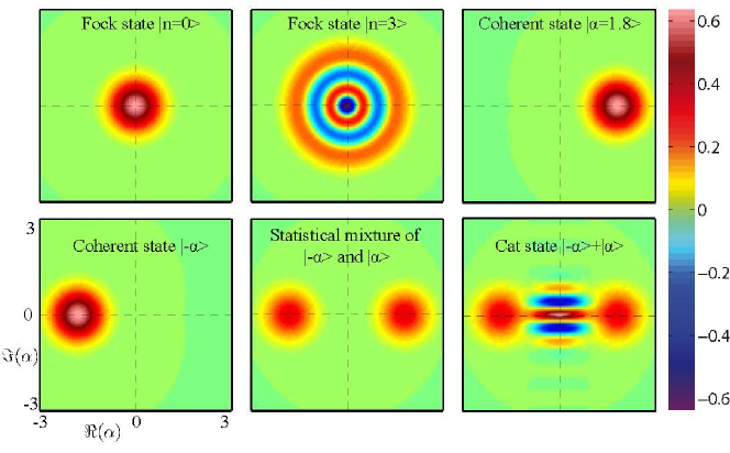
Figure 3: Wigner function of typical quantum states of an harmonic oscillator.

A possible definition of the Wigner function $W^{\rho}$ attached to any density operator $\rho$ is as follows:

$$W^{\rho}:{\mathbb{C}}\ni\alpha\rightarrow\tfrac{2}{\pi}\operatorname{Tr}\left(e^{i\pi{\boldsymbol{N}}}e^{-\alpha\boldsymbol{a}^{\dagger}+\alpha^{*}\boldsymbol{a}}\rho e^{\alpha\boldsymbol{a}^{\dagger}-\alpha^{*}\boldsymbol{a}}\right)\in[-2/\pi,2/\pi]$$

where $\alpha=x+ip$ is a position in the phase-plane $(x,p)$ of the classical oscillator. With the correspondences

$$\begin{split}&{\frac{\partial}{\partial\alpha}}=\tfrac{1}{2}\left({\frac{\partial}{\partial x}}-i{\frac{\partial}{\partial p}}\right),\quad{\frac{\partial}{\partial\alpha^{*}}}=\tfrac{1}{2}\left({\frac{\partial}{\partial x}}+i{\frac{\partial}{\partial p}}\right)\\ &W^{\rho\boldsymbol{a}}=\left(\alpha-\tfrac{1}{2}{\frac{\partial}{\partial\alpha^{*}}}\right)W^{\rho},\quad W^{\boldsymbol{a}\rho}=\left(\alpha+\tfrac{1}{2}{\frac{\partial}{\partial\alpha^{*}}}\right)W^{\rho}\\ &W^{\rho\boldsymbol{a}^{\dagger}}=\left(\alpha^{*}+\tfrac{1}{2}{\frac{\partial}{\partial\alpha}}\right)W^{\rho},\quad W^{\boldsymbol{a}^{\dagger}\rho}=\left(\alpha^{*}-\tfrac{1}{2}{\frac{\partial}{\partial\alpha}}\right)W^{\rho}\end{split}$$ (21)

the Lindblad-Kossakovki governing the evolution of the density operator $\rho$ of a quantum oscillator, with damping time constant $1/\kappa>0$ and resonant drive of real amplitude $u$,

$$\frac{d}{dt}\rho=u[\boldsymbol{a}^{\dagger}-\boldsymbol{a},\rho]+\kappa\left(\boldsymbol{a}\rho\boldsymbol{a}^{\dagger}-({\boldsymbol{N}}\rho+\rho{\boldsymbol{N}})/2\right),$$

becomes a convection-diffusion equation for the Wigner function $W^{\rho}$

$${\frac{\partial W^{\rho}}{\partial t}}=\tfrac{\kappa}{2}\left({\frac{\partial\leavevmode\nobreak\ }{\partial x}}\Big{(}(x-\bar{\alpha})W^{\rho}\Big{)}+{\frac{\partial\leavevmode\nobreak\ }{\partial p}}\Big{(}pW^{\rho}\Big{)}+\tfrac{1}{4}\Delta W^{\rho}\right)$$

where $\Delta$ denotes the Laplacian operator $\tfrac{\partial^{2}}{\partial x^{2}}+\tfrac{\partial^{2}}{\partial p^{2}}$. The solutions converge toward the Gaussian steady-state $W^{\overline{\rho}}(x,p)=\tfrac{2}{\pi}e^{-2(x-\bar{\alpha})^{2}-2p^{2}}$, where $\overline{\rho}=|\bar{\alpha}\rangle\langle\bar{\alpha}|$ is the coherent state of amplitude $\bar{\alpha}=2u/\kappa$.

Appendix B Qubit

The underlying Hilbert space $\mathcal{H}={\mathbb{C}}^{2}=\left\{c_{g}|{g}\rangle+c_{e}|{e}\rangle,\;c_{g},c_{e}\in{\mathbb{C}}\right\}$ where $(|g\rangle,|e\rangle)$ is the ortho-normal frame formed by the ground state $|g\rangle$ and the excited state $|e\rangle$. It is usual to consider the following operators on $\mathcal{H}$:

$$\begin{split}&\boldsymbol{\sigma_{\!\text{\bf-}}}=|{g}\rangle\langle{e}|,\quad\boldsymbol{\sigma_{\!\text{\bf+}}}=\boldsymbol{\sigma_{\!\text{\bf-}}}^{\dagger}=|{e}\rangle\langle{g}|,\quad{\boldsymbol{\sigma_{\!x}}}=\boldsymbol{\sigma_{\!\text{\bf-}}}+\boldsymbol{\sigma_{\!\text{\bf+}}}=|{g}\rangle\langle{e}|+|{e}\rangle\langle{g}|,\\ &\boldsymbol{\sigma_{\!y}}=i\boldsymbol{\sigma_{\!\text{\bf-}}}-i\boldsymbol{\sigma_{\!\text{\bf+}}}=i|{g}\rangle\langle{e}|-i|{e}\rangle\langle{g}|,\quad{\boldsymbol{\sigma_{\!z}}}=\boldsymbol{\sigma_{\!\text{\bf+}}}\boldsymbol{\sigma_{\!\text{\bf-}}}-\boldsymbol{\sigma_{\!\text{\bf-}}}\boldsymbol{\sigma_{\!\text{\bf+}}}=|e\rangle\langle e|-|g\rangle\langle g|.\end{split}$$ (22)

$\boldsymbol{\sigma_{\!x}}$, $\boldsymbol{\sigma_{\!y}}$ and $\boldsymbol{\sigma_{\!z}}$ are the Pauli operators. They are square root of $\boldsymbol{I}$: $\boldsymbol{\sigma_{\!x}}^{2}=\boldsymbol{\sigma_{\!y}}^{2}=\boldsymbol{\sigma_{\!z}}^{2}=\boldsymbol{I}.$ They anti-commute

$$\boldsymbol{\sigma_{\!x}}\boldsymbol{\sigma_{\!y}}=-\boldsymbol{\sigma_{\!y}}\boldsymbol{\sigma_{\!x}}=i\boldsymbol{\sigma_{\!z}},\quad\boldsymbol{\sigma_{\!y}}\boldsymbol{\sigma_{\!z}}=-\boldsymbol{\sigma_{\!z}}\boldsymbol{\sigma_{\!y}}=i\boldsymbol{\sigma_{\!x}},\quad\boldsymbol{\sigma_{\!z}}\boldsymbol{\sigma_{\!x}}=-\boldsymbol{\sigma_{\!x}}\boldsymbol{\sigma_{\!z}}=i\boldsymbol{\sigma_{\!y}}$$

and thus $[\boldsymbol{\sigma_{\!x}},\boldsymbol{\sigma_{\!y}}]=2i\boldsymbol{\sigma_{\!z}}$, $[\boldsymbol{\sigma_{\!y}},\boldsymbol{\sigma_{\!z}}]=2i\boldsymbol{\sigma_{\!x}}$, $[\boldsymbol{\sigma_{\!z}},\boldsymbol{\sigma_{\!x}}]=2i\boldsymbol{\sigma_{\!y}}$. The uncontrolled evolution is governed by the Hamiltonian $\boldsymbol{H}/\hbar={\omega\boldsymbol{\sigma_{\!z}}}/2$ where $\omega>0$ is the qubit pulsation. Thus the solution of $\frac{d}{dt}|\psi\rangle=-i\frac{\boldsymbol{H}}{\hbar}|\psi\rangle$ is given by

$$|\psi\rangle_{t}=e^{-i\left(\tfrac{\omega t}{2}\right)\boldsymbol{\sigma_{\!z}}}|\psi\rangle_{0}=\cos\left(\tfrac{\omega t}{2}\right)|\psi\rangle_{0}-i\sin\left(\tfrac{\omega t}{2}\right)\boldsymbol{\sigma_{\!z}}|\psi\rangle_{0}$$

since for any angle $\theta$ we have

$$e^{i\theta\boldsymbol{\sigma_{\!x}}}=\cos\theta+i\sin\theta\boldsymbol{\sigma_{\!x}},\quad e^{i\theta\boldsymbol{\sigma_{\!y}}}=\cos\theta+i\sin\theta\boldsymbol{\sigma_{\!y}},\quad e^{i\theta\boldsymbol{\sigma_{\!z}}}=\cos\theta+i\sin\theta\boldsymbol{\sigma_{\!z}}.$$

Since the Pauli operators anti-commute, we have the useful relationships:

$$e^{i\theta\boldsymbol{\sigma_{\!x}}}\boldsymbol{\sigma_{\!y}}=\boldsymbol{\sigma_{\!y}}e^{-i\theta\boldsymbol{\sigma_{\!x}}},\quad e^{i\theta\boldsymbol{\sigma_{\!y}}}\boldsymbol{\sigma_{\!z}}=\boldsymbol{\sigma_{\!z}}e^{-i\theta\boldsymbol{\sigma_{\!y}}},\quad e^{i\theta\boldsymbol{\sigma_{\!z}}}\boldsymbol{\sigma_{\!x}}=\boldsymbol{\sigma_{\!x}}e^{-i\theta\boldsymbol{\sigma_{\!z}}}.$$

The orthogonal projector $\rho=|\psi\rangle\langle\psi|$, the density operator associated to the pure state $|\psi\rangle$, obeys to the Liouville equation $\frac{d}{dt}\rho=-\tfrac{i}{\hbar}[\boldsymbol{H},\rho].$ Mixed quantum states are described by $\rho$ that are Hermitian, non-negative and of trace one. For a qubit, the Bloch sphere representation is a useful tool exploiting the smooth correspondence between such $\rho$ and the unit ball of ${\mathbb{R}}^{3}$ considered as Euclidian space:

$$\rho=\frac{\boldsymbol{I}+x\boldsymbol{\sigma_{\!x}}+y\boldsymbol{\sigma_{\!y}}+z\boldsymbol{\sigma_{\!z}}}{2},\quad(x,y,z)\in{\mathbb{R}}^{3},\quad x^{2}+y^{2}+z^{2}\leq 1.$$

$(x,y,z)\in{\mathbb{R}}^{3}$ are the coordinates in the orthonormal frame $(\vec{\imath},\vec{\jmath},\vec{k})$ of the Bloch vector $\vec{M}\in{\mathbb{R}}^{3}$. This vector lives on or inside the unit sphere, called Bloch sphere:

$$\vec{M}=x\vec{\imath}+y\vec{\jmath}+z\vec{k}.$$

Since $\operatorname{Tr}\left(\rho^{2}\right)=x^{2}+y^{2}+z^{2}$, $\vec{M}$ is on the Bloch sphere when $\rho$ is of rank one and thus is a pure state. The translation of Liouville equation on $\vec{M}$ yields with $\boldsymbol{H}/\hbar=\omega\boldsymbol{\sigma_{\!z}}/2$: $\frac{d}{dt}\vec{M}=\omega\vec{k}\times\vec{M}.$ For the two-level system with the coherent drive described by the complex-value control $u$, $\boldsymbol{H}/\hbar=\tfrac{\omega}{2}\boldsymbol{\sigma_{\!z}}+\tfrac{\Re(u)}{2}\boldsymbol{\sigma_{\!x}}+\tfrac{\Im(u)}{2}\boldsymbol{\sigma_{\!y}}$ and the Liouville equation reads, with the Bloch vector $\vec{M}$ representation,

$$\frac{d}{dt}\vec{M}=(\Re(u)\vec{\imath}+\Im(u)\vec{\jmath}+\omega\vec{k})\times\vec{M}.$$

Appendix C Jaynes-Cumming Hamiltonians and propagators

The Jaynes-Cummings Hamiltonian [36] is the simplest Hamiltonian describing the interaction between an harmonic oscillator and a qubit. Such an interaction admits two regimes, the resonant one where the oscillator and the qubit exchange energy, the dispersive one where the oscillator pulsation depends on the qubit state and where the qubit pulsation, slightly different from the oscillator pulsation, depends on the number of vibration quanta. We recall below the simplest forms of these Hamiltonians in the interaction frame. A deeper and complete presentation can be found in [33].

The resonant Hamiltonian $\boldsymbol{H}_{res}$ is given by

$$\boldsymbol{H}_{res}/\hbar=if(t)\leavevmode\nobreak\ \big{(}\boldsymbol{a}^{\dagger}\otimes\boldsymbol{\sigma_{\!\text{\bf-}}}-\boldsymbol{a}\otimes\boldsymbol{\sigma_{\!\text{\bf+}}}\big{)}=if(t)\leavevmode\nobreak\ \big{(}\boldsymbol{a}^{\dagger}\otimes|g\rangle\langle e|-\boldsymbol{a}\otimes|e\rangle\langle g|\big{)}$$ (23)

whereas the dispersive one $\boldsymbol{H}_{disp}$ is a simple tensor product:

$$\boldsymbol{H}_{disp}/\hbar=f(t)\leavevmode\nobreak\ {\boldsymbol{N}}\otimes\boldsymbol{\sigma_{\!z}}=f(t)\leavevmode\nobreak\ {\boldsymbol{N}}\otimes\big{(}|e\rangle\langle e|-|g\rangle\langle g|\big{)}$$ (24)

where $f(t)$ is a known real parameter depending possibly on the time $t$.

Simple computations show that the resonant propagator $\boldsymbol{U}_{res}$ between $t_{0}$ and $t_{1}$ associated to $\boldsymbol{H}_{res}$, i.e., the solution of Cauchy problem

$$\frac{d}{dt}\boldsymbol{U}=-i\frac{\boldsymbol{H}_{res}}{\hbar}\boldsymbol{U},\quad U(t_{0})=\boldsymbol{I},$$

is explicit and given by the following compact formulae:

$$\boldsymbol{U}_{res}(t_{0},t_{1})=\cos\left(\tfrac{\int_{t_{0}}^{t_{1}}f}{2}\sqrt{{\boldsymbol{N}}}\right)\otimes|g\rangle\langle g|+\cos\left(\tfrac{\int_{t_{0}}^{t_{1}}f}{2}\sqrt{{{\boldsymbol{N}}+\boldsymbol{I}}}\right)\otimes|e\rangle\langle e|\\ -\boldsymbol{a}\frac{\sin\left(\tfrac{\int_{t_{0}}^{t_{1}}f}{2}\sqrt{{\boldsymbol{N}}}\right)}{\sqrt{{\boldsymbol{N}}}}\otimes|e\rangle\langle g|\,+\frac{\sin\left(\tfrac{\int_{t_{0}}^{t_{1}}f}{2}\sqrt{{\boldsymbol{N}}}\right)}{\sqrt{{\boldsymbol{N}}}}\,\boldsymbol{a}^{\dagger}\otimes|g\rangle\langle e|.$$ (25)

It is instructive to check that $\boldsymbol{U}^{\dagger}_{res}\boldsymbol{U}_{res}=\boldsymbol{I}$. Similarly, the dispersive propagator $\boldsymbol{U}_{disp}$ between $t_{1}$ and $t_{2}$ associated to $\boldsymbol{H}_{disp}$ is given by

$$\boldsymbol{U}_{disp}(t_{0},t_{1})=\exp\left(i{\boldsymbol{N}}\int_{t_{0}}^{t_{1}}f\right)\otimes|g\rangle\langle g|+\exp\left(-i{\boldsymbol{N}}\int_{t_{0}}^{t_{1}}f\right)\otimes|e\rangle\langle e|.$$ (26)

Appendix D A positiveness-preserving numerical scheme

This appendix describes a positiveness-preserving formulation of the Euler-Milstein scheme for the numerical integration of stochastic master equations driven by a single Wiener process. They admit the following form

$$d\rho_{t}=\left(-\imath[\boldsymbol{H},\rho_{t}]+\sum_{\mu}\boldsymbol{L}_{\mu}\rho_{t}\boldsymbol{L}_{\mu}^{\dagger}-\tfrac{1}{2}(\boldsymbol{L}_{\mu}^{\dagger}\boldsymbol{L}_{\mu}\rho_{t}+\rho_{t}\boldsymbol{L}_{\mu}^{\dagger}\boldsymbol{L}_{\mu})\right)dt\\ +\bigg{(}\boldsymbol{L}\rho_{t}\boldsymbol{L}^{\dagger}-\tfrac{1}{2}(\boldsymbol{L}^{\dagger}\boldsymbol{L}\rho_{t}+\rho_{t}\boldsymbol{L}^{\dagger}\boldsymbol{L})\bigg{)}dt+\sqrt{\eta}\bigg{(}\boldsymbol{L}\rho_{t}+\rho_{t}\boldsymbol{L}^{\dagger}-\operatorname{Tr}\left(\boldsymbol{L}\rho_{t}+\rho_{t}\boldsymbol{L}^{\dagger}\right)\rho_{t}\bigg{)}dW_{t}$$ (27)

where $\rho$ is a square non-negative Hermitian matrix of trace $1$, $\boldsymbol{L}_{\mu}$ and $\boldsymbol{L}$ are square matrices, $W_{t}$ is a Wiener process and $\eta\in[0,1]$ is the detection efficiency. The measured continuous signal $y_{t}$ is given by $dy_{t}=\sqrt{\eta}\operatorname{Tr}\left(\boldsymbol{L}\rho_{t}+\rho_{t}\boldsymbol{L}^{\dagger}\right)dt+dW_{t}$.

For $dx=f(x)dt+g(x)dW_{t}$ ($x\in{\mathbb{R}}^{d}$ for some integer $d$, $f$ and $g$ smooth functions), the Euler-Milstein scheme (order $1$ in the discretization step denoted $dt$) reads [45]

$$x_{n+1}=x_{n}+f(x_{n})dt+g(x_{n})dW_{n}+\tfrac{1}{2}\frac{\partial g}{\partial x}(x_{n})\cdot g(x_{n})(dW_{n}^{2}-dt)$$

where $x_{n}$, for $n\in{\mathbb{N}}$, is an approximation of $x_{ndt}$ and $dW_{n}$ is a Gaussian variable with zero average and variance $dt$. For (27), we get

$$\rho_{n+1}=\rho_{n}+\left(-\imath[\boldsymbol{H},\rho_{n}]+\sum_{\mu}\boldsymbol{L}_{\mu}\rho_{n}\boldsymbol{L}_{\mu}^{\dagger}-\tfrac{1}{2}(\boldsymbol{L}_{\mu}^{\dagger}\boldsymbol{L}_{\mu}\rho_{n}+\rho_{n}\boldsymbol{L}_{\mu}^{\dagger}\boldsymbol{L}_{\mu})\right)dt\\ +\bigg{(}\boldsymbol{L}\rho_{n}\boldsymbol{L}^{\dagger}-\tfrac{1}{2}(\boldsymbol{L}^{\dagger}\boldsymbol{L}\rho_{n}+\rho_{n}\boldsymbol{L}^{\dagger}\boldsymbol{L})\bigg{)}dt+\sqrt{\eta}\bigg{(}\boldsymbol{L}\rho_{n}+\rho_{n}\boldsymbol{L}^{\dagger}-\operatorname{Tr}\left(\boldsymbol{L}\rho_{n}+\rho_{n}\boldsymbol{L}^{\dagger}\right)\rho_{n}\bigg{)}dW_{n}\\ +\tfrac{\eta}{2}\bigg{(}\boldsymbol{L}^{2}\rho_{n}+\rho_{n}(\boldsymbol{L}^{\dagger})^{2}+2\boldsymbol{L}\rho_{n}\boldsymbol{L}^{\dagger}-2\operatorname{Tr}\left(\boldsymbol{L}\rho_{n}+\rho_{n}\boldsymbol{L}^{\dagger}\right)(\boldsymbol{L}\rho_{n}+\rho_{n}\boldsymbol{L}^{\dagger})\ldots\\ -\big{(}\operatorname{Tr}\left(\boldsymbol{L}^{2}\rho_{n}+\rho_{n}(\boldsymbol{L}^{\dagger})^{2}\right)+2\operatorname{Tr}\left(\boldsymbol{L}\rho_{n}\boldsymbol{L}^{\dagger}\right)-2\operatorname{Tr}^{2}\left(\boldsymbol{L}\rho_{n}+\rho_{n}\boldsymbol{L}^{\dagger}\right)\big{)}\rho_{n}\bigg{)}(dW_{n}^{2}-dt).$$

Let us consider the following matrix

$$\boldsymbol{M}_{n}=\boldsymbol{I}-dt\left(i\boldsymbol{H}+\tfrac{1}{2}\sum_{\mu}\boldsymbol{L}_{\mu}^{\dagger}\boldsymbol{L}_{\mu}+\tfrac{1}{2}\boldsymbol{L}^{\dagger}\boldsymbol{L}\right)+\sqrt{\eta}\bigg{(}\sqrt{\eta}\operatorname{Tr}\left(\boldsymbol{L}\rho_{n}+\rho_{n}\boldsymbol{L}^{\dagger}\right)dt+dW_{n}\bigg{)}\boldsymbol{L}+\tfrac{\eta}{2}(dW_{n}^{2}-dt)\boldsymbol{L}^{2}.$$

Here $dW_{n}$ is of order $\sqrt{dt}$ and $dW_{n}^{2}-dt$ is of order $dt$. Then simple but slightly tedious computations up to $dt^{3/2}$ show that $\rho_{n+1}$ given by the above Euler-Milstein scheme reads also

$$\rho_{n+1}=\frac{\boldsymbol{M}_{n}\rho_{n}\boldsymbol{M}_{n}^{\dagger}+\sum_{\mu}\boldsymbol{L}_{\mu}\rho_{n}\boldsymbol{L}_{\mu}^{\dagger}dt+(1-\eta)\boldsymbol{L}\rho_{n}\boldsymbol{L}^{\dagger}dt}{\operatorname{Tr}\left(\boldsymbol{M}_{n}\rho_{n}\boldsymbol{M}_{n}^{\dagger}+\sum_{\mu}\boldsymbol{L}_{\mu}\rho_{n}\boldsymbol{L}_{\mu}^{\dagger}dt+(1-\eta)\boldsymbol{L}\rho_{n}\boldsymbol{L}^{\dagger}dt\right)}+O(dt^{3/2}).$$ (28)

When $\eta=0$, this expression provides, for any deterministic Lindblad differential equation, a positiveness-preserving formulation of the explicit Euler scheme.

References

• [1] C. Altafini and F. Ticozzi. Modeling and control of quantum systems: An introduction. Automatic Control, IEEE Transactions on, 57(8):1898–1917, 2012.
• [2] H Amini, C. Pellegrini, and P. Rouchon. Stability of continuous-time quantum filters with measurement imperfections. arXiv:1312.0418v1, 2013.
• [3] H. Amini, R.A. Somaraju, I. Dotsenko, C. Sayrin, M. Mirrahimi, and P. Rouchon. Feedback stabilization of discrete-time quantum systems subject to non-demolition measurements with imperfections and delays. Automatica, 49(9):2683–2692, September 2013.
• [4] S. Attal, A. Joye, and C.-A. Pillet, editors. Open Quantum Systems III: Recent Developments. Springer, Lecture notes in Mathematics 1880, 2006.
• [5] A. Barchielli and M. Gregoratti. Quantum Trajectories and Measurements in Continuous Time: the Diffusive Case. Springer Verlag, 2009.
• [6] S. M. Barnett and P. M. Radmore. Methods in Theoretical Quantum Optics. Oxford University Press, 2003.
• [7] L. Baudoin and J. Salomon. Constructive solution of a bilinear optimal control problem for a Schrödinger equation. Systems and Control Letters, 57:453––464, 2008.
• [8] L. Baudouin, O. Kavian, and J.P. Puel. Regularity for a Schrödinger equation with singular potentials and application to bilinear optimal control. J. Differential Equations, 216:188–222, 2005.
• [9] M; Bauer, T. Benoist, and D. Bernard:. Repeated quantum non-demolition measurements: Convergence and continuous time limit. Ann. Henri Poincare, 14:639––679, 2013.
• [10] K. Beauchard and J.-M. Coron. Controllability of a quantum particle in a moving potential well. J. of Functional Analysis, 232:328–389, 2006.
• [11] K. Beauchard, J.-M. Coron, and P. Rouchon. Controllability issues for continuous spectrum systems and ensemble controllability of Bloch equations. Communications in Mathematical Physics, 296:525–557, 2010.
• [12] K. Beauchard, P.S. Pereira da Silva, and P. Rouchon. Stabilization of an arbitrary profile for an ensemble of half-spin systems. Automatica, 49(7):2133–2137, July 2013.
• [13] V.P. Belavkin. Quantum stochastic calculus and quantum nonlinear filtering. Journal of Multivariate Analysis, 42(2):171–201, 1992.
• [14] G. Birkhoff. Extensions of Jentzch’s theorem. Trans. Amer. Math. Soc., 85:219–227, 1957.
• [15] B. Bonnard, O. Cots, S.J. Glaser, M. Lapert, D. Sugny, and Yun Zhang. Geometric optimal control of the contrast imaging problem in nuclear magnetic resonance. Automatic Control, IEEE Transactions on, 57(8):1957–1969, 2012.
• [16] L. Bouten and R. van Handel. Quantum Stochastics and Information: Statistics, Filtering and Control, chapter On the separation principle of quantum control. World Scientific, 2008.
• [17] P. Campagne-Ibarcq, E. Flurin, N. Roch, D. Darson, P. Morfin, M. Mirrahimi, M. H. Devoret, F. Mallet, and B. Huard. Persistent control of a superconducting qubit by stroboscopic measurement feedback. Phys. Rev. X, 3(2):021008–, May 2013.
• [18] H. . Carmichael. An Open Systems Approach to Quantum Optics. Springer-Verlag, 1993.
• [19] H. Carmichael. Statistical Methods in Quantum Optics 1: Master Equations and Fokker-Planck Equations . Springer, 1999.
• [20] H. Carmichael. Statistical Methods in Quantum Optics 2: Non-Classical Fields. Spinger, 2007.
• [21] T. Chambrion, P. Mason, M. Sigalotti, and M. Boscain. Controllability of the discrete-spectrum Schrödinger equation driven by an external field. Ann. Inst. H. Poincaré Anal. Non Linéaire, 26(1):329–349, 2009.
• [22] A. A. Clerk, M. H. Devoret, S. M. Girvin, Florian Marquardt, and R. J. Schoelkopf. Introduction to quantum noise, measurement, and amplification. Rev. Mod. Phys., 82(2):1155–1208, April 2010.
• [23] D. D’Alessandro. Introduction to Quantum Control and Dynamics. Chapman & Hall/CRC, 2008.
• [24] J. Dalibard, Y. Castion, and K. Mølmer. Wave-function approach to dissipative processes in quantum optics. Phys. Rev. Lett., 68(5):580–583, 1992.
• [25] E.B. Davies. Quantum Theory of Open Systems. Academic Press, 1976.
• [26] I. Dotsenko, M. Mirrahimi, M. Brune, S. Haroche, J.-M. Raimond, and P. Rouchon. Quantum feedback by discrete quantum non-demolition measurements: towards on-demand generation of photon-number states. Physical Review A, 80: 013805-013813, 2009.
• [27] S. Ervedoza and J.-P. Puel. Approximate controllability for a system of Schrödinger equations modeling a single trapped ion. Annales de l’Institut Henri Poincare (C) Non Linear Analysis, 26(6):2111 – 2136, 2009.
• [28] C.W. Gardiner and P. Zoller. Quantum noise. Springer, third edition, 2010.
• [29] A. Garon, S. J. Glaser, and D. Sugny. Time-optimal control of SU(2) quantum operations. Phys. Rev. A, 88(4):043422–, October 2013.
• [30] J. Gough and M.R. James. The series product and its application to quantum feedforward and feedback networks. Automatic Control, IEEE Transactions on, 54(11):2530–2544, 2009.
• [31] A. Grigoriu, H. Rabitz, and G. Turinici. Controllability analysis of quantum systems immersed within an engineered environment. Journal of Mathematical Chemistry, 51(6):1548–1560, 2013.
• [32] R. Hamerly and H. Mabuchi. Advantages of coherent feedback for cooling quantum oscillators. Phys. Rev. Lett., 109(17):173602–, October 2012.
• [33] S. Haroche and J.M. Raimond. Exploring the Quantum: Atoms, Cavities and Photons. Oxford University Press, 2006.
• [34] M.R. James. Quantum feedback control. In Control Conference (CCC), 2011 30th Chinese, pages 26–34, 2011.
• [35] M.R. James, H.I. Nurdin, and I.R. Petersen. H infinity control of linear quantum stochastic systems. Automatic Control, IEEE Transactions on, 53(8):1787–1803, 2008.
• [36] E.T. Jaynes and F.W. Cummings. Comparison of quantum and semiclassical radiation theories with application to the beam maser. Proceedings of the IEEE, 51(1):89–109, 1963.
• [37] A. Kastler. Optical methods for studying Hertzian resonances. Science, 158(3798):214–221, October 1967.
• [38] A. Kossakowski. On quantum statistical mechanics of non-Hamiltonian systems. Reports on Mathematical Physics, 3, 1972.
• [39] H.J. Kushner. Introduction to Stochastic Control. Holt, Rinehart and Wilson, INC., 1971.
• [40] Z. Leghtas. Quantum state engineering and stabilization. PhD thesis, Mines ParisTech, 2012.
• [41] G. Lindblad. On the generators of quantum dynamical semigroups. Communications in Mathematical Physics, 48, 1976.
• [42] S. Lloyd. Coherent quantum feedback. Phys. Rev. A, 62(2):022108–, July 2000.
• [43] H. Mabuchi and N. Khaneja. Principles and applications of control in quantum systems. International Journal of Robust and Nonlinear Control, 15(15):647–667, 2005.
• [44] J.C Maxwell. On governors. Proc. Roy. Soc. (London), 16, 1868.
• [45] G.N. Milstein. Numerical Integration of Stochastic Differential Equations. Spinger, 1995.
• [46] M. Mirrahimi, Z. Leghtas  , V.V. Albert, S. Touzard, R.J.. Schoelkopf, L. Jiang, and M.H. Devoret. Dynamically protected cat-qubits: a new paradigm for universal quantum computation. to appear in New Journal of Physics (arXiv:1312.2017v1), 2014.
• [47] M. Mirrahimi and R. Van Handel. Stabilizing feedback controls for quantum systems. SIAM Journal on Control and Optimization, 46(2):445–467, 2007.
• [48] M.A. Nielsen and I.L. Chuang. Quantum Computation and Quantum Information. Cambridge University Press, 2000.
• [49] N.C. Nielsen, C. Kehlet, S.J. Glaser, and N. Khaneja. Optimal control methods in nmr spectroscopy. In Encyclopedia of Nuclear Magnetic Resonance, pages –. John Wiley & Sons, Ltd, 2010.
• [50] D. Petz. Monotone metrics on matrix spaces. Linear Algebra and its Applications, 244:81–96, 1996.
• [51] J. F. Poyatos, J. I. Cirac, and P. Zoller. Quantum reservoir engineering with laser cooled trapped ions. Phys. Rev. Lett., 77(23):4728–4731, December 1996.
• [52] D. Reeb, M. J. Kastoryano, and M. M. Wolf. Hilbert’s projective metric in quantum information theory. Journal of Mathematical Physics, 52(8):082201, August 2011.
• [53] P. Rouchon. Fidelity is a sub-martingale for discrete-time quantum filters. IEEE Transactions on Automatic Control, 56(11):2743–2747, 2011.
• [54] S. Sarlette, M. Brune, J.M. Raimond, and P. Rouchon. Stabilization of nonclassical states of the radiation field in a cavity by reservoir engineering. Phys. Rev. Lett., 107:010402, 2011.
• [55] S. Sarlette, Z. Leghtas, M. Brune, J.M. Raimond, and P. Rouchon. Stabilization of nonclassical states of one and two-mode radiation fields by reservoir engineering. Phys. Rev. A, 86:012114, 2012.
• [56] C. Sayrin. Préparation et stabilisation d’un champ non classique en cavité par rétroaction quantique. PhD thesis, Université Paris VI, 2011.
• [57] C. Sayrin, I. Dotsenko, X. Zhou, B. Peaudecerf, Th. Rybarczyk, S. Gleyzes, P. Rouchon, M. Mirrahimi, H. Amini, M. Brune, J.M. Raimond, and S. Haroche. Real-time quantum feedback prepares and stabilizes photon number states. Nature, 477:73–77, 2011.
• [58] R. Sepulchre, A. Sarlette, and P. Rouchon. Consensus in non-commutative spaces. In Decision and Control (CDC), 2010 49th IEEE Conference on, pages 6596–6601, 2010.
• [59] A. Somaraju, I. Dotsenko, C. Sayrin, and P. Rouchon. Design and stability of discrete-time quantum filters with measurement imperfections. In American Control Conference, pages 5084–5089, 2012.
• [60] A. Somaraju, M. Mirrahimi, and P Rouchon. Approximate stabilization of an infinite dimensional quantum stochastic system. Rev. Math. Phys., 25(01):1350001–, January 2013.
• [61] R. van Handel. Filtering, Stability, and Robustness. PhD thesis, California Institute of Technology, 2007.
• [62] R. van Handel. The stability of quantum Markov filters. Infin. Dimens. Anal. Quantum Probab. Relat. Top., 12:153–172, 2009.
• [63] R. Vijay, C. Macklin, D. H. Slichter, S. J. Weber, K. W. Murch, R. Naik, A. N. Korotkov, and I. Siddiqi. Stabilizing Rabi oscillations in a superconducting qubit using quantum feedback. Nature, 490(7418):77–80, 2012.
• [64] H.M. Wiseman and G.J. Milburn. Quantum Measurement and Control. Cambridge University Press, 2009.
• [65] X. Zhou, I. Dotsenko, B. Peaudecerf, T. Rybarczyk, C. Sayrin, J.M. Raimond S. Gleyzes, M. Brune, and S. Haroche. Field locked to Fock state by quantum feedback with single photon corrections. Physical Review Letter, 108:243602, 2012.