Cold and warm atomic gas around the Perseus molecular cloud I: Basic Properties

Abstract

Using the Arecibo Observatory we have obtained neutral hydrogen (HI) absorption and emission spectral pairs in the direction of 26 background radio continuum sources in the vicinity of the Perseus molecular cloud. Strong absorption lines were detected in all cases allowing us to estimate spin temperature ($T_{s}$) and optical depth for 107 individual Gaussian components along these lines of sight. Basic properties of individual HI clouds (spin temperature, optical depth, and the column density of the cold and warm neutral medium, CNM and WNM) in and around Perseus are very similar to those found for random interstellar lines of sight sampled by the Millennium HI survey. This suggests that the neutral gas found in and around molecular clouds is not atypical. However, lines of sight in the vicinity of Perseus have on average a higher total HI column density and the CNM fraction, suggesting an enhanced amount of cold HI relative to an average interstellar field. Our estimated optical depth and spin temperature are in stark contrast with the recent attempt at using Planck data to estimate properties of the optically thick HI. Only $\sim 15$% of lines of sight in our study have a column density weighted average spin temperature lower than 50 K, in comparison with $\mathrel{\hbox{\hbox to0.0pt{\hbox{\lower 4.0pt\hbox{$\sim$}}\hss}\hbox{$>$}}}85$% of Planck’s sky coverage. The observed CNM fraction is inversely proportional to the optical-depth weighted average spin temperature, in excellent agreement with the recent numerical simulations by Kim et al. While the CNM fraction is on average higher around Perseus relative to a random interstellar field, it is generally low, $10-50$%. This suggests that extended WNM envelopes around molecular clouds, and/or significant mixing of CNM and WNM throughout molecular clouds, are present and should be considered in the models of molecule and star formation. Our detailed comparison of HI absorption with CO emission spectra shows that only 3/26 directions are clear candidates for probing the CO-dark gas as they have $N(HI)>10^{21}$ cm^-2 yet no detectable CO emission.

1 Introduction

Most of molecular gas in galaxies is assembled into giant molecular clouds (GMCs) with masses of 10⁴–10⁷ M_⊙ (Fukui & Kawamura, 2010). Stars appear intimately associated with the dense regions of these GMCs (Lada et al., 2010), and recent observations suggest that the depletion timescale of molecular gas by star formation does not vary greatly across a wide range of galaxy environments (Schruba et al., 2011; Shetty et al., 2014). This strongly suggests that the ability to form molecular gas in the first place holds the key to understanding the evolutionary tracks of galaxies.

Atomic hydrogen has been considered for decades as the main formation reservoir of GMCs (Shu, 1973; Blitz et al., 2007; Kim & Ostriker, 2006; Audit & Hennebelle, 2005; Heitsch et al., 2005; Clark et al., 2012). Although how exactly GMCs form out of the diffuse atomic medium is still not understood, the HI envelopes frequently observed around GMCs are likely to represent the material left over from the formation epoch and/or a product of photodissociation of molecular gas. In either case, these envelopes play a very important role in the GMC evolution and could explain long-standing questions such as the origin of the internal turbulent energy in GMCs. Theoretical models considering the ongoing accretion of atomic material from the envelope onto GMCs are able to reproduce the level of observed turbulence, as well as the total GMC mass (Chieze & Pineau Des Forets, 1989; Hennebelle & Inutsuka, 2006; Goldbaum et al., 2011). In addition, it has been suggested that the GMC history is highly dependent on the initial surface density of the HI envelope. As shown by Goldbaum et al. (2011), only a factor of two increase of the HI surface density of the envelope from 8 to 16 M_⊙ pc^-2 is enough to decide whether or not a GMC mass will reach $\sim 10^{6}$ M_⊙ over a typical lifetime of 10-20 Myr.

While the HI envelopes around molecular clouds have been largely observationally studied via HI emission (Wannier et al., 1983, 1991; Andersson & Wannier, 1993; Fukui et al., 2009), traditionally HI has not been considered as very important for understanding molecule and star formation. For example, many GMC studies trying to estimate the H₂ distribution from dust emission have neglected to account for HI as it was assumed that GMCs are highly dominated by molecular gas (e.g. Pineda et al. (2008)). In addition, a strong correlation between the star formation rate and the H₂ surface density in galaxies has been considered as an evidence that only H₂ is directly related to star formation. However, recent extragalactic studies showed that globally across galaxies at kpc-scales, as well as in resolved studies at sub-kpc scales, the HI surface density $\Sigma_{\rm H\textsc{i}}\mathrel{\hbox{\hbox to0.0pt{\hbox{\lower 4.0pt\hbox{$\sim$}}\hss}\hbox{$<$}}}$10 M_⊙ pc^-2 (Wong & Blitz, 2002; Blitz & Rosolowsky, 2004; Bigiel et al., 2008; Schruba et al., 2011), re-opening interest in the role of HI shielding in molecule formation.

To investigate the formation of H₂ from a theoretical point of view, and building up on several earlier studies (Spitzer & Jenkins, 1975; Elmegreen, 1993), Krumholz et al. (2009) (KMT09) considered the structure of a photodissociation region (PDR) in a spherical cloud that is embedded in a uniform and isotropic radiation field. Their model is based on the balance between H₂ formation on dust grains and photodissociation by Lyman–Werner (LW) photons and provides an analytic function for the H₂ fraction as a function of the gas surface density. Their most important prediction is that a certain amount of the Hi surface density, $\Sigma_{\rm H\textsc{i}}$, is required for shielding of H₂ against photodissociation. Once this minimum $\Sigma_{\rm H\textsc{i}}$ is achieved, additional Hi is fully converted into H₂ and therefore $\Sigma_{\rm H\textsc{i}}$ saturates while $\Sigma_{\rm H2}$ linearly increases. At solar metallicity, KMT09 predict $\Sigma_{\rm H\textsc{i}}\sim 10$ M_⊙ pc^-2 as the minimum $\Sigma_{\rm H\textsc{i}}$ required for H₂ formation, this is equivalent to the HI column density of $1.2\times 10^{21}$ cm^-2.

To investigate the role of HI shielding on sub-pc scales in Lee et al. (2012) we mapped the transition from Hi to H₂ across the Perseus molecular cloud. The HI data in this study were from the GALFA–Hi survey (Peek et al., 2011; Stanimirović et al., 2006) and the HI column density was estimated under the optically thin assumption. To estimate the H₂ image, the 60 and 100 $\mu$m data from the Improved Reprocessing of the IRAS Survey (IRIS) (Miville-Deschênes & Lagache, 2005) were used. We derived $T_{\rm dust}$ from the $I_{60}/I_{100}$ ratio, and then converted $\tau_{100}$ to $A_{V}$ by finding a proportionality constant between our derived $A_{V}$ and the $A_{V}$ image derived from optical extinction (provided by the COMPLETE survey, Ridge et al. (2006)). Finally, the H₂ column density was calculated as: $N$(H₂)= ($A_{V}$/DGR $-$ $N$(Hi))/2; the dust-to-gas ratio DGR = 1.1 $\times$ 10^-21 mag cm² was measured locally around Perseus.

The key result from Lee et al. (2012) is the detection of an almost constant $\Sigma_{\rm H\textsc{i}}$ of 6–8 M_⊙ pc^-2 for several dark and star-forming regions in Perseus. This is in agreement with KMT09’s prediction for the saturation of $\Sigma_{\rm H\textsc{i}}$. In addition, Lee et al. showed that H₂ extends up to 20 pc from core centers, and that the HI envelope is very extended ($>20$ pc). The HI halo of Perseus was previously studied by Andersson & Wannier (1993) who focused on dark region B5. Using radiative transfer modeling they found that the HI halo is about $5\times 8$ pc in size.

While the observed flattening of $\Sigma_{\rm H\textsc{i}}$ can be attributed to the conversion of Hi into H₂ as in KMT09, an alternative possibility is that $\Sigma_{\rm H\textsc{i}}$ is simply underestimated due to the presence of high optical depth HI which is not fully measured in emission line observations. The high optical depth HI can be measured from self-absorption features, caused by the background Galactic HI emission being absorbed by the cooler foreground HI (Knapp, 1974; Goodman & Heiles, 1994; Li & Goldsmith, 2003). Many narrow self-absorption features have been considered as kinematically associated with CO and have inferred temperature of less than 40 K and the atomic hydrogen column density fraction of only 0.0016 relative to H₂. If HI is a dissociation product of H₂, these measurements suggest a cloud age of 3–30 Myrs Goldsmith & Li (2005). While self-absorption can provide spatial information about the cold HI, e.g. Gibson et al. (2000), it always requires complicated line modeling and is limited by the ability to clearly distinguish self-absorption features from temperature fluctuations and/or multiple individual line of sight components.

The main aim of this study is to investigate the effect of high optical depth on the HI surface density saturation observed in Lee at al. (2012). We use the most direct way to estimate the “true” HI column density by measuring HI absorption against radio continuum sources located behind Perseus. We use these observations to investigate properties of the cold and warm HI around Perseus (Paper I), as well as to derive the ratio of the true HI column density to the HI column density derived under the optically thin assumption (Paper II).

The structure of this study is organized in the following way. In this paper (Paper I) we focus on the properties of cold gas around Perseus. Our observing and data processing strategies are explained in Section 2, and in Section 3 we summarize the methodology used to estimate spin temperature and column density of the cold neutral medium (CNM) and the warm neutral medium (WNM). In Section 4 we investigate the basic physical properties of atomic gas in the Perseus HI envelope, and in Section 5 we compare HI absorption and carbon monoxide (CO) emission spectra. We summarize our results in Section 6. In Paper II we estimate the correction for high optical depth using our HI absorption measurements, apply this correction and re-visit the question of HI saturation in Perseus.

2 Observations and Data Reduction

TABLE 1

Source list

Source	RA (J2000)	Dec (J2000)	$T_{src}$	$T_{sky}$
	(h m s)	(∘ ′ ′′)	(Jy)	(K)
NV0157+28	01:57:12.85	28:51:38.49	1.4	2.782
4C+29.05	02:01:35.91	29:33:44.18	1.2	2.785
4C+27.07	02:17:01.89	28:04:59.12	1.0	2.785
5C06.237	02:20:48.06	32:41:06.64	0.9	2.787
B20218+35	02:21:05.48	35:56:13.91	1.7	2.790
3C067	02:24:12.31	27:50:11.69	3.0	2.786
4C+34.07	02:26:10.34	34:21:30.45	2.9	2.791
NV0232+34	02:32:28.72	34:24:06.08	2.6	2.791
3C068.2	02:34:23.87	31:34:17.62	1.0	2.787
4C+28.06	02:35:35.41	29:08:57.73	1.3	2.788
4C+28.07	02:37:52.42	28:48:09.16	2.2	2.790
4C+34.09	03:01:42.38	35:12:20.84	1.9	2.794
4C+30.04	03:11:35.19	30:43:20.62	1.0	2.792
B20326+27	03:29:57.69	27:56:15.64	1.3	2.787
4C+32.14	03:36:30.12	32:18:29.47	2.7	2.793
3C092	03:40:08.55	32:09:02.32	1.6	2.791
3C093.1	03:48:46.93	33:53:15.41	2.4	2.795
4C+26.12	03:52:04.36	26:24:18.11	1.4	2.783
B20400+25	04:03:05.61	26:00:01.61	0.9	2.785
3C108	04:12:43.69	23:05:05.53	1.5	2.788
B20411+34	04:14:37.28	34:18:51.31	1.9	2.793
4C+25.14	04:20:49.30	25:26:27.63	1.0	2.785
4C+33.10	04:47:08.90	33:27:46.85	1.2	2.799
3C131	04:53:23.35	31:29:25.36	2.9	2.801
3C132	04:56:43.08	22:49:22.27	3.4	2.795
4C+27.14	04:59:56.10	27:06:02.19	0.9	2.796
3C133	05:02:58.51	25:16:25.16	5.8	2.796

2.1 HI absorption observations

We selected 27 radio continuum sources from the NVSS survey (Condon et al., 1998), located over an area of roughly 500 square degrees centered on Perseus with flux densities at 1.4 GHz greater than 0.8 Jy. Figure 1 shows the source positions overlaid on the H₂ surface density image of Perseus from Lee et al. (2012). Source information (RA, Dec, flux density at 21 cm, and the diffuse background radio continuum emission) is given in Table 1.

The observations were conducted with the Arecibo telescope. Using the L-wide receiver, we simultaneously recorded spectra centered at 1420 MHz and the two OH main lines (1665 and 1667 MHz), achieving a velocity resolution of 0.16 km s^-1. We sampled simultaneously two linearly polarized channels performing both auto and cross-correlations with the Arecibo’s three-level “interim” digital correlator. The Arecibo telescope has an angular resolution of 3.5^′ at these frequencies. As shown by Heiles & Troland (2003a) in their Millennium HI survey, Arecibo can accurately measure HI absorption lines for strong sources (flux density larger than $\sim 1$ Jy).

The observing procedure used was the same as in Heiles & Troland (2003a) and Stanimirović & Heiles (2005). This technique employs a 17-point observing pattern including 16 off-source measurements and one on-source measurement. The pattern was designed to measure the first and second derivatives of the 21-cm intensity fluctuations on the sky, and also to fine-tune for the instrumental effects involving the system gain. The auto-correlation data were used to derive the “expected” HI emission profile ($T_{exp}$), which is the profile that would be observed at the source position if the continuum sources were absent, the optical depth profile ($\tau$), and their uncertainties. With 17 measurements, the off-source spectra are expressed in a Taylor series expansion of the expected profile and a small contribution from the source intensity attenuated by the optical depth. A least-squares fitting technique is then used to estimate the optical depth profile, the expected profile and its spatial derivatives, and the off-source gain simultaneously (Heiles & Troland, 2003a). However, our updated data reduction software takes a slightly simpler approach by not including the fine-tuning of gain variations under the assumption that the on-axis telescope gain and the beam properties vary spatially and a detailed knowledge of these variations is required to estimate properly off-axis gains. Therefore, we just derive the optical depth profile, the expected profile and its spatial derivatives for each of 16 off positions. These are used to derive the uncertainty spectra for both the expected emission and optical depth spectra.

We have experimented with using the first order Taylor expansion instead of the second order. For all sources we find that the difference between optical depth profiles derived used the two expansions is within 1-$\sigma$ uncertainty. While the second order expansion is clearly more accurate (has smaller systematic errors), the derived $T_{exp}(v)$ and $\tau(v)$ are noiser than when using the first-order expansion. The increased noise comes from fitting a larger number of unknown parameters, and also from a large covariance between the second derivatives of the expected profile, $T_{exp}(v)$, and $\tau(v)$. We tolerate the slightly higher noise for better accuracy of derived profiles and therefore use the second-order Taylor expansion for all sources.

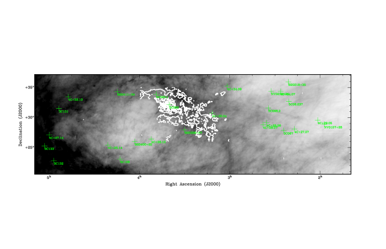
Figure 1: Positions of background radio continuum sources overlaid on the HI column density produced using GALFA-HI data at angular resolution of $\sim 4^{\prime}$. The intensity scale ranges from $2.2\times 10^{19}$ cm^-2 to $1.5\times 10^{21}$ cm^-2. White contours show the H₂ surface density distribution of Perseus from Lee et al. (2012). Contour levels range from 5 to 90% of the peak value ($4.6\times 10^{21}$ cm^-2), with a step of 10%.

Following the data reduction, for all sources we obtained an HI absorption spectrum ($e^{-\tau(v)}$), an HI (expected) emission spectrum ($T_{\rm exp}(v)$), and their uncertainty profiles. A main beam efficiency of $\eta=0.85$ (based on calibration measurements at Arecibo, Perillat et al.) was used to convert $T_{\rm exp}(v)$ from the antenna temperature units to the brightness temperature scale. With an integration time on average of about 1 hour, we achieved an rms noise level in optical depth of $\sim 1\times 10^{-3}$ per 1 km s^-1velocity channel.

Inspection of derived profiles revealed that several sources have small positive spectral features in their optical depth profiles at a level slightly higher than the 1-$\sigma$ uncertainty and highly localized in velocity. This effect is a result of high spatial derivatives of the HI emission (due to the presence of significant small-scale structure) and suggests that even the second-order Taylor expansion is not a good representation of the measured off positions in several cases. These sources are: 4C+27.14 and 4C+33.10. In addition, 4C+33.10 has very broad both absorption and emission profiles with many velocity components and its component fitting is more difficult and ambiguous than for other sources. However, in order to use as many sources as possible and considering that small artifacts are very localized in velocity, we include these three sources in our analysis (but make sure that artifacts are not fitted as real features). One source that we exclude from analysis is 4C+32.14 which has a highly saturated absorption profile and therefore all fitted parameters are highly uncertain for this source.

2.1.1 Comparison with HT03

Several of our sources were observed previously by Heiles & Troland (2003b) (from now on HT03): 3C+93.1, 3C131, 3C132, and 3C133. In terms of optical depth spectra, our results for 3C+93.1, 3C132, and 3C133 agree extremely well with HT03, within 3%. In the case of 3C131 we find a slightly larger difference, but this is still within the 3-$\sigma$ uncertainty. In case of expected profiles expressed in terms of antenna temperature, for all sources we find excellent agreement with HT03. We do correct our expected profiles for the beam efficiency and work with brightness temperature profiles in this paper.

2.2 HI emission data from the GALFA-HI survey

To investigate different methods for the derivation of the correction for high optical depth (focus of Paper II), as well as to estimate the importance of stray radiation, we also use the Hi emission data from the Galactic Arecibo L-band Feed Array Survey in Hi (GALFA–Hi). GALFA–Hi uses ALFA, a seven-beam array of receivers mounted at the focal plane of the 305-m Arecibo telescope, to map Hi emission in the Galaxy. Each of seven dual polarization beams has an effective beamsize of 3.9^′ $\times$ 4.1^′ and a gain of 8.5–11 Jy K^-1 (Peek et al., 2011). The GALFA–Hi spectrometer, GALSPECT, has a velocity resolution of 0.184 km s^-1 (872 Hz) and covers $-700$ km s^-1 $<v<$ $+700$ km s^-1 (7 MHz) in the Local Standard of Rest (LSR) frame.

In Lee et al. (2012) we combined scans from several GALFA-HI projects and produced an Hi cube of Perseus centered at (RA,Dec) = (03^h29^m52^s,$+$30^∘34^′1^′′) in J2000 with a size of 14.8^∘ $\times$ 9.0^∘. We use the same data here, but extend the data cube beyond Perseus to include locations of all radio continuum sources. This data cube has a size close to 60^∘ $\times$ 18^∘, with a pixel size of 1^′. After smoothing the cube to 36^′ and comparing the average HI spectrum with the corresponding spectrum from the Leiden/Argentine/Bonn (LAB) survey (Kalberla et al., 2005), we derived the correction factor of 1.1 that needed to be applied on the pixel-by-pixel basis to fine-tune GALFA-HI’s calibration (we note that our data came from an early data reduction scheme, before the public GALFA-HI data cubes were finalized and released).

Lee et al. (2012) also used the GALFA-HI data to investigate the HI saturation in Perseus. To estimate the HI column density, the Hi emission was integrated from $v_{\rm LSR}=-5$ to 15 km s^-1. This range was selected as resulting in the maximum correlation between $N$(Hi) and the A_V image from 2MASS (Ridge et al., 2006), exploring the idea that in mainly diffuse, low-A_V regions of Perseus where molecular gas is not abundant HI correlates well with A_V.

2.3 Stray radiation consideration for HI emission

Both our derived expected HI emission profiles and HI spectra from the GALFA-HI survey may be affected by stray radiation. Stray radiation is caused by radiation entering through higher order sidelobes and can result in broad, weak emission features. Correcting for stray radiation is a complex problem and requires a detailed knowledge of the Arecibo telescope beam and how it varies with azimuth and elevation. In this paper we provide only a rough check of our spectra relative to the LAB survey, which has been meticulously corrected for stray radiation. We take a twofold approach: (i) we compare our derived expected profiles $T_{exp}$ with the HI spectra from the GALFA-HI survey and find good agreement (within our estimated uncertainties); (ii) we then smooth the GALFA-HI data cube to the same angular and velocity resolution of the LAB survey (36^′), extract spectra at the positions of our continuum sources and compare them to search for broad wing-like features. We find that, in the majority of cases, the differences lie below the 1-$\sigma$ uncertainty level for our derived expected profiles. Therefore, we conclude that stray radiation is not a significant problem for this study. Our future work will develop a methodology for a detailed stray radiation correction.

Figure 2: (left) Brightness temperature of expected profiles of all sources offset in y-axis by 15 K for comparison. (right) Optical depth profiles of all sources offset in y-axis by 0.8 for easy comparison.

2.4 Additional data sets

We use the CO (1-0) emission data from Dame et al. (2001) obtained with the 1.2 m telescope at the Harvard Smithsonian Center for Astrophysics (CfA) and at 8.4^′ angular resolution. We also use the integrated CO intensity ($W_{CO}$) and $E(B-V)$ images from Planck (Planck Collaboration et al., 2013) with angular resolution of 5^′. When using Planck data for comparison with Dame et al. (2001) we first smooth the Planck images to angular resolution of 8^′ and regrid to make sure pixels are independent.

3 Analysis: Component fitting of HI absorption/emission pairs

To analyze HI absorption spectra we performed a decomposition into individual velocity components by employing the technique of Heiles & Troland (2003a). This allows us to estimate spin temperature and the HI column density for individual CNM components. This technique assumes that the CNM contributes to both HI absorption and emission spectra, while the warm neutral medium (WNM) contributes only to the HI emission spectrum. The technique is based on the Gaussian decomposition of both absorption and emission spectra, and it takes into account the fact that a certain fraction of the WNM gas may be located in front of the CNM clouds, resulting in a portion of the WNM being absorbed by the CNM. All possible permutations of the CNM components along the line-of-sight have been taken into account when searching for the best fit. Pros and cons regarding the use of Gaussian functions to represent the CNM absorption profiles have been discussed in Heiles & Troland (2003a).

We first fit $\tau(v)$ with a set of $N$ Gaussian functions using a least-squares technique:

$$\tau(v)=\sum_{0}^{N-1}\tau_{0,n}e^{-[(v-v_{0,n})/\delta v_{n}]^{2}}$$ (1)

where $\tau_{0,n}$ is the peak optical depth, $v_{0,n}$ is the central velocity, and $\delta v_{n}$ is the 1/e width of component $n$. $N$ is the minimum number of components necessary to make the residuals of the fit smaller or comparable to the estimated noise level of $\tau(v)$.

While the optical depth spectrum predominantly reflects the CNM, both the cold and warm neutral media contribute to the expected HI emission spectrum:

$$T_{\rm exp}(v)=T_{B,CNM}(v)+T_{B,WNM}(v).$$ (2)

The first term, $T_{B,CNM}(v)$, the HI emission originating from $N$ CNM components is:

$$T_{B,CNM}(v)=\sum_{0}^{N-1}T_{s,n}(1-e^{-\tau_{n}(v)})e^{-\sum_{0}^{M-1}\tau_{m}(v)},$$ (3)

where $T_{s,n}$ is the spin temperature of cloud $n$, and the subscript $m$ represents each one of the $M$ CNM clouds that lie in front of cloud $n$.

Next, $T_{B,WNM}(v)$, the HI emission originating from the WNM, is represented with a set of $K$ Gaussian functions. The complicating factor here is that a certain fraction $F$ of the WNM is located in front of the CNM, while a fraction $(1-F)$ of the WNM is beyond the CNM with its emissions being absorbed by CNM clouds:

$$T_{B,WNM}(v)=\sum_{0}^{K-1}[F_{k}+(1-F_{k})e^{-\tau(v)}]\times T_{0,k}e^{-[(v-v_{0,k})/\delta v_{k}]^{2}},$$ (4)

where the subscript $k$ corresponds to each of the WNM components and a fraction $F_{k}$ of the WNM cloud $k$ lies in front of all CNM components, while a fraction $1-F_{k}$ is being absorbed by the CNM clouds. To fit the corresponding emission spectra, we assume that the center and width of the absorption-selected CNM components are fixed and include a minimum number of additional WNM components to reduce the fit residuals to within the neighborhood of the 1-$\sigma$ uncertainties. We use a certain number of WNM components and fit the $T_{\rm exp}(v)$ profile simultaneously for the Gaussian parameters of the WNM components and the spin temperature of individual CNM clouds, while assuming a given order of CNM clouds along the line of sight and a given set of $F_{k}$ values. We try to use the minimum number of WNM components such that the residuals of this fitting process are reasonably close to the 1-$\sigma$ uncertainty for $T_{\rm exp}$.

Please note that the expected profile in the left-hand side of equation (2) has been baseline corrected, which means that we measure $T_{\rm exp}(v)-T_{sky}$, where $T_{sky}$ contains contributions from the Cosmic Microwave Background (CMB) and the Galactic synchrotron emission. Before doing the radiative transfer calculations we estimate $T_{sky}$ and add it back to the left-hand side of equation (2) by assuming 2.725 K for the CMB. To estimate the contribution from the Galactic synchrotron emission we use the Haslam et al. (1982) 408 MHz survey of the Galaxy. The brightness temperature at 408 MHz is converted to 1.4 GHz using the spectral index of $-2.7$. As the Galactic latitude of observed sources in the vicinity of Perseus is generally $>10$ degrees, the synchrotron contribution is small and $T_{sky}$ ranges from 2.78 to 2.80 K in our case (Table 1).

For each source, we vary the order of Gaussian functions along the line-of-sight (for $N$ CNM components there are $N!$ possible orderings) and perform the $T_{\rm exp}(v)$ fit. We then choose the ordering of CNM components that gives the smallest residuals in the least-squares fit. Unfortunately, the difference in the fit residuals is often not sufficiently statistically significant to distinguish between different values of $F_{k}$. However, $F_{k}$ has a large effect on the derived spin temperatures. Hence we follow the Heiles & Troland (2003a) suggestion and estimate the final spin temperatures by assigning characteristic values of 0, 0.5, or 1 to each $F_{k}$ (among the extreme possible values of 0 and 1), and repeating this for all possible combinations of WNM clouds. The final spin temperatures are then derived as a weighted average over all trials.

Out of 26 sources, 23 have well-constrained fits. Three sources, 3C133, 3C131 and 4C+25.14, have more than 6 individual CNM components in their absorption spectra. The corresponding fit for the spin temperature of these components in the presence of WNM features in emission is therefore more complicated, and the fitting process does not converge. Furthermore, for 6 sources (3C068.2, 3C133, 4C+25.14, 4C+28.07, 4C+30.04, and B20411+34) the fitted height of one absorption component is too small to be reliably recovered in the corresponding emission spectrum. Thus, the spin temperatures for these 6 components are calculated to be less than 1 K. Increasing the spin temperature by hand does not significantly degrade the quality of the fit. Therefore, for these uncertain components, we set the spin temperature equal to the uncertainty in $T_{s}$ derived from the iterations over CNM component orders along the line of sight and fraction of WNM absorbed. The error on this value is set to the median $T_{s}$ error for components along all 26 lines of sight, or 6.75 K.

Figure 3: Example Gaussian fits to emission and absorption spectra. (Left) 3C131, (Right) 4C+27.14. In the top panels, the thin solid line is the expected profile, $T_{\mathrm{exp}}$ (see Section 2.1 for derivation). The thin dot-dashed lines display the sum of WNM Gaussian components and the thick dashed lines display the total contribution to the $T_{\mathrm{exp}}$ profile by the CNM from the absorption profile. The thick solid line is the total WNM and CNM fit. The residuals from the fit are plotted below zero, with +/- $\Delta T_{\mathrm{exp}}$ overplotted. In the bottom panel, the thin solid line shows the optical depth profile ($e^{-\tau}$), with CNM components displayed in the thin dotted lines and the thick solid line representing the fit to the optical depth profile. The residuals from the fit are plotted at the bottom of the figure, with +/- $\Delta e^{-\tau}$ overplotted.

Figure 4: Example Gaussian fits to emission and absorption spectra. (Left) 3C092 which is located behind the main body of Perseus, (Right) NV0157+28. See Figure 3 for a detailed description of the panels.

4 Properties of cold and warm gas around Perseus

Figure 2 shows emission and absorption spectra for all sources except 4C+32.14 which has a saturated optical depth profile. Strong absorption lines were detected in the direction of all sources. In all cases, the strongest emission and absorption is found at $\sim 0$ km s^-1, and is generally well confined within the range of $-20$ to 20 km s^-1(see also Figure 6). However, in the case of four sources (4C+33.10, 4C+27.14, 3C133, and 3C131) there are strong emission and absorption features around $-40$ km s^-1. Visual inspection of velocity components close to Perseus using the GALFA-HI data cubes suggests that this secondary region is likely not associated with Perseus.

We show results of our Gaussian component fitting for 4 example sources in Figures 3 and 4. In each panel of both figures we plot the derived expected emission and optical depth profiles for an individual source. For the optical depth spectra, we overplot the individual CNM components (dotted lines), as well as the residuals for the fit (offset to the bottom of the panel) with the derived uncertainties for the spectrum for comparison. For the expected emission profiles, we overplot the sum of all WNM components (dot-dashed line), the total $T_{s}$-corrected contribution of the CNM (thick dashed line), and the fit residuals (shown below zero in the panel) with the uncertainties in the profile for comparison. The two sources in Figure 3, 3C131 and 4C+27.14, have broad HI profiles as likely include emission/absorption beyond Perseus, 3C092 in Figure 4 is located behind the main body of Perseus, and NVO0157+26 in the same figure is an example of a low optical depth profile.

In Table 2, we list the Gaussian parameters associated with all CNM and WNM components for each source. In column 1 we list the peak brightness temperature for each component. For the WNM components, this is equal to the unabsorbed Gaussian height and estimated error in the fit. For the CNM components, this is equal to the calculated spin temperature multiplied by (1-$e^{-\tau}$), as in Equation 3, and is quoted without uncertainty. In columns 2 and 3 we list the centers and FWHM of CNM and WNM components with estimated fit uncertainties. In column 4, we list the peak optical depth of each component. For the CNM components, this is equal to the height of each component (in $\tau$), with associated uncertainty. For the WNM components, this is equal to the maximum contribution of each WNM component detected in emission to the absorption profile, and is found by measuring the height of the absorption fit residuals at the central velocity of each WNM component. In column 5 we list the spin temperatures, which for the CNM components is equal to the calculated values from the fit with fit uncertainties. For the WNM components, this is equal to a lower limit imposed by the upper limit on optical depth in column 4, and these values are also quoted without error because the errors are extremely large due to the nature of the estimation process. In column 6, we list the maximum kinetic temperature of each component based on the line widths. In column 7, we list the HI column density of each individual component, and these values are quoted in units of 10²⁰ cm^-2. Finally, in column 8 we list the fraction of each WNM component lying in front of all CNM components ($F$, either 0.0, 0.5 or 1.0, see Section 2.2) or the order of each CNM component along the line of sight ($O$, integer values).

4.1 Optical Depth

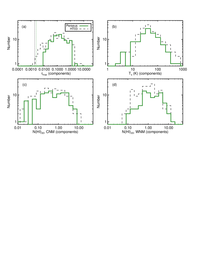
Figure 5: Histograms of Gaussian fit parameters for individual Gaussian components: (a) peak optical depth $\tau_{\rm max}$, (b) spin temperature, (c) the CNM column density (in units of $10^{20}$ cm^-2), and (d) the WNM column density (in units of $10^{20}$ cm^-2). Gaussian components from the HT03 survey at $|b|>10$ degrees are shown with a dashed black line for comparison. Dotted lines show the median sensitivity in optical depth for two studies. We assume here as the CNM all HI detected in absorption.

A summary of the fitting results is presented in Figures 5 to 8. As shown in Figure 5 (a), the median peak optical depth $\tau_{max}$ for individual Gaussian components is 0.16, and only a handful of CNM components has $\tau_{max}>1$ (10/107). Perseus is an intermediate-mass GMC located about 20 degrees below the Galactic plane and may not sample the densest molecular gas. In addition, a tighter grid of background sources may be able to sample better denser gas. Only two of our sources are located right behind the main body of Perseus. Their peak optical depth is 1.5.

The same figure shows $\tau_{max}$ for the components from HT03, dotted lines show median rms noise in optical depth for two studies. The two studies agree very well and have relatively similar (median) sensitivity, but we are missing the low-$\tau_{max}$ portion of the distribution. This could be partially due to our small survey area relative to HT03 who had more sources at high Galactic latitudes. We note that HT03’s sensitivity varies across sources as their survey was searching for strong sources suitable for Zeeman measurements.

Very recently, Fukui et al. (2014b) suggested a new approach to estimate properties (optical depth and spin temperature) of cold HI by utilizing dust emission. They noticed that the Planck dust optical depth $\tau_{353}$ at 353 $\mu$m correlates with $N(HI)$, but the scatter in this relation is much smaller when different dust temperature regimes are considered separately. By assuming that the highest dust temperature sub-sample is associated with the optically-thin HI, the saturation seen in the $\tau_{353}$-$N(HI)$ relation was attributed to the existence of the high optical depth HI solely. By inverting the relation, they estimated a single value of $T_{s}$ and $\tau_{HI}$ per pixel from their all-sky $\tau_{353}$ images (after masking low-latitude regions with $|b|<15$ degrees and regions with internal dust heating as traced by the H$\alpha$ emission). They found that 85% of data points have $\tau_{HI}>0.5$ and $T_{s}<40$ K. Similar results were obtained for the high latitude clouds MBM 53-55 (Fukui et al., 2014a), increasing the HI mass of MBM 53-55 clouds by a factor of two. Fukui et al. (2014b) suggested that the local interstellar medium (ISM) may be dominated by the high optical depth HI, and that this component may explain all of the CO-dark gas in the Milky Way.

Around Perseus we find $\tau_{max}>0.5$ only for 21 out of 107 (20%) individual (Gaussian) components. This is clearly in stark contrast with Fukui et al. (2014b) who claimed that 85% of lines of sight at essentially $|b|>15$ degrees have $\tau>0.5$ based on their comparison of $\tau_{353}$ and $N(HI)$.

4.2 Spin Temperature

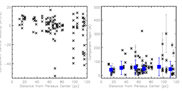
Figure 6: (Left) The central velocity of all Gaussian components showing that most components are found within $-20$ to 20 km s^-1  velocity range. (Right) The spin temperature of Gaussian components with velocity centroid within $-20$ and 20 km s^-1  shown as a function of distance from the Perseus center. Squares show median values of $T_{s}$ calculated over 20 pc wide distance bins. The angular separation has been converted into linear distance assuming a distance of 300 pc.

Figure 5 (b) shows our estimated spin temperature which ranges from $\sim 5$ to 725 K, with most CNM components having $T_{s}=10$ to 200 K. The spin temperature distribution peaks at $\sim 50$ K, the median value is 49 K. This is in excellent agreement with HT03 results based on 66 random lines of sight at $|b|>10^{\circ}$, as shown in the same figure. While we have a slightly smaller number of components relative to the HT03 study, the agreement between two studies is excellent over the full temperature range. In summary, the component spin temperature, for the predominantly CNM population we are tracing in absorption, is similar between a large angular area and a more focused area around Perseus.

In addition to HT03, one of our sources, 3C093.1, was observed by Andersson et al. (1992) who found only one absorption component and estimated its spin temperature of 41 K. The line of sight to this source pierces through the main body of Perseus. We have fitted the HI absorption spectrum with three components, and their spin temperature is $45\pm 13$, $44\pm 17$ and $23\pm 11$, respectively. The range of spin temperature in the direction of additional seven sources observed by Andersson, Roger, Wannier (1992) is $40-100$ K. This all shows that our derived temperatures are in general agreement with previous studies. Our mean $T_{s}$ is also in agreement with an estimate from Lee et al. (2012) of 60-75 K, where the equilibrium KMT09 model for the H₂ fraction was fitted to observations, under the overarching assumption of the CNM and WNM co-existing in pressure equilibrium.

In stark contrast to Fukui et al. (2014b), we find the spin temperature distribution essentially identical to an average CNM temperature distribution for the Milky Way, e.g. HT03 or Strasser et al. (2007). Out of 107 absorption-detected Gaussian components, $\sim 50$% have $T_{s}<50$ K. There are three sources whose projected distance from the rough center of Perseus is less than 20 pc, and their mean spin temperature is 45 K. The low spin temperature (20-40 K for 85% of data points) in Fukui et al. could be an artifact of neglecting to account for the “CO-dark” H₂ gas in the $\tau_{353}$-N(HI) correlation, and the use of line-of-sight averaged properties (single spin temperature and optical depth).

In Figure 6 (left) we show the central velocity of all Gaussian CNM components which shows that most components have a central velocity between $-20$ and 20 km s^-1. In Figure 6 (right) we plot $T_{s}$ for all components within this velocity range, excluding components that are likely (based on their central velocity) not associated with Perseus. Squares show median $T_{s}$ over 20 pc wide bins. We do not find obvious variations of $T_{s}$ with the distance from the center of Perseus.

Spatial changes of $T_{s}$ across interstellar clouds have been claimed in the literature. Liljestrom & Mattila (1988) mapped the HI distribution of a high latitude cloud and interpreted the observed increase in the line width as being due to an increase of $T_{s}$ by $\sim 30$ K. Andersson, Roger, Wannier (1992) performed radiative transfer modeling of HI observations of the B5 region in Perseus, considering internal stars and the effect of stellar winds on the spin temperature distribution. Their model suggests spin temperature of 40-50 K within the first 2 pc from the central star cluster, and then an increase to 200-300 K out to 6-8 pc from the core center. We do not find any evidence for a systematic change of $T_{s}$ radially from the Perseus center as shown in Figure 6, however we have large gaps in the background source coverage. A much tighter grid of HI absorption spectra within 50 pc from the center would be important for future studies.

4.3 HI column density and the CNM fraction

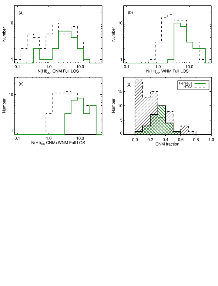
Figure 7: Histograms of basic properties calculated for each line of sight, from this study as solid green and from HT03 (for their $|b|>10^{\circ}$ sources) as dashed black: (from top left to bottom right) the CNM column density, the WNM column density, the CNM+WNM column density, and the CNM fraction (CNM/(CNM+WNM) column density). A $T_{s}$ threshold of 200 K was applied when selecting CNM components.

Histograms of the CNM and WNM column densities derived for individual Gaussian components are shown in Figure 5 (c) and (d) as solid green, while the results from the HT03 survey are shown as dashed black. There is excellent agreement between two studies. Our median CNM column density is $6.0\times 10^{19}$ cm^-2, in comparison to $5.2\times 10^{19}$ cm^-2 by HT03. Our median WNM column density is $1.5\times 10^{20}$ cm^-2, in good agreement with $1.3\times 10^{20}$ cm^-2 estimated by HT03. Please note that both studies treated as the CNM all HI detected in absorption and no temperature selections were made to distinguish the CNM from the thermally unstable WNM. It is interesting to note that Figure 5 shows that the WNM has a more uniform column density, while the CNM column density varies more dramatically, from $10^{18}$ to $10^{21}$ cm^-2.

In Figure 7 we show integrated CNM and WNM properties for different lines of sight probed by our target background sources, as well as results from HT03 for their 66 random directions at $|b|>10^{\circ}$. As several of our CNM components have higher temperature likely more appropriate for the thermally unstable WNM (e.g. Kim et al. 2014), we have applied a temperature threshold of $T_{s}<200$ K when calculating the CNM column density and the CNM fraction along the line of sight. The same threshold was applied for the HT03 data.

The main conclusion from this figure is that the line of sight properties in our study trace the upper range of the HT03 histograms. In terms of details, we find median CNM and WNM HI column density of $4.5\times 10^{20}$ cm^-2 and $7.8\times 10^{20}$ cm^-2, respectively. Both values are more than five times higher than the corresponding median values in HT03. The same applies to the total HI column density. To quantify the disagreement between our study and HT03 we have calculated cumulative distribution functions for all distributions in Figure 7. The K-S test suggests that there is $\mathrel{\hbox{\hbox to0.0pt{\hbox{\lower 4.0pt\hbox{$\sim$}}\hss}\hbox{$<$}}}3$% probability that Perseus and HT03 line-of-sight distributions were drawn from the same sample.

HT03 found a large number of sources with $\Sigma N(HI)_{CNM}=0$ as can be seen in Figure 7(d) where $\sim 15$ of HT03’s sources did not have detectable CNM. Stanimirović & Heiles (2005) and Stanimirović et al. (2007) showed that with $>4$ times longer integrations weak CNM features were detected in some of these directions. For each of our 26 sources we detect significant HI absorption lines with the CNM fraction being $>20$% for 20 sources, the lowest CNM fraction we find is 1% and there is only one source with such low fraction. As the sensitivity of two studies is on average similar, our higher fraction of absorbing HI likely stems from the intrinsic properties of the Perseus region. Our median CNM fraction is 0.33, in comparison to 0.22 in HT03 (after the same 200 K cut-off was applied to both studies). The above results strongly suggest that the Perseus region has a higher fraction of absorbing HI and a higher total HI column density relative to an average ISM field. The absorbing HI appears to contribute significantly to the total column density along almost every line of sight.

In summary, while properties of individual components are in excellent agreement with those of HT03, it appears that the Perseus region has a larger number of absorbing HI components relative to an average, random ISM field. This could explain the enhanced total HI column density and the fraction of the absorbing HI. Our results in particular for the CNM (and to a smaller degree for the WNM) and the total $N(HI)$ essentially trace the upper range of the corresponding distributions from HT03.

The CNM fraction, and especially its variations with interstellar environments, are poorly constrained observationally. In a comprehensive study of 290 HI emission/absorption pairs, Dickey et al. (2009) showed that the radial dependence of the harmonic mean spin temperature, which is a product of the spin temperature and the CNM fraction, is flat across the Milky Way disk. Considering that Strasser et al. (2007) showed that spin temperature of the CNM is similar between the inner and outer Galaxy, this result implies a nearly constant CNM fraction out to 25 kpc. Our study of Perseus is the first hint that the CNM fraction in/around GMCs is likely higher than what is found in an average ISM field.

4.4 What determines the CNM fraction?

While the Perseus region has on average a higher CNM fraction relative to an average ISM field, as shown in Figure 7, interestingly almost all directions (25/26) in our study have the CNM fraction smaller than 50%. We emphasize that this result is not an artifact of our applied $T_{s}<200$ K cutoff. If we do not apply any temperature cutoff, the median CNM fraction is 35%, and 23/26 directions have a CNM fraction $<50$%.

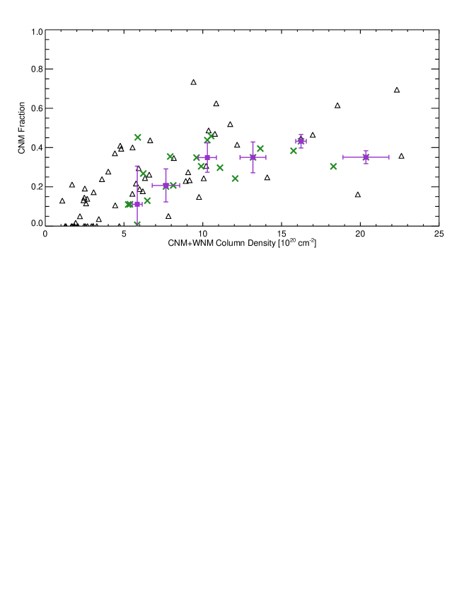
Figure 8: The CNM fraction as a function of the total HI column density, green crosses show our data and black triangles are from HT03. Purple points show median values with 1-$\sigma$ scatter calculated for our observations only. To isolate CNM-only and exclude potentially thermally-unstable WNM we have applied a cutoff $T_{s}<200$ K for both data sets.

In Figure 8 we show the CNM fraction as a function of the total HI column density for our sources as well as HT03 data. It is obvious that the CNM fraction never gets higher than $\sim 80$% (for both studies). This shows that there are no lines of sight without the WNM, even in the directions where the CNM hugely dominates the WNM fraction is at least $\sim 20$%. Although the scatter in this figure is large, the CNM fraction appears to increase from 0 to $\sim 40$% at $N(HI)\sim 10^{21}$ cm^-2, and then levels off (purple points show median values for Perseus observations). As pointed out by Heiles & Troland (2003b), this transition occurs right around the column density required for shielding H₂, suggesting that the CNM transitions into H₂ as soon as the adequate shielding is achieved. This column density also agrees with Lee et al. (2012) who showed that the HI-to-H₂ transition (defined as having a H₂ fraction of 0.25) occurs in Perseus at $N(HI)=(6-12)\times 10^{20}$ cm^-2.

In Figure 9 (top) crosses show the CNM fraction as a function of the column density weighted average spin temperature along the line of sight. A recent study by Kim et al. (2014), which produced synthetic HI spectra based on their 3D hydrodynamic simulations of a Milky Way-like disk, suggested that for the observed $T_{s}<400$ K the CNM fraction is proportional to the inverse of $T_{s}$. While their synthetic spectra represent random directions, most of the simulated data are located between $50K/T_{s}$ and $100K/T_{s}$ lines. Furthermore, for the observed $T_{s}<200$ K the simulated CNM fraction ranges between 40% and 70%, with a median value being 52% (97% of simulated data points have a CNM fraction $<70$%, Kim et al. private communication). We overplot the $1/T_{s}$ relation in the figure for three representative temperature values of 20, 50 and 100 K (the simulation applied a CNM temperature cut-off of $T_{k}<184$ K, where $T_{k}$ is the true kinetic temperature ). To bracket most of our data points we need to expand the $T_{s}$ range to lower temperatures of $\mathrel{\hbox{\hbox to0.0pt{\hbox{\lower 4.0pt\hbox{$\sim$}}\hss}\hbox{$<$}}}20$ K. With our observed CNM fraction being largely in the range of 10-50%, we overlap with the 40-70% range expected by the simulation although, the simulated fraction is generally slightly higher than what we observe. Square symbols in this plot show the difference introduced in the CNM fraction when a 350 K threshold is applied (instead of 200 K) to select the CNM. The difference is very small, only three data points are noticeably affected.

In the same figure (bottom panel) instead of using our calculated $T_{s}$ we follow exactly Kim et al. (2014) and calculate the observed temperature as the optical-depth weighted average spin temperature along the line of sight (equation (15) from Kim et al.). Most of our data points follow the 50/$T_{s}$ line, which agrees well with our median $T_{s}$ estimate, and is in excellent agreement with the Kim et al (2014) prediction. Considering that in the simulation the CNM fraction is known, while the observed CNM fraction is based on the Gaussian-decomposition $T_{s}$ derivation method, this excellent agreement is an indirect evidence that the observational method provides consistent and reliable CNM fractions.

While the optical-depth weighted average spin temperature (shown in the bottom panel) is on average higher than our column density weighted spin temperature (top panel), at the lowest temperatures the observed CNM fraction is in the 10-50% range, while the simulation suggests a CNM fraction of 40-70%. The simulated fraction is slightly higher that what is observed, however, it is very encouraging to see that the simulated CNM fractions are so close to observations and that the observed CNM fraction follow the 50/$T_{s}$ prediction so closely. Considering that Kim et al. (2014) do not include interstellar chemistry, they likely slightly over-estimate the amount of cold HI as the conversion from atomic to molecular phase is not taking place in the simulation.

In summary, the CNM fraction in and close to Perseus is surprisingly low, being largely below 50% (median value of 30%), even at the lowest observed temperature where HI absorption should be tracing only the CNM with essentially no confusion by the thermally unstable WNM. This is a somewhat surprising result as suggests that even close to the dense molecular clouds the CNM fraction (CNM/CNM+WNM column density) is never very high. As a consequence, this suggests that even lines of sight that probe deep inside the GMCs have of order of 50% contribution from the WNM (thermally unstable and/or stable). The geometry and the level of mixing of the CNM and WNM are still not understood; for example it is not clear if the WNM is located primarily in outer regions of the HI envelope, or is it being brought closer to the inner regions via turbulence. From the observational point of view, the HI absorption may not be tracing the densest HI regions as optical depth profiles may become saturated, like in the case of 4C+32.14 which is the source we had to exclude from analysis due to its highly saturated HI absorption profile (this source is located behind the main body of Perseus). It will be important to investigate the CNM fraction using alternative tracers in the future, like CII and CI.

As the mixture of CNM and WNM phases exists in the diffuse ISM, Hennebelle & Inutsuka (2006) asked the question of whether the WNM can persist deep inside molecular clouds. Considering that HI halos surround molecular clouds, interstellar turbulence will naturally mix in some HI with molecular gas. However, in about one cooling time it is expected that any WNM mixed with molecular gas will cool down if the internal pressure is about 10 times higher than the typical ISM pressure. Hennebelle & Inutsuka (2006) showed that the dissipation of magnetic waves can provide substantial heating and therefore serve as an additional source of energy that can maintain the WNM inside even high-pressure molecular clouds.

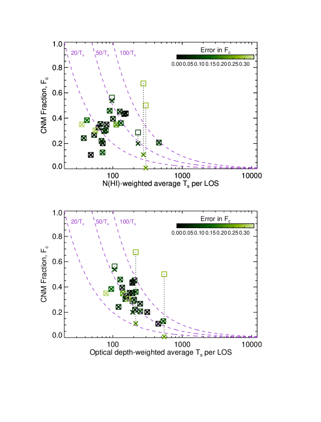
Figure 9: (Top) The CNM fraction as a function of the column density weighted $T_{s}$ along each line of sight for our observations (crosses). Propagated uncertainties, shown as a color bar, are just from the fitting of Gaussian components and do not include any systematic uncertainties inherent to the temperature derivation method. Crosses show the CNM fraction calculated when components with $T_{s}<200$ K are considered as the CNM, while squares show the $T_{s}<350$ K cut. The difference is very small and essentially only three sources have significantly changed their fraction. (Bottom) The CNM fraction as a function of the optical-depth weighted average $T_{s}$ (calculated using equation 15 in Kim et al. 2014), calculated using the optical depth and $T_{exp}$ profiles without Gaussian fitting. Again, squares show that the temperature cut does not affect a majority of our sources.

5 Comparison of CO and HI absorption spectra

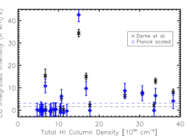
Figure 10: (Left) CO integrated intensity as a function of the total HI column density (CNM+WNM) in the direction of our 26 radio continuum sources. CO data from Dame et al. (2001) are shown in black for directions covered in this survey; the black dashed line shows the median 1-$\sigma$ uncertainty. CO data from Planck (Planck Collaboration et al., 2013) are shown in blue for all 26 sources after smoothing and regridding the CO integrated image to 8.4^′ resolution to match Dame et al.; the dashed blue lines shows the median 1-$\sigma$ uncertainty. To match Planck and Dame et al. values a constant scaling factor of 1.37 had to be applied to Planck data. (Right) CO integrated intensity plotted as a function of $A_{V}$ from Planck.

To compare HI absorption with CO we use data from two surveys: the CO (1-0) emission data from the CfA survey at 8.4’ resolution (Dame at al. 2001), and the integrated CO intensity ($W_{CO}$) from Planck (Planck Collaboration et al., 2013) smoothed and regridded to match the CfA’s angular resolution and pixel size. We extract CO spectra from Dame et al. and show $W_{CO}$ in Figure 10 (left) as black data points. The Dame et al. observed area covers 14 out of 26 sources. The dashed black line in this figure shows the median 1-$\sigma$ uncertainty on $W_{CO}$ calculated from the line-free channels. The results from Planck are shown in Figure 10 (left and right) in blue, as well as their median 1-$\sigma$ uncertainty. We noticed that Dame et al.’s integrated intensity is systematically higher relative to the Planck data. A median scaling of 1.37 was applied on the Planck data to roughly match Dame et al. observations.

Figure 10 shows that 8 out of 26 sources have a clearly detected CO emission that is above 1-$\sigma$ uncertainty in both Dame at al. and Planck data. Almost all detections have the total HI column density $>10^{21}$ cm^-2. Their CNM fraction ranges from 20% to 55%. While HI absorption is detected in the case of all sources, 18 sources were not detected in CO. Most non-detections pile up at $N(HI)<10^{21}$ cm^-2 and likely probe diffuse HI regions. As shown in Figure 10 (right) where we use the Planck data for $E(B-V)\times 3.19$ as a measure of $A_{V}$ ($R_{V}=3.19$ was measured for Perseus star BD+31^∘643 by (Snow et al., 1994)), most non-detections have $A_{V}<1$. Lee et al. (2014) showed that in Perseus $A_{V}\sim$1 mag is a necessary condition for the existence (shielding against photodissociation) of CO. Considering all this, most CO non-detections probe diffuse ($A_{V}<1$ mag) regions without necessary shielding for CO formation.

However, there are 3 CO non-detections with $N(HI)=$10-35 $\times 10^{20}$ cm^-2, which probe regions with $A_{V}\sim 1$ mag and therefore likely contain $H_{2}$, while CO could be just forming and still be underabundant. Considering that we detect HI absorption with large column density, yet no CO emission, these three positions are excellent candidates for probing the CO-dark gas which contains $H_{2}$ but not CO. Interestingly, CO is detected both at lower and higher total HI column density relative to these non-detection, at $\mathrel{\hbox{\hbox to0.0pt{\hbox{\lower 4.0pt\hbox{$\sim$}}\hss}\hbox{$<$}}}10^{21}$ and $>3\times 10^{21}$ cm^-2. The three sources are: 3C132, 3C093.1, and B20411+34. As shown in Figure 2, their HI absorption spectra have only components around 0 km/s suggesting that a contamination from non-Perseus HI clouds can not be the reason for HI absorption detections without CO emission.

We now compare closely the kinematics of CO (from Dame et al.) and HI absorption of 8 sources with detected CO which have $A_{V}\mathrel{\hbox{\hbox to0.0pt{\hbox{\lower 4.0pt\hbox{$\sim$}}\hss}\hbox{$>$}}}1$ mag (Figure 11). One of the eight sources, 3C092, is particularly interesting as it is located right behind the main body of Perseus, this source has the highest integrated CO intensity ($>30$ K km s^-1) and the CNM fraction of $\sim 0.4$. As shown in the figure, in most cases CO and HI absorption agree well in terms of velocity range and profile shapes, although there is a large diversity among sources. This suggests that HI in absorption appears to trace not just cloud envelopes but also central regions. In three cases (3C092, 3C108 and 4C+25.14) CO emission and HI absorption cover the same velocity range. In the case of 3C131, 3C133 and 4C+27.14, while the strongest HI absorption agrees well with the CO emission peak, a weaker secondary component is seen at a velocity of 0 km/s which is not detected in CO, possibly due to low sensitivity. Only for two sources, 4C+30.04 and 4C+33.10 there is significant difference in that the HI absorption profile is broader than CO emission and a CO peak is found in the middle of the HI absorption profile.

We show in Figure 11 the corresponding spin temperature and the CNM column density of the HI component that is the closest in velocity to the CO peak. The spin temperature ranges from 30 to 80 K, and the CNM column density of the component closest to CO ranges from 0.8 to 8 $\times 10^{20}$ cm^-2, which corresponds to the higher portion of the CNM column density measured for the whole population of CNM components in this study. On the other hand, the remaining CNM column density along these lines of sight ranges from $\sim 3\times 10^{20}$ to $13\times 10^{20}$ cm^-2. All sources except 4C+25+14 have the total HI column density $>10^{21}$ cm^-2 ($A_{V}\mathrel{\hbox{\hbox to0.0pt{\hbox{\lower 4.0pt\hbox{$\sim$}}\hss}\hbox{$>$}}}1$ mag), suggesting conditions suitable for formation of CO (and H₂).

This generally good spectral agreement we find between HI absorption and CO emission contrasts results from studies of the diffuse molecular gas ($A_{V}<1$ mag), e.g. Liszt & Lucas (1996); Liszt & Pety (2012), where commonly HI absorption is more extended in velocity relative to CO emission, and especially it was noticed that CO emission tends to avoid the deepest HI absorption (in other words, CO was associated only with weaker HI absorption features). This is usually explained as the deepest HI absorption arising mainly from the CO-free cloud envelopes, while CO tracing the central regions. The eight directions we investigate here all trace regions with $A_{V}\mathrel{\hbox{\hbox to0.0pt{\hbox{\lower 4.0pt\hbox{$\sim$}}\hss}\hbox{$>$}}}1$ and are therefore likely probing equilibrium chemistry relative to $A_{V}<1$ likely largely non-equilibrium dominated regions.

It is generally expected that the CO-dark gas is found in uniform envelopes surrounding CO-bright molecular clouds (Wolfire et al., 2010). Numerical simulations by Smith et al. (2014) support this idea but show that CO-dark H₂ may be asymmetric and not necessarily trace the outlines of CO-bright clouds. Fukui et al. (2014a) proposed that the CO-dark gas could be dominated by the optically thick HI. In addition, considering that envelopes are likely to have small velocity offsets relative to the CO-bright cloud regions, we would expect to see kinematically more extended HI absorption profiles around CO peaks. However, in eight directions where we have both HI absorption and CO emission spectra we generally find good agreement between the two. This suggests that in these directions HI absorption traces largely the central cloud regions where CO is bright, and to a smaller degree only the CO-dark cloud envelope. Of 26 directions there are only 3 cases with strong HI absorption and the total $N(HI)>10^{21}$ cm^-2, but without CO emission.

Another interesting result from our study is that cold HI with high HI column density is clearly present deep inside CO-bright GMCs, suggesting that its importance for GMC evolution, and star formation, may be more significant than previously thought. The origin of cold HI deep inside GMCs, and its morphology (e.g. filamentary flows vs clumps vs diffuse distribution throughout GMCs) are not well understood. The cold HI could be brought deep into the clouds via circulation of neutral gas from outer regions due to turbulence (Hennebelle & Inutsuka, 2006), or could be a photodissociation product of H₂. Tighter grids of HI absorption sources across and around GMCs are greatly needed to map out the distribution of cold HI and distinguish between various formation mechanisms.

6 Summary and Future Work

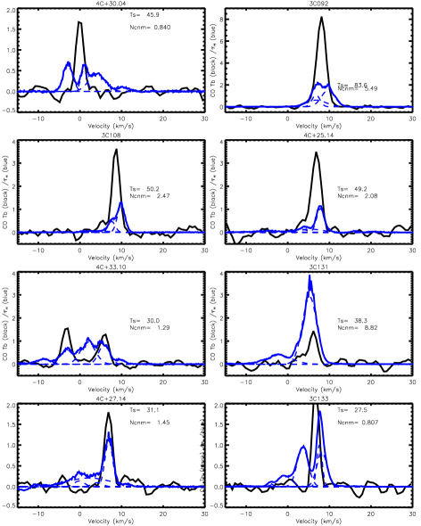
Figure 11: Comparison of CO emission (from Dame et al.) shown in black and HI absorption shown in blue. Each HI absorption profile has several Gaussian components shown as dashed lines. For each panel, properties of the HI absorption component that is closest in velocity to CO emission are listed in the top right corner: the corresponding spin temperature in K, the corresponding CNM HI column density in $10^{20}$ cm^-2, and the CNM fraction calculated for the whole line of sight.

To investigate properties of cold HI in and around Perseus molecular cloud, and especially to investigate the role of cold HI in the shielding of H₂ (Paper II), we have obtained and detected HI absorption in the direction of 26 background radio continuum sources. Using the corresponding HI emission spectra, and by employing a Gaussian decomposition of HI emission/absorption pairs, we have performed radiative transfer calculations to estimate $T_{s}$ and $\tau(v)$ for 107 individual Gaussian components. This method represents the most direct way of measuring spin temperature and optical depth.

The peak optical depth of individual Gaussian components ranges from $\sim 0.01$ to a few, with the median value of 0.16. The spin temperature ranges from 10 to 725 K, and peaks at 50 K. The median values of the CNM and WNM column densities for individual components are $6\times 10^{19}$ cm^-2 and $1.5\times 10^{20}$ cm^-2, respectively. All properties of individual components for Perseus are in excellent agreement with those of HT03, who observed 66 random lines of sight at $|b|>10^{\circ}$. This suggests that individual cold HI components have similar properties between a focused field around a GMC and an average ISM field.

However, when all CNM and WNM components are summed along each line of sight, we find a significant difference relative to an average ISM field. The Perseus region has a higher fraction of absorbing HI and a higher total HI column density relative to an average ISM field, suggesting environmental differences. This result is the first observational evidence that the CNM fraction in/around GMCs is likely higher than what is found in an average ISM field. Interestingly, the median CNM and WNM HI column density along the line of sight are roughly similar around Perseus, $4.6\times 10^{20}$ cm^-2 vs $5.8\times 10^{20}$ cm^-2, while in the case of HT03 the WNM column density was twice higher than the CNM column density.

Our results for both the optical depth and spin temperature are in stark contrast to Fukui et al. (2014) who used Planck data and assumed that all of dust grains cooler than 22 K are mixed with the optically thick HI, suggesting that the amount of cold HI could be significant and even enough to explain all (or most) of the CO-dark gas. For 85% of their sky coverage they estimated $T_{s}=20-40$ K and $\tau_{max}>0.5$. Considering all our Gaussian components, we find such high $\tau_{max}$ only occasionally, with only 20% of components having $\tau_{max}>0.5$. Considering whole optical depth profiles, 54% of directions have $\tau_{max}>0.5$. Also, only $\sim 15$% of lines of sight have a column density weighted average spin temperature lower than 40 K. We suspect that Fukui et al. results are caused by the non ability to distinguish different gas components along the line of sight, as well as by assigning all of the cooler dust to HI without allowing for contribution of the molecular gas (bright or dark).

The mean spin temperature appears uniform over the radius of 10 to 120 pc from the rough center of Perseus. Obtaining a tighter grid of HI absorption sources, and especially sampling better the inner 10 pc, in the future will be important to probe a potential radial increase in $T_{s}$ away from the cloud center as suggested by Andersson et al. (1992).

While the CNM fraction is on average higher around Perseus relative to a random ISM field, surprisingly it rarely exceeds 50%. Even directions with the lowest $T_{s}<200$ K clearly show the CNM fraction of $<50$%. It is highly encouraging to see that recent numerical simulations by Kim et al. (2014) produce the CNM fractions reasonably close to observations, $40-70$%, and also predict that the CNM fraction is inversely proportional to the optical-depth weighted average $T_{s}$, which is in excellent agreement with observations. Further inclusion of interstellar chemistry, and the HI-to-H₂ conversion, will likely fine-tune the simulated fractions and bring them even closer to observations. Our results suggest that even directions that probe deep inside molecular clouds do not have high CNM fractions (e.g. $>50$%). This could result from extended WNM envelopes of GMCs, and/or significant mixing of CNM and WNM throughout GMCs caused by interstellar turbulence or accretion flows. While the low CNM fraction in/around GMCs requires further theoretical work, at high column densities the HI lines are likely to become saturated and therefore poorly trace the densest and coldest regions of GMCs. It is therefore also important to observationally test usefulness of additional tracers of neutral gas inside GMCs, e.g. CI and CII.

Finally, we have compared HI absorption with CO emission for our 26 directions and found that 8/26 have detected CO. Out of the remaining 18, 15 directions probe diffuse regions with $A_{V}<1$ mag and likely do not have enough shielding for CO formation. Only 3/26 directions have $N(HI)>10^{21}$ cm^-2 ($A_{V}\mathrel{\hbox{\hbox to0.0pt{\hbox{\lower 4.0pt\hbox{$\sim$}}\hss}\hbox{$>$}}}1$ mag), and therefore probe conditions suitable for CO formation, yet have no detected CO emission. These directions therefore likely contain molecular gas but not CO and are representative of so called CO-dark gas. Eight directions with detected CO have $N(HI)>10^{21}$ cm^-2, $A_{V}>1$ mag, and good kinematic agreement between HI absorption and CO emission spectra. All of this suggests that these lines of sight probe largely central CO-bright regions, confirming the existence of cold HI deep inside GMCs. However, future observations of a tighter grid of background sources are necessary to map out the distribution of cold HI around GMCs and its origin.

Source	TB	VLSR	$\Delta$V	$\tau$	Ts	Tk,max	N(HI)20	$F$ or $O$
	(K)	(km s-1)	(km s-1)		(K)	(K)	(cm-2)
	(1)	(2)	(3)	(4)	(5)	(6)	(7)	(8)
3C067	1.88 $\pm$ 0.06	-25.8 $\pm$ 0.1	4.71 $\pm$ 0.18	0.0057	331.	835	0.17	1.0
3C067	1.95 $\pm$ 0.00	-11.6 $\pm$ 0.4	41.30 $\pm$ 0.64	0.0045	438.	2077	1.27	0.0
3C067	5.34	-5.8 $\pm$ 0.1	4.81 $\pm$ 0.18	0.10 $\pm$ 0.002	69.10 $\pm$ 8.88	325	0.62	2
3C067	21.02 $\pm$ 0.35	-2.3 $\pm$ 0.2	9.75 $\pm$ 0.17	0.0169	1254.	861	3.99	0.5
3C067	23.05	-0.3 $\pm$ 0.0	2.14 $\pm$ 0.04	0.41 $\pm$ 0.008	42.88 $\pm$ 8.28	607	0.74	0
3C067	17.71	1.2 $\pm$ 0.1	5.99 $\pm$ 0.13	0.19 $\pm$ 0.005	89.34 $\pm$ 14.82	489	1.94	1
3C067	3.41 $\pm$ 0.19	8.3 $\pm$ 0.2	6.28 $\pm$ 0.31	0.0005	6748.	485	0.41	0.0
3C068.2	1.24 $\pm$ 0.04	-19.8 $\pm$ 1.4	30.94 $\pm$ 2.61	0.0089	141.	20919	0.55	0.0
3C068.2	5.09	-6.2 $\pm$ 0.0	2.58 $\pm$ 0.07	0.27 $\pm$ 0.000	19.75 $\pm$ 8.88	144	0.27	0
3C068.2	-0.09	-3.0 $\pm$ 0.1	2.63 $\pm$ 0.24	0.09 $\pm$ 0.004	4.11 $\pm$ 8.28	151	0.02	3
3C068.2	20.81 $\pm$ 1.16	-2.7 $\pm$ 0.1	10.42 $\pm$ 0.25	0.0147	1422.	2370	4.22	0.0
3C068.2	31.03	1.3 $\pm$ 0.0	2.04 $\pm$ 0.05	0.90 $\pm$ 0.040	43.82 $\pm$ 14.82	91	1.57	2
3C068.2	16.32	3.1 $\pm$ 0.6	3.88 $\pm$ 0.62	0.11 $\pm$ 0.017	140.94 $\pm$ 5.04	328	1.15	1
3C068.2	3.44 $\pm$ 0.67	5.6 $\pm$ 2.1	15.15 $\pm$ 1.97	0.0194	179.	5017	0.96	1.0
3C092	1.01 $\pm$ 0.06	-53.1 $\pm$ 0.3	8.43 $\pm$ 0.67	0.0117	86.	119698	0.12	0.0
3C092	1.32 $\pm$ 0.04	-18.6 $\pm$ 0.9	74.01 $\pm$ 2.51	0.0059	224.	3173	1.18	0.0
3C092	3.45 $\pm$ 0.06	-4.9 $\pm$ 0.2	12.05 $\pm$ 0.48	0.0031	1118.	1661	0.81	0.0
3C092	6.36	6.8 $\pm$ 0.0	2.22 $\pm$ 0.06	1.08 $\pm$ 0.040	26.89 $\pm$ 8.28	151	1.26	2
3C092	6.36	6.9 $\pm$ 0.5	5.56 $\pm$ 0.35	0.61 $\pm$ 0.114	49.09 $\pm$ 8.88	144	3.23	1
3C092	49.81 $\pm$ 0.62	7.3 $\pm$ 0.0	8.72 $\pm$ 0.03	0.0025	19811.	328	8.46	1.0
3C092	4.39	9.7 $\pm$ 0.1	3.82 $\pm$ 0.12	1.50 $\pm$ 0.158	23.70 $\pm$ 14.82	91	2.65	0
3C093.1	1.86 $\pm$ 0.10	-21.2 $\pm$ 0.2	9.89 $\pm$ 0.69	0.0048	386.	1240	0.36	0.0
3C093.1	4.37 $\pm$ 0.07	-13.1 $\pm$ 0.3	47.01 $\pm$ 0.74	0.0016	2702.	328	3.60	0.0
3C093.1	36.62	6.2 $\pm$ 0.0	1.62 $\pm$ 0.09	0.41 $\pm$ 0.031	44.35 $\pm$ 8.28	151	0.57	0
3C093.1	33.75 $\pm$ 0.59	7.2 $\pm$ 0.0	7.53 $\pm$ 0.06	0.0031	11047.	48303	4.95	0.0
3C093.1	35.18	7.7 $\pm$ 0.0	4.45 $\pm$ 0.04	1.19 $\pm$ 0.043	45.36 $\pm$ 8.88	144	4.67	2
3C093.1	35.58	8.8 $\pm$ 0.0	1.36 $\pm$ 0.03	1.30 $\pm$ 0.036	23.35 $\pm$ 14.82	91	0.80	1
3C108	1.91 $\pm$ 0.05	-24.1 $\pm$ 0.9	29.33 $\pm$ 1.70	0.0045	425.	18806	0.92	0.0
3C108	1.55	-5.7 $\pm$ 0.5	4.73 $\pm$ 1.19	0.01 $\pm$ 0.002	64.12 $\pm$ 8.88	144	0.07	2
3C108	5.21 $\pm$ 0.18	-0.7 $\pm$ 0.1	4.69 $\pm$ 0.14	0.0066	792.	481	0.48	1.0
3C108	12.88	4.0 $\pm$ 0.3	7.52 $\pm$ 0.69	0.06 $\pm$ 0.002	194.98 $\pm$ 8.28	151	1.82	1
3C108	9.76 $\pm$ 0.19	6.7 $\pm$ 0.3	23.59 $\pm$ 0.31	0.0007	13061.	12158	4.42	0.0
3C108	29.59	7.6 $\pm$ 0.0	1.99 $\pm$ 0.05	0.47 $\pm$ 0.009	58.26 $\pm$ 14.82	91	1.07	0
3C108	37.55	9.9 $\pm$ 0.0	2.10 $\pm$ 0.02	1.20 $\pm$ 0.010	49.52 $\pm$ 5.04	328	2.44	3
3C131	16.27	-39.5 $\pm$ 0.0	3.74 $\pm$ 0.09	0.16 $\pm$ 0.003	100.90 $\pm$ 8.88	144	1.15	2
3C131	3.41	-34.0 $\pm$ 0.1	2.00 $\pm$ 0.33	0.03 $\pm$ 0.004	75.15 $\pm$ 8.28	151	0.09	3
3C131	2.28	-24.1 $\pm$ 0.2	3.37 $\pm$ 0.50	0.03 $\pm$ 0.003	114.31 $\pm$ 14.82	91	0.20	4
3C131	9.18 $\pm$ 0.15	-18.5 $\pm$ 0.3	53.41 $\pm$ 0.68	0.0079	1163.	745	8.82	0.0
3C131	4.62	-15.9 $\pm$ 0.3	6.76 $\pm$ 0.70	0.03 $\pm$ 0.002	227.36 $\pm$ 5.04	328	0.89	1
3C131	7.18 $\pm$ 0.26	-9.6 $\pm$ 0.1	4.94 $\pm$ 0.21	0.0036	2023.	745	0.69	0.0
3C131	46.95	-2.1 $\pm$ 0.0	7.31 $\pm$ 0.10	0.38 $\pm$ 0.003	145.62 $\pm$ 6.75	62335	7.99	0
3C131	46.76	5.2 $\pm$ 0.0	4.04 $\pm$ 0.02	2.93 $\pm$ 0.028	37.71 $\pm$ 6.26	534	8.68	5
3C131	45.98 $\pm$ 1.89	5.9 $\pm$ 0.0	5.84 $\pm$ 0.10	0.0234	1985.	745	5.23	0.0
3C131	6.36	11.9 $\pm$ 0.2	2.65 $\pm$ 0.54	0.02 $\pm$ 0.004	119.41 $\pm$ 6.19	745	0.13	6
3C132	6.16 $\pm$ 0.03	-15.4 $\pm$ 0.2	50.11 $\pm$ 0.37	0.0164	378.	54879	5.68	0.0
3C132	2.21	-2.3 $\pm$ 0.1	3.15 $\pm$ 0.28	0.05 $\pm$ 0.003	37.05 $\pm$ 8.88	144	0.12	0
3C132	11.81	2.0 $\pm$ 0.0	4.12 $\pm$ 0.07	0.34 $\pm$ 0.003	47.85 $\pm$ 8.28	151	1.29	2
3C132	38.49 $\pm$ 0.19	5.3 $\pm$ 0.0	14.52 $\pm$ 0.05	0.0068	5703.	4610	10.89	0.5
3C132	12.35	8.0 $\pm$ 0.0	2.54 $\pm$ 0.01	1.33 $\pm$ 0.008	35.41 $\pm$ 14.82	91	2.32	3
3C132	54.35 $\pm$ 2.87	8.4 $\pm$ 0.0	3.18 $\pm$ 0.02	0.0015	35172.	220	3.36	0.5
3C132	23.31	13.1 $\pm$ 0.0	5.24 $\pm$ 0.08	0.24 $\pm$ 0.002	109.33 $\pm$ 5.04	328	2.66	1
3C133	15.84	-29.8 $\pm$ 0.1	8.18 $\pm$ 0.17	0.05 $\pm$ 0.002	322.42 $\pm$ 8.88	1462	2.52	0
3C133	14.58	-27.7 $\pm$ 0.0	3.28 $\pm$ 0.11	0.07 $\pm$ 0.002	38.56 $\pm$ 8.28	234	0.17	3
3C133	10.16 $\pm$ 0.08	-16.8 $\pm$ 0.3	43.40 $\pm$ 0.44	0.0012	8199.	41156	8.26	0.5
3C133	3.20	-10.3 $\pm$ 0.1	5.98 $\pm$ 0.38	0.02 $\pm$ 0.001	219.63 $\pm$ 14.82	782	0.40	5
3C133	0.77	-4.3 $\pm$ 0.0	1.49 $\pm$ 0.05	0.08 $\pm$ 0.002	4.89 $\pm$ 5.04	48	0.01	6
3C133	5.98	-0.8 $\pm$ 0.0	3.96 $\pm$ 0.07	0.26 $\pm$ 0.001	12.37 $\pm$ 6.75	342	0.25	7
3C133	67.68 $\pm$ 0.54	2.5 $\pm$ 0.0	10.40 $\pm$ 0.05	0.0009	73191.	2362	13.71	0.0
3C133	42.16	3.6 $\pm$ 0.0	3.10 $\pm$ 0.02	0.95 $\pm$ 0.003	47.99 $\pm$ 6.26	210	2.77	8
3C133	48.15	7.6 $\pm$ 0.0	1.49 $\pm$ 0.02	1.01 $\pm$ 0.019	10.82 $\pm$ 36.16	48	0.32	2
3C133	49.11	8.2 $\pm$ 0.0	2.84 $\pm$ 0.02	0.83 $\pm$ 0.017	69.32 $\pm$ 6.19	176	3.19	4
3C133	11.35	11.9 $\pm$ 1.1	8.75 $\pm$ 1.56	0.02 $\pm$ 0.001	725.42 $\pm$ 17.67	1675	1.91	1
4C+25.14	1.86 $\pm$ 0.06	-23.5 $\pm$ 1.1	30.47 $\pm$ 1.82	0.0147	127.	20291	0.95	0.5
4C+25.14	0.14	-8.3 $\pm$ 4.5	16.30 $\pm$ 5.51	0.02 $\pm$ 0.006	12.84 $\pm$ 8.88	5802	0.09	2
4C+25.14	1.13	-4.7 $\pm$ 0.2	4.59 $\pm$ 0.88	0.04 $\pm$ 0.014	21.83 $\pm$ 8.28	462	0.09	0
4C+25.14	20.06	4.0 $\pm$ 0.1	1.82 $\pm$ 0.18	0.11 $\pm$ 0.011	41.54 $\pm$ 14.82	73	0.17	4
4C+25.14	19.63	5.3 $\pm$ 0.2	7.15 $\pm$ 0.38	0.14 $\pm$ 0.016	130.63 $\pm$ 5.04	1117	2.61	3
4C+25.14	8.95 $\pm$ 0.11	6.0 $\pm$ 0.3	27.53 $\pm$ 0.40	0.0022	4025.	16562	4.69	0.0
4C+25.14	36.35	7.8 $\pm$ 0.0	2.10 $\pm$ 0.03	1.03 $\pm$ 0.012	41.83 $\pm$ 6.75	96	1.77	1
4C+25.14	1.17	16.1 $\pm$ 0.1	1.76 $\pm$ 0.13	0.06 $\pm$ 0.004	15.94 $\pm$ 6.26	67	0.03	5
4C+25.14	0.90	20.9 $\pm$ 0.2	3.82 $\pm$ 0.41	0.03 $\pm$ 0.003	32.05 $\pm$ 6.19	318	0.07	6
4C+26.12	7.28	-7.0 $\pm$ 0.0	2.60 $\pm$ 0.05	0.16 $\pm$ 0.003	53.06 $\pm$ 8.88	5802	0.44	1
4C+26.12	1.45 $\pm$ 0.04	-6.1 $\pm$ 0.6	59.78 $\pm$ 1.92	0.0049	295.	1117	0.95	1.0
4C+26.12	6.59 $\pm$ 0.11	-3.9 $\pm$ 0.2	7.30 $\pm$ 0.26	0.0032	2088.	96	0.94	1.0
4C+26.12	4.61 $\pm$ 0.29	1.7 $\pm$ 0.1	4.46 $\pm$ 0.24	0.0008	6111.	67	0.40	0.0
4C+26.12	28.22	6.6 $\pm$ 0.1	8.95 $\pm$ 0.20	0.11 $\pm$ 0.003	182.48 $\pm$ 14.82	73	3.50	0
4C+26.12	28.39	6.7 $\pm$ 0.0	1.83 $\pm$ 0.04	0.30 $\pm$ 0.005	53.04 $\pm$ 8.28	462	0.56	2
4C+27.07	2.09 $\pm$ 0.02	-23.0 $\pm$ 0.0	24.44 $\pm$ 0.27	0.0124	169.	73	0.86	1.0
4C+27.07	8.35	-5.2 $\pm$ 0.1	3.67 $\pm$ 0.16	0.10 $\pm$ 0.003	87.61 $\pm$ 8.88	5802	0.60	0
4C+27.07	16.85 $\pm$ 0.14	-1.7 $\pm$ 0.0	10.73 $\pm$ 0.05	0.0224	761.	96	3.52	0.0
4C+27.07	15.70	-0.3 $\pm$ 0.0	2.96 $\pm$ 0.05	0.27 $\pm$ 0.004	61.24 $\pm$ 8.28	462	0.94	1
4C+27.07	2.24 $\pm$ 0.12	3.1 $\pm$ 0.3	20.01 $\pm$ 0.32	0.0023	971.	1117	0.79	0.0
4C+27.14	-1.05	-41.5 $\pm$ 0.1	1.74 $\pm$ 0.18	0.08 $\pm$ 0.007	3.58 $\pm$ 8.88	66	0.01	4
4C+27.14	13.09	-35.2 $\pm$ 0.0	2.49 $\pm$ 0.11	0.29 $\pm$ 0.012	34.00 $\pm$ 8.28	135	0.47	5
4C+27.14	14.70 $\pm$ 0.24	-34.1 $\pm$ 0.1	20.31 $\pm$ 0.25	0.0172	864.	9019	5.80	0.0
4C+27.14	8.28	-31.2 $\pm$ 0.3	7.65 $\pm$ 0.43	0.14 $\pm$ 0.005	65.97 $\pm$ 5.04	1278	1.33	7
4C+27.14	6.28	-28.9 $\pm$ 0.0	1.19 $\pm$ 0.07	0.23 $\pm$ 0.011	13.99 $\pm$ 14.82	30	0.07	6
4C+27.14	3.20	-20.7 $\pm$ 0.2	3.89 $\pm$ 0.42	0.05 $\pm$ 0.004	85.24 $\pm$ 6.75	330	0.32	8
4C+27.14	12.75 $\pm$ 0.41	-12.9 $\pm$ 0.1	8.42 $\pm$ 0.27	0.0052	2478.	1548	2.09	0.0
4C+27.14	34.04	-0.1 $\pm$ 0.1	2.84 $\pm$ 0.31	0.14 $\pm$ 0.016	45.07 $\pm$ 6.26	176	0.35	1
4C+27.14	33.23	2.2 $\pm$ 0.1	12.26 $\pm$ 0.46	0.21 $\pm$ 0.020	161.68 $\pm$ 36.16	3287	8.06	0
4C+27.14	19.03 $\pm$ 1.55	2.8 $\pm$ 0.3	19.60 $\pm$ 0.50	0.0145	1320.	8396	7.23	0.0
4C+27.14	28.87	4.2 $\pm$ 0.3	2.86 $\pm$ 0.74	0.10 $\pm$ 0.019	13.99 $\pm$ 6.19	178	0.07	3
4C+27.14	38.30 $\pm$ 2.39	5.0 $\pm$ 0.0	5.66 $\pm$ 0.14	0.0044	8820.	700	4.23	0.0
4C+27.14	40.88	6.9 $\pm$ 0.0	2.18 $\pm$ 0.05	1.10 $\pm$ 0.022	12.82 $\pm$ 17.67	103	0.60	2
4C+28.06	2.07 $\pm$ 0.05	-6.9 $\pm$ 0.3	39.13 $\pm$ 0.60	0.0021	984.	330	1.23	1.0
4C+28.06	4.83	-6.8 $\pm$ 0.1	4.80 $\pm$ 0.17	0.07 $\pm$ 0.002	73.35 $\pm$ 8.88	66	0.51	2
4C+28.06	16.89 $\pm$ 0.12	0.3 $\pm$ 0.0	11.72 $\pm$ 0.11	0.0058	2937.	176	3.85	1.0
4C+28.06	14.32	1.5 $\pm$ 0.0	5.31 $\pm$ 0.07	0.28 $\pm$ 0.004	69.60 $\pm$ 8.28	135	2.02	3
4C+28.06	12.98	3.3 $\pm$ 0.0	1.85 $\pm$ 0.06	0.24 $\pm$ 0.007	27.27 $\pm$ 14.82	30	0.24	1
4C+28.06	1.16	7.8 $\pm$ 0.1	1.70 $\pm$ 0.23	0.03 $\pm$ 0.003	36.98 $\pm$ 5.04	1278	0.04	0
4C+28.07	0.73 $\pm$ 0.02	-16.5 $\pm$ 0.7	56.11 $\pm$ 1.46	0.0034	212.	178	0.35	0.0
4C+28.07	20.10	-6.3 $\pm$ 0.0	2.36 $\pm$ 0.10	0.15 $\pm$ 0.009	58.15 $\pm$ 8.28	135	0.40	1
4C+28.07	19.34	-5.7 $\pm$ 0.1	6.19 $\pm$ 0.42	0.08 $\pm$ 0.009	169.27 $\pm$ 8.88	66	1.71	2
4C+28.07	11.90	0.7 $\pm$ 0.1	3.02 $\pm$ 0.08	0.57 $\pm$ 0.019	16.40 $\pm$ 14.82	30	0.55	4
4C+28.07	9.04 $\pm$ 0.28	1.2 $\pm$ 0.1	16.08 $\pm$ 0.13	0.0019	4685.	176	2.79	0.0
4C+28.07	31.30 $\pm$ 0.71	1.4 $\pm$ 0.0	4.65 $\pm$ 0.02	0.0045	6920.	3287	2.83	0.0
4C+28.07	6.65	3.2 $\pm$ 0.2	2.94 $\pm$ 0.25	0.19 $\pm$ 0.026	39.45 $\pm$ 5.04	1278	0.42	0
4C+28.07	0.99	6.7 $\pm$ 1.4	6.25 $\pm$ 1.93	0.02 $\pm$ 0.003	139.49 $\pm$ 6.75	330	0.28	3
4C+29.05	1.57 $\pm$ 0.03	-11.4 $\pm$ 0.2	43.60 $\pm$ 0.47	0.0160	99.	330	0.96	1.0
4C+29.05	0.67	-8.0 $\pm$ 0.1	2.20 $\pm$ 0.31	0.03 $\pm$ 0.003	32.58 $\pm$ 8.88	66	0.04	0
4C+29.05	6.13 $\pm$ 0.08	-4.4 $\pm$ 0.1	16.62 $\pm$ 0.13	0.0082	752.	1278	1.97	1.0
4C+29.05	6.28	-1.3 $\pm$ 0.0	3.93 $\pm$ 0.08	0.14 $\pm$ 0.003	49.20 $\pm$ 8.28	135	0.54	1
4C+29.05	7.87 $\pm$ 0.10	-0.4 $\pm$ 0.0	7.94 $\pm$ 0.07	0.0017	4770.	30	1.22	0.0
4C+30.04	1.30 $\pm$ 0.04	-4.8 $\pm$ 0.7	42.10 $\pm$ 1.04	0.0191	68.	38738	0.74	1.0
4C+30.04	23.10	-2.9 $\pm$ 0.0	2.62 $\pm$ 0.02	0.67 $\pm$ 0.007	45.83 $\pm$ 8.88	149	1.57	1
4C+30.04	19.23	1.0 $\pm$ 0.0	1.83 $\pm$ 0.05	0.51 $\pm$ 0.013	40.71 $\pm$ 8.28	73	0.74	3
4C+30.04	35.95 $\pm$ 0.22	2.3 $\pm$ 0.0	10.46 $\pm$ 0.03	0.0109	3326.	2391	7.33	0.0
4C+30.04	7.00	4.1 $\pm$ 0.1	4.61 $\pm$ 0.12	0.43 $\pm$ 0.004	15.64 $\pm$ 14.82	465	0.60	2
4C+30.04	0.09	10.4 $\pm$ 0.1	3.16 $\pm$ 0.15	0.10 $\pm$ 0.004	1.99 $\pm$ 5.04	217	0.01	0
4C+30.04	4.26 $\pm$ 0.11	13.7 $\pm$ 0.3	13.23 $\pm$ 0.50	0.0161	267.	3822	1.06	0.0
4C+33.10	4.68	-52.8 $\pm$ 0.1	2.36 $\pm$ 0.13	0.12 $\pm$ 0.006	33.86 $\pm$ 8.88	149	0.19	4
4C+33.10	12.70 $\pm$ 0.39	-46.2 $\pm$ 0.2	17.41 $\pm$ 0.43	0.0037	3394.	1017	4.29	0.0
4C+33.10	10.10	-44.8 $\pm$ 0.0	3.06 $\pm$ 0.09	0.20 $\pm$ 0.006	52.19 $\pm$ 8.28	73	0.62	5
4C+33.10	12.34 $\pm$ 1.36	-43.2 $\pm$ 0.3	4.50 $\pm$ 0.29	0.0039	3180.	1017	1.08	0.0
4C+33.10	5.44 $\pm$ 0.30	-30.6 $\pm$ 0.2	6.82 $\pm$ 0.54	0.0026	2081.	1017	0.72	0.0
4C+33.10	3.88	-16.1 $\pm$ 0.1	2.77 $\pm$ 0.25	0.07 $\pm$ 0.005	45.43 $\pm$ 14.82	465	0.17	6
4C+33.10	4.41	-8.8 $\pm$ 0.1	4.27 $\pm$ 0.17	0.21 $\pm$ 0.005	19.31 $\pm$ 5.04	217	0.33	7
4C+33.10	34.42 $\pm$ 0.45	-6.8 $\pm$ 0.1	24.91 $\pm$ 0.23	0.0118	2933.	1017	16.62	0.0
4C+33.10	23.35	-3.2 $\pm$ 0.1	3.57 $\pm$ 0.12	0.62 $\pm$ 0.010	48.13 $\pm$ 6.75	443	2.07	0
4C+33.10	43.26	1.9 $\pm$ 0.1	4.21 $\pm$ 0.21	0.95 $\pm$ 0.012	69.69 $\pm$ 6.26	13556	5.43	1
4C+33.10	42.58	5.8 $\pm$ 0.1	3.03 $\pm$ 0.11	0.83 $\pm$ 0.028	70.14 $\pm$ 6.19	684	3.44	2
4C+33.10	26.72 $\pm$ 1.09	7.3 $\pm$ 0.2	5.59 $\pm$ 0.17	0.0116	2317.	1017	2.91	0.0
4C+33.10	7.53	9.7 $\pm$ 0.1	2.46 $\pm$ 0.14	0.19 $\pm$ 0.007	36.57 $\pm$ 36.16	6621	0.34	3
4C+34.07	2.00 $\pm$ 0.00	-22.7 $\pm$ 0.0	3.07 $\pm$ 0.10	0.0132	153.	3403	0.12	1.0
4C+34.07	1.70 $\pm$ 0.03	-9.1 $\pm$ 0.3	46.64 $\pm$ 0.63	0.0002	10602.	217	1.14	0.0
4C+34.07	20.20	-2.2 $\pm$ 0.0	1.84 $\pm$ 0.05	0.24 $\pm$ 0.007	21.05 $\pm$ 8.88	149	0.18	0
4C+34.07	20.62	-1.0 $\pm$ 0.0	5.63 $\pm$ 0.10	0.15 $\pm$ 0.009	140.20 $\pm$ 8.28	73	2.26	2
4C+34.07	7.21 $\pm$ 0.09	0.3 $\pm$ 0.0	12.48 $\pm$ 0.11	0.0086	845.	47549	1.75	0.0
4C+34.07	18.91	1.1 $\pm$ 0.0	1.79 $\pm$ 0.11	0.09 $\pm$ 0.006	63.79 $\pm$ 14.82	465	0.21	1
4C+34.09	2.30 $\pm$ 0.05	-10.2 $\pm$ 0.5	61.68 $\pm$ 1.46	0.0051	452.	217	2.18	0.0
4C+34.09	0.74	-8.0 $\pm$ 0.0	1.69 $\pm$ 0.03	0.22 $\pm$ 0.004	4.79 $\pm$ 8.88	149	0.03	2
4C+34.09	7.65 $\pm$ 0.12	-2.1 $\pm$ 0.1	8.36 $\pm$ 0.20	0.0017	4607.	83144	1.25	1.0
4C+34.09	35.09	1.1 $\pm$ 0.0	2.70 $\pm$ 0.06	0.24 $\pm$ 0.005	93.71 $\pm$ 8.28	73	1.19	0
4C+34.09	27.38	4.7 $\pm$ 0.1	9.80 $\pm$ 0.11	0.19 $\pm$ 0.002	157.27 $\pm$ 14.82	465	5.79	1
5C06.237	2.30 $\pm$ 0.05	-7.4 $\pm$ 0.3	40.50 $\pm$ 0.71	0.0031	750.	217	1.48	0.0
5C06.237	14.03	-1.3 $\pm$ 0.0	3.42 $\pm$ 0.07	0.40 $\pm$ 0.004	52.28 $\pm$ 8.88	149	1.40	1
5C06.237	14.48 $\pm$ 0.20	-0.5 $\pm$ 0.0	9.96 $\pm$ 0.10	0.0094	1545.	465	2.81	1.0
5C06.237	6.37	2.0 $\pm$ 0.1	2.18 $\pm$ 0.16	0.10 $\pm$ 0.006	62.11 $\pm$ 8.28	73	0.27	0
B20218+35	5.23 $\pm$ 0.03	-57.9 $\pm$ 0.0	14.08 $\pm$ 0.10	0.0112	471.	217	1.35	0.0
B20218+35	2.25 $\pm$ 0.03	-10.4 $\pm$ 0.2	45.22 $\pm$ 0.53	0.0026	881.	4332	1.54	0.0
B20218+35	3.89	-4.5 $\pm$ 0.2	2.77 $\pm$ 0.50	0.03 $\pm$ 0.011	116.48 $\pm$ 8.88	149	0.19	0
B20218+35	12.27 $\pm$ 0.36	-0.3 $\pm$ 0.0	10.40 $\pm$ 0.12	0.0028	4331.	44682	2.48	0.0
B20218+35	6.84	-0.3 $\pm$ 0.9	6.24 $\pm$ 2.03	0.04 $\pm$ 0.030	49.87 $\pm$ 14.82	465	0.26	1
B20218+35	8.44	0.7 $\pm$ 0.1	2.82 $\pm$ 0.34	0.11 $\pm$ 0.031	62.21 $\pm$ 8.28	73	0.38	2
B20326+27	1.33 $\pm$ 0.03	-12.7 $\pm$ 0.6	64.39 $\pm$ 1.51	0.0037	364.	217	0.96	1.0
B20326+27	19.44	0.4 $\pm$ 0.0	4.67 $\pm$ 0.07	0.30 $\pm$ 0.003	78.55 $\pm$ 8.88	149	2.12	0
B20326+27	19.93 $\pm$ 0.14	3.0 $\pm$ 0.0	13.20 $\pm$ 0.05	0.0184	1093.	465	5.12	0.5
B20326+27	23.00	6.7 $\pm$ 0.0	4.56 $\pm$ 0.06	0.34 $\pm$ 0.003	83.42 $\pm$ 8.28	73	2.49	1
B20400+25	1.97 $\pm$ 0.10	-48.0 $\pm$ 0.1	5.04 $\pm$ 0.32	0.0017	1189.	35507	0.18	0.0
B20400+25	1.91 $\pm$ 0.04	-27.4 $\pm$ 0.5	40.31 $\pm$ 1.29	0.0112	171.	217	1.38	1.0
B20400+25	17.65	5.0 $\pm$ 0.4	14.63 $\pm$ 0.63	0.03 $\pm$ 0.002	607.24 $\pm$ 8.28	73	4.58	0
B20400+25	33.18	7.2 $\pm$ 0.0	2.17 $\pm$ 0.04	0.31 $\pm$ 0.007	67.41 $\pm$ 14.82	465	0.88	2
B20400+25	23.82	8.6 $\pm$ 0.1	4.79 $\pm$ 0.10	0.16 $\pm$ 0.006	54.35 $\pm$ 8.88	149	0.80	1
B20400+25	1.38 $\pm$ 0.06	19.9 $\pm$ 0.3	13.70 $\pm$ 0.88	0.0033	422.	555	0.30	0.0
B20411+34	2.34 $\pm$ 0.27	-28.4 $\pm$ 4.6	48.16 $\pm$ 5.23	0.0136	174.	50696	1.90	0.0
B20411+34	1.44	-14.4 $\pm$ 0.3	3.86 $\pm$ 0.66	0.02 $\pm$ 0.004	14.83 $\pm$ 8.88	325	0.03	3
B20411+34	11.85 $\pm$ 0.59	-4.8 $\pm$ 0.2	27.39 $\pm$ 0.65	0.0133	899.	16401	6.23	0.0
B20411+34	3.88	-3.3 $\pm$ 0.2	5.27 $\pm$ 0.35	0.07 $\pm$ 0.003	106.09 $\pm$ 8.28	607	0.74	2
B20411+34	18.58 $\pm$ 0.70	4.1 $\pm$ 0.2	8.50 $\pm$ 0.26	0.0080	2322.	1577	3.07	0.0
B20411+34	35.65	5.1 $\pm$ 0.1	4.73 $\pm$ 0.20	0.90 $\pm$ 0.128	39.17 $\pm$ 14.82	489	3.27	1
B20411+34	25.16	8.5 $\pm$ 1.5	6.18 $\pm$ 1.27	0.18 $\pm$ 0.073	68.77 $\pm$ 5.04	835	1.53	0
NV0157+28	2.80 $\pm$ 0.02	-13.6 $\pm$ 0.1	40.62 $\pm$ 0.25	0.0083	340.	446	1.91	0.0
NV0157+28	2.40 $\pm$ 0.04	-10.4 $\pm$ 0.0	4.52 $\pm$ 0.09	0.0022	1098.	489	0.21	0.0
NV0157+28	14.89	-2.7 $\pm$ 0.1	9.76 $\pm$ 0.18	0.05 $\pm$ 0.001	302.10 $\pm$ 8.88	325	2.90	1
NV0157+28	13.69	-0.5 $\pm$ 0.0	1.96 $\pm$ 0.12	0.04 $\pm$ 0.002	25.80 $\pm$ 8.28	607	0.04	0
NV0157+28	3.80 $\pm$ 0.10	2.7 $\pm$ 0.2	10.56 $\pm$ 0.26	0.0041	932.	835	0.77	1.0
NV0232+34	2.69 $\pm$ 0.03	-6.5 $\pm$ 0.1	39.32 $\pm$ 0.37	0.0110	245.	33787	1.68	0.0
NV0232+34	20.16	-1.9 $\pm$ 0.1	2.04 $\pm$ 0.16	0.13 $\pm$ 0.010	43.04 $\pm$ 8.28	607	0.22	0
NV0232+34	22.52	-0.1 $\pm$ 0.2	8.49 $\pm$ 0.71	0.06 $\pm$ 0.014	321.07 $\pm$ 8.88	325	3.10	2
NV0232+34	22.90	0.4 $\pm$ 0.0	1.82 $\pm$ 0.09	0.20 $\pm$ 0.012	37.38 $\pm$ 14.82	489	0.27	3
NV0232+34	14.61	3.0 $\pm$ 0.1	2.11 $\pm$ 0.19	0.09 $\pm$ 0.008	30.54 $\pm$ 5.04	835	0.11	1

References

- Andersson et al. (1992) Andersson, B.-G., Roger, R. S., & Wannier, P. G. 1992, A&A, 260, 355
- Andersson & Wannier (1993) Andersson, B.-G. & Wannier, P. G. 1993, ApJ, 402, 585
- Audit & Hennebelle (2005) Audit, E. & Hennebelle, P. 2005, A&A, 433, 1
- Bigiel et al. (2008) Bigiel, F., Leroy, A., Walter, F., et al. 2008, AJ, 136, 2846
- Blitz et al. (2007) Blitz, L., Fukui, Y., Kawamura, A., et al. 2007, Protostars and Planets V, 81
- Blitz & Rosolowsky (2004) Blitz, L. & Rosolowsky, E. 2004, ApJ, 612, L29
- Chieze & Pineau Des Forets (1989) Chieze, J. P. & Pineau Des Forets, G. 1989, A&A, 221, 89
- Clark et al. (2012) Clark, P. C., Glover, S. C. O., Klessen, R. S., & Bonnell, I. A. 2012, MNRAS, 424, 2599
- Condon et al. (1998) Condon, J. J., Cotton, W. D., Greisen, E. W., et al. 1998, AJ, 115, 1693
- Dame et al. (2001) Dame, T. M., Hartmann, D., & Thaddeus, P. 2001, ApJ, 547, 792
- Dickey et al. (2009) Dickey, J. M., Strasser, S., Gaensler, B. M., et al. 2009, ApJ, 693, 1250
- Elmegreen (1993) Elmegreen, B. G. 1993, ApJ, 411, 170
- Fukui & Kawamura (2010) Fukui, Y. & Kawamura, A. 2010, ARA&A, 48, 547
- Fukui et al. (2009) Fukui, Y., Kawamura, A., Wong, T., et al. 2009, ApJ, 705, 144
- Fukui et al. (2014a) Fukui, Y., Okamoto, R., Yamamoto, H., et al. 2014a, astro-ph/1401.7398, submitted to ApJ
- Fukui et al. (2014b) Fukui, Y., Torii, K., Onishi, T., et al. 2014b, astro-ph/1403.0999, submitted to ApJ
- Gibson et al. (2000) Gibson, S. J., Taylor, A. R., Higgs, L. A., & Dewdney, P. E. 2000, ApJ, 540, 851
- Goldbaum et al. (2011) Goldbaum, N. J., Krumholz, M. R., Matzner, C. D., & McKee, C. F. 2011, ApJ, 738, 101
- Goldsmith & Li (2005) Goldsmith, P. F. & Li, D. 2005, ApJ, 622, 938
- González Hernández et al. (2009) González Hernández, J. I., Iglesias-Groth, S., Rebolo, R., et al. 2009, ApJ, 706, 866
- Gooch (1996) Gooch, R. 1996, Astronomical Data Analysis Software and Systems V, 101, 80
- Goodman & Heiles (1994) Goodman, A. A. & Heiles, C. 1994, ApJ, 424, 208
- Haslam et al. (1982) Haslam, C. G. T., Stoffel, H., Salter, C. J., & Wilson, W. E. 1982, A&AS, 47, 1
- Heiles & Troland (2003a) Heiles, C. & Troland, T. H. 2003a, ApJS, 145, 329
- Heiles & Troland (2003b) —. 2003b, ApJ, 586, 1067
- Heitsch et al. (2005) Heitsch, F., Burkert, A., Hartmann, L. W., Slyz, A. D., & Devriendt, J. E. G. 2005, ApJ, 633, L113
- Hennebelle & Inutsuka (2006) Hennebelle, P. & Inutsuka, S.-i. 2006, ApJ, 647, 404
- Herbig & Jones (1983) Herbig, G. H. & Jones, B. F. 1983, AJ, 88, 1040
- Kalberla et al. (2005) Kalberla, P. M. W., Dedes, L., Arnal, E. M., et al. 2005, in ASP Conf. Ser. 331: Extra-Planar Gas, 81
- Kim et al. (2014) Kim, C.-G., Ostriker, E. C., & Kim, W.-T. 2014, ApJ, 786, 64
- Kim & Ostriker (2006) Kim, W.-T. & Ostriker, E. C. 2006, ApJ, 646, 213
- Knapp (1974) Knapp, G. R. 1974, AJ, 79, 527
- Krumholz et al. (2009) Krumholz, M. R., McKee, C. F., & Tumlinson, J. 2009, ApJ, 693, 216
- Lada et al. (2010) Lada, C. J., Lombardi, M., & Alves, J. F. 2010, ApJ, 724, 687
- Lee et al. (2012) Lee, M.-Y., Stanimirović, S., Douglas, K. A., et al. 2012, ApJ, 748, 75
- Li & Goldsmith (2003) Li, D. & Goldsmith, P. F. 2003, ApJ, 585, 823
- Liljestrom & Mattila (1988) Liljestrom, T. & Mattila, K. 1988, A&A, 196, 243
- Liszt & Lucas (1996) Liszt, H. & Lucas, R. 1996, A&A, 314, 917
- Liszt & Pety (2012) Liszt, H. S. & Pety, J. 2012, A&A, 541, A58
- McKee & Ostriker (1977) McKee, C. F. & Ostriker, J. P. 1977, ApJ, 218, 148
- Miville-Deschênes & Lagache (2005) Miville-Deschênes, M.-A. & Lagache, G. 2005, ApJS, 157, 302
- Peek et al. (2011) Peek, J. E. G., Heiles, C., Douglas, K. A., et al. 2011, ApJS, 194, 20
- Pineda et al. (2008) Pineda, J. E., Caselli, P., & Goodman, A. A. 2008, ApJ, 679, 481
- Planck Collaboration et al. (2013) Planck Collaboration, Ade, P. A. R., Aghanim, N., et al. 2013, astro-ph/1303.5073, submitted to A&A
- Ridge et al. (2006) Ridge, N. A., Di Francesco, J., Kirk, H., 2006, AJ, 131, 2921
- Sancisi et al. (1974) Sancisi, R., Goss, W. M., Anderson, C., Johansson, L. E. B., & Winnberg, A. 1974, A&A, 35, 445
- Schruba et al. (2011) Schruba, A., Leroy, A. K., Walter, F., et al. 2011, AJ, 142, 37
- Shetty et al. (2014) Shetty, R., Kelly, B. C., Rahman, N., et al. 2014, MNRAS, 437, L61
- Shu (1973) Shu, F. H. 1973, American Scientist, 61, 524
- Smith et al. (2014) Smith, R. J., Glover, S. C. O., Clark, P. C., Klessen, R. S., & Springel, V. 2014, MNRAS, 441, 1628
- Snow et al. (1994) Snow, T. P., Hanson, M. M., Seab, G. C., & Saken, J. M. 1994, ApJ, 420, 632
- Spitzer & Jenkins (1975) Spitzer, Jr., L. & Jenkins, E. B. 1975, ARA&A, 13, 133
- Stanimirović & Heiles (2005) Stanimirović, S. & Heiles, C. 2005, ApJ, 631, 371
- Stanimirović et al. (2007) Stanimirović, S., Heiles, C., & Kanekar, N. 2007, in Astronomical Society of the Pacific Conference Series, Vol. 365, SINS - Small Ionized and Neutral Structures in the Diffuse Interstellar Medium, ed. M. Haverkorn & W. M. Goss, 22
- Stanimirović et al. (2006) Stanimirović, S., Putman, M., Heiles, C., et al. 2006, ApJ, 653, 1210
- Strasser et al. (2007) Strasser, S. T., Dickey, J. M., Taylor, A. R., et al. 2007, AJ, 134, 2252
- Wannier et al. (1991) Wannier, P. G., Lichten, S. M., Andersson, B.-G., & Morris, M. 1991, ApJS, 75, 987
- Wannier et al. (1983) Wannier, P. G., Lichten, S. M., & Morris, M. 1983, ApJ, 268, 727
- Wolfire et al. (2010) Wolfire, M. G., Hollenbach, D., & McKee, C. F. 2010, ApJ, 716, 1191
- Wolfire et al. (2003) Wolfire, M. G., McKee, C. F., Hollenbach, D., & Tielens, A. G. G. M. 2003, ApJ, 587, 278
- Wong & Blitz (2002) Wong, T. & Blitz, L. 2002, ApJ, 569, 157