A New characterization and global regularity
of infinite energy solutions
to the homogeneous Boltzmann equation

Abstract.

The purpose of this paper is to introduce a new characterization of the characteristic functions for the study on the measure valued solution to the homogeneous Boltzmann equation so that it precisely captures the moment constraint in physics. This significantly improves the previous result by Cannone-Karch [CPAM 63(2010), 747-778] in the sense that the new characterization gives a complete description of infinite energy solutions for the Maxwellian cross section. In addition, the global in time smoothing effect of the infinite energy solution except for a single Dirac mass initial datum is justified as for the finite energy solution.

1. Introduction

Consider the spatially homogeneous Boltzmann equation,

(1.1) $$\partial_{t}f(t,v)=Q(f,f)(t,v),$$

where $f(t,v)$ is the density distribution of particles with velocity $v\in{{\mathbb{R}}}^{3}$ at time $t$. The most interesting and important part of this equation is the collision operator given on the right hand side that captures the change rates of the density distribution through elastic binary collisions:

$$Q(g,f)(v)=\int_{{{\mathbb{R}}}^{3}}\int_{\mathbb{S}^{2}}B\left({v-v_{*}},\sigma\right)\left\{g(v^{\prime}_{*})f(v^{\prime})-g(v_{*})f(v)\right\}d\sigma dv_{*}\,,$$

where for $\sigma\in\SS^{2}$

$$v^{\prime}=\frac{v+v_{*}}{2}+\frac{|v-v_{*}|}{2}\sigma,\,\,\,v^{\prime}_{*}=\frac{v+v_{*}}{2}-\frac{|v-v_{*}|}{2}\sigma,\,$$

that follow from the conservation of momentum and energy,

$$v^{\prime}+v_{*}^{\prime}=v+v_{*},\enskip|v^{\prime}|^{2}+|v_{*}^{\prime}|^{2}=|v|^{2}+|v_{*}|^{2}.$$

In this paper, we consider the Cauchy problem of (1.1) with initial datum

(1.2) $$f(0,v)=F_{0}\geq 0.$$

Motivated by some physical models, we assume that the non-negative cross section $B$ takes the form

$$B(|v-v_{*}|,\cos\theta)=\Phi(|v-v_{*}|)b(\cos\theta),\,\,\,\,\,\cos\theta=\frac{v-v_{*}}{|v-v_{*}|}\,\cdot\,\sigma\,,\,\,\,0\leq\theta\leq\frac{\pi}{2},$$

where

$$\Phi(|z|)=\Phi_{\gamma}(|z|)=|z|^{\gamma},\enskip\mbox{for some $\gamma>-3$},$$

(1.3) $$b(\cos\theta)\theta^{2+2s}\ \rightarrow K\ \ \mbox{when}\ \ \theta\rightarrow 0+,\enskip\mbox{for $0<s<1$ and $K>0$. }$$

Throughout this paper, we will only consider the case when

$$\gamma=0,\enskip 0<s<1\,,$$

which is called Maxwellian molecule type cross section, because the analysis relies on the simpler form of the equation after taking Fourier transform in $v$ by the Bobylev formula. As usual, the range of $\theta$ can be restricted to $[0,\pi/2]$, by replacing $b(\cos\theta)$ by its “symmetrized” version

$$[b(\cos\theta)+b(\cos(\pi-\theta))]{\bf 1}_{0\leq\theta\leq\pi/2}.$$

It is now well known that the angular singularity in the cross section leads to the gain of regularity in the solution. The purpose of this paper is to show that this still holds for measure valued solutions. Moreover, we improve the previous work on existence theory by Cannonne-Karch [2] because we introduce a new classification of the characteristic functions so that the moment constraints can be precisely captured in the Fourier space.

We start with the following a slightly general assumption on the cross section

(1.4) $$\exists\alpha_{0}\in(0,2]\enskip\mbox{ such that}\enskip(\sin\theta/2)^{\alpha_{0}}b(\cos\theta)\sin\theta\in L^{1}((0,\pi/2]),$$

which is fulfilled for $b$ with (1.3) if $2s<\alpha_{0}$.

Denote by $P_{\alpha}({{\mathbb{R}}}^{d})$, $0\leq\alpha\leq 2$ the probability measures $F$ on ${{\mathbb{R}}}^{d}$, $d\geq 1$, such that

$$\int_{{{\mathbb{R}}}^{d}}|v|^{\alpha}dF(v)<\infty,\,$$

and moreover when $\alpha\geq 1$ , it requires that

(1.5) $$\int_{{{\mathbb{R}}}^{d}}v_{j}dF(v)=0,\enskip j=1,\cdots d\,.$$

Following Cannone-Karch [2], the Fourier transform of a probability measure $F\in P_{0}({{\mathbb{R}}}^{d})$ called a characteristic function is defined by by

$$\varphi(\xi)=\hat{f}(\xi)={\mathcal{F}}(F)(\xi)=\int_{{{\mathbb{R}}}^{d}}e^{-iv\cdot\xi}dF(v).$$

Put ${\mathcal{K}}={\mathcal{F}}(P_{0}({{\mathbb{R}}}^{d}))$. Inspired by a series of works by Toscani and co-authors[3, 4, 8], Cannone-Karch defined a subspace ${\mathcal{K}}^{\alpha}$ for $\alpha\geq 0$ as follows:

(1.6) $${\mathcal{K}}^{\alpha}=\{\varphi\in{\mathcal{K}}\,;\,\|\varphi-1\|_{\alpha}<\infty\}\,,$$

where

(1.7) $$\|\varphi-1\|_{\alpha}=\sup_{\xi\in{{\mathbb{R}}}^{d}}\frac{|\varphi(\xi)-1|}{|\xi|^{\alpha}}.$$

The space ${\mathcal{K}}^{\alpha}$ endowed with the distance

(1.8) $$\|\varphi-\tilde{\varphi}\|_{\alpha}=\sup_{\xi\in{{\mathbb{R}}}^{d}}\frac{|\varphi(\xi)-\tilde{\varphi}(\xi)|}{|\xi|^{\alpha}}$$

is a complete metric space (see Proposition 3.10 of [2]). It follows that ${\mathcal{K}}^{\alpha}=\{1\}$ for all $\alpha>2$ and the following embeddings (Lemma 3.12 of [2]) hold

$$\{1\}\subset{\mathcal{K}}^{\alpha}\subset{\mathcal{K}}^{\beta}\subset{\mathcal{K}}^{0}={\mathcal{K}}\enskip\enskip\mbox{for all $2\geq\alpha\geq\beta\geq 0$}\,\,.$$

With this classification on the characteristic functions, the global existence of solution in ${\mathcal{K}}^{\alpha}$ was studied in [2](see also [5]). However, even though the inclusion ${\mathcal{F}}(P_{\alpha}({{\mathbb{R}}}^{d}))\subset{\mathcal{K}}^{\alpha}$ holds (see Lemma 3.15 of [2]), the space ${\mathcal{K}}^{\alpha}$ is strictly bigger than ${\mathcal{F}}(P_{\alpha}({{\mathbb{R}}}^{d}))$ for $\alpha\in(0,2)$, in other word, ${\mathcal{F}}^{-1}({\mathcal{K}}^{\alpha})\supsetneq P^{\alpha}({{\mathbb{R}}}^{d})$. Indeed, it is shown (see Remark 3.16 of [2]) that the function $\varphi_{\alpha}(\xi)=e^{-|\xi|^{\alpha}}$, with $\alpha\in(0,2)$, belongs to ${\mathcal{K}}^{\alpha}$ but $p_{\alpha}(v)={\mathcal{F}}^{-1}(\varphi_{\alpha})(v)$, the density of $\alpha-$stable symmetric Lévy process, is not contained in $P_{\alpha}({{\mathbb{R}}}^{d})$. Hence, the solution obtained in the function space ${\mathcal{K}}^{\alpha}$ does not represent the moment properties in physics even when it is assumed initially.

In order to fill this gap, one main purpose of this paper is to introduce a new classification on the characteristic functions as follows. Set

(1.9) $${\mathcal{M}}^{\alpha}=\{\varphi\in{\mathcal{K}}\,;\,\|\varphi-1\|_{{\mathcal{M}}^{\alpha}}<\infty\}\,,\enskip\alpha\in(0,2)\,,$$

where

(1.10) $$\|\varphi-1\|_{{\mathcal{M}}^{\alpha}}=\int_{{{\mathbb{R}}}^{d}}\frac{|\varphi(\xi)-1|}{|\xi|^{d+\alpha}}d\xi\,.$$

For $\varphi,\tilde{\varphi}\in{\mathcal{M}}^{\alpha}$, put

$$\|\varphi-\tilde{\varphi}\|_{{\mathcal{M}}^{\alpha}}=\int_{{{\mathbb{R}}}^{d}}\frac{|\varphi(\xi)-\tilde{\varphi}(\xi)|}{|\xi|^{d+\alpha}}d\xi\,,$$

and, for any $\beta\in(0,\alpha]$, we introduce the distance

(1.11) $${dis}_{\alpha,\beta}(\varphi,\tilde{\varphi})=\|\varphi-\tilde{\varphi}\|_{{\mathcal{M}}^{\alpha}}+\|\varphi-\tilde{\varphi}\|_{\beta}\,.$$

With the above notations, the first main result in this paper can be stated as follows.

Theorem 1.1.

If $0<\beta\leq\alpha<2$, then the space ${\mathcal{M}}^{\alpha}$ is a complete metric space endowed with the distance $dis_{\alpha,\beta}(\varphi,\tilde{\varphi})$. If $\beta,\beta^{\prime}$ are in $(0,\alpha]$, both distances $dis_{\alpha,\beta}(\cdot,\cdot)$ and $dis_{\alpha,\beta^{\prime}}(\cdot,\cdot)$ are equivalent in the following sense:

(1.12) $$\forall\varepsilon>0 \exists\delta>0 dis_{\alpha,\beta}(\varphi,\varphi_{0})<\delta \Rightarrow dis_{\alpha,\beta^{\prime}}(\varphi,\varphi_{0})<\varepsilon$$, s.t. .

Moreover, we have

(1.13) $${\mathcal{K}}^{\beta}\subset{\mathcal{M}}^{\alpha}\enskip\mbox{if $\alpha<\beta$ and $\alpha\in(0,2)$,}$$

(1.14) $${\mathcal{M}}^{\alpha}\subset{\mathcal{F}}(P_{\alpha}({{\mathbb{R}}}^{d}))\,\big{(}\,\,\subsetneq{\mathcal{K}}^{\alpha}\,\,\big{)}\enskip\mbox{for}\enskip\alpha\in(0,2)\,,$$

(1.15) $${\mathcal{M}}^{\alpha}={\mathcal{F}}(P_{\alpha}({{\mathbb{R}}}^{d}))\,,\enskip\mbox{furthermore if $\alpha\neq 1$ },$$

and the fact that $\displaystyle\lim_{n\rightarrow\infty}dis_{\alpha,\beta}(\varphi_{n},\varphi)=0$, for $\varphi_{n},\varphi\in{\mathcal{M}}^{\alpha}$, implies

(1.16) $$\lim_{n\rightarrow\infty}\int\psi(v)dF_{n}(v)=\int\psi(v)dF(v)\mbox{ for any $\psi\in C({{\mathbb{R}}}^{d})$}$$

      satisfying the growth condition $$|\psi(v)|\lesssim\langle v\rangle^{\alpha}$$,

where $F_{n}={\mathcal{F}}^{-1}(\varphi_{n}),F={\mathcal{F}}^{-1}(\varphi)\in P_{\alpha}({{\mathbb{R}}}^{d})$.

Remark 1.2.

If $F\in P_{1}({{\mathbb{R}}}^{d})$ satisfies $\int_{{{\mathbb{R}}}^{d}}\langle v\rangle\log\langle v\rangle dF_{0}(v)<\infty,$ then we have ${\mathcal{F}}(F)\in{\mathcal{M}}^{1}$ (see Proposition 2.1 below).

Remark 1.3.

The weak convergence (1.16) is equivalent to the one given by the Wasserstein distance (see Theorem 7.12 of [11]).

Thanks to the new characterization of $P_{\alpha}$ by its exact Fourier image ${\mathcal{M}}^{\alpha}$, we can improve results, given in [2, 5, 7], concerning the existence and the smoothing effect of measure valued solutions to the Cauchy problem for the spatially homogeneous Boltzmann equation of Maxwellian molecule type cross section without angular cutoff that will be stated as follows.

Theorem 1.4.

Assume that $b$ satisfies (1.4) for some $\alpha_{0}\in(0,2)$ and let $\alpha\in[\alpha_{0},2),\alpha\neq 1$. If $F_{0}\in P_{\alpha}({{\mathbb{R}}}^{3})$, then there exists a unique measure valued solution $F_{t}\in C([0,\infty),P_{\alpha}({{\mathbb{R}}}^{3}))$ to the Cauchy problem (1.1)-(1.2), where the continuity with respect to $t$ is according to the topology deduced in the sense of (1.16).

Remark 1.5.

When $F_{0}\in P_{1}({{\mathbb{R}}}^{3})$, the result is slightly weaker, that is, for any $T>0$ there exists a constant $C_{T}>0$ such that

(1.17) $$\sup_{0\leq t\leq T}\int_{{{\mathbb{R}}}^{3}}\langle v\rangle dF_{t}(v)\leq C_{T}.$$

Moreover, if $F_{0}\in P_{1}({{\mathbb{R}}}^{3})$ satisfies $\int_{{{\mathbb{R}}}^{3}}\langle v\rangle\log\langle v\rangle dF_{0}(v)<\infty,$ then the solution $F_{t}\in C([0,\infty),P_{1}({{\mathbb{R}}}^{3}))$.

The proof of the above theorem is given in the Fourier space. In fact, by letting $\varphi(t,\xi)=\int_{{{\mathbb{R}}}^{3}}e^{-iv\cdot\xi}dF_{t}(v)$ and $\varphi_{0}={\mathcal{F}}(F_{0})$, it follows from the Bobylev formula that the Cauchy problem (1.1)-(1.2) is reduced to

(1.18) $$\left\{\begin{array}[]{l}\displaystyle\partial_{t}\varphi(t,\xi)=\int_{\SS^{2}}b\left(\frac{\xi\cdot\sigma}{|\xi|}\right)\Big{(}\varphi(t,\xi^{+})\varphi(t,\xi^{-})-\varphi(t,\xi)\varphi(t,0)\Big{)}d\sigma,\\ \\ \displaystyle\varphi(0,\xi)=\varphi_{0}(\xi),\enskip\mbox{where}\enskip\displaystyle\xi^{\pm}=\frac{\xi}{2}\pm\frac{|\xi|}{2}\sigma\,.\end{array}\right.$$

By Theorem 1.1, to prove Theorem 1.4 it suffices to show

Theorem 1.6.

Assume that $b$ satisfies (1.4) for some $\alpha_{0}\in(0,2)$ and let $\alpha\in[\alpha_{0},2)$. If the initial datum $\varphi_{0}$ belongs to ${\mathcal{M}}^{\alpha}$, then there exists a unique classical solution $\varphi(t,\xi)\in C([0,\infty),{\mathcal{M}}^{\alpha})$ to the Cauchy problem (1.18) such that

(1.19) $$dis_{\alpha,\alpha}(\varphi(t,\cdot),\varphi(s,\cdot))\lesssim|t-s|e^{\lambda_{\alpha}\max\{t,s\}}dis_{\alpha,\alpha}(\varphi_{0},1)\,.$$

Here

(1.20) $$\lambda_{\alpha}=2\pi\int_{0}^{\pi/2}b\left(\cos\theta\right)\left(\cos^{\alpha}\frac{\theta}{2}+\sin^{\alpha}\frac{\theta}{2}-1\right)\sin\theta d\theta>0\,.$$

Furthermore, if $\varphi(t,\xi),\tilde{\varphi}(t,\xi)\in C([0,\infty),{\mathcal{M}}^{\alpha})$ are two solutions to the Cauchy problem (1.18) with initial data $\varphi_{0},\tilde{\varphi}_{0}\in{\mathcal{M}}^{\alpha}$, respectively, then for any $t>0$, the following two stability estimates hold

(1.21) $$||\varphi(t)-\tilde{\varphi}(t)||_{{\mathcal{M}}^{\alpha}}\leq e^{\lambda_{\alpha}t}||\varphi_{0}-\tilde{\varphi}_{0}||_{{\mathcal{M}}^{\alpha}}\,,$$

(1.22) $$||\varphi(t)-\tilde{\varphi}(t)||_{\alpha}\leq e^{\lambda_{\alpha}t}||\varphi_{0}-\tilde{\varphi}_{0}||_{\alpha}\,.$$

Remark 1.7.

Since $\varphi_{0},\tilde{\varphi}_{0}\in{\mathcal{M}}^{\alpha}\subset{\mathcal{K}}^{\alpha}$, the stability estimate (1.22) is nothing but (13) of [5].

As in [7], set $\tilde{P}_{\alpha}({{\mathbb{R}}}^{3})={\mathcal{F}}^{-1}({\mathcal{K}}^{\alpha})$ endowed with the distance (1.8). We are now ready to state the global in time smoothing effect for infinite energy solutions to the Cauchy problem (1.1)-(1.2), which is an improvement of Theorem 1.3 of [7], where the time global smoothing effect for finite energy solutions and a short time smoothing effect for infinite energy solutions were proved.

Theorem 1.8.

Let $b(\cos\theta)$ satisfy (1.3) with $0<s<1$ and let $\alpha\in(2s,2]$. If $F_{0}\in\tilde{P}_{\alpha}({{\mathbb{R}}}^{3})$ is not a single Dirac mass and $f(t,v)$ is a unique solution in $C([0,\infty),\tilde{P}_{\alpha}({{\mathbb{R}}}^{3}))$ to the Cauchy problem (1.1)-(1.2), then $f(t,\cdot)$ belongs to $H^{\infty}({{\mathbb{R}}}^{3})$ for any $t>0$. If $F_{0}\in P_{\alpha}({{\mathbb{R}}}^{3})$ then $f(t,\cdot)$ belongs to $L^{1}_{\alpha}({{\mathbb{R}}}^{3})\cap H^{\infty}({{\mathbb{R}}}^{3})$ for any $t>0$, and moreover when $\alpha\neq 1$, we have $f(t,v)\in C((0,\infty),L^{1}_{\alpha}({{\mathbb{R}}}^{3})\cap H^{\infty}({{\mathbb{R}}}^{3}))$.

The rest of the paper will be organized as follows. In the following section, we will prove the needed estimates for the new classification ${\mathcal{M}}^{\alpha}$ of ${\mathcal{K}}$. The existence of measure valued solution in the function space ${\mathcal{M}}^{\alpha}$ will be discussed in Section 3 and the global in time smoothing effect of the solution will be proved in the last section.

2. Characterization of $P_{\alpha}$

In this section, we will prove the estimates on ${\mathcal{M}}^{\alpha}$ stated in Theorem 1.1. For this, we first prove the following two propositions.

Proposition 2.1.

If $0<\alpha<2$, $\alpha\neq 1$ and if $F\in P_{\alpha}({{\mathbb{R}}}^{d})$, then there exists a $C>0$ depending only on $d$ and $\alpha$ such that for $\varphi={\mathcal{F}}(F)$ we have

(2.1) $$\|\varphi-1\|_{{\mathcal{M}}^{\alpha}}=\int_{{{\mathbb{R}}}^{d}}\frac{|\varphi(\xi)-1|}{|\xi|^{d+\alpha}}d\xi\leq C\int_{{{\mathbb{R}}}^{d}}\langle v\rangle^{\alpha}dF(v)\,.$$

When $\alpha=1$, we have $\varphi\in{\mathcal{M}}^{\alpha}$ if $F\in P_{1}({{\mathbb{R}}}^{d})$ satisfies

(2.2) $$\int\langle v\rangle\log\langle v\rangle dF(v)<\infty\,.$$

Proof.

Note

$$\varphi(\xi)-1 =\int_{{{\mathbb{R}}}^{d}}(e^{-iv\cdot\xi}-1)dF(v)$$

$$=\int_{{{\mathbb{R}}}^{d}}\Big{(}e^{-iv\cdot\xi}-\sum_{\ell\leq[\alpha]}\frac{1}{\ell!}(-iv\cdot\xi)^{\ell}\Big{)}dF(v),$$

because of (1.5) when $\alpha\geq 1$. By the polar coordinate $\xi=\rho\omega$ ($\rho>0,\omega\in\SS^{d-1}$), we have

$$\Big{|}e^{-iv\cdot\xi}-\sum_{\ell\leq[\alpha]}\frac{1}{\ell!}(-iv\cdot\xi)^{\ell}\Big{|}\lesssim\min\big{\{}(|v|\rho)^{[\alpha]+1}\,,\,\big{(}1+(|v|\rho)^{[\alpha]}\big{)}\big{\}}\,,$$

so that

$$\int_{\{|\xi|\leq 1\}}\frac{|1-\varphi(\xi)|}{|\xi|^{d+\alpha}}d\xi\leq\int_{{{\mathbb{R}}}^{d}}\Big{(}\int_{{\{|\xi|\leq 1\}}}\Big{|}e^{-iv\cdot\xi}-\sum_{\ell\leq[\alpha]}\frac{1}{\ell!}(-iv\cdot\xi)^{\ell}\Big{|}\frac{d\xi}{|\xi|^{d+\alpha}}\Big{)}dF(v)$$

$$\lesssim\int_{{{\mathbb{R}}}_{v}^{d}}\Big{(}\int_{0}^{\langle v\rangle^{-1}}\frac{(|v|\rho)^{[\alpha]+1}}{\rho^{1+\alpha}}d\rho+\int_{\langle v\rangle^{-1}}^{1}\frac{1+(|v|\rho)^{[\alpha]}}{\rho^{1+\alpha}}d\rho\Big{)}dF(v)$$

$$\lesssim\int_{{{\mathbb{R}}}_{v}^{d}}\langle v\rangle^{\alpha}dF(v)\enskip\mbox{if $\alpha\neq 1$},\enskip\lesssim\int_{{{\mathbb{R}}}_{v}^{d}}\langle v\rangle\log\langle v\rangle dF(v)\enskip\mbox{if $\alpha=1$}.$$

Consequently, we have the estimate (2.1) because $\int_{\{|\xi|>1\}}\frac{1}{|\xi|^{d+\alpha}}d\xi<\infty$. ∎

Conversely, we have

Proposition 2.2.

Let $\alpha\in(0,2)$ and let ${\mathcal{M}}^{\alpha}$ be a subspace of ${\mathcal{K}}={\mathcal{F}}(P_{0}({{\mathbb{R}}}^{d}))$ defined by (1.9). Then we have the inclusion (1.14). Furthermore, for $M\in[1,\infty]$, if we put

(2.3) $$c_{\alpha,d,M}=\int_{\{|\zeta|\leq M\}}\frac{\sin^{2}(\mathbf{e}_{1}\cdot\zeta/2)}{|\zeta|^{d+\alpha}}d\zeta>0,$$

and if $F={\mathcal{F}}^{-1}(\varphi)$ for $\varphi\in{\mathcal{M}}^{\alpha}$, then for any $R>0$ we have

(2.4) $$\int_{\{|v|\geq R\}}|v|^{\alpha}dF(v)\leq\frac{1}{2c_{\alpha,d,1}}\int_{\{|\xi|\leq 1/R\}}\frac{|1-\varphi(\xi)|}{|\xi|^{d+\alpha}}d\xi.$$

Moreover,

(2.5) $$\int_{{{\mathbb{R}}}^{d}}|v|^{\alpha}dF(v)\leq\frac{1}{2c_{\alpha,d,\infty}}\int_{{{\mathbb{R}}}^{d}}\frac{|1-\varphi(\xi)|}{|\xi|^{d+\alpha}}d\xi\,.$$

Proof.

Since $|\varphi(\xi)|\leq\varphi(0)=1$, we have

$$\int_{\{|\xi|\leq M/R\}}\frac{|1-\varphi(\xi)|}{|\xi|^{d+\alpha}}d\xi \geq\int_{\{|\xi|\leq M/R\}}\frac{\mbox{Re}~{}(1-\varphi(\xi))}{|\xi|^{d+\alpha}}d\xi$$

$$=\int_{{{\mathbb{R}}}_{v}^{d}}\Big{(}\int_{\{|\xi|\leq M/R\}}\frac{2\sin^{2}(v\cdot\xi/2)}{|\xi|^{d+\alpha}}d\xi\Big{)}dF(v).$$

By the change of variable $|v|\xi=\zeta$ and by using the invariance of the rotation, we have

$$\int_{\{|\xi|\leq M/R\}}\frac{\sin^{2}(v\cdot\xi/2)}{|\xi|^{d+\alpha}}d\xi =|v|^{\alpha}\int_{\{|\zeta|\leq M|v|/R\}}\frac{\sin^{2}(\mathbf{e}_{1}\cdot\zeta/2)}{|\zeta|^{d+\alpha}}d\zeta$$

$$\geq|v|^{\alpha}{\bf 1}_{\{|v|\geq R\}}c_{\alpha,d,M}\,,$$

which yields (2.4), with the choice of $M=1$. By letting $M\rightarrow\infty$ and $R\rightarrow 0$, we obtain (2.5). In order to complete the proof of (1.14), it remains to show (1.5) when $\alpha\geq 1$. Suppose that

$$\exists\varphi\in{\mathcal{M}}^{\alpha}\enskip s.t.\enskip a:=\int vdF(v)\neq 0\,,\enskip F={\mathcal{F}}^{-1}(\varphi).$$

Since $F(\cdot+a)$ belongs to $P_{\alpha}({{\mathbb{R}}}^{d})$ and satisfies (1.5), it follows from Proposition 2.1 that its Fourier transform

$$\varphi_{a}(\xi)=\int e^{-iv\cdot\xi}dF(v+a)=e^{ia\cdot\xi}\varphi(\xi)$$

belongs to ${\mathcal{M}}^{\alpha}$, that is,

$$\infty>\int_{{{\mathbb{R}}}^{d}}\frac{|1-e^{ia\cdot\xi}\varphi(\xi)|}{|\xi|^{d+\alpha}}d\xi=\int_{{{\mathbb{R}}}^{d}}\frac{|(e^{-ia\cdot\xi}-1)+(1-\varphi(\xi))|}{|\xi|^{d+\alpha}}d\xi\,.$$

Since $\varphi\in{\mathcal{M}}^{\alpha}$, we obtain $\int_{{{\mathbb{R}}}^{d}}\frac{|e^{-ia\cdot\xi}-1|}{|\xi|^{d+\alpha}}d\xi<\infty$, which contradicts $a\neq 0$. In fact, by the rotation, we can assume $a=(0,\cdots,0,|a|)$ and hence

$$\infty>\int_{{{\mathbb{R}}}^{d}}\frac{|e^{-ia\cdot\xi}-1|}{|\xi|^{d+\alpha}}d\xi\geq|\SS^{d-2}|\int_{0}^{\pi/2}\Big{(}\int_{0}^{1/|a|}\frac{\sin(\rho|a|\cos\theta)}{\rho^{1+\alpha}}d\rho\Big{)}d\theta\,.$$

∎

We are now ready to prove Theorem 1.1.

Proof of Theorem 1.1.

Suppose that $\{\varphi_{n}\}_{n=1}^{\infty}\subset{\mathcal{M}}^{\alpha}$ satisfies

$$dis_{\alpha,\beta}(\varphi_{n},\varphi_{m})\rightarrow 0\enskip(n,m\rightarrow\infty)\enskip,\enskip 0<\beta\leq\alpha<2.$$

Since it follows from Proposition 3.10 of [2] that ${\mathcal{K}}^{\beta}$ is a complete metric space, we have the limit (pointwise convergence)

$$\varphi(\xi)=\lim_{n\rightarrow\infty}\varphi_{n}(\xi)\in{\mathcal{K}}^{\beta}\subset{\mathcal{K}}.$$

For any fixed $R>1$ we have

$$\int_{\{R^{-1}\leq|\xi|\leq R\}}\frac{|\varphi_{n}(\xi)-1|}{|\xi|^{d+\alpha}}d\xi\leq\sup_{n}\|\varphi_{n}-1\|_{{\mathcal{M}}^{\alpha}}<\infty.$$

Taking the limit with respect to $n$ and letting $R\rightarrow\infty$, we have $\varphi\in{\mathcal{M}}^{\alpha}$. Now it is easy to see that $dis_{\alpha,\beta}(\varphi_{n},\varphi)\rightarrow 0$.

To prove (1.13), we will show that there exists a $C_{\alpha,\beta,d}>0$ depending only on $\alpha,\beta,d$ such that

(2.6) $$\|\varphi-1\|_{{\mathcal{M}}^{\alpha}}\leq C_{\alpha,\beta,d}\|\varphi-1\|_{\beta}^{\alpha/\beta},\enskip\mbox{for $\varphi\in{\mathcal{K}}^{\beta}$\,.}$$

Since $|\varphi(\xi)|\leq\varphi(0)=1$, for $R>0$ we have

$$\|\varphi-1\|_{{\mathcal{M}}^{a}}\leq\int_{\{|\xi|>1/R\}}\frac{2}{|\xi|^{d+\alpha}}d\xi+\int_{\{|\xi|\leq 1/R\}}\frac{\|\varphi-1\|_{\beta}}{|\xi|^{d+\alpha-\beta}}d\xi\,,$$

which gives (2.6) by taking $R\sim\|\varphi-1\|_{\beta}^{1/\beta}$. By Proposition 2.2, we get (1.14), that is, ${\mathcal{M}}^{\alpha}\subset{\mathcal{F}}(P_{\alpha}({{\mathbb{R}}}^{d}))$. Since it follows from Lemma 3.15 of [2] that ${\mathcal{F}}(P_{\alpha}({{\mathbb{R}}}^{d}))\subset{\mathcal{K}}^{\alpha}$, we have ${\mathcal{M}}^{\alpha}\subset{\mathcal{K}}^{\alpha}$. More precisely, there exist $C_{1},C_{2}>0$ such that for $\varphi\in{\mathcal{M}}^{\alpha},\,F={\mathcal{F}}^{-1}(\varphi)$, we have

(2.7) $$\|\varphi-1\|_{\alpha}\leq C_{1}\int_{{{\mathbb{R}}}^{d}}|v|^{\alpha}dF(v)\leq C_{2}\|\varphi-1\|_{{\mathcal{M}}^{\alpha}}\,,$$

where the second inequality follows from (2.5).

We will now show (1.12). Let $\beta\in(0,\alpha)$ and suppose that $dis_{\alpha,\beta}(\varphi,\varphi_{0})<\delta$ for $\varphi,\varphi_{0}\in{\mathcal{M}}^{\alpha}$. Noting that

$$\frac{\varphi(\xi)-\varphi_{0}(\xi)}{|\xi|^{\alpha}}=\int_{{{\mathbb{R}}}^{d}}\frac{e^{-i\xi\cdot v}-1}{(|\xi||v|)^{\alpha}}|v|^{\alpha}\Big{(}dF(v)-dF_{0}(v)\Big{)},\enskip \alpha\in(0,1)$$ if ,

$$\frac{\varphi(\xi)-\varphi_{0}(\xi)}{|\xi|^{\alpha}}=\int_{{{\mathbb{R}}}^{d}}\frac{e^{-i\xi\cdot v}-1+i\xi\cdot v}{(|\xi||v|)^{\alpha}}|v|^{\alpha}\Big{(}dF(v)-dF_{0}(v)\Big{)},\enskip \alpha\in[1,2)$$ if ,

we have, for any $1<\tilde{R}<R$,

$$\sup_{|\xi|<R^{-1}}\frac{|\varphi(\xi)-\varphi_{0}(\xi)|}{|\xi|^{\alpha}} \leq\sup_{|\xi|<R^{-1}}\int_{\{|v|<\tilde{R}\}}\Big{(}|v||\xi|\Big{)}^{1+[\alpha]-\alpha}|v|^{\alpha}\Big{(}dF(v)+dF_{0}(v)\Big{)}$$

$$\quad+3\int_{\{|v|\geq\tilde{R}\}}|v|^{\alpha}\Big{(}dF(v)+dF_{0}(v)\Big{)}$$

$$=I_{1}(R,\tilde{R})+I_{2}(\tilde{R})\,.$$

It follows from (2.4) that

$$I_{2}(\tilde{R}) \leq\frac{3}{2c_{\alpha,d,1}}\int_{\{|\xi|\leq 1/{\tilde{R}}\}}\frac{|1-\varphi(\xi)|+|1-\varphi_{0}(\xi)|}{|\xi|^{d+\alpha}}d\xi$$

$$\leq\frac{3}{c_{\alpha,d,1}}\Big{(}\int_{\{|\xi|\leq 1/{\tilde{R}}\}}\frac{|1-\varphi_{0}(\xi)|}{|\xi|^{d+\alpha}}d\xi+\|\varphi-\varphi_{0}\|_{{\mathcal{M}}^{a}}\Big{)}.$$

Hence, for any $\varepsilon>0$ there exists a $\tilde{R}>1$ such that $I_{2}(\tilde{R})<\varepsilon+{3\delta}/{c_{\alpha,d,1}}$. If $\tilde{R}>1$ is fixed as above, then we have

$$I_{1}(R,\tilde{R})\leq 2\frac{\tilde{R}^{1+[\alpha]}}{R^{1+[\alpha]-\alpha}}\rightarrow 0\,,\enskip R\rightarrow\infty\,.$$

Consequently, for any $\varepsilon>0$ there exists $R>1$ such that

$$\sup_{|\xi|<R^{-1}}\frac{|\varphi(\xi)-\varphi_{0}(\xi)|}{|\xi|^{\alpha}}\leq 2\varepsilon+\frac{3\delta}{c_{\alpha,d,1}}.$$

On the other hand,

$$\sup_{|\xi|\geq R^{-1}}\frac{|\varphi(\xi)-\varphi_{0}(\xi)|}{|\xi|^{\alpha}}\leq R^{\alpha-\beta}\sup_{|\xi|\geq R^{-1}}\frac{|\varphi(\xi)-\varphi_{0}(\xi)|}{|\xi|^{\beta}}\leq R^{\alpha-\beta}\delta\,.$$

Thus, we obtain (1.12) with $\beta^{\prime}=\alpha$. Other cases are easier because for $\beta^{\prime}>0$,

$$\sup_{|\xi|\geq R}\frac{|\varphi(\xi)-\varphi_{0}(\xi)|}{|\xi|^{\beta^{\prime}}}\rightarrow 0\enskip(R\rightarrow\infty)\,.$$

The exact characterization formula (1.15), when $\alpha\neq 1$, is a direct consequence of (2.1) and (2.4). Suppose that, for $F_{n},F\in P_{\alpha}({{\mathbb{R}}}^{d})$, we have

$$\varphi_{n}={\mathcal{F}}(F_{n}),\varphi={\mathcal{F}}(F)\in{\mathcal{M}}^{\alpha},\enskip\mbox{and}\enskip\displaystyle\lim_{n\rightarrow\infty}dis_{\alpha,\beta}(\varphi_{n},\varphi)=0\,.$$

Note that for $R>1$

$$\int_{\{|\xi|\leq 1/R\}}\frac{|1-\varphi_{n}(\xi)|}{|\xi|^{d+\alpha}}d\xi\leq\int_{\{|\xi|\leq 1/R\}}\frac{|1-\varphi(\xi)|}{|\xi|^{d+\alpha}}d\xi+\|\varphi_{n}-\varphi\|_{{\mathcal{M}}^{\alpha}}\,.$$

It follows from (2.4) that for any $\varepsilon>0$ there exist $R>1$ and $N\in{\mathbb{N}}$ such that

$$\int_{\{|v|\geq R\}}|v|^{\alpha}dF_{n}(v)+\int_{\{|v|\geq R\}}|v|^{\alpha}dF(v)<\varepsilon\,\enskip\mbox{if $n\geq N$}.$$

This shows (1.16) because $\varphi_{n}\rightarrow\varphi$ in ${\mathcal{S}}^{\prime}({{\mathbb{R}}}^{d})$ and so $F_{n}\rightarrow F$ in ${\mathcal{S}}^{\prime}({{\mathbb{R}}}^{d})$. And this completes the proof of the theorem. ∎

3. Proofs of Theorem 1.4 and Theorem 1.6

The main purpose of this section concerns with the existence of measure valued solutions in the new classification of the characteristic functions. We only need to prove Theorem 1.6 because Theorem 1.4 follows by using Theorem 1.1.

3.1. Existence under the cutoff assumption

As usual, the existence for non-cutoff cross section is based on the cutoff approximations. Hence, in this subsection, we assume that

(3.8) $$\gamma_{2}=\int_{\SS^{2}}b\Big{(}\frac{\xi\cdot\sigma}{|\xi|}\Big{)}d\sigma=2\pi\int_{0}^{\pi/2}b(\cos\theta)\sin\theta d\theta<\infty\,.$$

The existence and stability with cutoff cross section can be stated as follows.

Proposition 3.1.

Let $\alpha\in(0,2)$ and $b$ satisfy (3.8). For every initial datum $\varphi_{0}\in{\mathcal{M}}^{\alpha}$, there exists a unique classical solution to the Cauchy problem (1.18) satisfying $\varphi(t)\in C([0,\infty),{\mathcal{M}}^{\alpha})$. Furthermore, if $\varphi(t,\xi),\tilde{\varphi}(t,\xi)\in C([0,\infty),{\mathcal{M}}^{\alpha})$ are two solutions to the Cauchy problem (1.18) with initial data $\varphi_{0},\tilde{\varphi}_{0}\in{\mathcal{M}}^{\alpha}$, respectively, then for any $t>0$ we have

(3.9) $$||\varphi(t)-\tilde{\varphi}(t)||_{{\mathcal{M}}^{\alpha}}\leq e^{\lambda_{\alpha}t}||\varphi_{0}-\tilde{\varphi}_{0}||_{{\mathcal{M}}^{\alpha}}\,,$$

where $\lambda_{\alpha}$ is defined by (1.20).

Following the subsection 4.2 of [2], we consider the nonlinear operator,

$${\mathcal{G}}(\varphi)(\xi)\equiv\int_{{\mathbb{S}}^{2}}b\Big{(}\frac{\xi\cdot\sigma}{|\xi|}\Big{)}\varphi(\xi^{+})\varphi(\xi^{-})d\sigma.$$

Then, problem (1.18) can be formulated by

(3.10) $$\varphi(\xi,t)=\varphi_{0}(\xi)e^{-\gamma_{2}t}+\int_{0}^{t}e^{-\gamma_{2}(t-\tau)}{\mathcal{G}}(\varphi(\cdot,\tau))(\xi)d\tau.$$

For the nonlinear operator ${\mathcal{G}}(\cdot)$, we have the following estimate.

Lemma 3.2.

Let $\alpha\in(0,2)$ and $b$ satisfy (3.8). For all $\varphi,\tilde{\varphi}\in{\mathcal{M}}^{\alpha}$, we have

(3.11) $$||{\mathcal{G}}(\varphi)(\xi)-{\mathcal{G}}(\tilde{\varphi})(\xi)||_{{\mathcal{M}}^{\alpha}}\leq\gamma_{\alpha}||\varphi-\tilde{\varphi}||_{{\mathcal{M}}^{\alpha}},$$

where

$$\gamma_{\alpha}=2\pi\int_{0}^{\pi/2}b\left(\cos\theta\right)\left(\cos^{\alpha}\frac{\theta}{2}+\sin^{\alpha}\frac{\theta}{2}\right)\sin\theta d\theta\,.$$

Proof.

Since

$$|{\mathcal{G}}(\varphi)(\xi)-{\mathcal{G}}(\tilde{\varphi})(\xi)| =\left|\int_{{\mathbb{S}}^{2}}b\left(\frac{\xi\cdot\sigma}{|\xi|}\right)[(\varphi^{+}-\tilde{\varphi}^{+})\varphi^{-}+\tilde{\varphi}^{+}(\varphi^{-}-\tilde{\varphi}^{-})]d\sigma\right|$$

$$\leq\int_{{\mathbb{S}}^{2}}b\left(\frac{\xi\cdot\sigma}{|\xi|}\right)(|\varphi^{+}-\tilde{\varphi}^{+}|+|\varphi^{-}-\tilde{\varphi}^{-}|)d\sigma,$$

we have

$$\int_{{\mathbb{R}}^{3}}\frac{|{\mathcal{G}}(\varphi)(\xi)-{\mathcal{G}}(\tilde{\varphi})(\xi)|}{|\xi|^{3+\alpha}}d\xi \leq\int_{{\mathbb{R}}^{3}}\int_{{\mathbb{S}}^{2}}b\left(\frac{\xi\cdot\sigma}{|\xi|}\right)\frac{|\varphi^{+}-\tilde{\varphi}^{+}|}{|\xi|^{3+\alpha}}d\sigma d\xi$$

$$\qquad+\int_{{\mathbb{R}}^{3}}\int_{{\mathbb{S}}^{2}}b\left(\frac{\xi\cdot\sigma}{|\xi|}\right)\frac{|\varphi^{-}-\tilde{\varphi}^{-}|}{|\xi|^{3+\alpha}}d\sigma d\xi$$

$$=I_{1}+I_{2}.$$

Using the polar coordinate, we have

$$I_{1} =\int_{{\mathbb{R}}^{3}}\int_{{\mathbb{S}}^{2}}b\left(\frac{\xi\cdot\sigma}{|\xi|}\right)\frac{|\varphi^{+}-\tilde{\varphi}^{+}|}{|\xi|^{3+\alpha}}d\sigma d\xi$$

$$=\int_{0}^{\infty}\int_{\omega\in{\mathbb{S}}^{2}}\int_{\sigma\in{\mathbb{S}}^{2}}b(\omega\cdot\sigma)\frac{|\varphi(r\frac{\omega+\sigma}{2})-\tilde{\varphi}(r\frac{\omega+\sigma}{2})|}{r^{3+\alpha}}~{}r^{2}drd\omega d\sigma$$

$$=\int_{0}^{\infty}\iint_{\tilde{\omega}\in{\mathbb{S}}^{2},\sigma\in{\mathbb{S}}^{2}\atop<\tilde{\omega},\sigma>\leq\frac{\pi}{4}}b(\cos(2\tilde{\theta}))\frac{|\varphi(r\cos\tilde{\theta}~{}\tilde{\omega})-\tilde{\varphi}(r\cos\tilde{\theta}~{}\tilde{\omega})|}{r^{3+\alpha}}~{}r^{2}4\cos\tilde{\theta}drd\tilde{\omega}d\sigma,$$

where $\tilde{\omega}=(\omega+\sigma)/|\omega+\sigma|,\theta=<\omega\cdot\sigma>,\tilde{\theta}=<\tilde{\omega}\cdot\sigma>$. Here $<\mathbf{a},\mathbf{b}>$ stands for the angle between vectors $\mathbf{a}$ and $\mathbf{b}$. Select a new variable $\tilde{\sigma}$, such that $|\tilde{\sigma}|=1,\tilde{\omega}+\tilde{\sigma}=\sigma|\tilde{\omega}+\tilde{\sigma}|$ and notice that $\theta=<\tilde{\omega},\tilde{\sigma}>$. Then, letting $\tilde{r}=r\cos\frac{\theta}{2}$, we have

$$I_{1} =\int_{0}^{\infty}\int_{\tilde{\omega}\in{\mathbb{S}}^{2}}\int_{\tilde{\sigma}\in{\mathbb{S}}^{2}}b(\cos\theta)\frac{|\varphi(r\cos\frac{\theta}{2}~{}\tilde{\omega})-\tilde{\varphi}(r\cos\frac{\theta}{2}~{}\tilde{\omega})|}{r^{3+\alpha}}\enskip r^{2}drd\tilde{\omega}d\tilde{\sigma}$$

$$=\int_{0}^{\infty}\int_{\tilde{\omega}\in{\mathbb{S}}^{2}}\int_{\tilde{\sigma}\in{\mathbb{S}}^{2}}b(\cos\theta)\frac{|\varphi(\tilde{r}\tilde{\omega})-\tilde{\varphi}(\tilde{r}\tilde{\omega})|}{\tilde{r}^{3+\alpha}}\enskip\cos^{\alpha}\frac{\theta}{2}\enskip\tilde{r}^{2}d\tilde{r}d\tilde{\omega}d\tilde{\sigma}$$

$$=\int_{{\mathbb{R}}^{3}}\int_{\sigma\in{\mathbb{S}}^{2}}b\left(\frac{\xi\cdot\sigma}{|\xi|}\right)\frac{|\varphi(\xi)-\tilde{\varphi}(\xi)|}{|\xi|^{3+\alpha}}\enskip\cos^{\alpha}\frac{\theta}{2}d\xi d\sigma.$$

Similarly, one can obtain

$$I_{2}=\int_{{\mathbb{R}}^{3}}\int_{\sigma\in{\mathbb{S}}^{2}}b\left(\frac{\xi\cdot\sigma}{|\xi|}\right)\frac{|\varphi(\xi)-\tilde{\varphi}(\xi)|}{|\xi|^{3+\alpha}}\enskip\sin^{\alpha}\frac{\theta}{2}d\xi d\sigma.$$

As a result,

$$I_{1}+I_{2} =\int_{{\mathbb{R}}^{3}}\int_{\sigma\in{\mathbb{S}}^{2}}b\left(\frac{\xi\cdot\sigma}{|\xi|}\right)\frac{|\varphi(\xi)-\tilde{\varphi}(\xi)|}{|\xi|^{3+\alpha}}\enskip\left(\cos^{\alpha}\frac{\theta}{2}+\sin^{\alpha}\frac{\theta}{2}\right)d\xi d\sigma$$

$$=\gamma_{\alpha}||\varphi-\tilde{\varphi}||_{{\mathcal{M}}^{\alpha}}.$$

And this completes the proof of the lemma. ∎

We are now ready to prove Proposition 3.1.

Proof of Proposition 3.1.

The solution to (1.18) can be obtained as a fixed point of (3.10) via the Banach contraction principle to the nonlinear operator

$${\mathcal{F}}(\varphi)(t,\xi)\equiv\varphi_{0}(\xi)e^{-\gamma_{2}t}+\int_{0}^{t}e^{-\gamma_{2}(t-\tau)}{\mathcal{G}}(\varphi(\tau))(\xi)d\tau,$$

for a fixed $\varphi_{0}\in{\mathcal{M}}^{\alpha}$. To show this, for $T>0$, denote $\tilde{\mathcal{X}}_{T}^{\alpha}=C([0,T],{\mathcal{M}}^{\alpha})$ supplemented with the metric

$$||\varphi-\psi||_{\tilde{\mathcal{X}}_{T}^{\alpha}} =\sup_{\tau\in[0,T]}dis_{\alpha,\alpha}(\varphi(\tau),\psi(\tau)),$$

$$\Big{(} =\sup_{\tau\in[0,T]}\Big{(}||\varphi(\tau)-\psi(\tau)||_{{\mathcal{M}}^{\alpha}}+||\varphi(\tau)-\psi(\tau)||_{\alpha}\Big{)}\Big{)},$$

for $\varphi,\psi\in\tilde{\mathcal{X}}_{T}^{\alpha}$. By Lemma 4.6 of [2] and Lemma 3.2, we can obtain

(3.12) $$||{\mathcal{F}}(\varphi)-1||_{\tilde{\mathcal{X}}_{T}^{\alpha}} \leq dis_{\alpha,\alpha}(\varphi_{0},1)+\gamma_{\alpha}T||\varphi-1||_{\tilde{\mathcal{X}}_{T}^{\alpha}}\,,$$

(3.13) $$||{\mathcal{F}}(\varphi)-{\mathcal{F}}(\psi)||_{\tilde{\mathcal{X}}_{T}^{\alpha}} \leq \gamma_{\alpha}T||\varphi-\psi||_{\tilde{\mathcal{X}}_{T}^{\alpha}}\quad\forall\varphi,\psi\in\tilde{\mathcal{X}}_{T}^{\alpha}.$$

Hence, ${\mathcal{F}}:\tilde{\mathcal{X}}_{T}^{\alpha}\to\tilde{\mathcal{X}}_{T}^{\alpha}$ is a contraction mapping, if we choose $T$ such that $\gamma_{\alpha}T<1.$ Then Banach contraction principle implies that there exists a unique solution on $[0,T]$ where $T$ is independent of the initial condition. Consequently, repeating this procedure, we can construct the unique solution on any finite time interval.

It follows from (1.18) that the function

$$H(t,\xi)=\frac{\varphi(t,\xi)-\tilde{\varphi}(t,\xi)}{|\xi|^{3+\alpha}}$$

satisfies

$$e^{\gamma_{2}t}H(t,\xi)=H(0,\xi)+\int_{0}^{t}e^{\gamma_{2}\tau}\frac{{\mathcal{G}}(\varphi(\tau))(\xi)-{\mathcal{G}}(\tilde{\varphi}(\tau))(\xi)}{|\xi|^{3+\alpha}}d\tau.$$

Integrating with respect to $\xi$ over ${{\mathbb{R}}}^{3}$, by Lemma 3.2 we have

$$e^{\gamma_{2}t}||\varphi(t)-\tilde{\varphi}(t)||_{{\mathcal{M}}^{\alpha}}\leq||\varphi_{0}-\tilde{\varphi}_{0}||_{{\mathcal{M}}^{\alpha}}+\gamma_{\alpha}\int_{0}^{t}e^{\gamma_{2}\tau}||\varphi(\tau)-\tilde{\varphi}(\tau)||_{{\mathcal{M}}^{\alpha}}d\tau\,,$$

which gives (3.9). And this completes the proof of the proposition. ∎

3.2. Stability and Existence of Solutions in non-cutoff case

In this subsection, we assume that $b$ satisfies (1.4) for some $\alpha_{0}\in(0,2)$ and let $\alpha\in[\alpha_{0},2)$. Let $b_{n}(\cos\theta)=\min\{b(\cos\theta),n\}$. By Proposition 3.1, for any $\varphi_{0}\in{\mathcal{M}}^{\alpha}$ we have a unique solution $\varphi_{n}(t,\xi)\in C([0,\infty);{\mathcal{M}}^{\alpha})$ to the cutoff Cauchy problem (1.18) with $b$ replaced by $b_{n}$. If $\lambda_{\alpha,n}$ is defined by (1.20) with $b$ replaced by $b_{n}$, then it is obvious $\lambda_{\alpha,n}\leq\lambda_{\alpha}$. Hence we have

(3.14) $$\|\varphi_{n}(t)-1\|_{{\mathcal{M}}^{\alpha}}\leq e^{\lambda_{\alpha}t}\|\varphi_{0}-1\|_{{\mathcal{M}}^{\alpha}}\,.$$

According to [5] ( an improvement of [2]), it is proved that the unique solution $\varphi(t,\xi)\in C([0,\infty),{\mathcal{K}}^{\alpha})$ to (1.18) for the initial datum $\varphi_{0}\in{\mathcal{K}}^{\alpha}$ can be obtained as a limit of a subsequence of $\{\varphi_{n}(t)\}_{n=1}^{\infty}$, by means of the Ascoli-Arzelà theorem. Namely, writing the subsequence $\{\varphi_{n}(t)\}_{n=1}^{\infty}$ again, for any compact set $K\subset[0,\infty)\times{{\mathbb{R}}}^{3}_{\xi}$, we have

(3.15) $$\lim_{n\rightarrow\infty}\sup_{K}\Big{|}\varphi_{n}(t,\xi)-\varphi(t,\xi)\Big{|}=0.$$

It follows from (3.14) that if $\varphi_{0}\in{\mathcal{M}}^{\alpha}$, then for any $0<\delta<1$ we have

$$\int_{\delta<|\xi|\leq\delta^{-1}}\frac{|\varphi(t,\xi)-1|}{|\xi|^{3+\alpha}}d\xi=\lim_{n\rightarrow\infty}\int_{\delta<|\xi|\leq\delta^{-1}}\frac{|\varphi_{n}(t,\xi)-1|}{|\xi|^{3+\alpha}}d\xi\leq e^{\lambda_{\alpha}t}\|\varphi_{0}-1\|_{{\mathcal{M}}_{\alpha}}\,.$$

Letting $\delta\rightarrow 0$, we obtain $\varphi(t,\xi)\in{\mathcal{M}}^{\alpha}$ for each $t>0$. By the same limiting procedure for (3.9), we can show the stability estimate (1.21) in the non-cutoff case.

To complete the proof of Theorem 1.6, we shall show $\varphi(t,\xi)\in C([0,\infty),{\mathcal{M}}^{\alpha})$, that is, (1.19). In view of two stability estimates (1.21), (1.22), it suffices to show

Proposition 3.3.

Let $\varphi(t,\xi)$ be the unique solution to (1.18) for the initial datum $\varphi_{0}\in{\mathcal{M}}^{\alpha}$. Then for any $0\leq s<t$, we have

(3.16) $$\|\varphi(t)-\varphi(s)\|_{\alpha}\lesssim|t-s|\sup_{s\leq\tau\leq t}\|1-\varphi(\tau)\|_{\alpha}\,,$$

(3.17) $$\|\varphi(t)-\varphi(s)\|_{{\mathcal{M}}^{\alpha}}\lesssim|t-s|\sup_{s\leq\tau\leq t}\|1-\varphi(\tau)\|_{{\mathcal{M}}^{\alpha}}\,.$$

The first estimate is a direct consequence of the formula

$$\varphi(t,\xi)-\varphi(s,\xi)=\int_{s}^{t}\int_{\SS^{2}}b\left(\frac{\xi\cdot\sigma}{|\xi|}\right)\Big{(}\varphi(\tau,\xi^{+})\varphi(\tau,\xi^{-})-\varphi(\tau,\xi)\Big{)}d\sigma d\tau,$$

and Lemma 2.2 of [5]. The second one follows from the following lemma which is a variant of Lemma 2.2 of [5];

Lemma 3.4.

If $\varphi\in{\mathcal{M}}^{\alpha}$ for $\alpha\in[\alpha_{0},2)$, then

(3.18) $$\int_{{{\mathbb{R}}}^{3}_{\xi}}\frac{1}{|\xi|^{3+\alpha}}\left|\int_{\SS^{2}}b\left(\frac{\xi\cdot\sigma}{|\xi|}\right)\Big{(}\varphi(\xi^{+})\varphi(\xi^{-})-\varphi(\xi)\Big{)}d\sigma\right|d\xi$$

$$\qquad\qquad\lesssim\left(\int_{0}^{1}(1-\tau)^{\alpha/2}b(\tau)d\tau\right)\|1-\varphi\|_{{\mathcal{M}}^{\alpha}}\,.$$

Proof.

As in [5], we put $\zeta=\left(\xi^{+}\cdot\frac{\xi}{|\xi|}\right)\frac{\xi}{|\xi|}$ and consider $\tilde{\xi}^{+}=\zeta-(\xi^{+}-\zeta)$, which is symmetric to $\xi^{+}$ on $\SS^{2}$, see Figure 1.

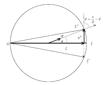
Figure 1. $\theta=<\frac{\xi}{|\xi|}\cdot\sigma>$,  $\vartheta=<\frac{\eta^{+}}{|\eta^{+}|},\sigma>$, $\eta^{+}=\xi^{+}-\zeta$.

We divide the integrand of the left hand side of (3.18) into

$$\int_{\SS^{2}}b\left(\frac{\xi\cdot\sigma}{|\xi|}\right)\Big{(}\varphi(\xi^{+})\varphi(\xi^{-})-\varphi(\xi)\Big{)}d\sigma$$

$$=\int_{\SS^{2}}b\left(\frac{\xi\cdot\sigma}{|\xi|}\right)\Big{(}\varphi(\xi^{+})-\varphi(\xi)\Big{)}d\sigma+\int_{\SS^{2}}b\left(\frac{\xi\cdot\sigma}{|\xi|}\right)\varphi(\xi^{+})\Big{(}\varphi(\xi^{-})-1\Big{)}d\sigma$$

$$=\frac{1}{2}\int_{\SS^{2}}b\left(\frac{\xi\cdot\sigma}{|\xi|}\right)\Big{(}\varphi(\xi^{+})+\varphi(\tilde{\xi}^{+})-2\varphi(\xi)\Big{)}d\sigma$$

$$\qquad\qquad+\int_{\SS^{2}}b\left(\frac{\xi\cdot\sigma}{|\xi|}\right)\varphi(\xi^{+})\Big{(}\varphi(\xi^{-})-1\Big{)}d\sigma$$

$$=\frac{1}{2}\int_{\SS^{2}}b\left(\frac{\xi\cdot\sigma}{|\xi|}\right)\Big{(}\varphi(\xi^{+})+\varphi(\tilde{\xi}^{+})-2\varphi(\zeta)\Big{)}d\sigma$$

$$\quad+\int_{\SS^{2}}b\left(\frac{\xi\cdot\sigma}{|\xi|}\right)\Big{(}\varphi(\zeta)-\varphi(\xi)\Big{)}d\sigma+\int_{\SS^{2}}b\left(\frac{\xi\cdot\sigma}{|\xi|}\right)\varphi(\xi^{+})\Big{(}\varphi(\xi^{-})-1\Big{)}d\sigma$$

$$=I_{1}(\xi)+I_{2}(\xi)+I_{3}(\xi)\,.$$

Putting $\eta^{+}=\xi^{+}-\zeta$, we have

$$|\varphi(\xi^{+})+\varphi(\tilde{\xi}^{+})-2\varphi(\zeta)|=\left|\int_{{{\mathbb{R}}}^{3}}e^{-i\zeta\cdot v}\Big{(}e^{-i\eta^{+}\cdot v}+e^{i\eta^{+}\cdot v}-2\Big{)}dF(v)\right|$$

$$\qquad\leq\int_{{{\mathbb{R}}}^{3}}|e^{-i\zeta\cdot v}|\Big{(}2-e^{-i\eta^{+}\cdot v}-e^{i\eta^{+}\cdot v}\Big{)}dF(v).$$

Noting $|\eta^{+}|=|\xi|\cos(\theta/2)\sin(\theta/2)$ and using the change of variables $\xi\rightarrow(\xi^{+}\rightarrow)\eta^{+}$, we have

$$\int_{{{\mathbb{R}}}^{3}_{\xi}}\frac{|I_{1}(\xi)|}{|\xi|^{3+\alpha}}d\xi \lesssim\int_{{{\mathbb{R}}}^{3}}\frac{|1-\varphi(\pm\eta^{+})|}{|\eta^{+}|^{3+\alpha}}d\eta^{+}\int_{0}^{\pi/2}(\sin\theta)^{1+\alpha}b(\cos\theta)\cos\theta d\theta$$

$$\lesssim\|1-\varphi\|_{{\mathcal{M}}^{\alpha}}\,,$$

where by the same arguments in Section 4 of [6] (cf. [1]), we have used the fact that

$$d\xi=\frac{4d\xi^{+}}{\cos^{2}(\theta/2)}\enskip,\enskip d\xi^{+}=\frac{4d\eta^{+}}{\sin^{2}(\theta/2)}\,\enskip,\enskip d\eta^{+}d\sigma=2\pi\sin\vartheta d\vartheta d\eta^{+}\enskip(\vartheta=\pi/2-\theta)\,.$$

Notice that

(3.19) $$|\varphi(\xi)-\varphi(\xi+\eta)|\leq 4|1-\varphi(\xi)|^{1/2}|1-\varphi(\eta)|^{1/2}+|1-\varphi(\eta)|\,,$$

which was proved in the proof of (19) in [5]. By (3.19) with $\eta=\zeta-\xi$, we have

$$\int_{{{\mathbb{R}}}^{3}_{\xi}}\frac{|I_{2}(\xi)|}{|\xi|^{3+\alpha}}d\xi \lesssim\int_{\SS^{2}}b\left(\frac{\xi\cdot\sigma}{|\xi|}\right)\int_{{{\mathbb{R}}}^{3}}\frac{|1-\varphi(\xi)|^{1/2}|1-\varphi(\zeta-\xi)|^{1/2}}{|\xi|^{3+\alpha}}d\xi d\sigma$$

$$\quad+\int_{\SS^{2}}b\left(\frac{\xi\cdot\sigma}{|\xi|}\right)\int_{{{\mathbb{R}}}^{3}}\frac{|1-\varphi(\zeta-\xi)|}{|\xi|^{3+\alpha}}d\xi d\sigma$$

$$=J_{1}+J_{2}\,.$$

Using the Schwarz inequality, we have

$$J_{1} \leq\int_{\SS^{2}}b\left(\frac{\xi\cdot\sigma}{|\xi|}\right)\Big{(}\int_{{{\mathbb{R}}}^{3}}\frac{|1-\varphi(\xi)|}{|\xi|^{3+\alpha}}d\xi\Big{)}^{1/2}\Big{(}\int_{{{\mathbb{R}}}^{3}}\frac{|1-\varphi(\zeta-\xi)|}{|\xi|^{3+\alpha}}d\xi\Big{)}^{1/2}d\sigma$$

$$=2\pi\|1-\varphi\|_{{\mathcal{M}}^{\alpha}}^{1/2}\Big{(}\int_{{{\mathbb{R}}}^{3}}\frac{|1-\varphi(\eta)|}{|\eta|^{3+\alpha}}d\eta\Big{)}^{1/2}\int_{0}^{\pi/2}b(\cos\theta)\sin^{\alpha}(\theta/2)\sin\theta d\theta$$

$$\lesssim\|1-\varphi\|_{{\mathcal{M}}^{\alpha}}\,,$$

where we have used $|\eta|=|\zeta-\xi|=|\xi|\sin^{2}(\theta/2)$. The estimation for $J_{2}$ is easier, so that we omit its proof. Also since similar estimate holds for $I_{3}(\xi)$, we obtain the desired estimate (3.18). And this completes the proof of the lemma. ∎

3.3. Continuity of measure valued solutions

Finally in this subsection, we discuss the continuity of the solutions obtained above. Assume that $b$ satisfies (1.4) for some $\alpha_{0}\in(0,2)$ and let $\alpha\in[\alpha_{0},2),\alpha\neq 1$. If $F_{0}\in P_{\alpha}({{\mathbb{R}}}^{3})$, then it follows from (1.15) that $\varphi_{0}={\mathcal{F}}(F_{0})$ belongs to ${\mathcal{M}}^{\alpha}$. By Theorem 1.6 and (1.15), there exists a unique measure valued solution $F_{t}\in C([0,\infty),P_{\alpha}({{\mathbb{R}}}^{3}))$ to the Cauchy problem (1.1)-(1.2). Here the continuity with respect to $t$ is in the following sense:

$$\lim_{t\rightarrow t_{0}}\int\psi(v)dF_{t}(v)=\int\psi(v)dF_{t_{0}}(v)\mbox{ for any $\psi\in C({{\mathbb{R}}}^{d})$}$$

      satisfying the growth condition $$|\psi(v)|\lesssim\langle v\rangle^{\alpha}$$.

This continuity follows from the same argument as in the last paragraph of Section 2. Indeed, the fact that ${\mathcal{F}}(F_{t})=\varphi(t,\xi)\in C([0,\infty),{\mathcal{M}}^{\alpha})$ yields

$$\int_{\{|\xi|\leq 1/R\}}\frac{|1-\varphi(t,\xi)|}{|\xi|^{3+\alpha}}d\xi\leq\int_{\{|\xi|\leq 1/R\}}\frac{|1-\varphi(t_{0},\xi)|}{|\xi|^{3+\alpha}}d\xi+\|\varphi(t)-\varphi(t_{0})\|_{{\mathcal{M}}^{\alpha}},$$

and hence for any $\varepsilon>0$, there exist $\delta>0$ and $R>0$ such that

$$\sup_{t\in[t_{0}-\delta,t_{0}+\delta]}\int_{\{|\xi|\leq 1/R\}}\frac{|1-\varphi(t,\xi)|}{|\xi|^{3+\alpha}}d\xi<\varepsilon.$$

This and (2.4) imply that

$$\sup_{t\in[t_{0}-\delta,t_{0}+\delta]}\int_{\{|v|\geq R\}}|v|^{\alpha}dF_{t}(v)<\varepsilon/2c_{\alpha,3,1}.$$

Since $F_{t}\in C([0,\infty),P)$, we have $F_{t}\in C([0,\infty),P_{\alpha})$. Thus Theorem 1.4 is now proved. If $F_{0}\in P_{1}({{\mathbb{R}}}^{3})$ satisfies $\int_{{{\mathbb{R}}}^{3}}\langle v\rangle\log\langle v\rangle dF_{0}(v)<\infty$, then it follows from Proposition 2.1 that $\varphi_{0}={\mathcal{F}}(F_{0})$ belongs to ${\mathcal{M}}^{1}$, and hence the last statement of Remark 1.5 is also obvious. On the other hand, if we simply assume $F_{0}\in P_{1}({{\mathbb{R}}}^{3})$, noting that the index $\alpha_{0}$ of the condition (1.4) is in $(0,1]$, we have a weaker result, (1.17) in Remark 1.5, by means of the following proposition.

Proposition 3.5.

Let $\alpha\geq 1$ and let $b$ satisfy (1.4) with $\alpha_{0}=1$. If the initial data $F_{0}\in P_{\alpha}$, then the unique solution $F_{t}$ belongs to $P_{\alpha}$ for any $t>0$. More precisely, there exists a constant $C>0$ independent of $t$ such that

(3.20) $$\int\langle v\rangle^{\alpha}dF_{t}(v)\leq Ce^{Ct}\int\langle v\rangle^{\alpha}dF_{0}(v)\,.$$

Proof.

For the simplicity of the notations, we consider the case where $F_{0},F_{t}$ have density functions $f_{0}(v),f(t,v)$. For $\delta>0$, put

$$W_{\delta}(v)=\frac{\langle v\rangle^{\alpha}}{1+\delta\langle v\rangle^{\alpha}}\,.$$

Since $x/(1+\delta x)$ is increasing in $[1,\infty]$ and $|v^{\prime}|\leq|v|+|v_{*}|$, we have

$$W_{\delta}(v^{\prime}) \lesssim\frac{\langle v\rangle^{\alpha}+\langle v_{*}\rangle^{\alpha}}{1+\delta(\langle v\rangle^{\alpha}+\langle v_{*}\rangle^{\alpha})}=\frac{\langle v\rangle^{\alpha}}{1+\delta(\langle v\rangle^{\alpha}+\langle v_{*}\rangle^{\alpha})}+\frac{\langle v_{*}\rangle^{\alpha}}{1+\delta(\langle v\rangle^{\alpha}+\langle v_{*}\rangle^{\alpha})}$$

$$\leq\frac{\langle v\rangle^{\alpha}}{1+\delta\langle v\rangle^{\alpha}}+\frac{\langle v_{*}\rangle^{\alpha}}{1+\delta\langle v_{*}\rangle^{\alpha}}=W_{\delta}(v)+W_{\delta}(v_{*})\,.$$

Therefore, $|W_{\delta}(v^{\prime})-W_{\delta}(v)|\lesssim W_{\delta}(v)+W_{\delta}(v_{*})$. If $b_{n}(\cos\theta)=\min\{b(\cos\theta),n\}$ and $f^{n}(t,v)$ is the unique solution of the corresponding Cauchy problem, then we have

$$\frac{d}{dt}\int f^{n}(t,v)W_{\delta}(v)dv\lesssim\Big{(}\int b_{n}d\sigma\Big{)}\Big{(}\int f^{n}(t,v)W_{\delta}(v)dv\Big{)}\Big{(}\int f^{n}(t,v_{*})dv_{*}\Big{)}\,,$$

which yields

$$\int f^{n}(t,v)W_{\delta}(v)dv\leq C_{n}e^{C_{n}t}\int f_{0}(v)W_{\delta}(v)dv.$$

Taking the limit $\delta\rightarrow+0$, we have $f^{n}(t,v)\in L^{1}_{\alpha}$. Note that

$$\langle v^{\prime}\rangle^{\alpha}-\langle v\rangle^{\alpha}\lesssim\big{(}\langle v\rangle^{\alpha-1}+\langle v_{*}\rangle^{\alpha-1}\big{)}|v-v_{*}|\sin\frac{\theta}{2},$$

because $\alpha\geq 1$. Then, there exists a constant $C>0$ independent of $n$ such that

$$\frac{d}{dt}\int f^{n}(t,v)\langle v\rangle^{\alpha}dv \leq\Big{(}\int b_{n}\theta d\sigma\Big{)}\Big{(}\int f^{n}(t,v)\langle v\rangle^{\alpha}dv\Big{)}\Big{(}\int f^{n}(t,v_{*})dv_{*}\Big{)}$$

$$\leq C\int f^{n}(t,v)\langle v\rangle^{\alpha}dv\,.$$

We have $\int f^{n}(t,v)\langle v\rangle^{\alpha}dv\leq Ce^{Ct}\int f_{0}(v)\langle v\rangle^{\alpha}dv$. Take a cutoff function $\chi(v)$ in $C_{0}^{\infty}({{\mathbb{R}}}^{3})$ satisfying $0\leq\chi\leq 1$ and $\chi=1$ on $\{|v|\leq 1\}$. Then, for any $m\in{\mathbb{N}}$, we have

$$\int f^{n}(t,v)\langle v\rangle^{\alpha}\chi\left(\frac{v}{m}\right)dv\leq Ce^{Ct}\int f_{0}(v)\langle v\rangle^{\alpha}dv.$$

Since $f^{n}(t,v)\rightarrow f(t,v)$ in ${\mathcal{S}}^{\prime}({{\mathbb{R}}}^{3}_{v})$ and $\langle v\rangle^{\alpha}\chi\left(\frac{v}{m}\right)\in{\mathcal{S}}$, we get

$$\int f(t,v)\langle v\rangle^{\alpha}\chi\left(\frac{v}{m}\right)dv\leq Ce^{Ct}\int f_{0}(v)\langle v\rangle^{\alpha}dv.$$

Letting $m\rightarrow\infty$ gives the desired estimate (3.20). And this completes the proof of the proposition. ∎

4. Proof of Theorem 1.8

In this section, we will show that the measure valued solutions obtained in both the function spaces ${\mathcal{K}}^{\alpha}$ and ${\mathcal{M}}^{\alpha}$ is $H^{\infty}_{v}$ for any positive time, under the angular singularity assumption (1.3) on the cross section.

For this, we first recall that in the proof of Theorem 1.3 of [7], we already showed that, if $F_{0}\in\tilde{P}_{\alpha}({{\mathbb{R}}}^{3})$, then there exists a $T>0$ such that the unique solution $f(t,v)\in C([0,\infty),\tilde{P}_{\alpha})$ ($\alpha>2s$) satisfies

$$f(t,v)\in H^{\infty}({{\mathbb{R}}}^{3})\enskip\mbox{for any fixed}\enskip t\in(0,T]\,.$$

This local smoothing effect was extended to the global one in the case when the initial datum belongs to $P_{2}$, by using the energy conservation law and the uniform boundedness of the entropy norm (see (1.12) of [7]).

In order to prove the global in time smoothing effect even for infinite energy solutions, instead of (1.12) in [7], we will show that for any $T_{1}>T$, there exists a $C_{T_{1}}>0$ such that

(4.1) $$\sup_{T\leq t\leq T_{1}}\Big{(}\|f(t)\|_{L^{1}_{\alpha^{\prime}}}+\|f(t)\|_{L\log L}\Big{)}<C_{T_{1}},$$

for any $\alpha^{\prime}<\alpha$. Based on (4.1), we will then show the global in time smoothing effect, that is, $f(t,v)\in H^{\infty}({{\mathbb{R}}}^{3})$ for any $t>T$.

The bound of the first term in (4.1) is now clear. In fact, by using (2.5) and (2.6), we have

(4.2) $$\||v|^{\alpha^{\prime}}f(t)\|_{L^{1}}\leq\frac{C_{\alpha^{\prime},\alpha,3}}{2c_{\alpha^{\prime},3,\infty}}\big{(}\|\varphi(t)-1\|_{\alpha}\big{)}^{\alpha^{\prime}/\alpha}\leq\frac{C_{\alpha^{\prime},\alpha,3}}{2c_{\alpha^{\prime},3,\infty}}\big{(}e^{\lambda_{\alpha}t}\|\varphi_{0}-1\|_{\alpha}\big{)}^{\alpha^{\prime}/\alpha}\,,$$

where we have used (1.22) to get the second inequality. It remains to show the boundedness of the second term in (4.1).

It follows from the local smoothing effect that $\int f(T,v)\log(1+f(T,v))dv<\infty$. Writing $0$ and $\alpha$ instead of $T$ and $\alpha^{\prime}$, respectively, for simplicity, we show the following;

Proposition 4.1.

Let $b(\cos\theta)$ satisfy (1.3) with $0<s<1$. Let $2s<\alpha<2$. Assume that $0\leq f_{0}\in L^{1}_{\alpha}({{\mathbb{R}}}^{3})\cap L\log L({{\mathbb{R}}}^{3})$ and $\int f_{0}(v)dv=1$. If $f(t,v)$ is the unique solution in $C([0,\infty),\tilde{P}_{\alpha})$ of the Cauchy problem (1.1)-(1.2), then $f(t,v)\in L^{\infty}_{loc}([0,\infty),L^{1}_{\alpha}({{\mathbb{R}}}^{3})\cap L\log L({{\mathbb{R}}}^{3}))$, that is, for any $T_{1}>0$ there exists a $C_{T_{1}}>0$ such that

(4.3) $$\sup_{0<t\leq T_{1}}\int\langle v\rangle^{\alpha}f(t,v)dv+\int f(t,v)\log\big{(}1+f(t,v)\big{)}dv\leq C_{T_{1}}\,.$$

Proof.

Since we assume $f_{0}\in L^{1}_{\alpha}({{\mathbb{R}}}^{3})$, there exists $C>0$ such that

(4.4) $$\int\langle v\rangle^{\alpha}f(t,v)dv\leq Ce^{Ct}\int\langle v\rangle^{\alpha}f_{0}(v)dv.$$

In fact, when $\alpha\neq 1$, it follows from (2.5), (1.21) and (2.1) that

(4.5) $$\||v|^{\alpha}f(t)\|_{L^{1}}\leq\frac{1}{2c_{\alpha,3,\infty}}\|\varphi(t)-1\|_{{\mathcal{M}}^{\alpha}}\leq\frac{e^{\lambda_{\alpha}t}}{2c_{\alpha,3,\infty}}\|\varphi_{0}-1\|_{{\mathcal{M}}^{\alpha}}\lesssim e^{\lambda_{\alpha}t}\|f_{0}\|_{L^{1}_{\alpha}}\,.$$

The exceptional case $\alpha=1$ follows from Proposition 3.5, because of $2s<\alpha=1$. We will show the boundedness of the second term in (4.3). Take the same cutoff function $\chi(v)$ in $C_{0}^{\infty}({{\mathbb{R}}}^{3})$ as in the proof of Proposition 3.5. For $m\in{\mathbb{N}}$, put $\tilde{f}_{0,m}(v)=c_{m}\chi\left(\frac{v}{m}\right)f_{0}(v)$ with $c_{m}=1/\int\chi\left(\frac{v}{m}\right)f_{0}(v)dv$. Since $f_{0}(v)\in L^{1}_{\alpha}({{\mathbb{R}}}^{3})$, there exists $M\in{\mathbb{N}}$ such that $1\leq c_{m}\leq 2$ for all $m\geq M$.

We consider only the case $s\geq 1/2$ because the case when $0<s<1/2$ is easier. For $a_{m}=\int v\tilde{f}_{0,m}(v)dv$, put $f_{0,m}(v)=\tilde{f}_{0,m}(v+a_{m})$. Since $|a_{m}|^{\alpha}\leq 2\int\langle v\rangle^{\alpha}f_{0}dv$, it follows from Lemma 3.15 of [2] that $\{f_{0,m}\}$ belongs to a bounded set of $\tilde{P}_{\alpha}$, equivalently, $\{\hat{f}_{0,m}\}$ belongs to a bounded set of ${\mathcal{K}}^{\alpha}$, that is,

(4.6) $$\|1-\hat{f}_{0,m}\|_{\alpha}\lesssim\int\langle v\rangle^{\alpha}f_{0}(v)dv\,.$$

Consider the solutions $f_{m}(t,v)$ for the Cauchy problem with the initial data $f_{0,m}(v)$ with $m\geq M$. Since $f_{0,m}\in L^{1}_{2}({{\mathbb{R}}}^{3})\cap L\log L({{\mathbb{R}}}^{3})$, we have by Theorem 1 of [9] that

(4.7) $$\int f_{m}(t,v)\log f_{m}(t,v)dv+\int_{0}^{t}D(f_{m})(s)ds=\int f_{0,m}(v)\log f_{0,m}(v)dv\,,$$

where $D(f)(t)$ is defined by

$$D(f)(t)=\frac{1}{4}\iiint_{{{\mathbb{R}}}^{3}\times{{\mathbb{R}}}^{3}\times\SS^{2}}b(f^{\prime}_{*}f^{\prime}-f_{*}f)\log\frac{f^{\prime}_{*}f^{\prime}}{f_{*}f}dvdv_{*}d\sigma\geq 0,$$

with $f=f(t,\cdot)$. Therefore, writing $\chi_{m}=\chi(v/m)$, we have

$$\int f_{m}(t,v)\log f_{m}(t,v)dv\leq\int f_{0,m}(v)\log f_{0,m}(v)dv$$

$$\leq 2\log 2\int f_{0}dv+2\int\chi_{m}f_{0}\log^{+}\chi_{m}f_{0}dv.$$

Noting that $x\log x\geq-y+x\log y$ $(x\geq 0,y>0)$, we have

$$0\geq f_{m}(t,v)\log^{-}f_{m}(t,v)\geq-e^{-\langle v\rangle^{\alpha}}-\langle v\rangle^{\alpha}f_{m}(t,v),$$

which together with (4.4) yields,

$$\int f_{m}(t,v)\log^{+}f_{m}(t,v)dv\leq 2\log 2\int f_{0}dv$$

$$\quad+2\int f_{0}(v)\log^{+}f_{0}(v)dv+\int e^{-\langle v\rangle^{\alpha}}dv+4Ce^{Ct}\int\langle v\rangle^{\alpha}f_{0}(v)dv,$$

because $\int\langle v\rangle^{\alpha}f_{0,m}dv\leq 4\int\langle v\rangle^{\alpha}f_{0}dv$. Thus, for any $T>0$ there exists $C^{\prime}_{T}>0$ such that

$$\sup_{0<t\leq T}\Big{(}\int\langle v\rangle^{\alpha}f_{m}(t,v)dv+\int f_{m}(t,v)\log(1+f_{m}(t,v))dv\Big{)}\leq C^{\prime}_{T}\,,$$

which concludes the weak compactness of $\{f_{m}\}$ in $L^{1}({{\mathbb{R}}}^{3})$, by means of Dunford-Pettis criterion. Notice (4.6) again, namely the fact that $\hat{f}_{0,m},\hat{f}_{0}\in{\mathcal{K}}^{\alpha}$ uniformly with respect to $m$. Take a $\alpha^{\prime}\in(2s,\alpha)$. For any $\delta>0$ we have

$$\sup_{0<|\xi|<\delta}\frac{|\hat{f}_{0,m}(\xi)-\hat{f}_{0}(\xi)|}{|\xi|^{\alpha^{\prime}}} \leq\delta^{\alpha-\alpha^{\prime}}\Big{(}\sup_{0<|\xi|<\delta}\frac{|\hat{f}_{0,m}(\xi)-1|}{|\xi|^{\alpha}}+\sup_{0<|\xi|<\delta}\frac{|1-\hat{f}_{0}(\xi)|}{|\xi|^{\alpha}}\Big{)}$$

$$\lesssim\delta^{\alpha-\alpha^{\prime}}\int\langle v\rangle^{\alpha}f_{0}(v)dv\,.$$

Note that for any $R>0$ large enough, we have

$$\sup_{|\xi|>R}\frac{|\hat{f}_{0,m}(\xi)-\hat{f}_{0}(\xi)|}{|\xi|^{\alpha^{\prime}}}\leq 2R^{-\alpha^{\prime}}\,.$$

In view of (4.6), it follows from Lemma 2.1 of [5] that $\{\hat{f}_{0,m}\}$ is uniformly equi-continuous on the compact set $\{\delta\leq|\xi|\leq R\}$. By the Ascoli-Arzelá theorem, $\{\hat{f}_{0,m}\}$ is a Cauchy sequence in $\|\cdot\|_{\alpha^{\prime}}$, taking a subsequence if necessary. Since $f_{0,m}(v)\rightarrow f_{0}(v)$ in ${\mathcal{S}}^{\prime}({{\mathbb{R}}}^{3})$ as $m$ tends to $\infty$, we concludes $\|\hat{f}_{0,m}-\hat{f}_{0}\|_{\alpha^{\prime}}\rightarrow 0$.

It follows from (1.22) that

$$\|\hat{f}_{m}(t,\cdot)-\hat{f}(t,\cdot)\|_{\alpha^{\prime}}\leq e^{\lambda_{\alpha^{\prime}}t}\|\hat{f}_{0,m}-\hat{f}_{0}\|_{\alpha^{\prime}},$$

which implies that $\hat{f}_{m}(t,\xi)\rightarrow\hat{f}(t,\xi)$ everywhere in $\xi$ for any fixed $t>0$. Since

$$|\hat{f}_{m}(t,\xi)|,\quad|\hat{f}(t,\xi)|\leq 1,$$

we know $f_{m}(t,v)\rightarrow f(t,v)$ in ${\mathcal{S}}^{\prime}({{\mathbb{R}}}^{3})$. If we recall the weak compactness of $\{f_{m}(t,\cdot)\}$ in $L^{1}({{\mathbb{R}}}^{3})$, then we obtain

$$f_{m}(t,\cdot)\rightarrow f(t,\cdot)\enskip\mbox{weekly in }\enskip L^{1}({{\mathbb{R}}}^{3}).$$

Since $\lambda\log(1+\lambda)$ is convex, for $0<t\leq T$, we have

$$\int f(t,v)\log(1+f(t,v))dv\leq\lim\inf\int f_{m}(t,v)\log(1+f_{m}(t,v))dv\leq C^{\prime}_{T}.$$

And this completes the proof of the proposition. ∎

Since the global in time smoothing effect has been established, that is, $f(t,v)\in H^{\infty}({{\mathbb{R}}}^{3})$ for any $t>0$, it follows from Theorem 1.4 together with Remark 1.5 that $f(t,v)\in L^{1}_{\alpha}({{\mathbb{R}}}^{3})$ for $t>0$ if $F_{0}\in P_{\alpha}({{\mathbb{R}}}^{3})$. To complete the proof of Theorem 1.8 , it remains to show $f(t)\in$ $C((0,\infty),L^{1}_{\alpha}({{\mathbb{R}}}^{3})\cap H^{\infty}({{\mathbb{R}}}^{3}))$ if $F_{0}\in P_{\alpha}({{\mathbb{R}}}^{3})$ and $\alpha\neq 1$. Let $0<T_{1}<T_{2}$, Since it follows from (3.17) that

$$\|\varphi(t)-\varphi(t_{0})\|_{{\mathcal{M}}^{\alpha}}\lesssim|t-t_{0}|\,,\enskip t,t_{0}\in[T_{1},T_{2}],$$

by the same argument as the one given in the last paragraph of Section 2, we see that for any $\varepsilon>0$ there exist $R>1$ and $\delta>0$ such that

(4.8) $$\int_{\{|v|\geq R\}}|v|^{\alpha}f(t,v)dv<\varepsilon\,\enskip\mbox{if $|t-t_{0}|<\delta$}.$$

Then for any $M>1$, we have

$$|f(t,v)-f(t_{0},v)| \leq\int|\varphi(t,\xi)-\varphi(t_{0},\xi)|d\xi$$

$$\leq 2\sup_{\tau\in[T_{1},T_{2}]}\|f(\tau)\|_{H^{2}({{\mathbb{R}}}^{3})}\Big{(}\int_{\{|\xi|\geq M\}}\langle\xi\rangle^{-4}d\xi\Big{)}^{1/2}$$

$$\quad+\|\varphi(t)-\varphi(t_{0})\|_{\alpha}\int_{\{|\xi|<M\}}|\xi|^{\alpha}d\xi\,,$$

which together with (4.8) imply that $f(t)\in C((0,\infty),L^{1}_{\alpha}({{\mathbb{R}}}^{3}))$. In view of (4.1), it follows from the proof of Theorem 1.5 in [5] that for any $N\in{\mathbb{N}}$ there exists a $C_{N}>0$ such that

$$\sup_{T_{1}\leq\tau\leq T_{2}}\int|\langle\xi\rangle^{N+1}\varphi(\tau,\xi)|^{2}d\xi\leq C_{N}.$$

Noticing that for any $R>1$

$$\|f(t)-f(t_{0})\|^{2}_{H^{N}}\leq(1+R^{2})^{N}\int_{\{|\xi|\leq R\}}|\varphi(t,\xi)-\varphi(t_{0},\xi)|^{2}d\xi+4C_{N}R^{-2},$$

we have $f(t)\in C((0,\infty),H^{N}({{\mathbb{R}}}^{3}))$ because of $\varphi(t)\in C([0,\infty),{\mathcal{K}}^{\alpha})$.

Acknowledgements: The research of the first author was supported in part by Grant-in-Aid for Scientific Research No.25400160, Japan Society of the Promotion of Science. The research of the third author was supported in part by the General Research Fund of Hong Kong, CityU No.104511, and the Shanghai Jiao Tong University.

References

- [1] R. Alexandre, L. Desvillettes, C. Villani and B. Wennberg, Entropy dissipation and long-range interactions, Arch. Rational Mech. Anal. 152 (2000), 327-355.
- [2] M. Cannone and G. Karch, Infinite energy solutions to the homogeneous Boltzmann equation, Comm. Pure Appl. Math. 63 (2010), 747-778.
- [3] E. A. Carlen, E. Gabetta and G. Toscani, Propagation of smoothness and the rate of exponential convergence to equilibrium for a spatially homogeneous Maxwellian gas, Comm. Math. Phys., 199 (1999) 521-546.
- [4] E. Gabetta, G. Toscani and B. Wennberg, Metrics for probability distributions and the rend to equilibrium for solutions of the Boltzmann equation, J. Statist. Phys, 81, 901-934.
- [5] Y. Morimoto, A remark on Cannone-Karch solutions to the homogeneous Boltzmann equation for Maxwellian molecules, Kinetic and Related Models, 5 (2012), 551-561.
- [6] Y. Morimoto, S. Ukai, C.-J. Xu and T. Yang, Regularity of solutions to the spatially homogeneous Boltzmann equation without angular cutoff, Discrete and Continuous Dynamical Systems - Series A 24 (2009), 187–212.
- [7] Y. Morimoto and T. Yang, Smoothing effect of the homogeneous Boltzmann equation with measure valued initial datum, to appear in Ann. Inst. H. Poincaré Anal. Non Linéaire.
- [8] G. Toscani and C. Villani, Probability metrics and uniqueness of the solution to the Boltzmann equations for Maxwell gas, J. Statist. Phys., 94 (1999), 619-637.
- [9] C. Villani, On a new class of weak solutions to the spatially homogeneous Boltzmann and Landau equations, Arch. Rational Mech. Anal., 143 (1998), 273–307.
- [10] C. Villani, A review of mathematical topics in collisional kinetic theory. In: Friedlander S., Serre D. (ed.), Handbook of Fluid Mathematical Fluid Dynamics, Elsevier Science (2002).
- [11] C. Villani, Topics in optimal transportation. Graduate Studies in Mathematics, 58. American Mathematical Society, Providence, RI, (2003) .