Violation of PCAC and two-body baryonic $B$ and $D_{s}$ decays

Abstract

We study the two-body baryonic $B$ and $D_{s}$ decays based on the annihilation mechanism without the partial conservation of axial-vector current (PCAC) at the GeV scale. We demonstrate that the contributions of $B^{-}\to\Lambda\bar{p}$, $B^{-}\to\Sigma^{0}\bar{p}$ and $\bar{B}^{0}_{s}\to\Lambda\bar{\Lambda}$ are mainly from the scalar and pseudoscalar currents with their branching ratios predicted to be around $(3.5,\,5.3,\,5.3)\times 10^{-8}$, respectively, exactly the sizes of ${\cal B}(B\to{\bf B\bar{B}^{\prime}})$ established by the data. We also apply the annihilation mechanism to all of the charmless two-body baryonic $B$ and $D_{s}$ decays. In particular, we can explain ${\cal B}(\bar{B}^{0}_{(s)}\to p\bar{p})$ of order $10^{-8}$ and ${\cal B}(D_{s}^{+}\to p\bar{n})$ of order $10^{-3}$, which are from the axial-vector currents. In addition, the branching ratios of $\bar{B}^{0}\to\Lambda\bar{\Lambda}$, $B^{-}\to n\bar{p}$, and $B^{-}\to\Sigma^{-}\bar{\Sigma}^{0}$ are predicted to be $(0.3,\,3.2,\,9.6)\times 10^{-8}$, which can be measured by LHCb and viewed as tests for the violation of PCAC at the GeV scale.

I Introduction

For the abundantly observed three-body baryonic $B$ decays ($B\to{\bf B\bar{B}^{\prime}}M$), the theoretical approach for the systematic study has been established HouSoni ; Cheng:2001tr ; ChuaHou ; ChuaHouTsai ; AngdisppK ; NF_GengHsiao . It leads to the theoretical predictions, among which at least five decay modes GengHsiao5 ; GengHsiaoHY are observed to agree with the data pdg . On the other hand, the two-body baryonic $B$ decays ($B\to{\bf B\bar{B}^{\prime}}$) are poorly understood due to the smaller branching ratios, causing a much later observation than $B\to{\bf B\bar{B}^{\prime}}M$. Recently, the LHCb collaboration has presented the first observations of the charmless $B\to{\bf B\bar{B}^{\prime}}$ decays Aaij:2013fta , given by

$${\cal B}(\bar{B}^{0}\to p\bar{p}) = (1.47^{+0.62+0.35}_{-0.51-0.14})\times 10^{-8}\,,$$

$${\cal B}(\bar{B}^{0}_{s}\to p\bar{p}) = (2.84^{+2.03+0.85}_{-1.68-0.18})\times 10^{-8}\,,$$ (1)

with the statistical significances to be $3.3\sigma$ and $1.9\sigma$, respectively.

Based on the factorization, when the $B$ meson annihilates with the momentum transfer $q$, the amplitudes ${\cal A}(\bar{B}^{0}_{(s)}\to p\bar{p})$ can be decomposed as $q^{\mu}\langle p\bar{p}|A_{\mu}|0\rangle$, where the matrix element is for the proton pair production and $A_{\mu}$ is the axial-vector current. From the hypothesis of the partial conservation of the axial-vector current (PCAC) PCAC at the GeV scale, $q^{\mu}A_{\mu}$ is proportional to $m_{\pi}^{2}$, which leads to ${\cal A}(\bar{B}^{0}_{(s)}\to p\bar{p})\simeq 0$. This is the reason why the non-factorizable effects were believed to dominate the branching ratios in Eq. (I) diagramic1 . However, since the predictions from these models differ from each other, and commonly exceed the data, a reliable theoretical approach has not been established yet.

In this work, we would propose a new method without the use of PCAC. In fact, the smallness of the previous estimations is not caused by the annihilation mechanism Pham:1980dc , but the assumption of PCAC. Moreover, this assumption has never been tested at the GeV scale. For example, ${\cal B}(B^{-}\to\Lambda\bar{p})$ and ${\cal B}(\bar{B}^{0}_{s}\to\Lambda\bar{\Lambda})$ are found to have the amplitudes decomposed as $({m_{B}^{2}}/{m_{b}})\langle p\bar{p}|S+P|0\rangle$ with $S(P)$ the (pseudo)scalar current, which has no connection to PCAC. Since they can be estimated to be of order $10^{-8}$, exactly the order of the magnitude of ${\cal B}(B\to{\bf B\bar{B}^{\prime}})$ measured by the experiments, the annihilation mechanism can be justified. If the axial-vector current is asymptotically conserved, the result of ${\cal B}(D_{s}^{+}\to p\bar{n})=(0.4^{+1.1}_{-0.3})\times 10^{-6}$ in Ref. Chen:2008pf would yield ${\cal B}(D_{s}^{+}\to p\bar{n})/{\cal B}(D_{s}^{+}\to\tau\bar{\nu}_{\tau})\simeq 10^{-5}$, which was indeed suggested as the test of PCAC at the GeV scale Pham:1980dc . Nonetheless, with ${\cal B}(D_{s}^{+}\to p\bar{n})$$=(1.30\pm 0.36^{+0.12}_{-0.16})\times 10^{-3}$ measured by the CLEO Collaboration Athar:2008ug , one obtains that ${\cal B}(D_{s}^{+}\to p\bar{n})/{\cal B}(D_{s}^{+}\to\tau\bar{\nu}_{\tau})\simeq 0.02$, which is too large and can be viewed as a counter case of PCAC Bediaga:1991eu .

In this paper, we apply the annihilation mechanism to the two-body baryonic $B$ decays, provided that the axial-vector current is not asymptotically conserved. By modifying the timelike baryonic form factors via the axial-vector current without respect to PCAC, we can explain ${\cal B}(\bar{B}^{0}_{(s)}\to p\bar{p})$ as well as ${\cal B}(D_{s}^{+}\to p\bar{n})$. We shall also predict ${\cal B}(B^{-}\to\Lambda(\Sigma^{0})\bar{p})$ and ${\cal B}(\bar{B}^{0}_{s}\to\Lambda\bar{\Lambda})$ in terms of the timelike baryonic form factors via the scalar and pseudoscalar currents.

The paper is organized as follows. In Sec. 2, we present the formalism of the two-body baryonic $B$ and $D_{s}$ decays. In Sec. 3, we proceed our numerical analysis. Sec. 4 contains our discussions and conclusions.

II Formalism

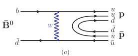
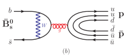
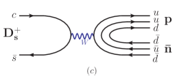
Figure 1: The two-body baryonic decays of (a)$\bar{B}^{0}\to p\bar{p}$, (b)$\bar{B}^{0}_{s}\to p\bar{p}$, and (c)$D^{+}_{s}\to p\bar{n}$.

The non-leptonic $B$ and $D$ decays in the factorization hypothesis are in analogy with the semileptonic cases like ${\cal A}(B\to\pi e\bar{\nu}_{e})\propto\langle\pi|u\gamma^{\mu}(1-\gamma_{5})b|B\rangle\bar{e}\gamma_{\mu}(1-\gamma_{5})\nu_{e}$ to have the amplitudes with an additional matrix element in the form of $\langle X_{2}|J^{2(\mu)}|0\rangle\langle X_{1}|J^{1}_{(\mu)}|B\rangle$, where $J^{1,2}_{(\mu)}$ are the quark currents, and $X_{1,2}$ can be multi-hadron states fac1 ; fac2 . Although the derivation may not be analytically satisfactory, the factorization approximation can still be justified by theoretically reproducing the data and predicting not-yet-observed decay modes to be approved by the later measurements in the two-body and three-body mesonic $B$ decays as well as the three-body baryonic $B$ decays GengHsiaoHY ; ali ; Hamiltonian ; 3b_HY .

Like the measured $\bar{B}^{0}_{(s)}\to p\bar{p}$ and $D_{s}^{+}\to p\bar{n}$ with the decaying processes depicted in Fig. 1, in the two-body baryonic $B$ and $D_{s}$ decays, the factorizable amplitudes are known to depend on the annihilation mechanism Pham:1980dc ; Bediaga:1991eu , where $B$ and $D_{s}$ annihilate, followed by the baryon pair production. Thus, the amplitudes can have two types, ${\cal A}_{1}$ and ${\cal A}_{2}$, which consist of (axial)vectors and (pseudo)scalar quark currents, respectively. For example, the amplitudes of $\bar{B}^{0}\to(p\bar{p}$, $\Lambda\bar{\Lambda})$, $B^{-}\to(n\bar{p}$, $\Sigma^{-}\bar{\Sigma}^{0})$, and $D_{s}^{+}\to p\bar{n}$ are of the first type, given by Pham:1980dc ; Bediaga:1991eu ; Chen:2008pf

$${\cal A}_{1}(\bar{B}^{0}\to{\bf B_{1}\bar{B}_{1}^{\prime}})=\frac{G_{F}}{\sqrt{2}}V_{ub}V_{ud}^{*}\,a_{2}\langle{\bf B_{1}\bar{B}_{1}^{\prime}}|(\bar{u}u)_{V-A}|0\rangle\langle 0|(\bar{d}b)_{V-A}|\bar{B}^{0}\rangle\,,$$

$${\cal A}_{1}(B^{-}\to{\bf B_{2}\bar{B}_{2}^{\prime}})=\frac{G_{F}}{\sqrt{2}}V_{ub}V_{ud}^{*}\,a_{1}\langle{\bf B_{2}\bar{B}_{2}^{\prime}}|(\bar{d}u)_{V-A}|0\rangle\langle 0|(\bar{u}b)_{V-A}|B^{-}\rangle\,,$$

$${\cal A}_{1}(D_{s}^{+}\to p\bar{n})=\frac{G_{F}}{\sqrt{2}}V_{cs}V_{ud}^{*}\,a_{1}\langle p\bar{n}|(\bar{u}d)_{V-A}|0\rangle\langle 0|(\bar{s}c)_{V-A}|D^{+}_{s}\rangle\,,$$ (2)

where ${\bf B_{1}\bar{B}_{1}^{\prime}}=p\bar{p}$ or $\Lambda\bar{\Lambda}$, ${\bf B_{2}\bar{B}_{2}^{\prime}}=n\bar{p}$ or $\Sigma^{-}\bar{\Sigma}^{0}$, $(\bar{q}_{1}q_{2})_{V-A}$ denotes $\bar{q}_{1}\gamma_{\mu}(1-\gamma_{5})q_{2}$, $G_{F}$ is the Fermi constant, $a_{i}$ are the effective Wilson coefficients, and $V_{q_{1}q_{2}}$ are the Cabibbo-Kobayashi-Maskawa (CKM) matrix elements. The amplitudes of $\bar{B}^{0}_{s}\to(p\bar{p}$, $\Lambda\bar{\Lambda})$ and $B^{-}\to(\Lambda\bar{p}$, $\Sigma^{0}\bar{p})$ are more complicated, written as

$${\cal A}(\bar{B}^{0}_{s}\to{\bf B_{1}\bar{B}_{1}^{\prime}})={\cal A}_{1}(\bar{B}^{0}_{s}\to{\bf B_{1}\bar{B}_{1}^{\prime}})+{\cal A}_{2}(\bar{B}^{0}_{s}\to{\bf B_{1}\bar{B}_{1}^{\prime}})\,,$$

$${\cal A}(B^{-}\to{\bf B_{2}\bar{B}_{2}^{\prime}})={\cal A}_{1}(B^{-}\to{\bf B_{2}\bar{B}_{2}^{\prime}})+{\cal A}_{2}(B^{-}\to{\bf B_{2}\bar{B}_{2}^{\prime}})\,,$$ (3)

where

$${\cal A}_{1}(\bar{B}^{0}_{s}\to{\bf B_{1}\bar{B}_{1}^{\prime}}) = \frac{G_{F}}{\sqrt{2}}\bigg{\{}V_{ub}V_{us}^{*}\,a_{2}\langle{\bf B_{1}\bar{B}_{1}^{\prime}}|(\bar{u}u)_{V-A}|0\rangle$$

$$-V_{tb}V_{ts}^{*}\bigg{[}a_{3}\langle{\bf B_{1}\bar{B}_{1}^{\prime}}|(\bar{u}u+\bar{d}d+\bar{s}s)_{V-A}|0\rangle$$

$$+a_{4}\langle{\bf B_{1}\bar{B}_{1}^{\prime}}|(\bar{s}s)_{V-A}|0\rangle+a_{5}\langle{\bf B_{1}\bar{B}_{1}^{\prime}}|(\bar{u}u+\bar{d}d+\bar{s}s)_{V+A}|0\rangle$$

$$+\frac{a_{9}}{2}\langle{\bf B_{1}\bar{B}_{1}^{\prime}}|(2\bar{u}u-\bar{d}d-\bar{s}s)_{V-A}|0\rangle\bigg{]}\bigg{\}}\langle 0|(\bar{s}b)_{V-A}|\bar{B}^{0}_{s}\rangle\,,$$

$${\cal A}_{1}(B^{-}\to{\bf B_{2}\bar{B}_{2}^{\prime}}) = \frac{G_{F}}{\sqrt{2}}(V_{ub}V_{us}^{*}\,a_{1}-V_{tb}V_{ts}^{*}\,a_{4})\langle{\bf B_{2}\bar{B}_{2}^{\prime}}|(\bar{s}u)_{V-A}|0\rangle\langle 0|(\bar{u}b)_{V-A}|B^{-}\rangle\,,~{}~{}$$ (4)

and

$${\cal A}_{2}(\bar{B}^{0}_{s}\to{\bf B_{1}\bar{B}_{1}^{\prime}}) = \frac{G_{F}}{\sqrt{2}}V_{tb}V_{ts}^{*}\,2a_{6}\langle{\bf B_{1}\bar{B}_{1}^{\prime}}|(\bar{s}s)_{S+P}|0\rangle\langle 0|(\bar{s}b)_{S-P}|\bar{B}^{0}_{s}\rangle\,,$$

$${\cal A}_{2}(B^{-}\to{\bf B_{2}\bar{B}_{2}^{\prime}}) = \frac{G_{F}}{\sqrt{2}}V_{tb}V_{ts}^{*}\,2a_{6}\langle{\bf B_{2}\bar{B}_{2}^{\prime}}|(\bar{s}u)_{S+P}|0\rangle\langle 0|(\bar{u}b)_{S-P}|B^{-}\rangle\,,$$ (5)

with ${\bf B_{1}\bar{B}_{1}^{\prime}}=p\bar{p}$ or $\Lambda\bar{\Lambda}$, ${\bf B_{2}\bar{B}_{2}^{\prime}}=\Lambda\bar{p}$ or $\Sigma^{0}\bar{p}$, and $(\bar{q}_{1}q_{2})_{S\pm P}$ representing $\bar{q}_{1}(1\pm\gamma_{5})q_{2}$. For the coefficients $a_{i}$ in Eqs. (II)-(II), we use the same inputs as those in $B\to{\bf B\bar{B}^{\prime}}M$ GengHsiao5 ; GengHsiaoHY , where $a_{i}=c^{eff}_{i}+c^{eff}_{i\pm 1}/N_{c}$ with the color number $N_{c}$ for $i=$odd (even) in terms of the effective Wilson coefficients $c^{eff}_{i}$, defined in Refs. Hamiltonian ; ali . Note that $N_{c}$ is floating between 2 and $\infty$ in the generalized factorization for the correction of the non-factorizable effects. In Eqs. (II)-(II), the matrix element for the annihilation of the pseudoscalar meson is defined by

$$\langle 0|\bar{q}_{1}\gamma_{\mu}\gamma_{5}q_{2}|P\rangle = if_{P}q_{\mu}\,,$$ (6)

with $f_{P}$ the decay constant, from which we can obtain $\langle 0|\bar{q}_{1}\gamma_{5}q_{2}|P\rangle$ by using the the equation of motion: $-i\partial^{\mu}(\bar{q}_{1}\gamma_{\mu}q_{2})=(m_{q_{1}}-m_{q_{2}})\bar{q}_{1}q_{2}$ and $-i\partial^{\mu}(\bar{q}_{1}\gamma_{\mu}\gamma_{5}q_{2})=(m_{q_{1}}+m_{q_{2}})\bar{q}_{1}\gamma_{5}q_{2}$. For the dibaryon production, the matrix elements read

$$\langle{\bf B}{\bf\bar{B}^{\prime}}|\bar{q}_{1}\gamma_{\mu}q_{2}|0\rangle = \bar{u}\bigg{\{}F_{1}\gamma_{\mu}+\frac{F_{2}}{m_{\bf B}+m_{\bf\bar{B}^{\prime}}}i\sigma_{\mu\nu}q_{\mu}\bigg{\}}v\;,$$

$$\langle{\bf B}{\bf\bar{B}^{\prime}}|\bar{q}_{1}\gamma_{\mu}\gamma_{5}q_{2}|0\rangle = \bar{u}\bigg{\{}g_{A}\gamma_{\mu}+\frac{h_{A}}{m_{\bf B}+m_{\bf\bar{B}^{\prime}}}q_{\mu}\bigg{\}}\gamma_{5}v\,,$$

$$\langle{\bf B}{\bf\bar{B}^{\prime}}|\bar{q}_{1}q_{2}|0\rangle = f_{S}\bar{u}v\;,$$

$$\langle{\bf B}{\bf\bar{B}^{\prime}}|\bar{q}_{1}\gamma_{5}q_{2}|0\rangle = g_{P}\bar{u}\gamma_{5}v\,,$$ (7)

with $u$($v$) is the (anti-)baryon spinor, where $F_{1,2}$, $g_{A}$, $h_{A}$, $f_{S}$, and $g_{P}$ are the timelike baryonic form factors. The amplitudes ${\cal A}_{1}$ and ${\cal A}_{2}$ now can be reduced as

$${\cal A}_{1}\propto\frac{1}{(m_{\bf B}+m_{\bf\bar{B}^{\prime}})}\;\bar{u}\bigg{[}(m_{\bf B}+m_{\bf\bar{B}^{\prime}})^{2}g_{A}+m_{B(D_{s})}^{2}h_{A}\bigg{]}\gamma_{5}v\,,$$

$${\cal A}_{2}\propto\frac{m_{B}^{2}}{m_{b}}\;\bar{u}(f_{S}+g_{P}\gamma_{5})v\,.$$ (8)

Note that $f_{S}$ and $g_{P}$ are not suppressed by any relations, such that the factorization obviously works for the decay modes with ${\cal A}_{2}$. Besides, the absence of $F_{1,2}$ in ${\cal A}_{1}$ corresponds to the conserved vector current (CVC). However, due to the equation of motion $F_{1}$ reappears as a part of $f_{S}$ in ${\cal A}_{2}$, given by

$$f_{S}=n_{q}F_{1}\,,$$ (9)

with $n_{q}=(m_{\bf B}-m_{\bf B^{\prime}})/(m_{q_{1}}-m_{q_{2}})$, which is fixed to be 1.3 ChuaHouTsai ; GengHsiao5 , presenting $30\%$ of the $SU(3)$ flavor symmetry breaking effect. In pQCD counting rules, the momentum dependences of $F_{1}$ and $g_{A}$ can be written as Brodsky1 ; Brodsky2 ; Brodsky3

$$F_{1}=\frac{C_{F_{1}}}{t^{2}}\bigg{[}\text{ln}\bigg{(}\frac{t}{\Lambda_{0}^{2}}\bigg{)}\bigg{]}^{-\gamma}\;,\qquad g_{A}=\frac{C_{g_{A}}}{t^{2}}\bigg{[}\text{ln}\bigg{(}\frac{t}{\Lambda_{0}^{2}}\bigg{)}\bigg{]}^{-\gamma}\;,$$ (10)

with $t\equiv(p_{\bf B}+p_{\bf B^{\prime}})^{2}$, where $\gamma=2+4/(3\beta)=2.148$ with $\beta$ being the QCD $\beta$ function and $\Lambda_{0}=0.3$ GeV. We note that, as the leading order expansion, $F_{1}$ and $g_{A}$ ($\propto 1/t^{2}$) account for 2 hard gluons, which connect to the valence quarks within the dibaryon. In terms of PCAC, one obtains the relations of

$$h_{A}=-\frac{(m_{\bf B}+m_{\bf B^{\prime}})^{2}}{t-m_{M}^{2}}g_{A}\,,\qquad g_{P}=-\frac{m_{\bf B}+m_{\bf B^{\prime}}}{m_{q_{1}}+m_{q_{2}}}\frac{m_{M}^{2}}{t-m_{M}^{2}}g_{A}\,,$$ (11)

where $m_{M}$ stands for the meson pole, while $g_{P}$ is related to $g_{A}$ from the equation of motion. When $h_{A}$ in Eq. (11) is used for $B\to{\bf B\bar{B}^{\prime}}$ with $t=m_{B}^{2}\gg m_{M}^{2}$, ${\cal B}(\bar{B}^{0}_{(s)}\to p\bar{p})$ with a suppressed $A_{1}\simeq 0$ fails to explain the data by several orders of magnitude. Similarly, ${\cal B}(\bar{B}^{0}\to\Lambda\bar{p}\pi^{+}(\rho^{+}))$ cannot be understood either with $g_{P}$ in Eq. (11) Cheng:2001tr ; ChuaHouTsai . We hence conclude that $h_{A}$ and $g_{P}$ in Eq. (11) from PCAC at the GeV scale are unsuitable. Recall that $F_{1}$ and $g_{A}$, where $F_{1}=F_{1}(0)/(1-t/m_{V}^{2})^{2}$ and $g_{A}=g_{A}(0)/(1-t/m_{A}^{2})^{2}$ F1gA with the pole effects for low momentum transfer, have been replaced by Eq. (10) for the decays at the GeV scale. It is reasonable to rewrite $h_{A}$ and $g_{P}$ to be

$$h_{A}=\frac{C_{h_{A}}}{t^{2}}\,,\qquad g_{P}=f_{S}\,,$$ (12)

where $h_{A}$ is inspired by the relation in Eq. (11). For $h_{A}$ in Eq. (11), since the pre-factor, $-(m_{\bf B}+m_{\bf B^{\prime}})^{2}/t$, arises from the equation of motion, it indicates that both $h_{A}$ and $g_{A}$ behave as $1/t^{2}$. Besides, at the threshold area of $t\simeq(m_{\bf B}+m_{\bf B^{\prime}})^{2}$, it turns out that $h_{A}\simeq-g_{A}$. We regard $h_{A}={C_{h_{A}}}/{t^{2}}$ as the modification of Eq. (11). Consequently, PCAC is violated, $i.e.$, the axial-vector current is no more asymptotically conserved. As a result of the $SU(3)$ flavor and $SU(2)$ helicity symmetries, $g_{P}=f_{S}$ was first derived in Ref. ChuaHou , which successfully explained ${\cal B}(\bar{B}^{0}\to\Lambda\bar{p}\pi^{+}(\rho^{+}))$ ChuaHou ; Geng:2011pw .

In Refs. Brodsky1 ; Brodsky2 ; Brodsky3 ; Geng:2011pw , $C_{F_{1}}$ and $C_{g_{A}}$ have been derived carefully to be combined as another set of parameters $C_{||}$ and $C_{\overline{||}}$, which are from the chiral currents. Here, we take the $p\bar{n}$ production for our description. First, due to the crossing symmetry, $\langle p\bar{n}|(\bar{u}d)_{V(A)}|0\rangle$ for the timelike $p\bar{n}$ production and $\langle p|(\bar{u}d)_{V(A)}|n\rangle$ for the spacelike $n$ to $p$ transiton are in fact identical. Therefore, the approach of the pQCD counting rules for the spacelike ${\bf B^{\prime}\to B}$ transition is useful Brodsky3 . We hence combine the vector and axial-vector quark currents, $V_{\mu}=\bar{u}\gamma_{\mu}d$ and $A_{\mu}=\bar{u}\gamma_{\mu}\gamma_{5}d$, to be the the right-handed chiral current $J^{\mu}_{R}=(V^{\mu}+A^{\mu})/2$, which corresponds to another set of matrix elements for the $n$ to $p$ transition:

$$\langle p_{R+L}|J^{\mu}_{R}|n_{R+L}\rangle=\bar{u}\bigg{[}\gamma_{\mu}\frac{1+\gamma_{5}}{2}G^{\uparrow}(t)+\gamma_{\mu}\frac{1-\gamma_{5}}{2}G^{\downarrow}(t)\bigg{]}u\;,$$ (13)

where the two chiral baryon states $|{\bf B}_{R+L}\rangle$ become the two helicity states $|{\bf B}_{\uparrow+\downarrow}\rangle\equiv|{\bf B}_{\uparrow}\rangle+|{\bf B}_{\downarrow}\rangle$ in the large $t$ limit. The new set of form factors $G^{\uparrow}(t)$ and $G^{\downarrow}(t)$ are defined as

$$G^{\uparrow}(t)=e^{\uparrow}_{||}G_{||}(t)+e^{\uparrow}_{\overline{||}}G_{\overline{||}}(t)\;,\;\;G^{\downarrow}(t)=e^{\downarrow}_{||}G_{||}(t)+e^{\downarrow}_{\overline{||}}G_{\overline{||}}(t)\;,$$ (14)

where

$$G_{||(\overline{||})}(t) = \frac{C_{||(\overline{||})}}{t^{2}}\bigg{[}\text{ln}\bigg{(}\frac{t}{\Lambda_{0}^{2}}\bigg{)}\bigg{]}^{-\gamma}\,,$$ (15)

$$e^{\uparrow}_{||(\overline{||})} = \langle{p_{\uparrow}}|{\bf Q_{||(\overline{||})}}|{n_{\uparrow}}\rangle\;,\;\;e^{\downarrow}_{||(\overline{||})}=\langle{p_{\downarrow}}|{\bf Q_{||(\overline{||})}}|{n_{\downarrow}}\rangle\;,$$ (16)

which characterize the conservation of $SU(3)$ flavor and $SU(2)$ spin symmetries in the $n\to p$ transition. Note that ${\bf Q_{||(\overline{||})}}=\sum_{i}Q_{||(\overline{||})}(i)$ with $i=1,2,3$ as the the chiral charge operators are coming from $Q_{R}\equiv J^{0}_{R}=u_{R}^{\dagger}d_{R}$, which convert one of the valence $d$ quarks in $|n_{\uparrow,\downarrow}\rangle$ to be the $u$ quark, while the converted $d$ quark can be parallel or antiparallel to the $n$’s helicity, denoted as the subscript ($||$ or $\overline{||}$). By comparing Eqs. (II) and (10) with Eqs. (13), (14), (15), and (16), we obtain

$$C_{F_{1}} = (e^{\uparrow}_{||}+e^{\downarrow}_{||})C_{||}+(e^{\uparrow}_{\overline{||}}+e^{\downarrow}_{\overline{||}})C_{\overline{||}}\;,$$

$$C_{g_{A}} = (e^{\uparrow}_{||}-e^{\downarrow}_{||})C_{||}+(e^{\uparrow}_{\overline{||}}-e^{\downarrow}_{\overline{||}})C_{\overline{||}}\;,$$ (17)

with $(e^{\uparrow}_{||},e^{\uparrow}_{\overline{||}},e^{\downarrow}_{||},e^{\downarrow}_{\overline{||}})=$ $(4/3,0,0,-1/3)$ for the $n$ to $p$ transition. Similarly, we are able to relate $C_{F_{1}}$ and $C_{g_{A}}$ for other decay modes, given in Table 1. However, $C_{h_{A}}$ in Eq. (12) only has the $SU(3)$ flavor symmetry to relate different decay modes, given by

$$\langle{\bf B}^{i}_{a}{\bf\bar{B}}^{\prime j}_{\;b}|(A_{\mu})^{k}_{c}|0\rangle=\bar{u}\bigg{[}Dd^{ijk}_{abc}+Ff^{ijk}_{abc}+Ss^{ijk}_{abc}\bigg{]}q_{\mu}\gamma_{5}v\,,$$ (18)

where $D=C_{D}/t^{2}$, $F=C_{F}/t^{2}$, and $S=C_{S}/t^{2}$ stand for the symmetric, anti-symmetric, and singlet form factors for $h_{A}$, ${\bf B}^{i}_{a}$ and ${\bf\bar{B}}^{\prime j}_{\;b}$ are the baryon and anti-baryon octets, $d^{ijk}_{abc}$, $f^{ijk}_{abc}$, and $s^{ijk}_{abc}$ are given by TDLee

$$d^{ijk}_{abc}=\delta^{i}_{b}\delta^{j}_{c}\delta^{k}_{a}+\delta^{i}_{c}\delta^{j}_{a}\delta^{k}_{b}\,,\;\;f^{ijk}_{abc}=\delta^{i}_{b}\delta^{j}_{c}\delta^{k}_{a}-\delta^{i}_{c}\delta^{j}_{a}\delta^{k}_{b}\,,\;\;s^{ijk}_{abc}=\delta^{i}_{b}\delta^{j}_{a}\delta^{k}_{c}\,,$$ (19)

respectively. For $\langle p\bar{n}|\bar{u}\gamma_{\mu}\gamma_{5}d|0\rangle$, $(A_{\mu})^{1}_{2}=\bar{u}\gamma_{\mu}\gamma_{5}d$, we obtain $C_{h_{A}}=C_{D}+C_{F}$ in terms of ${\bf B}^{1}_{3}{\bf\bar{B}}^{\prime 3}_{\;2}=p\bar{n}$. We also list $C_{h_{A}}$ for other decay modes in Table 1.

Table 1: The parameters $C_{F_{1}}$ and $C_{g_{A}}$ in Eq. (10) are combined with $C_{||}$ and $C_{\overline{||}}$, where the upper (lower) sign is for $C_{F_{1}}$ ($C_{g_{A}}$), while $C_{h_{A}}$ consists of $C_{D}$, $C_{F}$ and $C_{S}$.

matrix element	$C_{F_{1}}$($C_{g_{A}}$)	$C_{h_{A}}$
$\langle p\bar{p}|(\bar{u}u)|0\rangle$	$\frac{5}{3}C_{||}\pm\frac{1}{3}C_{\overline{||}}$	$C_{D}+C_{F}+C_{S}$
$\langle p\bar{p}|(\bar{d}d)|0\rangle$	$\frac{1}{3}C_{||}\pm\frac{2}{3}C_{\overline{||}}$	$C_{S}$
$\langle p\bar{p}|(\bar{s}s)|0\rangle$	0	$C_{D}-C_{F}+C_{S}$
$\langle p\bar{n}|(\bar{u}d)|0\rangle$	$\frac{4}{3}C_{||}\mp\frac{1}{3}C_{\overline{||}}$	$C_{D}+C_{F}$
$\langle\Sigma^{-}\bar{\Sigma}^{0}|(\bar{d}u)|0\rangle$	$\frac{1}{3\sqrt{2}}(5C_{||}\pm C_{\overline{||}})$	$\sqrt{2}C_{F}$
$\langle\Lambda\bar{\Lambda}|(\bar{u}u)|0\rangle$	$\frac{1}{2}C_{||}\pm\frac{1}{2}C_{\overline{||}}$	$\frac{1}{3}C_{D}+C_{S}$
$\langle\Lambda\bar{\Lambda}|(\bar{d}d)|0\rangle$	$\frac{1}{2}C_{||}\pm\frac{1}{2}C_{\overline{||}}$	$\frac{1}{3}C_{D}+C_{S}$
$\langle\Lambda\bar{\Lambda}|(\bar{s}s)|0\rangle$	$C_{||}$	$\frac{4}{3}C_{D}+C_{S}$
$\langle\Lambda\bar{p}|(\bar{s}u)|0\rangle$	$-\sqrt{\frac{3}{2}}C_{||}$	$-\frac{1}{\sqrt{6}}(C_{D}+3C_{F})$
$\langle\Sigma^{0}\bar{p}|(\bar{s}u)|0\rangle$	$\frac{-1}{3\sqrt{2}}(C_{||}\pm 2C_{\overline{||}})$	$\frac{1}{\sqrt{2}}(C_{D}-C_{F})$

III Numerical analysis

For the numerical analysis, the CKM matrix elements and the quark masses are taken from the particle data group (PDG) pdg , where $m_{b}=4.2$ GeV. The decay constants in Eq. (6) are given by Aubin:2005ar ; Na:2012kp

$$(f_{B},\,f_{B_{s}},\,f_{D_{s}})=(190,\,225,\,250)\;\text{MeV}\,.$$ (20)

For the parameters in Table 1, we refit $C_{||}$ and $C_{\overline{||}}$ by the approach of Ref. NF_GengHsiao with the data of ${\cal B}(\bar{B}^{0}_{(s)}\to p\bar{p})$, ${\cal B}(D^{+}_{s}\to p\bar{n})$, ${\cal B}(\bar{B}^{0}\to n\bar{p}D^{*+})$, and ${\cal B}(\bar{B}^{0}\to\Lambda\bar{p}\pi^{+})$, while $C_{D}$, $C_{F}$ and $C_{S}$ are newly added in the fitting. Note that the OZI suppression makes $\langle p\bar{p}|(\bar{s}s)|0\rangle=0$, which results in $C_{S}=C_{F}-C_{D}$. With $N_{c}=2$ fixed in $a_{i}$ as the best fit, the parameters are fitted to be

$$(C_{||},\,C_{\overline{||}}) = (-102.4\pm 7.3,\,210.9\pm 85.2)\,\text{GeV}^{4}\,,$$

$$(C_{D},\,C_{F}) = (-1.7\pm 1.6,\,4.2\pm 0.7)\,\text{GeV}^{4}\,.$$ (21)

As shown in Table 2, we can reproduce the data of $\bar{B}_{(s)}^{0}\to p\bar{p}$ and $D_{s}^{+}\to p\bar{n}$. In addition, we predict the branching ratios of $\bar{B}^{0}_{(s)}\to\Lambda\bar{\Lambda}$, $B^{-}\to(\Lambda\bar{p},\Sigma^{0}\bar{p})$, and $B^{-}\to(n\bar{p},\Sigma^{-}\bar{\Sigma}^{0})$ in Table 2.

Table 2: The branching ratios of $B_{(s)}\to{\bf B\bar{B}^{\prime}}$ ($D_{s}\to{\bf B\bar{B}^{\prime}}$) decays in units of $10^{-8}$ ($10^{-3}$), where the uncertainties arise from the time-like baryonic $0\to{\bf B\bar{B}^{\prime}}$ form factors.

decay mode	our result	data
$\bar{B}^{0}\to p\bar{p}$	$1.4^{+0.5}_{-0.5}$	$1.47^{+0.71}_{-0.53}$ Aaij:2013fta
$\bar{B}_{s}^{0}\to p\bar{p}$	$3.0^{+1.5}_{-1.2}$	$2.84^{+2.20}_{-1.69}$ Aaij:2013fta
$D_{s}^{+}\to p\bar{n}$	$1.3^{+13.2}_{-\;\;1.3}$	$1.30^{+0.38}_{-0.39}$ Athar:2008ug
$B^{-}\to n\bar{p}$	$3.2^{+6.9}_{-3.0}$	—
$B^{-}\to\Lambda\bar{p}$	$3.5^{+0.7}_{-0.5}$	$<32$ Tsai:2007pp
$\bar{B}^{0}\to\Lambda\bar{\Lambda}$	$0.3^{+0.2}_{-0.2}$	$<32$ Tsai:2007pp
$\bar{B}^{0}_{s}\to\Lambda\bar{\Lambda}$	$5.3^{+1.4}_{-1.2}$	—
$B^{-}\to\Sigma^{0}\bar{p}$	$5.3^{+3.8}_{-2.7}$	—
$B^{-}\to\Sigma^{-}\bar{\Sigma}^{0}$	$9.6^{+4.0}_{-3.3}$	—

IV Discussions and Conclusions

When the axial-vector current is not asymptotically conserved, we can evaluate the two-body baryonic $B_{(s)}$ and $D_{s}$ decays with the annihilation mechanism to explain the data. In particular, the experimental values of ${\cal B}(\bar{B}^{0}_{(s)}\to p\bar{p})$ and ${\cal B}(D_{s}^{+}\to p\bar{n})$ can be reproduced. It is the violation of PCAC that makes ${\cal B}(D_{s}^{+}\to p\bar{n})$ to be of order $10^{-3}$, which was considered as the consequence of the long-distance contribution in Ref. Chen:2008pf . With $m_{D_{s}}\simeq m_{p}+m_{\bar{n}}$, the amplitude of ${\cal A}_{1}(D_{s}^{+}\to p\bar{n})$ from Eq. (II) is in fact proportional to $\bar{u}(g_{A}+h_{A})v$. Instead of $h_{A}=-g_{A}$ from PCAC in Eq. (11) with t=$m_{D_{s}}^{2}$, our approach with $h_{A}=-0.7g_{A}$ shows that the $30\%$ broken effect of PCAC suffices to reveal ${\cal B}(D_{s}^{+}\to p\bar{n})$. As seen from Table 1, $C_{h_{A}}=C_{D}+C_{F}$ for the $p\bar{n}$ production with the uncertainties fitted in Eq. (III) has the solutions of $h_{A}=0$ to $h_{A}=-g_{A}$, which allows ${\cal B}(D_{s}^{+}\to p\bar{n})=(0-16)\times 10^{-3}$. With the OZI suppression of $\langle p\bar{p}|(\bar{s}s)|0\rangle=0$, which eliminates ${\cal A}_{2}$, the decay of $\bar{B}^{0}_{s}\to p\bar{p}$ is the same as that of $\bar{B}^{0}\to p\bar{p}$ to be the first type. In contrast with $D_{s}^{+}\to p\bar{n}$, since ${\cal A}_{1}(\bar{B}^{0}_{(s)}\to p\bar{p})$ $\propto m_{B}^{2}[(\frac{m_{p}+m_{\bar{p}}}{m_{B}})^{2}g_{A}+h_{A}]\bar{u}\gamma_{5}v$ with a suppressed $g_{A}$ contribution at the $m_{B}$ scale, the decay branching ratios are enhanced by $h_{A}$ with $m_{B}^{2}$. Similarly, being of the first type, our predicted results for ${\cal B}(\bar{B}^{0}\to\Lambda\bar{\Lambda})$, ${\cal B}(B^{-}\to n\bar{p})$ and ${\cal B}(B^{-}\to\Sigma^{-}\bar{\Sigma}^{0})$ can be used to test the violation of PCAC at the GeV scale.

On the contrary, ${\cal B}(B^{-}\to\Lambda(\Sigma^{0})\bar{p})$ and ${\cal B}(\bar{B}^{0}_{s}\to\Lambda\bar{\Lambda})$ are primarily contributed from ${\cal A}_{2}$. Similar to the theoretical relation between $B^{-}\to p\bar{p}\ell\bar{\nu}$ semi and $B\to p\bar{p}M$, which are associated with the same form factors in the $B$ to $\bf B\bar{B}^{\prime}$ transition, resulting in the first observation of the semileptonic baryonic $B$ decays Tien:2013nga , there are connections between the two-body $B^{-}\to\Lambda(\Sigma^{0})\bar{p}$ and $\bar{B}^{0}_{s}\to\Lambda\bar{\Lambda}$ and three-body $\bar{B}^{0}\to\Lambda\bar{p}\pi^{+}$ and $B\to\Lambda\bar{\Lambda}K$ decays with the same form factors via the (pseudo)scalar currents. As a result, without PCAC, the observations of these two-body modes can serve as the test of the factorization, which accounts for the short-distance contribution. Note that the recent work by fitting $\bar{B}^{0}\to p\bar{p}$ with the non-factorizable contributions leads ${\cal B}(\bar{B}^{0}_{s}\to p\bar{p})$ and ${\cal B}(\bar{B}^{0}\to\Lambda\bar{\Lambda})$ to be nearly zero diagramic2 , which are clearly different from our results.

In sum, we have proposed that, based on the factorization, the annihilation mechanism can be applied to all of the two-body baryonic $B_{(s)}$ and $D_{s}$ decays, which indicates that the hypothesis of PCAC is violated at the GeV scale. With the modified timelike baryonic form factors via the axial-vector currents, we are able to explain ${\cal B}(\bar{B}^{0}_{(s)}\to p\bar{p})$ and ${\cal B}(D_{s}^{+}\to p\bar{n})$ of order $10^{-8}$ and $10^{-3}$, respectively. For the decay modes that have the contributions from the (pseudo)scalar currents, they have been predicted as ${\cal B}(B^{-}\to\Lambda\bar{p})=(3.5^{+0.7}_{-0.5})\times 10^{-8}$, ${\cal B}(B^{-}\to\Sigma^{0}\bar{p})=(5.3^{+3.8}_{-2.7})\times 10^{-8}$, and ${\cal B}(\bar{B}^{0}_{s}\to\Lambda\bar{\Lambda})=(5.3^{+1.4}_{-1.2})\times 10^{-8}$, which can be used to test the annihilation mechanism. Besides, the branching ratios of $\bar{B}^{0}\to\Lambda\bar{\Lambda}$, $B^{-}\to n\bar{p}$, and $B^{-}\to\Sigma^{-}\bar{\Sigma}^{0}$, predicted to be $(0.3,\,3.2,\,9.6)\times 10^{-8}$, can be viewed as the test of PCAC, which are accessible to the experiments at LHCb.

References

- (1) W.S. Hou and A. Soni, Phys. Rev. Lett. 86, 4247 (2001).
- (2) H.Y. Cheng and K.C. Yang, Phys. Rev. D 66, 014020 (2002).
- (3) C.K. Chua, W.S. Hou and S.Y. Tsai, Phys. Rev. D 66, 054004 (2002).
- (4) C.K. Chua and W.S. Hou, Eur. Phys. J. C29, 27 (2003).
- (5) C.Q. Geng and Y.K. Hsiao, Phys. Rev. D 74, 094023 (2006).
- (6) C.Q. Geng and Y.K. Hsiao, Phys. Rev. D 75, 094005 (2007).
- (7) C.Q. Geng and Y.K. Hsiao, Phys. Lett. B619, 305 (2005).
- (8) C.H. Chen, H.Y. Cheng, C.Q. Geng and Y. K. Hsiao, Phys. Rev. D 78, 054016 (2008); Y.K. Hsiao, Int. J. Mod. Phys. A 24, 3638 (2009).
- (9) J. Beringer et al. (Particle Data Group), Phys. Rev. D 86, 010001 (2012) and 2013 partial update for the 2014 edition (URL: http://pdg.lbl.gov).
- (10) R. Aaij et al. [LHCb Collaboration], JHEP 1310, 005 (2013).
- (11) M. Gell-Mann and M. Levy, Nuovo Cimento 16, 705 (1960); Y. Nambu, Phys. Rev. Lett. 4, 380 (1960).
- (12) C.K. Chua, Phys. Rev. D 68, 074001 (2003).
- (13) X.Y. Pham, Phys. Rev. Lett. 45, 1663 (1980); Phys. Lett. B 94, 231 (1980).
- (14) C.H. Chen, H.Y. Cheng and Y.K. Hsiao, Phys. Lett. B 663, 326 (2008).
- (15) S. B. Athar et al. [CLEO Collaboration], Phys. Rev. Lett. 100, 181802 (2008).
- (16) I. Bediaga and E. Predazzi, Phys. Lett. B 275, 161 (1992).
- (17) M. Bauer and B. Stech, Phys. Lett. B 152, 380 (1985).
- (18) M. Bauer, B. Stech and M. Wirbel, Z. Phys. C 34, 103 (1987).
- (19) Y.H. Chen et al., Phys. Rev. D60, 094014 (1999); H. Y. Cheng and K. C. Yang, , D62, 054029 (2000).
- (20) A. Ali, G. Kramer and C.D. Lu, Phys. Rev. D58, 094009 (1998).
- (21) H.Y. Cheng and C.K. Chua, Phys. Rev. D 89, no. 7, 074025 (2014).
- (22) G.P. Lepage and S.J. Brodsky, Phys. Rev. Lett. 43, 545(1979) [Erratum-ibid. 43, 1625 (1979)].
- (23) G.P. Lepage and S.J. Brodsky, Phys. Rev. D 22, 2157 (1980).
- (24) S.J. Brodsky, G.P. Lepage and S. A. A. Zaidi, Phys. Rev. D 23, 1152 (1981).
- (25) C.Q. Geng and Y.K. Hsiao, Phys. Lett. B 632, 215 (2006).
- (26) C.Q. Geng and Y.K. Hsiao, Phys. Rev. D 85, 017501 (2012).
- (27) T.D. Lee, “Particle Physics and Introduction to Field Theory,” Contemp. Concepts Phys. 1, 1 (1981).
- (28) C. Aubin et al., Phys. Rev. Lett. 95, 122002 (2005).
- (29) H. Na et al., Phys. Rev. D 86, 034506 (2012).
- (30) Y.T. Tsai et al. [BELLE Collaboration], Phys. Rev. D 75, 111101 (2007).
- (31) C.Q. Geng and Y.K. Hsiao, Phys. Lett. B 704, 495 (2011); Phys. Rev. D 85, 094019 (2012).
- (32) K.J. Tien et al. [Belle Collaboration], Phys. Rev. D 89, 011101 (2014).
- (33) C.K. Chua, Phys. Rev. D 89, 056003 (2014).