From short-time diffusive to long-time ballistic dynamics: the unusual center-of-mass motion of quantum bright solitons
Abstract
Brownian motion is ballistic on short time scales and diffusive on long time scales. Our theoretical investigations indicate that one can observe the exact opposite — an “anomalous diffusion process” where initially diffusive motion becomes ballistic on longer time scales — in an ultracold atom system with a size comparable to macromolecules. This system is the center-of-mass motion of a quantum matter-wave bright soliton for which the dominant source of decoherence is three-particle losses. Our simulations show that such unusual center-of-mass dynamics should be observable on experimentally accessible time scales.
pacs:
05.60.Gg, 03.75.Lm, 03.75.GgI Introduction
Bright solitons — waves that do not change their shape — were discovered in the 19th century in a water canal Russell1845 . Such solitons are good examples of ballistic motion (the distance from the initial position grows linearly with time), as the velocity remains constant. Bright solitons can be experimentally generated from attractively interacting ultracold atomic gases KhaykovichEtAl2002 ; StreckerEtAl2002 ; CornishEtAl2006 ; MarchantEtAl2013 ; MedleyEtAl2014 ; McDonaldEtAl2014 ; NguyenEtAl2014 ; on the mean-field level, via the Gross-Pitaevskii equation (GPE), these matter-wave bright solitons are non-spreading solutions of a non-linear equation PethickSmith2008 ; BaizakovEtAl2002 ; AlKhawajaEtAl2002 ; HaiEtAl2004 ; MartinRuostekoski2012 ; HelmEtAl2012 ; CuevasEtAl2013 ; PoloAhufinger2013 . For ultracold attractively interacting atoms in a (quasi-) one-dimensional wave guide, quantum matter-wave solitons LaiHaus1989 ; DrummondEtAl1993 ; CarrBrand2004 ; StreltsovEtAl2011 ; FogartyEtAl2013 ; DelandeEtAl2013 ; GertjerenkenEtAl2013 ; BarbieroSalasnich2014 can be described as a many-particle bound state. This is the ground state McGuire1964 ; CalogeroDegasperis1975 ; CastinHerzog2001 of an exactly solvable many-particle quantum system, the Lieb-Liniger model LiebLiniger1963 with attractive interactions McGuire1964 . Already for particle numbers as low as three, these many-particle bound states share many similarities with mean-field matter-wave bright solitons MazetsKurizki2006 .
Diffusive motion [for which the root-mean-square (rms) fluctuations of the position grow with the square root of time] of both macromolecules and small classical particles often occurs through interactions with the environment: Free Brownian motion UhlenbeckOrnstein1930 ; GrabertEtAl1988 ; JungHanggi1991 ; WangEtAl2002 ; LukicEtAl2005 ; KoepplEtAl2006 ; AndoSkolnick2010 , for example, exhibits the generic short-time-scale ballistic and long-time-scale diffusive behavior. While there are models that, depending on the choice of parameters, behave either diffusively or ballistically SteinigewegEtAl2007 , in this paper we show the surprising result that the dynamics of the rms fluctuations of the center of mass position of quantum bright solitons, under the influence of decoherence via three-particle losses, behave diffusively on short time scales and ballistically on long time scales.
Deviations from normal diffusion are an ongoing topic of current research. Anomalous diffusion Metzler2000 has been observed experimentally in colloidal systems SiemsEtAl2012 ; TurivEtAl2013 ; research interest also includes superdiffusive motion MetzlerKlafter2004 , which covers a regime in between diffusion and ballistic transport. Diffusive and ballistic transport, and a surprising transition between the two are the focus of the current paper.
Diffusive behavior in Bose-Einstein condensates has been observed in the experiment of Dries et al. DriesEtAl2010 , and for matter-wave bright solitons diffusive motion has been predicted in Ref. SinhaEtAl2006 . In this context it is important to note that, even for a perfect vacuum and when shielded from all external influence, decoherence via three-particle losses will always be present in an atomic Bose-Einstein condensate. The only way to significantly decrease this source of decoherence would be to go to lower densities than is typical for bright solitons as realized experimentally, e.g., in Refs. KhaykovichEtAl2002 ; StreckerEtAl2002 . Thus, we focus on three-particle losses, which is for many parameter-regimes the dominant decoherence mechanism (cf. WeissCastin2009 ). For matter-wave bright solitons made of absolute ground-state atoms such as 7Li KhaykovichEtAl2002 , there are no two-particle losses GrimmEtAl2000 ; single-particle losses can also be discounted if the vacuum is made to be particularly good (cf. AndersonEtAl1995 ). It therefore is justified to focus on decoherence via three-particle losses.
The paper is organized as follows: We first introduce the physics involved in opening an initially weak trapping potential in which a bright soliton made from an attractive Bose-Einstein condensate has been prepared (Sec. II). We then introduce the decoherence mechanism which will always be present in such a case — atom losses via three-body recombination (Sec. III.1), which is modeled via a stochastic approach using piecewise deterministic processes Davis1993 in Sec. III.2. Section IV presents the results of our Monte Carlo simulation with the surprising transition from short-time diffusive to long-time ballistic behavior, and the paper ends with a conclusion and outlook (Sec. V).
II Opening a weak harmonic trap into a quasi-one dimensional wave guide
II.1 Mean field description: Stationary density profile
When attractively interacting Bose-Einstein condensates are used experimentally to generate bright solitons, the bright soliton is in a (quasi-)one dimensional wave guide, that is, tight radial confinement and weak axial confinement KhaykovichEtAl2002 ; StreckerEtAl2002 ; CornishEtAl2006 ; MarchantEtAl2013 ; MedleyEtAl2014 ; McDonaldEtAl2014 . Important aspects of such bright solitons can be understood by the one-dimensional GPE PethickSmith2008
| (1) |
where is the mass of the particles and the angular frequency of the harmonic trap; the interaction is set by the s-wave scattering length and the perpendicular angular trapping-frequency, Olshanii1998 . For attractive interactions () and weak harmonic trapping, Eq. (1) has bright-soliton solutions with single-particle densities PethickSmith2008 :
| (2) |
where the soliton length is given by
| (3) |
If the sufficiently weak (the soliton length should be small compared to the axial harmonic oscillator length Castin2009 ) harmonic trap is then switched off, hardly any atoms are excited Castin2009 . Thus, for bright solitons described on the mean-field (GPE) level, there will be no dynamics observable after opening the trap, whereas we will see that the same is not true for quantum bright solitons.
II.2 Quantum many-body description: Expansion of the center-of-mass wave function
In the absence of a trapping potential in the -direction, the direction of the wave guide, all physically realistic -particle models have to be translationally invariant in the -direction [using the convention introduced in Eq. (1) as the direction of the wave guide; - and -directions are harmonically trapped]. Thus, the center-of-mass eigenfunctions in the direction of the wave guide are plane waves and the center-of-mass dynamics resembles that of a heavy single particle, with the center-of-mass dynamics described by the Hamiltonian
| (4) |
and the center-of-mass coordinate given by the average of the positions of all particles
| (5) |
The dynamics of the center of mass of an interacting gas in a harmonic potential are independent of the interactions, giving rise to the so-called “Kohn mode” BonitzEtAl2007 . Therefore, the initial center-of-mass wave function is independent of both the interactions and the approximate modeling of these interactions.
Thus, the dynamics of the quantum bright soliton in the absence of potentials is due to the center-of-mass wave function of a particle of mass WeissCastin2009 ; Gertjerenken2013 . As the initial center-of-mass wave function is Gaussian, its time-dependence is Fluegge1990
| (6) | ||||
where is the center-of-mass coordinate (5) and the initial velocity. This implies an rms width of Fluegge1990
| (7) |
For attractively interacting atoms (), the Lieb-Liniger-(McGuire) Hamiltonian LiebLiniger1963 ; McGuire1964 is a very useful model
| (8) |
where denotes the position of particle . For this model, even the (internal) ground state wave function is known analytically. Including the center-of-mass momentum , the corresponding eigenfunctions relevant for our dynamics read (cf. CastinHerzog2001 )
| (9) |
the center-of-mass coordinate is given by Eq. (5). If the center-of-mass wave function is a delta function and the particle number is , then the single-particle density can be shown CalogeroDegasperis1975 ; CastinHerzog2001 to be equivalent to the mean-field result (2). Thus, the Lieb-Liniger model is a one-dimensional many-particle quantum model that can be used to justify the approach to treat a quantum bright soliton like a mean-field soliton with additional center-of-mass motion after opening a weak initial trap. In the limit , such that , the initial width of the center-of-mass wave function goes to zero, .111Only for time scales does the width (7) of the center-of-mass wave function become visible when approaching the limit , such that . While such an agreement between GPE and -particle quantum physics can be expected for some ground states Lieb2002 , this is not necessarily true for many-particle dynamics GertjerenkenWeiss2013 .
II.3 Single-particle density in the absence of decoherence
Although the center-of-mass wave function (6) spreads according to Eq. (7), a single measurement of the atomic density via scattering light off the soliton (cf. KhaykovichEtAl2002 ) will still yield the density profile of the soliton (2), expected both on the mean-field (GPE) level and on the -particle quantum level for vanishing width of the center-of-mass wave function CalogeroDegasperis1975 ; CastinHerzog2001 . Taking into account harmonic trapping perpendicular to the -axis, one obtains the density KhaykovichEtAl2002
| (10) |
where is the perpendicular harmonic oscillator length. In order to experimentally measure the spreading of the center-of-mass density directly, each measurement of the soliton should only record its center-of-mass position when calculating the density from the experimental data. Recording the entire density profile in each measurement yields the single-particle density, which can also be obtained on a more formal level as a sum over the positions of all particles .
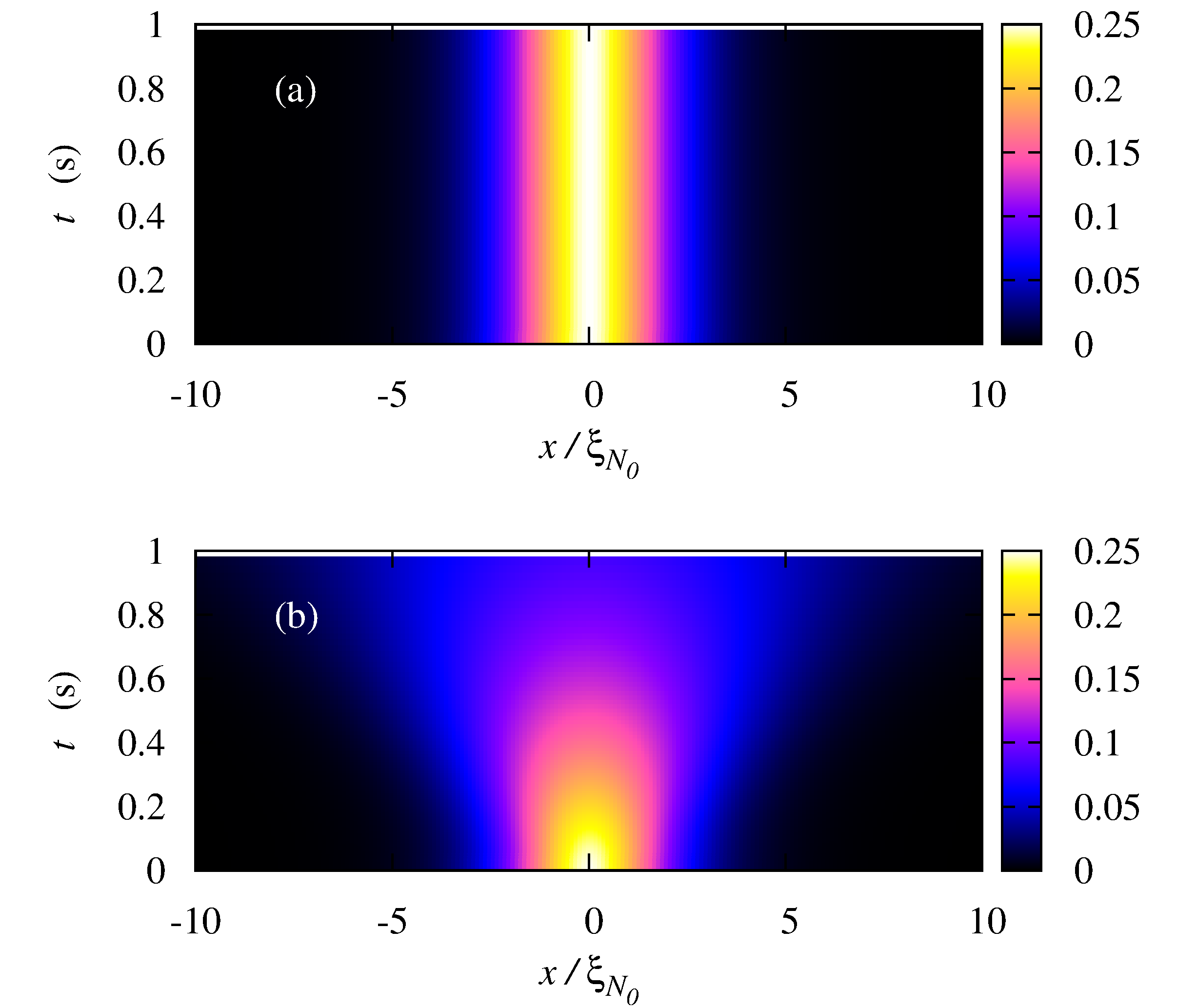
Figure 1 shows the influence of the center-of-mass position on the single particle density of a quantum bright soliton of Li atoms (as experimentally investigated at high velocities in KhaykovichEtAl2002 ). The GPE soliton remains stationary [Fig. 1 (a)]; that is, the single particle density is given by Eq. (2) for all times. Figure 1 (b) displays the same situation as panel (a) but for a quantum bright soliton for which the center-of-mass wave function spreads according to Eq. (7). Thus, for a quantum bright soliton we have a spreading single particle density – although each single measurement yields the mean-field soliton density [Fig. 1 (a)], shifted from the initial position by some distance.
For each single experiment, measuring the center-of-mass density of the many-particle configuration can be done with greater accuracy than the width of the cloud (cf. Ref. GertjerenkenWeiss2012 ). The expansion of the center-of-mass wave function leads to the spreading of the single particle density, in this paper we consider this spreading in the absence of harmonic trapping potentials. Recent experiments for homogeneous Bose gases can be found in Refs. GauntEtAl2013 ; SchmidutzEtAl2014 .
III Decoherence via three-particle losses
III.1 Three particle-losses
Three-particle losses can be described by a density-dependent rate equation GrimmEtAl2000 :
| (11) |
where is determined empirically. Combined with Eq. (10) and using the soliton length (3) this yields maple
| (12) |
with the -independent time scale:
| (13) |
For this equation to be valid at longer time-scales (and not just initially), the single particle density must remain of the form (10) as the width of the wave function in the -direction increases with decreasing particle number. We will show that this assumption is self-consistent, thus allowing us to treat atom losses as point processes (referring to points in time) within our stochastic approach.
III.2 Stochastic modeling of decoherence via three-particle losses
If changes to the number of particles in a soliton happen on slow enough time scales, these changes can be modeled as being adiabatic. The shape of the soliton is protected WeissCastin2009 (cf. HelmEtAl2014 ) by an energy gap
| (16) |
where is the ground state energy McGuire1964 of a system of 1D point bosons of mass interacting via attractive delta interactions, described by the Lieb-Liniger Hamiltonian (8).
The energy-time uncertainty yields a characteristic time scale (cf. HoldawayEtAl2012 ) via , where
| (17) |
Changes in particle numbers should happen on time scales longer than this time for the process to be adiabatic, and for our approach of treating particle losses as an adiabatic process to be valid. So far, three-particle losses in experiments have not been observed to destroy solitons on short time scales KhaykovichEtAl2002 . We can thus model the particle losses as taking place on time scales longer than the soliton time if the soliton time is smaller than the time scale on which a single particle is lost, that is,
| (18) |
With and the experimental parameters of KhaykovichEtAl2002 222The set of parameters used as an example to show that experimentally realistic time scales uses the values given in Ref. KhaykovichEtAl2002 for the s-wave scattering length , where . For this s-wave scattering length we furthermore divide the calculated value ShotanEtAl2014 for the thermal of by the factor for Bose-Einstein condensates and (thus also bright solitons).
| (19) |
The inequality (18) is fulfilled for the parameters of KhaykovichEtAl2002 if . We can furthermore model the three-particle losses as taking place instantaneously for our stochastic implementation DalibardEtAl1992 ; DumEtAl1992 ; Breuer2006 of particle losses.
For a Schrödinger cat state HarocheRaimond2006 , a quantum superposition of two “macroscopically” occupied single particle modes, 333The tensor product power notation describes particles occupying the same single-particle mode ., losing three particles leads to a localization in one of the two modes, or . Quantum bright solitons are in a spatial quantum superposition given by their center-of-mass wave function; if the center-of-mass wave function is a delta function, the wave function can be approximated by a Hartree-product state consisting of occupying the mean-field (GPE) wave function times CastinHerzog2001 . We thus will model the collapse of the wave function into one of these modes as a starting point to describe the influence of decoherence via three-particle losses on the center-of-mass motion of quantum bright solitons.
We can use the Schrödinger equation for a single particle of mass with Hamiltonian to describe the quantum mechanical motion of the center of mass of a quantum bright soliton in the absence of decoherence events WeissCastin2009 . Note that the particle number remains constant between loss events.
For the internal degrees of freedom, we can use a Hartree-product-state PethickSmith2008 of bright-soliton solutions of the GPE (1),
| (20) |
with and . After the three particle loss, the internal degrees of freedom are described by the wave function given by Eq. (20) with replaced by . As we will describe below, both the position and the velocity (via the center-of-mass density) as well as the point of time for this decoherence [via Eq. (12)] are determined via random numbers in a Monte Carlo simulation. A characteristic size for the new center-of-mass wave function is the root-mean-square width of the soliton (cf. Appendix A)
| (21) |
In order to describe the stochastic process, we introduce an approach via a classical master equation. While at first glance this approach may seem to be impossible, as between loss events we have a purely quantum mechanical expansion of the center-of-mass wave function, the fact that our system can indeed be described by a classical model is justified below. Within our model the stochastic variables are given by the center of mass coordinate , the corresponding velocity and the particle number . Introducing the time-dependent probability distribution the stochastic process is defined by the master equation
| (22) |
The first term on the right-hand side describes the constant drift of with velocity while the second term represents the instantaneous random jumps induced by three-particle losses. The process is thus a piecewise deterministic process Davis1993 with transition rates
| (23) |
where is given by Eq. (21), and
The total transition rate takes the form
| (24) |
where we have added a factor of as three particles are lost each time. We thus have an exponential waiting time distribution
| (25) |
To summarize, for the stochastic simulation of decoherence via three-particle losses Breuer2006 , the ingredients are:
-
1.
The random variables:
(26) -
2.
Random numbers for the Monte-Carlo process determine:
- (a)
-
(b)
The center-of-mass position of the new wave function via the center-of-mass density in real space.
-
(c)
The center-of-mass velocity of the new wave function via the center-of-mass density in momentum space.
- 3.
In between loss events, the quantum dynamics is known analytically [Eq. (6)]; rather than solving the Schrödinger equation it is possible to do this in a more classical approach: The truncated Wigner approximation 444The truncated-Wigner approximation SinatraEtAl2002 describes quantum systems by averaging over realizations of an appropriate classical field equation (in this case, the GPE) with initial noise appropriate to either finite BieniasEtAl2011 or zero temperatures MartinRuostekoski2012 . for the center of mass, which has been used in Ref. GertjerenkenEtAl2013 to qualitatively mimic quantum behavior on the mean-field level by introducing classical noise mimicking the quantum uncertainties in both position and momentum, is particularly useful here: both the mean position and the variance calculated via the Truncated Wigner Approximation for the center of mass are identical to the quantum mechanical result. In order to make both results identical, Gaussian noise has to be added independently to both position and velocity with and and root-mean-square fluctuations given by Eq. (28) and by the minimal uncertainty relation
| (29) |
for the velocity.
The mean position is thus identical to the quantum mechanical result; the root-mean-square fluctuations coincide with the quantum mechanical equation (7). Thus, in the absence of both the trap in the axial direction and the scattering processes investigated in Ref. GertjerenkenEtAl2013 , the TWA for the center of mass gives exact results for both the position of the center of mass and the root-mean-square fluctuations of the center of mass for a quantum bright soliton.
IV Results
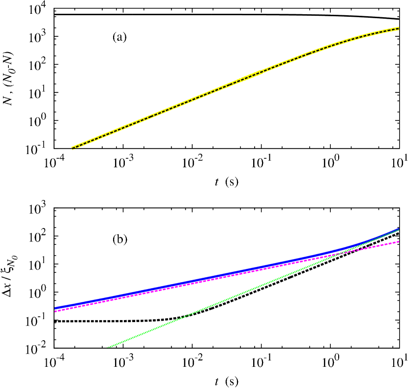
Figure 2 shows the influence of decoherence via three-particle losses on the center-of-mass displacement of quantum bright solitons made out of Li atoms for parameters taken from the experiment KhaykovichEtAl2002 (see footnote 2). Three-particle losses, which could only be prevented by considerably reducing the density of a bright soliton to values much lower than used in experiments such as KhaykovichEtAl2002 , and are thus a decoherence mechanism intrinsic to quantum bright solitons, lead to a transition from short-time diffusive to long-time ballistic behavior [Fig. 2 (b)]. The numerical simulations were done by using the piece-wise deterministic processes Davis1993 described in Sec. III.2, a well-established tool to model decoherence DalibardEtAl1992 ; DumEtAl1992 ; Breuer2006 .
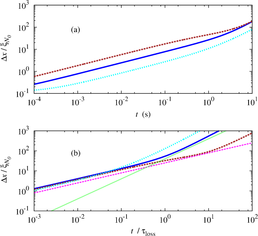
Figure 3 shows that the transition from short-time diffusive to long-time ballistic behavior is not dependent on a particular choice of parameters. While details of the curves can look different for different parameters, the transition from short-term diffusive to long-time ballistic behavior is visible in particular after rescaling the time-axis with the characteristic time-scale given by the atom losses [Eq. (14)]; thus using the scaling for which all curves would lie on top of each other. Within this scaling, all curves follow the same scaling for early scaled times, and they each start deviating off at different times.
This scaling leads to an intuitive explanation of the transition from short-time diffusive to long-time ballistic motion. While the atom losses continue in the regime of ballistic motion [as can be seen by comparing panels (a) and (b) of Fig. 2], is the time-scale on which starts to forget its initial number of particles. In addition, the center-of-mass motion also picks up pace for longer time-scales. As the Gross-Pitaevskii equation (GPE) becomes valid in the limit , such that the product remains constant LiebEtAl2000 , it cannot model an expanding center-of-mass wave function. Thus, the transition from short-time ballistic to long-time diffusive behavior cannot be modeled by simply using standard GPE-theory.
V Conclusion and outlook
To conclude, we have introduced a physically motivated model for the motion of quantum bright solitons which displays short-time diffusive and long-time ballistic behavior, contrary to the usual short-time ballistic and long-time diffusive behavior observed for example in Brownian motion LukicEtAl2005 . Bright solitons are investigated experimentally in various groups world-wide. As the ballistic expansion for large times is [Eq. (7)] the solitons made of thousands of Li atoms KhaykovichEtAl2002 are more suitable to observe this motion of the center-of-mass than solitons made of thousands of the more than ten times heavier Rb atoms MarchantEtAl2013 . For the ground-state atoms of Li used, for example, in the ground-breaking experiments KhaykovichEtAl2002 ; StreckerEtAl2002 there are no two-body losses GrimmEtAl2000 ; single-particle losses can also be discounted if the vacuum is made to be particularly good (cf. AndersonEtAl1995 ). Our approach to focus on decoherence via three-particle losses to model matter-wave bright solitons in attractive Li-Bose-Einstein condensates thus is justified.
The present idea to modify the quantum mechanical motion by stochastic terms in order to describe instantaneous changes of the wave function to smaller wave packets has formal similarities with stochastic collapse models GhirardiEtAl1986 . However, within our model these random changes describe the decoherence of the center-of-mass wave function which is induced by three-particle losses; a decoherence mechanism which cannot be avoided by, e.g., choosing a perfect vacuum: as long as the density is finite (which always is the case for bright solitons), three-particle losses will occur as a dominant decoherence mechanism. It is the decrease of the particle number that leads to fewer particle losses and, hence, to the observed transition from diffusive to ballistic motion. This motion is an effect distinct from both classical Metzler2000 and quantum walks cf. DurEtAl2002 ; KarskiEtAl2009 as well as anomalous diffusion Metzler2000 ; SiemsEtAl2012 ; TurivEtAl2013 . As for the classical random walk, our model localizes after each step, but between steps the motion is given by free expansion of the center-of-mass wave function which depends on the (decreasing) number of particles.
This unusual behavior of the center-of-mass motion can be observed for experimentally realistic parameters; both time scales and length scales are accessible experimentally.
Acknowledgements.
We thank S. L. Cornish, S. A. Hopkins and L. Khaykovich for discussions. C.W. thanks the Institute of Physics, University of Freiburg, for its hospitality. We thank the UK Engineering and Physical Sciences Research Council (Grant No. EP/L010844/1, C.W. and S.A.G.) for funding. The data presented in this paper are available from http://dx.doi.org/10.15128/kk91fk954.Appendix A Size of Center-of-Mass wave function after collapse
The focus of this paper was to present a physically motivated model which displays a transition from short-time diffusive to long-time ballistic behavior. Time-scales can easily be changed by, e.g., choosing a trapping geometry different from the parameters used in Ref. KhaykovichEtAl2002 . The focus currently is on a macroscopic theory; for future microscopic theories some details like the center-of-mass wave function after a decoherence-event via the physically dominating decoherence mechanism, a three-particle loss-event, might differ from the value chosen here. In order to show that the transition from diffusive to ballistic behavior would still be observable for other choices of the width of the center-of-mass wave function, Fig. 4 displays the behavior for
| (30) |
This corresponds to the idealized case that the wave function collapses to a single product state (20), the root-mean-square width of the new center-of-mass wave function of the soliton consisting of particles is given by the prediction of the central limit theorem (cf. HoldawayEtAl2012 )
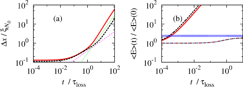
Figure 4 shows, that as for the choice in the main part of the paper, for Eq. (30) the combined effect of the rate of particle losses decreasing and becoming more independent of [cf. Eq. (14)] and the center-of-mass motion covering greater distances leads again to a transition from short-time diffusive to long-time ballistic behavior. However, contrary to the case discussed in the main part of the paper, the kinetic energy is considerably increased during the motion. While the open system discussed in this paper could include such a mechanism, unless experimental results should oblige one to introduce such a mechanism, the model presented in the main part of the paper is the more physical choice.
References
- (1) J. S. Russell, In Report of the Fourteenth Meeting of the British Association for the Advancement of Science 311–390 (John Murray)(1845)
- (2) L. Khaykovich, F. Schreck, G. Ferrari, T. Bourdel, J. Cubizolles, L. D. Carr, Y. Castin, and C. Salomon, Science 296, 1290 (2002)
- (3) K. E. Strecker, G. B. Partridge, A. G. Truscott, and R. G. Hulet, Nature (London) 417, 150 (2002)
- (4) S. L. Cornish, S. T. Thompson, and C. E. Wieman, Phys. Rev. Lett. 96, 170401 (2006)
- (5) A. L. Marchant, T. P. Billam, T. P. Wiles, M. M. H. Yu, S. A. Gardiner, and S. L. Cornish, Nat. Commun. 4, 1865 (2013)
- (6) P. Medley, M. A. Minar, N. C. Cizek, D. Berryrieser, and M. A. Kasevich, Phys. Rev. Lett. 112, 060401 (2014)
- (7) G. D. McDonald, C. C. N. Kuhn, K. S. Hardman, S. Bennetts, P. J. Everitt, P. A. Altin, J. E. Debs, J. D. Close, and N. P. Robins, Phys. Rev. Lett. 113, 013002 (2014)
- (8) J. H. V. Nguyen, P. Dyke, D. Luo, B. A. Malomed, and R. G. Hulet, Nature Phys. 10, 918 (2014)
- (9) C. J. Pethick and H. Smith, Bose-Einstein Condensation in Dilute Gases (Cambridge University Press, Cambridge, 2008)
- (10) B. B. Baizakov, V. V. Konotop, and M. Salerno, J. Phys. B 35, 5105 (2002)
- (11) U. Al Khawaja, H. T. C. Stoof, R. G. Hulet, K. E. Strecker, and G. B. Partridge, Phys. Rev. Lett. 89, 200404 (2002)
- (12) W. Hai, C. Lee, and G. Chong, Phys. Rev. A 70, 053621 (2004)
- (13) A. D. Martin and J. Ruostekoski, New J. Phys. 14, 043040 (2012)
- (14) J. L. Helm, T. P. Billam, and S. A. Gardiner, Phys. Rev. A 85, 053621 (2012)
- (15) J. Cuevas, P. G. Kevrekidis, B. A. Malomed, P. Dyke, and R. G. Hulet, New J. Phys. 15, 063006 (2013)
- (16) J. Polo and V. Ahufinger, Phys. Rev. A 88, 053628 (2013)
- (17) Y. Lai and H. A. Haus, Phys. Rev. A 40, 854 (1989)
- (18) P. D. Drummond, R. M. Shelby, S. R. Friberg, and Y. Yamamoto, Nature (London) 365, 307 (1993)
- (19) L. D. Carr and J. Brand, Phys. Rev. Lett. 92, 040401 (2004)
- (20) A. I. Streltsov, O. E. Alon, and L. S. Cederbaum, Phys. Rev. Lett. 106, 240401 (2011)
- (21) T. Fogarty, A. Kiely, S. Campbell, and T. Busch, Phys. Rev. A 87, 043630 (2013)
- (22) D. Delande, K. Sacha, M. Płodzień, S. K. Avazbaev, and J. Zakrzewski, New J. Phys. 15, 045021 (2013)
- (23) B. Gertjerenken, T. P. Billam, C. L. Blackley, C. R. Le Sueur, L. Khaykovich, S. L. Cornish, and C. Weiss, Phys. Rev. Lett. 111, 100406 (2013)
- (24) L. Barbiero and L. Salasnich, Phys. Rev. A 89, 063605 (2014)
- (25) J. B. McGuire, J. Math. Phys. 5, 622 (1964)
- (26) F. Calogero and A. Degasperis, Phys. Rev. A 11, 265 (1975)
- (27) Y. Castin and C. Herzog, C. R. Acad. Sci. Paris, Ser. IV 2, 419 (2001), arXiv:cond-mat/0012040
- (28) E. H. Lieb and W. Liniger, Phys. Rev. 130, 1605 (1963)
- (29) I. E. Mazets and G. Kurizki, EPL (Europhys. Lett.) 76, 196 (2006)
- (30) G. E. Uhlenbeck and L. S. Ornstein, Phys. Rev. 36, 823 (Sep. 1930)
- (31) H. Grabert, P. Schramm, and G.-L. Ingold, Phys. Rep. 168, 115 (Oct. 1988)
- (32) P. Jung and P. Hänggi, Phys. Rev. A 44, 8032 (1991)
- (33) G. M. Wang, E. M. Sevick, E. Mittag, D. J. Searles, and D. J. Evans, Phys. Rev. Lett. 89, 050601 (2002)
- (34) B. Lukić, S. Jeney, C. Tischer, A. J. Kulik, L. Forró, and E.-L. Florin, Phys. Rev. Lett. 95, 160601 (2005)
- (35) M. Köppl, P. Henseler, A. Erbe, P. Nielaba, and P. Leiderer, Phys. Rev. Lett. 97, 208302 (2006)
- (36) T. Ando and J. Skolnick, Proc. Natl. Acad. Sci. 107, 18457 (2010)
- (37) R. Steinigeweg, H.-P. Breuer, and J. Gemmer, Phys. Rev. Lett. 99, 150601 (2007)
- (38) R. Metzler and J. Klafter, Phys. Rep. 339, 1 (2000)
- (39) U. Siems, C. Kreuter, A. Erbe, N. Schwierz, S. Sengupta, P. Leiderer, and P. Nielaba, Sci. Rep. 2, 1015 (2012)
- (40) T. Turiv, I. Lazo, A. Brodin, B. I. Lev, V. Reiffenrath, V. G. Nazarenko, and O. D. Lavrentovich, Science 342, 1351 (2013)
- (41) R. Metzler and J. Klafter, J. Phys. A: Math. Gen. 37, R161 (2004)
- (42) D. Dries, S. E. Pollack, J. M. Hitchcock, and R. G. Hulet, Phys. Rev. A 82, 033603 (2010)
- (43) S. Sinha, A. Y. Cherny, D. Kovrizhin, and J. Brand, Phys. Rev. Lett. 96, 030406 (2006)
- (44) C. Weiss and Y. Castin, Phys. Rev. Lett. 102, 010403 (2009)
- (45) R. Grimm, M. Weidemüller, and Y. B. Ovchinnikov, Adv. At. Mol. Opt. Phys. 42, 95 (2000), physics/9902072
- (46) M. H. Anderson, J. R. Ensher, M. R. Matthews, C. E. Wieman, and E. A. Cornell, Science 269, 198 (1995)
- (47) M. H. A. Davis, Markov models and optimization (Chapman & Hall, London, 1993)
- (48) M. Olshanii, Phys. Rev. Lett. 81, 938 (1998)
- (49) Y. Castin, Eur. Phys. J. B 68, 317 (2009)
- (50) M. Bonitz, K. Balzer, and R. van Leeuwen, Phys. Rev. B 76, 045341 (2007)
- (51) B. Gertjerenken, Phys. Rev. A 88, 053623 (2013)
- (52) S. Flügge, Rechenmethoden der Quantentheorie (Springer, Berlin, 1990)
- (53) E. H. Lieb, R. Seiringer, J. P. Solovej, and J. Yngvason, Current Developments in Mathematics, 2001, 131(2002)
- (54) B. Gertjerenken and C. Weiss, Phys. Rev. A 88, 033608 (2013)
- (55) B. Gertjerenken and C. Weiss, J. Phys. B 45, 165301 (2012)
- (56) A. L. Gaunt, T. F. Schmidutz, I. Gotlibovych, R. P. Smith, and Z. Hadzibabic, Phys. Rev. Lett. 110, 200406 (2013)
- (57) T. F. Schmidutz, I. Gotlibovych, A. L. Gaunt, R. P. Smith, N. Navon, and Z. Hadzibabic, Phys. Rev. Lett. 112, 040403 (2014)
- (58) Computer algebra programme Maple
- (59) J. L. Helm, S. J. Rooney, C. Weiss, and S. A. Gardiner, Phys. Rev. A 89, 033610 (2014)
- (60) D. I. H. Holdaway, C. Weiss, and S. A. Gardiner, Phys. Rev. A 85, 053618 (2012)
- (61) Z. Shotan, O. Machtey, S. Kokkelmans, and L. Khaykovich, Phys. Rev. Lett. 113, 053202 (2014)
- (62) J. Dalibard, Y. Castin, and K. Mølmer, Phys. Rev. Lett. 68, 580 (1992)
- (63) R. Dum, P. Zoller, and H. Ritsch, Phys. Rev. A 45, 4879 (1992)
- (64) H.-P. Breuer and F. Petruccione, The Theory of Open Quantum Systems (Clarendon Press, Oxford, 2006)
- (65) S. Haroche and J.-M. Raimond, Exploring the Quantum – Atoms, Cavities and Photons (Oxford University Press, Oxford, 2006)
- (66) A. Sinatra, C. Lobo, and Y. Castin, J. Phys. B 35, 3599 (2002)
- (67) P. Bienias, K. Pawlowski, M. Gajda, and K. Rzazewski, EPL (Europhys. Lett.) 96, 10011 (2011)
- (68) E. H. Lieb, R. Seiringer, and J. Yngvason, Phys. Rev. A 61, 043602 (2000)
- (69) G. C. Ghirardi, A. Rimini, and T. Weber, Phys. Rev. D 34, 470 (1986)
- (70) W. Dür, R. Raussendorf, V. M. Kendon, and H.-J. Briegel, Phys. Rev. A 66, 052319 (2002)
- (71) M. Karski, L. Förster, J.-M. Choi, A. Steffen, W. Alt, D. Meschede, and A. Widera, Science 325, 174 (2009)