Space-Based Cosmic-Ray and Gamma-Ray Detectors: a Review

Abstract

Prepared for the 2014 ISAPP summer school, this review is focused on space-borne and balloon-borne cosmic-ray and gamma-ray detectors. It is meant to introduce the fundamental concepts necessary to understand the instrument performance metrics, how they tie to the design choices and how they can be effectively used in sensitivity studies. While the write-up does not aim at being complete or exhaustive, it is largely self-contained in that related topics such as the basic physical processes governing the interaction of radiation with matter and the near-Earth environment are briefly reviewed.

I Prelude

This write-up was prepared for the ISAPP School “Multi-wavelength and multi-messenger investigation of the visible and dark Universe held in Belgirate between 21 and 30 July 2014. As such the reader should not expect it to be accurate and/or terse as an actual scientific publication. It is largely idiosyncratic and guaranteed to contain errors, instead.

That said, this review might be expanded and/or improved in the future, depending on whether people will find it useful or not. If you find a mistake or you have suggestions, do not hesitate to inform the author—though you should not expect him to be working on this project with a significant duty cycle, nor necessarily proactive. (Note, however, that I am committed to fix right away any instance where the work of individuals or research groups has arguably been misrepresented.)

I.1 Overview

The main focus of this review is introducing the basic instrument performance metrics, with emphasis on space-born and balloon-borne cosmic-ray and gamma-ray detectors. While, in general, instrument response functions can only be predicted accurately by means of detailed Monte Carlo simulations, the main features can be typically understood (say within a factor of two) by means of simple, back-of-envelope calculations based on the micro-physics of the particle interaction in the detector. Such an approach is effective in highlighting the connection between the underlying design choices and the actual instrument sensitivity.

To give some context to the discussion, the current body of knowledge on cosmic and gamma rays is briefly reviewed in historical prospective, and the basics of interactions between radiation and matter, along with the main characteristics of the near-Earth environment, are concisely covered. A honest attempt has been made to provide a complete and up-to date list of references to the relevant sources in the literature.

The organization of the material is not necessarily the most natural one, based on the consideration that, if we were to write it down in strict logical order, deriving each fact from the prime principles, it is unlikely that the average reader would get past page 2. Instead, we frequently switch back and forth and use concepts that, strictly speaking, are only introduced later in the flow of the discussion. We put some effort, though, in trying to provide explicit cross references between the different bits in a sensible way.

In the attempt to make it useful and—more importantly—usable, all the material contained in this review is copylefted under the GPL General Public License and available at https://bitbucket.org/lbaldini/crdetectors. This includes: the LaTeX source code, the tables, high-resolution versions of all the figures and the code (along with the necessary auxiliary data files) used to generate them.

II Introduction

The discovery of cosmic rays (CR) is customarily attributed to Viktor Franz Hess, who first demonstrated in a series of pioneering balloon flights performed in 1911 and 1912 that the ionizing radiation in the atmosphere of the Earth was of extraterrestrial origin. More than 100 years after their discoveries, cosmic rays have been extensively studied, both with space-based detectors and with ground observatories. For reference, the cosmic-ray database described in Maurin et al. (2013), which we have extensively used in the preparation of this review, contains some $\sim 1100$ data sets from $\sim 40$ different experiments at energies below $\sim 10^{15}$ eV.

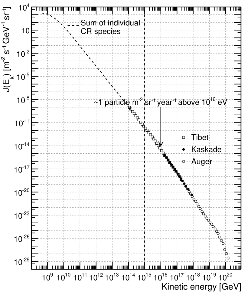
Figure 1: All-particle energy spectrum of primary cosmic rays, compiled from some of the most recent available measurements. The dashed line extending from $\sim 10^{9}$ to $\sim 10^{14}$ eV has been obtained by summing up the energy spectra of the most abundant CR species (p, He, C, O and Fe), measured by several different space- and balloon-borne experiments. The vertical dashed line marks the maximum energy ($\sim 1$ PeV) that can be practically measured by a CR detector in orbit.

Figure 1 provides a largely incomplete, and yet impressive, account of the tremendous body of knowledge that we have accumulated along the way. The dashed line extending from $\sim 10^{9}$ to $\sim 10^{14}$ eV is a weighted sum of the energy spectra of the most abundant CR species (p, He, C, O and Fe), as measured by several different space- and balloon-borne experiments. The reader is referred to Beringer et al. (2012) and references therein for a more comprehensive compilation of the available all-particle ultra-high energy cosmic-ray (UHECR) spectral measurements.

The immediate overall picture is that of a seemingly featureless power law extending over some $12$ orders of magnitude in energy and $33$ orders of magnitude in flux. As a matter of fact, cosmic-ray spectra are customarily weighted by some power of the energy (typically ranging from $2$ to $3$) in order to make relatively subtle intrinsic features more prominent—which is a fairly sensible thing to do, as those features are connected with the underlying physics. If we did so in this case, we would see the so-called knee emerging at a few $10^{15}$ eV, a second knee at $\sim 10^{18}$ eV, the ankle even higher energies and a spectral steepening, possibly to be interpreted as the GZK cutoff, around $10^{20}$ eV.

Here we shall take a slightly different perspective and start by noting that $10^{16}$ eV is roughly the energy where the integral all-particle cosmic-ray spectrum amounts to $\sim 1$ m^-2 sr^-1 year^-1. If we forget for a second the steradians (we shall see in section IX.2.1 that this essentially gives an extra factor of $\pi$, which is largely irrelevant for the purpose of our argument) this means that far away from the Earth there is about $1$ particle per year above $10^{16}$ eV crossing any $1$ m² plane surface. Now, $1$ m² is a large figure by any space-experiment standard—and $1$ year is not short either. This basic consideration naturally set the PeV scale as the upper limit to the energies than can be practically studied in space. It is fortunate that, though the atmosphere of the Earth is opaque to primary particles above $\sim 10$ eV, ultra-high-energy cosmic rays can be effectively studied from the ground through a variety of experimental techniques involving the detection of their secondary products—most notably the water-Cherenkov and florescence techniques, both exploited by the Pierre Auger Observatory Abraham et al. (2004), and the extensive air shower arrays a la KASKADE Antoni et al. (2003) or ARGO-YBJ Aielli et al. (2012). This is also true for high-energy gamma rays (above $\sim 100$ GeV), with at least three major advanced imaging Cherenkov telescopes operating at the time of writing (H.E.S.S., MAGIC, VERITAS) and the HAWC water-Cherenkov gamma-ray observatory currently under construction. We note, in passing, that the dichotomy between space-borne (or balloon-borne) and ground-based experiments has an important implication in that, while the former provide measurements of separate cosmic-ray species, for the latter it is much harder to infer the chemical composition. Important as it is, the synergy between ground- and space-base observatories will not be discussed further in this write-up.

At the other extreme of the energy spectrum (say below a few GeV), primary cosmic rays are heavily influenced by the heliospheric environment and reprocessed by the atmosphere and the magnetic field of the Earth. While the study of very low-energy primaries and of the geomagnetically trapped radiation is by no means less interesting than that of their higher-energy fellows, an informed discussion would require a large additional body of background information and is therefore outside the scope of the paper.

In broad terms, this review is focused on the seven energy decades between $\sim 100$ MeV and $1$ PeV—and particularly on the experimental techniques that have been (and are being) exploited to study cosmic rays and gamma rays in this energy range. The subject is well defined and homogeneous enough—both in terms of science topics and as far as experimental techniques are concerned—that it can be usefully discussed in a unified fashion.

III Basic formalism and notation

A significant part of cosmic-ray physics is about energy spectra. That said, you should be wary when you happen to hear a cosmic-ray physicist pronouncing the word spectrum: it might indicate all sort of things. On the $x$-axis you might find the particle (total or kinetic) energy, the energy per nucleon, the momentum or the rigidity. On the $y$-axis you might find a differential or integral flux or intensity, possibly multiplied by a power of the variable plotted on the $x$-axis. We shall not refrain ourselves from using the term spectrum in this somewhat loose sense, and the reader is advised that sometimes it’s pretty easy to get confused—so always pay attention to the axis labels!

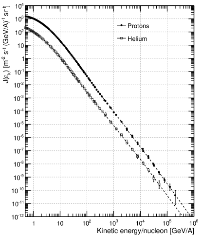
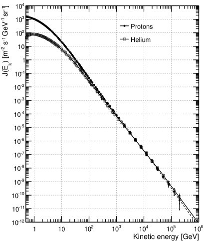
Figure 2: Differential intensities, plotted as a function of kinetic energy per nucleon (left) and total kinetic energy (right) for the two most abundant CR species: protons and He nuclei. While the He intensity is a factor of $\sim 10$ smaller than that of protons at, say, $\sim 1$ TeV/nucleon, the two are comparable, at $\sim 1$ TeV, when binned in total kinetic energy. See next section for more details about the data points and the dashed lines.

As a mere illustration, figure 2 shows how the proton and helium spectra look different, relative to each other, depending on whether the differential intensity is plotted as a function of the kinetic energy per nucleon or the total kinetic energy. We note, in passing, that the first choice is the one customarily adopted in this energy range and, clearly, the one that we have in mind when we make statements such as “protons account for $\sim 90\%$ of cosmic-rays”. That said, the second representation is not necessarily less meaningful—e.g., when dealing with the energy measurement in a calorimetric experiment. We’ll come back to this shortly.

In this section we introduce some basic terminology and notation that we shall use in the following.

Symbol	Description	Units
$Z$	Atomic number	–
$A$	Mass number	–
$\varrho$	Density	[${\rm g~{}cm}^{-3}$]
$\chi$	Grammage	[${\rm g~{}cm}^{-2}$]
$E$	Energy	[GeV]
$E_{\rm k}$	Kinetic energy	[GeV]
$\mathcal{E}_{\rm k}$	Kinetic energy/nucleon	[GeV/$A$]
$p$	Momentum	[GeV/c]
$R$	Rigidity	[GV]
$F$	Differential flux	[${\rm m}^{-2}~{}{\rm s}^{-1}~{}{\rm GeV}^{-1}$]
$J$	Differential intensity	[${\rm m}^{-2}~{}{\rm s}^{-1}~{}{\rm GeV}^{-1}~{}{\rm sr}^{-1}$]
		[${\rm m}^{-2}~{}{\rm s}^{-1}~{}({\rm GeV}/A)^{-1}~{}{\rm sr}^{-1}$]
$\delta$	Dipole anisotropy	–

Table 1: Summary table of some useful quantities, along with the corresponding symbols and measurement units we shall use throughout this write-up.

III.1 Fluxes and Intensities

The term (differential) flux indicates the number of particles per unit time and energy crossing the unit vector area toward a given direction in the sky and is customarily measured in ${\rm m}^{-2}~{}{\rm s}^{-1}~{}{\rm GeV}^{-1}$. We shall indicate differential fluxes with $F$ throughout this manuscript.

The concept of differential flux essentially applies to point source studies, where the incoming particles all arrive from the same direction. On the other hand, an isotropic flux of charged particles or photons is more conveniently characterized by its intensity $J$ (number of particles per unit time, energy, area and solid angle) which is typically measured in ${\rm m}^{-2}~{}{\rm s}^{-1}~{}{\rm GeV}^{-1}~{}{\rm sr}^{-1}$.

The distinction between differential fluxes and intensities is connected with the dispersive nature of gamma-ray astronomy—in gamma rays you observe a different patch of the sky at any time, while cosmic rays are approximately the same in all directions. As we shall see in section IX, the consequences are far reaching in terms of describing the instrumental sensitivity. We shall try and stick to this nomenclature religiously throughout the manuscript.

Sometimes it is handy to work with quantities related to the number of events detected above a given energy—integral fluxes and intensities are useful concepts that will be widely used in the following.

Depending on the situation, differential and integral fluxes and intensities can be expressed as a function of energy, energy per nucleon, momentum and rigidity. Trivial as this might seem, there is a few subtleties involved in the conversion between different representation that we shall discuss in the next section.

III.2 Energy, momentum and all that

The total energy $E$, kinetic energy $E_{\rm k}$ and momentum $p$ of a particle or nucleus are related to each other (through the rest mass $m$) by the well known relativistic formulæ

$$p =mc\beta\gamma$$ (1)

$$E^{2} =m^{2}c^{4}+p^{2}c^{2}$$ (2)

$$E_{\rm k} =E-mc^{2},$$ (3)

that allow to switch from one variable to another when needed. When dealing with ultra-relativistic particles (i.e., when $E\gg mc^{2}$, which is not uncommon at all, in this context) energy, kinetic energy and momentum are really the same thing—modulo the speed of light $c$—and one does not need to bother about the differences. But for, e.g., protons and heavier nuclei below $\sim 10$ GeV the spectra do look different depending on the variable they are binned in (see figure 2).

Since we are at it, here is a few other relativistic formulæ that we shall occasionally use in the following—they express $\beta$, $\gamma$ and $\beta\gamma$ as a function of momentum, total energy and kinetic energy:

$$\beta =\frac{pc}{\sqrt{m^{2}c^{4}+p^{2}c^{2}}}=\sqrt{1-\frac{m^{2}c^{4}}{{E}^{2}}}=\frac{\sqrt{E_{\rm k}^{2}+2E_{\rm k}mc^{2}}}{E_{\rm k}+mc^{2}}$$ (4)

$$\gamma =\sqrt{1+\frac{p^{2}c^{2}}{m^{2}c^{4}}}=\frac{E}{mc^{2}}=1+\frac{E_{\rm k}}{mc^{2}}$$ (5)

$$\beta\gamma =\frac{p}{mc}=\sqrt{\frac{{E}^{2}}{m^{2}c^{4}}-1}=\sqrt{\frac{{E_{\rm k}}^{2}+2E_{\rm k}mc^{2}}{m^{2}c^{4}}}.$$ (6)

The rigidity $R$ is essentially the ratio between the momentum and the charge $Z$ (measured in units of the electron charge $e$) of a particle:

$$R=\frac{pc}{Ze}$$ (7)

Since we shall deal with magnetic fields—and it is easy to realize that particles with the same rigidity behave the same way in a magnetic field—this is a useful concept.

Finally, the CR spectra for He and heavier nuclei are more conveniently expressed as a function of the kinetic energy per nucleon

$$\mathcal{E}_{\rm k}=\frac{E_{\rm k}}{A}.$$ (8)

The kinetic energy per nucleon is a useful concept because, from the standpoint of the hadronic interactions, a nucleus with mass number $A$ and kinetic energy $E_{\rm k}$ behaves, to a large extent, as the superposition of $A$ nucleons with kinetic energy $E_{\rm k}/A$. (As a matter of fact, this is equally true—and relevant—in the interstellar medium, in the Earth atmosphere and in the calorimeter of a particle-physics detector.) It goes without saying that the kinetic energy per nucleon is conserved in spallation processes, and that it’s also the basic quantity determining whether a nucleus is relativistic or not (which is the reason why differential intensities for different charged species look more similar to each other in shape when binned in $\mathcal{E}_{\rm k}$).

Before we move on, we note that translating a differential intensity expressed in kinetic energy per nucleon into the same intensity expressed in (total) kinetic energy (or vice-versa) is slightly more complicated than scaling the $x$-axis by a factor $A$—one has also to scale the $y$-axis by a factor $1/A$, as by differential we really mean differential in whatever variable we have on the $x$-axis. If the original differential intensity is reasonably well described by a power-law with a spectral index $\Gamma$, a scale factor $A$ on the $x$-axis is equivalent to a factor $A^{\Gamma}$ on the $y$-axis and the whole thing is effectively equivalent to multiplying the data points by factor $A^{\Gamma-1}$:

$$J(E_{\rm k})\approx A^{\Gamma-1}J(\mathcal{E}_{\rm k}).$$ (9)

Is is not by chance that the two He spectra in figure 2 differ by a factor of $\sim 10$ in the high-energy regime, as $4^{1.75}\approx 10$.

III.3 Other observables

Charged-particle energy spectra (i.e. differential intensities) are not only interesting per se, but also in relation to each other. This aspect customarily goes under the name of cosmic-ray chemical composition, which is a crucial piece of information, as it probes the diffusion processes in the Galaxy and provides an indirect measurement of the material traversed by cosmic rays in their random walk from the source to the observer. The isotopical composition, accessible by magnetic spectrometers, is an interesting sub-chapter of this topic (more on this in section VIII.5.2).

On a related note, CR arrival directions generally bear no real memory of the source—except, possibly, for the highest energies (see, e.g., Lipari (2008)), which are not really of interest, in this context. Nonetheless the anisotropy on large angular scales is another interesting observable, especially for the leptons (since they rapidly loose energy due to radiation they probe the nearby galactic space). In the somewhat naïve scenario where the intensity is dominated by a single (nearby) source, one expects a dipole anisotropy by the Firck’s law. More generally, in a multipole analysis one could expect detectable signatures on medium to large scales due to the stochastic nature of the sources.

Anisotropies at all angular scales are also interesting in gamma rays, both in connection with the study of the galactic diffuse emission and the contribution of source populations to the extra-galactic diffuse emission.

As gamma rays do point back to their sources, the position and morphology of point/extended sources are yet other relevant observables. We shall come back to this later in the write-up.

We end the list mentioning the exciting perspective of measuring gamma-ray polarization in the pair production regime.

III.4 The grammage

When a particle traverses a homogeneous slab of a material—say some compressible gas at a given pressure—the average number of scattering centers it encounters is proportional to the product between the density $\varrho$ and the thickness $l$ of the slab. Doubling one and reducing the other by $1/2$ does not really change anything: the quantity characterizing the amount of material traversed is the grammage

$$\chi=\varrho l,$$ (10)

which is measured in g cm^-2 in the cgs system. This quantity is also referred to as the mass per unit area, as

$$\varrho=\frac{m}{V}=\frac{m}{lS},$$ (11)

and therefore

$$\chi=\frac{m}{S}.$$ (12)

There are many situations in which the grammage is a useful concept, e.g., in characterizing the integrated column density that cosmic rays traverse in their random walk from the source to the observer or the residual atmosphere at the typical balloon floating altitude. In both cases it is really the product of the density times the path length (or, more precisely, the integral of the density along the path, as the density is not constant) that matters.

The grammage is not the only quantity measured in g cm^-2 we shall encounter in the following. The radiation and interaction length of materials—as we shall see in sections VII.4 and VII.5 these are the typical length scales over which electromagnetic and hadronic showers develop—are customarily measured in the same units, as they tend to be smaller for denser material. In this case the mass scaling law is only approximate and measuring these quantities in ${\rm g~{}cm}^{-2}$ underlines the intrinsic differences. One can then recover the actual length scale (in cm) just dividing by the density. We shall see in section VI.1.3 how comparing the grammage and the radiation length in a variable-density environment (the atmosphere of the Earth) turns out to be handy.

IV Galactic cosmic rays

In order to give some context for the following discussion, in this section we briefly summarize some of the basic facts about galactic cosmic rays.

IV.1 The spectrum of galactic cosmic rays

The energy spectrum of individual CR species has now been measured by space- and balloon-borne detectors over some 7 decades in energy—at least for the more abundant ones—and is largely dominated by protons, as shown in figure 3. Among the other singly-charged species, electrons amount to some $10^{-2}$–$10^{-3}$ (depending on the energy) of the proton flux, and positrons and antiprotons are even less abundant, the latter being some $10^{-4}$ of the proton flux. We shall come back to these numbers in section IX.1 when discussing the challenges one has to face in separating the different species.

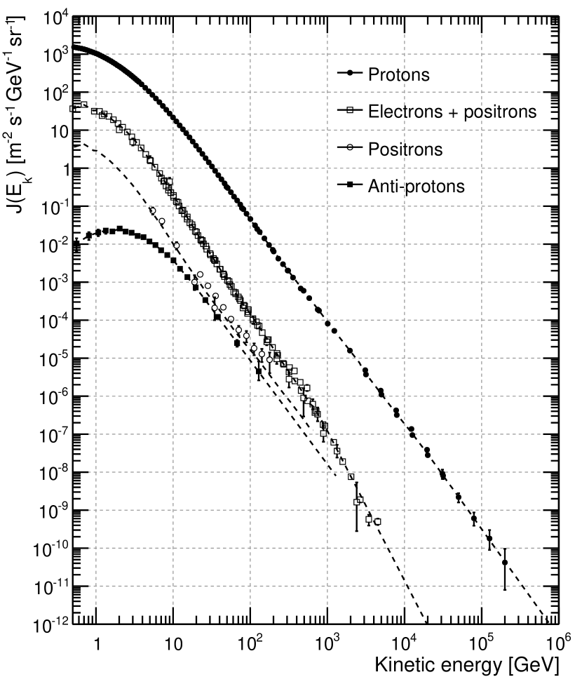
Figure 3: Spectra of the singly-charged components of the cosmic radiation. The data points are taken from Maurin et al. (2013) and correspond to references Panov et al. (2009); Yoon et al. (2011); Adriani et al. (2011a); Chang et al. (2008); Aharonian et al. (2008); Ackermann et al. (2010); Adriani et al. (2011b); Rastoin et al. (1996); Ackermann et al. (2012a); Barwick et al. (1998); Adriani et al. (2013a). For each species, the dashed line represents the weighted average of all the recent available measurements, and will be used in the following as the baseline for sensitivity estimates. For completeness, the model for the positron spectrum has been obtained by combining the $(e^{+}+e^{-})$ spectrum with the positron fraction measured by AMS-02 Aguilar et al. (2013).

As it turns out, cosmic rays include all sort of nuclei. Helium nuclei, amounting to some $10\%$ of the protons, constitute the second more abundant component, and carbon and oxygen are also relatively abundant, as shown in figure 4.

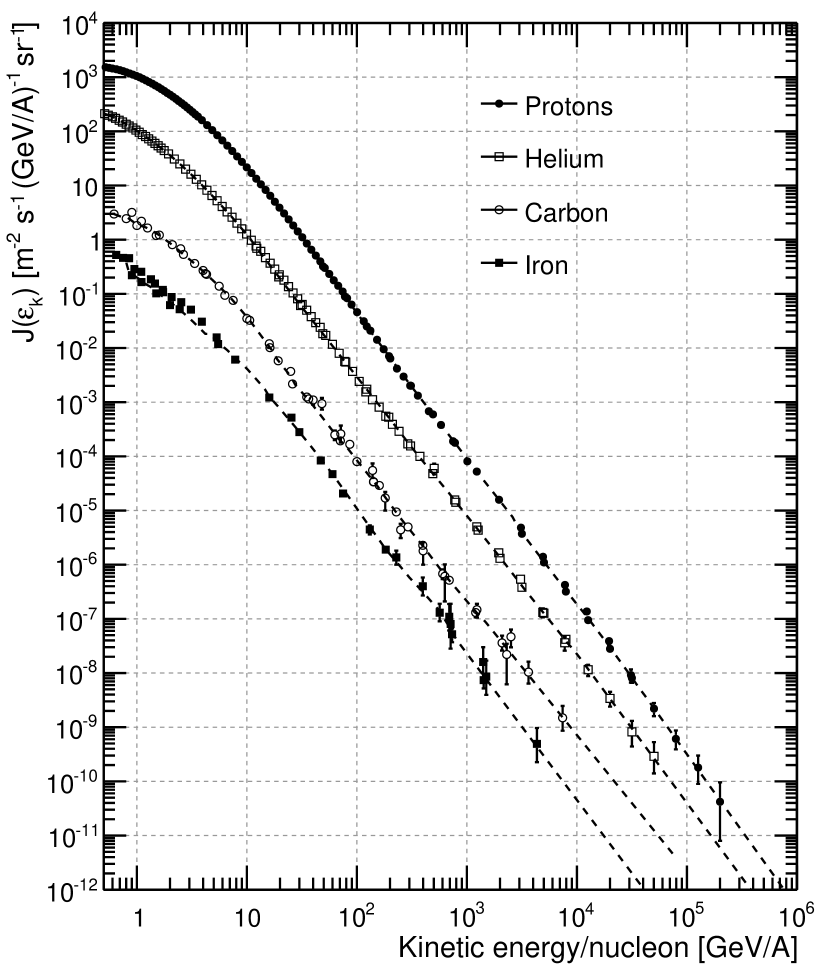
Figure 4: Spectra of some of the more abundant cosmic-ray species with $z>1$, compared with the proton spectrum shown in figure 3. The data points are taken from Maurin et al. (2013) and correspond to references Panov et al. (2009); Yoon et al. (2011); Adriani et al. (2011a); Ahn et al. (2009); Obermeier et al. (2011); Buckley et al. (1994); Simon et al. (1980); Engelmann et al. (1990); Ave et al. (2008); Derbina et al. (2005); Minagawa (1981); Young et al. (1981). For each species, the dashed line represents the weighted average of all the recent available measurements, and will be used in the following as the baseline for sensitivity estimates.

For completeness, the dashed lines in figures 3 and 4 represent weighted averages of all the recent available measurements for each CR species, and we shall use them in the rest of this review for sensitivity estimates. We shall be fairly liberal, within reason, in terms of extrapolating differential and integral spectra at energies where there are not yet measurements available.

Z	Element	Relative
		abundance
1	H	540
2	He	26
3–5	Li–Be	0.4
6–8	C–O	2.20
9–10	F–Ne	0.3
11–12	Na–Mg	0.22
13–14	Al–Si	0.19
15–16	P–S	0.03
17–18	Cl–Ar	0.01
19–20	K–Ca	0.02
21–25	Sc–Mn	0.05
26–28	Fe–Ni	0.12

Table 2: Relative abundances of several groups of cosmic-ray species at $10.6$ GeV/$A$ (adapted from Beringer et al. (2012)), normalized to that of oxygen ($3.29\times 10^{-2}$ ${\rm m}^{-2}~{}{\rm s}^{-1}~{}({\rm GeV}/A)^{-1}~{}{\rm sr}^{-1}$.

IV.2 The cosmic-ray gamma-ray connection

Though it is not very common to see cosmic-ray and gamma-ray differential intensities overlaid on the same plot, cosmic rays and gamma rays are tightly tied to each other. The vast majority of celestial gamma rays in the GeV energy range are produced by interactions of cosmic rays with the interstellar medium and with galactic magnetic and radiation fields. The study of this galactic diffuse emission provides a prospective on the diffusion of cosmic rays in the galaxy complementary to direct measurements—as a matter of fact, it is the realization that cosmic-ray interactions were bound to produce gamma rays that provided one of the earliest stimuli to the development of gamma-ray astronomy. On a slightly different note, since gamma rays do point back to their sources, they provide a direct view on the likely sources of cosmic rays—supernova remnnants (SNR). Finally, as we shall see in the following, the two fields of investigation share much in terms of experimental techniques.

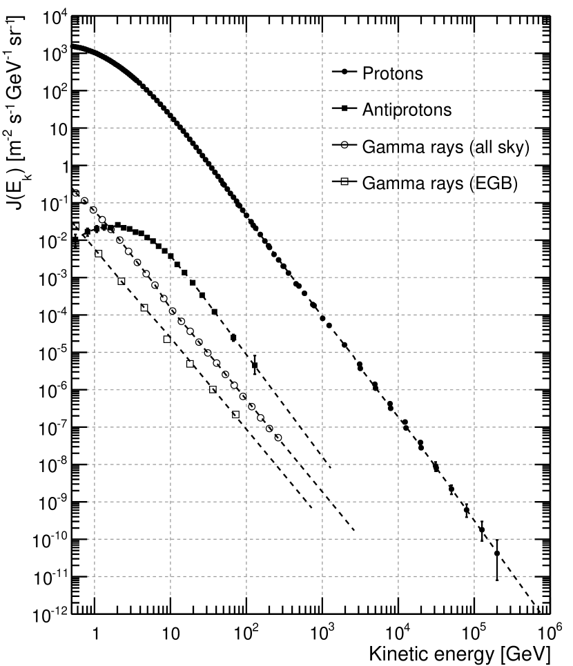
Figure 5: Energy spectrum of the all-sky gamma-ray intensity and of the extra-galactic gamma-ray background Abdo et al. (2010a), compared with the most and least abundant singly charged CR species (i.e., protons and antiprotons). Cosmic-ray data are taken from Maurin et al. (2013) and correspond to references Panov et al. (2009); Yoon et al. (2011); Adriani et al. (2011a); Ahn et al. (2009); Obermeier et al. (2011); Buckley et al. (1994); Simon et al. (1980); Engelmann et al. (1990); Ave et al. (2008); Derbina et al. (2005); Minagawa (1981); Young et al. (1981); Adriani et al. (2013a).

Figure 5 shows the all-sky gamma-ray differential intensity measured by the Fermi-LAT, and makes it fairly obvious that celestial gamma-rays constitute a tiny fraction of the cosmic radiation. Above $1$ GeV the entire gamma-ray sky intensity is more than an order of magnitude weaker than that of the rarest singly-charged species of the cosmic radiation—antiprotons—and five to six orders of magnitude less abundant than that of cosmic-ray protons. It goes without saying that the relative paucity of gamma-ray fluxes exacerbates the need for large instruments relative to charged species in the same energy range.

The difficulties in separating gamma rays out of the bulk of the charged cosmic-ray component are somewhat mitigated by the fact that efficient anticoincidence detectors can be realized to distinguish between neutral and charged particles and, at least for the analysis of gamma-ray sources, spatial—and sometimes temporal—signatures can be exploited. Nonetheless the measurement of the faint isotropic gamma-ray background may require a proton rejection factor as high as $10^{6}$. We shall discuss this in somewhat more details in section IX.1.

IV.3 The gamma-ray sky

In broad terms, the gamma-ray sky can be roughly subdivided in three main components: the galactic diffuse emission (DGE), point and extended sources, and the isotropic gamma-ray background (IGRB), sometimes referred as the extra-galactic background. In the next three subsections we shall briefly introduce these basic components.

IV.3.1 Galactic diffuse gamma-ray emission

As mentioned in the previous section, the vast majority of celestial gamma rays above 1 GeV are produced by the interaction of charged cosmic rays with the interstellar gas and radiation fields, resulting in a structured diffuse emission, brighter along the galactic plane—and especially toward the galactic center. The general subjects of characterizing and modeling the galactic diffuse gamma-ray emission are way beyond the scope of this write-up and we refer the reader to Ackermann et al. (2012b) and references therein for an in-depth description of the state of the art.

In this section we limit ourselves to introduce the model of the galactic diffuse emission that the Fermi-LAT collaboration makes available as one of the analysis components for point-source analysis of public Fermi-LAT data (as we shall use it in the following for sensitivity studies).

Figure 6 shows an example of the spatial morphology of the Fermi-LAT diffuse model in the energy slice centered at $\sim 12$ GeV. The prominent emission from the galactic plane, brightest toward the galactic center, is clearly visible.

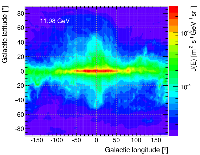
Figure 6: Map, in galactic coordinates, of the differential intensity of the LAT gll_iem_v05.fit model of the galactic diffuse emission in the energy slice centered at $\sim 12$ GeV.

Figure 7 shows the differential intensity for the $2^{\circ}\times 2^{\circ}$ square around the galactic center (the GDE spectrum in other part of our Galaxy, normalization aside, is fairly similar.)

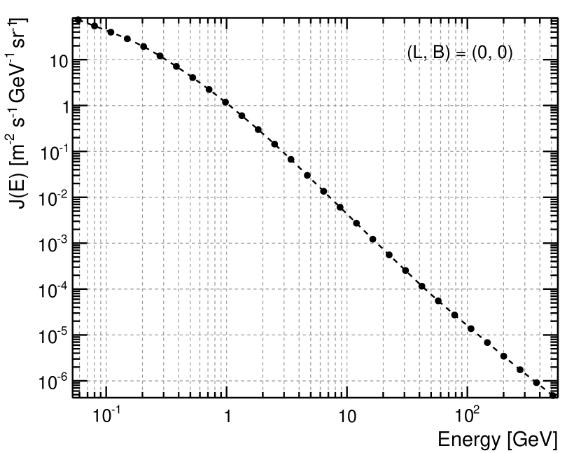
Figure 7: Differential intensity of the galactic diffuse emission around the galactic center for LAT gll_iem_v05.fit model. (Note that, this being a model—though tuned to the LAT data—it comes with no error bars.)

IV.4 Gamma-ray point sources

Based on two years of sky survey, the second Fermi-LAT source catalog (2FGL Nolan et al. (2012)) is the deepest ever gamma-ray catalog between 100 MeV and 100 GeV. It contains positional, variability and spectral information for 1873 sources detected by the LAT in this energy range.

We refer the reader to the fellow LAT second pulsar catalog Abdo et al. (2013), the second catalog of active galactic nuclei Ackermann et al. (2011) and first catalog of sources above 10 GeV Ackermann et al. (2013a) for more information about specific source populations.

IV.5 Gamma-ray isotropic background

What remains after the galactic diffuse emission and the point and extended sources have been subtracted from the gamma-ray all-sky intensity is generally referred to as isotropic gamma-ray background, or IGRB Abdo et al. (2010a). The IGRB is an observation-dependent quantity, as its intensity depends on how many sources are resolved in a give survey—and populations of faint sources below the detection threshold are guaranteed to contribute to it. The sum of the IGRB and the extra-galactic sources is, in some sense, a more fundamental quantity which is generally referred to as extra-galactic background (EGB).

From the experimental point of view, the measurement of the IGRB is challenging in that one has to discriminate an isotropic flux of gamma rays against the much brighter charged-particle foreground without any spatial or temporal signature to be exploited. We shall briefly come back to this in section IX.1.

IV.6 State of the art: modeling and measurements

Beautiful as they are, figures 3, 4, 5, 6 and 7 provide some of the most striking evidence for the tremendous body of knowledge about cosmic and gamma rays accumulated over the last century. On the theoretical side the progress has been no less spectacular, and we refer the reader to Blasi (2013) for an impressive, up-to-date and comprehensive review of the basic theoretical ideas at the basis of the so-called supernova paradigm for the origin of galactic cosmic rays.

In fact the discussion in the previous sections might very well give the reader the warm and fuzzy feeling that there is little left to discover, while nothing is farthest from truth. The aforementioned review Blasi (2013) makes a honest effort at highlighting the most important loose ends in our understanding of cosmic-ray production and propagation, and Ackermann et al. (2012b) provides a good summary of the difficulties involved in a self-consistent modeling of the galactic diffuse gamma-ray emission and the propagation of cosmic rays.

More importantly, at least from the prospective of this review, there are substantial pieces of observational evidence that are, to date, either missing or controversial. The feature in cosmic ray electron spectrum reported by the ATIC and BETS experiments in 2008, while not confirmed, at the time of writing, by at least three experiments (Fermi, PaMeLa and H.E.S.S) is a good example of an unexpected finding that has stirred the interest of the community triggering literally hundreds of follow-up papers (see figure 8).

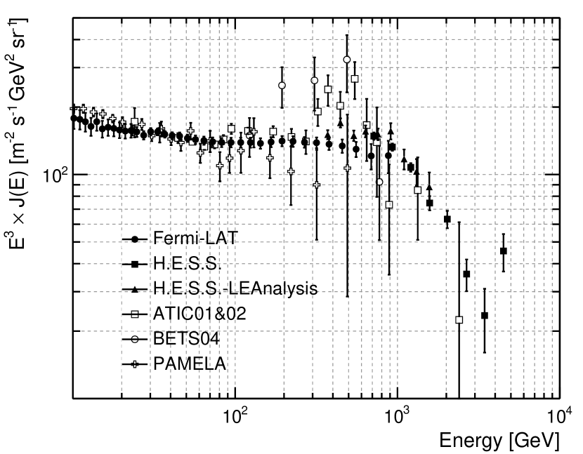
Figure 8: Compilation of some of the most recent measurements of the high-energy cosmic-ray $e^{+}+e^{-}$ spectra. Data points are from Ackermann et al. (2010); Aharonian et al. (2008, 2009); Chang et al. (2008); Yoshida et al. (2008); Adriani et al. (2011b).

More recently, the PaMeLa experiment has reported Adriani et al. (2011a) an abrupt change of slope around $\sim 230$ GV in the proton and helium spectra, whose extrapolation seem to nicely match the measurements at higher energies by CREAM Yoon et al. (2011) and ATIC Panov et al. (2009). This tantalizing piece of evidence, if confirmed, would be of tremendous interest, and is one of the notable examples of direct measurements where the community is holding its breath for the results from the AMS-02 experiment operating on the space station.

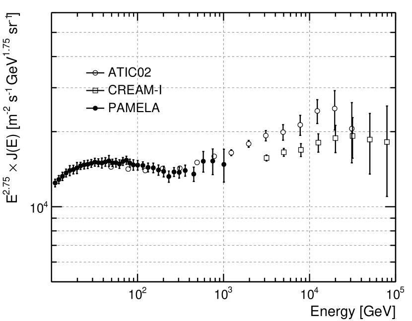
Figure 9: Compilation of the measurements of the high-energy proton spectrum by the PaMeLa Adriani et al. (2011a), CREAM Yoon et al. (2011) and ATIC Panov et al. (2009) experiments.

V Historical overview

As we mentioned in the previous section, the discovery of cosmic rays is customarily credited to Victor Hess for his balloon flights in the summer of 1912 Hess (1912). In fact, around the same time, several different scientists were carrying out investigations on the penetrating radiation with Wulf electroscopes, including Pacini Pacini (1912), Gockel and Wulf himself. By 1915 such instruments had been flown on balloons up to more than 8000 m, measuring a level of radiation much larger than that recorded by Hess in his first flight. The evidence for the extraterrestrial origin of the radiation was compelling.

Figure 10: Original measurements from one of the ascents performed by Viktor Hess (adapted from Hess (1912)). The rate of discharge increasing with altitude implies that the ionizing radiation responsible for it is coming from the outer space. (On an un-related note, no plot is included in the original article, which is by no means less beautiful.)

V.1 The early days

A vibrant and enlightening (though not necessarily unbiased) account of the first 50 years of research on cosmic rays is given by Bruno Rossi Rossi (1964). Interestingly enough, the question of the nature of the cosmic radiation did not get much attention until the end of the 1920s. The most striking known feature of cosmic rays was their high penetrating power and, for the first 15 years after their discovery, scientists implicitly assumed that they were gamma rays—the most penetrating radiation known at the time. This points to one of the most prominent difficulties that had to be faced in the early studies of the cosmic radiation: the fact that little or nothing was known about the physical interaction processes experienced by high-energy photons and charged particles. The first satisfactory theory of electromagnetic showers (see section VII.4), due to Bethe and Heitler, was published in 1934 Bethe and Heitler (1934); before that, people could only assume that high-energy gamma rays only interacted with matter via Compton scattering, whose cross section has been shown to decrease with energy by Dirac Dirac (1926) and Klein and Nishina Klein and Nishina (1929).

Robert Millikan formulated the first complete theory of comic rays, based on all the measurements of attenuation in the atmosphere and in water available at the time Millikan and Cameron (1928). He proposed that the primary cosmic radiation was composed of gamma rays of well-defined energies, produced in the interstellar space by the the fusion of hydrogen atoms in heavier elements—and that the charged particles observed in the Earth atmosphere were electrons produced via Compton scattering. Though we know, a posteriori, that this idea did not pass the test of time, the original papers are still an interesting reading.

The begin of the post-electroscope era, around 1929, largely relies on a few fundamental technical breakthroughs: the development of the Geiger-Müller tubes, the first practical implementations of the coincidence technique, introduced by Bothe and Kolhörster Bothe and Kolhörster (1929) and refined by Bruno Rossi Rossi (1930a), and the introduction of imaging devices such as the bubble chamber (and, later, the cloud chambers and the stacks of photographic emulsions sensitive to single charged particles).

It was thanks to different clever arrangements of Geiger tubes in coincidence and shielding materials that an incredible amount of new information about cosmic rays was made available in the 1930s. It soon became clear that some of the particles observed could pass through very noticeable amounts of material, which casted serious doubts on the interpretation of the primary component as consisting of photons.

At about the same time, physicists realized that the interaction between radiation and matter was much more complicated that they had anticipated. In 1933 Blackett and Occhialini Blackett and Occhialini (1933) published the results of the first observations performed with a cloud chamber triggered by Geiger-Müller tubes, clearly showing the copious production of secondary radiation and the new phenomenon of the showers. This, in turn, forced scientists to focus the attention on the genetic relation between the primary and the secondary components of the cosmic radiation, and to consider seriously the hypothesis that most of the particles observed near the surface were actually produced in the atmosphere.

The idea that the magnetic field of the Earth could be used to shed light on the nature of the cosmic radiation, and establish unambiguously whether primary cosmic rays were photons or charged particles occurred early on in the 1920s. It was clear that, in the second case, they would be somewhat channeled along the field lines and one would expect a larger intensity at the magnetic poles compared to the equator. Searches for this latitude effect were carried out as soon as 1927, but it is fair to say that in 1930, when Bruno Rossi started the first quantitative analysis of the problem, evidence for an influence of the geomagnetic field on the intensity of the cosmic radiation were far from being compelling (the latitude effect was only established in the 1930s thanks to a monumental measurement campaign led by A. H. Compton). Building on top of the work by the Norwegian geophysicist Carl Störmer, Rossi set the stage for the ray-tracing techniques which are nowadays customarily used to study the motion of charged particles in a magnetic field (see section VI.2.3). He predicted that, if the primary cosmic rays were charged, and predominantly of one sign (either positive or negative), one should observe an East-West flux asymmetry, which would be maximal around the geomagnetic equator (see section VI.2.5). In 1934 Rossi Rossi (1930b) and two other groups independently measured this East-West effect. It was an incontrovertible evidence that primary cosmic rays are charged—and, even more, the sign of the effect allowed to predict the prevalent sign of their charge. “The results of these experiments […] confirm the view, supported by the early experiments of the writer, that cosmic rays consist chiefly of a charged corpuscular radiation with a continuous energy spectrum extending to very great energies. Moreover the new results on the azimuthal effect show that the charge is predominantly positive. It is however possible that, in addition to the positive particles, a smaller amount of other kind of rays (negative particles, photons, neutrons) is contained in the cosmic radiation. In fact, some results are rather difficult to explain by supposing that the cosmic radiation consists merely of positive particles.” These brief except from Rossi (1930b), written in 1934, still constitutes a substantially correct description of our current understanding of cosmic rays.

On a slightly different note, we should emphasize that we deliberately left out from this short summary at least two fundamental items. The first is the deep connection between cosmic rays and the early stages of development of particle physics, with the positron Anderson (1933), muon Neddermeyer and Anderson (1937); Street and Stevenson (1937) and pion Lattes et al. (1947) all being discovered in the cosmic radiation. The other is the discovery of extensive air showers Auger et al. (1939), which originated an independent (and incredibly prolific) line of research—that of the study of ultra-high-energy cosmic rays from the ground.

All this said, it is fair to say that between 1940 and 1950 a complete and coherent picture of the phenomena connected with the cosmic radiation emerged, with most of the primary cosmic rays being protons and nuclei of heavier elements and most of the particles observed near to the surface being secondary products of their interaction with the atmosphere. As we shall see in a second, the development of stratospheric balloons and the beginning of the space age allowed to customarily observe the primary radiation at the top of the atmosphere in the following decades.

V.2 The latter days

The launch of the Sputnik I artificial satellite by the Soviet Union on October 4, 1975 signals the begin of the space era. Within six months the Sputnik II soviet satellite and the Explorer I and Explorer III American satellites were launched—all the three of them were equipped with Geiger-Müller counters with the aim of mapping the comic-ray intensity beyond the altitudes reachable by balloons (the Explorer I and Explorer III were placed into an elliptical orbit reaching out to some 2500 km). One of the most interesting discoveries was that of the Van Allen belts van Allen (1959)—regions around the Earth where low-energy charged particles trapped in the geomagnetic field make the cosmic-ray intensity several orders of magnitude more intense than that on the surface.

As it turns out, the radiation belts are not directly relevant for instruments in low-Earth orbit (which is the main topic of this write-up), with the notable exception of the South Atlantic Anomaly that we shall briefly introduce in section VI.2.7. We shall glance through the basics of geomagnetically trapped radiation (which, in general, is relevant for the low-Earth orbit environment) in section VI.2.6.

V.2.1 Charged cosmic rays

It is fair to say that, among the first modern instruments for charged cosmic-ray measurements are the pioneering magnetic spectrometers flown on balloons in the 1960s and 1970s for the study of the positron Fanselow et al. (1969); Daugherty et al. (1975); Buffington et al. (1974) and the antiproton Bogomolov et al. (1979); Golden et al. (1984a) components of the cosmic radiation. They generally had limited (at least by any modern standard) energy range and particle identification capabilities—typically provided by a Cherenkov detector.

On a related note, it is somewhat amusing to note how back in the 1980s the apparent increase of the positron fraction above $\sim 5$ GeV that these early measurements seemed to indicate was actively discussed, and both pulsars and dark matter annihilation were already proposed as viable candidates for its origin Boulares (1989). And then the history repeated itself two decades later (this time for real) with the measurement published by the PaMeLa collaboration Adriani et al. (2009a).

At about the same time emulsion chambers Kobayashi et al. (2012); Cherry (2006) and calorimetric experiments Meegan and Earl (1975); Hartmann et al. (1977); Tang (1984) were used for the measurement of the all-electron and the proton and nuclei spectra.

WiZard Golden et al. (1990) was the name of the magnetic spectrometer concept selected in the late 1980s for the Astromag facility planned to operate on the U.S. Space Station Freedom—which never saw the light as originally conceived and later evolved into the International Space Station. As this project was abandoned, the WIZARD collaboration Spillantini (2003) started a long and incredibly successful campaign of balloon-borne experiments—including MASS89, MASS91, TS93, Caprice94, Caprice97 and Caprice98—which finally winded up in the PaMeLa space-based magnetic spectrometer, currently in operation. HEAT and BESS (see section V.3.3) constitute two additional notable examples of magnetic spectrometers flown around the same time. Generally speaking, the 1990s signal a dramatic leap forward in the particle identification capabilities of the instruments, with transition radiation detectors and advanced Cherenkov detectors effectively exploited, and modern imaging calorimeters providing shower-topology information in addition to the basic energy measurement.

At this point we are straight into the present, with the AMS-02 magnetic spectrometer operating on the International Space Station—preceded by the Shuttle flight of the path-finder AMS-01 in 1998—and, on the calorimetric side of the panorama, the fabulous four balloon-borne detectors: ATIC, CREAM, TIGER and TRACER. One a related note, the record-breaking 161 days of exposure integrated by CREAM in its six flights signal the exciting perspectives nowadays made available by the development for Long Duration (LD) circumpolar balloon flights.

V.2.2 Gamma rays

The Explorer XI satellite, launched in 1961, carried a gamma-ray detector on board, consisting of a crystal scintillator and a Cherenkov counter, surrounded by an anti-coincidence shield Kraushaar and Clark (1962a). While the satellite could not be actively pointed and the photon direction was loosely determined by the solid angle defined by the geometry of the telescope, Explorer XI performed the first observation of the gamma-ray sky and in 1962 the beginning of gamma-ray astronomy was announced to the world on Scientific American: “An ingenious telescope in a satellite has provided the first view of the Universe at the shortest wavelength of the electromagnetic spectrum. This historic glimpse is supplied by just 22 gamma rays.” Kraushaar and Clark (1962b).

Experiment	Energy range	Date	$\gamma$ candidates
Explorer XI	$>50$ MeV	1961	22
OSO-3	$>50$ MeV	1967–1968	621
SAS-2	20 MeV–1 GeV	1972–1973	13,000
COS-B	30 MeV–3 GeV	1975–1983	200,000
EGRET	30 MeV–10 GeV	1991–1999	1,500,000
Fermi-LAT	20 MeV–$>1$ TeV	2008–??	500,000,000

Table 3: Total number of gamma-ray candidates collected by specific space-born detectors through their missions. Note that the energy ranges for the various experiments are purely indicative.

A similar detector concept was flown in 1967 on board the third Orbiting Space Observatory (OSO-3). OSO-3 operated continuously for 16 months (at which point the last spacecraft tape recorder failed), performing a complete sky survey and recording 621 photons above 50 MeV. Most notably, the experiment demonstrated that celestial gamma-rays are anisotropically distributed—concentrated in the direction of the galactic plane and, particularly, toward the galactic center.

In 1969 and 1970 the array of military satellites VELA, launched by the United States to monitor possible nuclear experiments carried out by the Soviet Union, serendipitously discovered the transient flashes of gamma radiation that generally go under the name of gamma-ray bursts (GRB).

It is generally acknowledged that SAS-II Derdeyn et al. (1972), launched on November 1972, provided the first detailed information about the gamma ray sky and effectively demonstrated the ultimate promise of gamma-ray astronomy, showing that the galactic plane radiation was strongly correlated with the galactic structural features—not event mentioning the first detection of gamma-ray point sources, most notably the Vela and Crab pulsars. SAS-II was the first satellite entirely devoted to gamma-ray astrophysics, with a gamma-ray telescope on board composed by spark chambers interleaved with tungsten conversion foils , and an anti-coincidence system featuring a set of plastic scintillator tiles and directional Cherenkov detectors placed below the spark chambers. With a peak effective area of $\sim 120$ cm² and a PSF of the order of a few degrees, the gamma-ray detector on board SAS-II is effectively one of the first incarnations of the pair conversion telescope concept (see section V.3.2).

In 1975 the European Space Agency launched the COS-B Bignami et al. (1975) satellite, that operated successfully for 6 years and 8 months—well beyond the original goal of two years. The gamma-ray telescope on board COS-B was conceived following the heritage of that on SAS-II, with the crucial addition of a $4.7~{}X_{0}$ calorimeter to improve the energy measurement. It was sensitive to photons between 30 MeV and several GeV over a field of view of almost 2 sr, with a peak effective area of some 50 cm². Among the key science results from the COS-B mission are the first catalog of gamma-ray sources (including 25 entries) and a complete map of the disc of the milky way.

With a weight of approximately 17 tons, the Compton Gamma Ray Observatory (CGRO), launched by NASA in 1991, is possibly the heaviest scientific payload ever flown in low-Earth orbit. The Energetic Gamma Ray Experiment Telescope (EGRET Kanbach et al. (1988)) on board CGRO, a pair conversion telescope with far superior sensitivity than any of its predecessors, made the first complete survey of the gamma-ray sky in the energy range between 30 MeV and $\sim 10$ GeV (detecting 271 discrete sources) and is at the base of the last-generation instruments exploiting the silicon-strip technology such as AGILE and the Fermi-LAT Atwood et al. (2009).

Figure 11: Total number of gamma-ray candidates collected by specific space-born detectors through their missions. The points on the $x$-axis are the average values between the mission start and stop times.

Table 3 summarizes the number of gamma-ray candidates collected by the gamma-ray detectors listed in this section through the duration of the corresponding mission. While the numbers surely give a sense of the continuous advance in performance, there are good reasons (primarily geometrical dimensions and weight) to presume that it is going to be hard to keep up with this sort of Moore’s law (see figure 11) over the next few years.

V.3 Instrument concepts

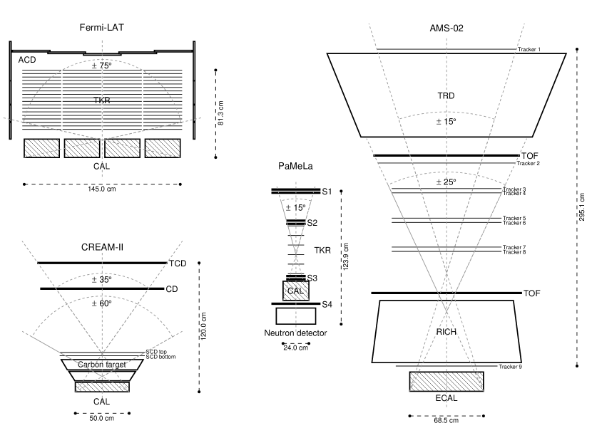
Figure 12: Schematic view of some of the most recent space- or balloon-borne cosmic-ray and gamma-ray detectors (all the dimensions are meant to be in scale). Only the detector subsystems are sketched (note that the magnets for PaMeLa and AMS-02 are not represented). For the Fermi-LAT: the anti-coincidence detector (ACD), the tracker (TKR) and the calorimeter (CAL). For AMS-02: the transition radiation detector (TRD), the time of flight (TOF), the tracker layers, the electromagnetic calorimeter (ECAL) and the ring imaging Cherenkov detector (RICH). For CREAM-II: the timing charge detector (TCD), the Cherenkov detector (CD), the silicon charge detector (SCD) and the calorimeter (CAL). For PaMeLa: the time of flight scintillators (S1–S3), the tracker (TKR), the calorimeter (CAL) and the neutron detector. For each instrument the relevant combination of sub-detectors determining whether a given event is reconstructable (and hence the field of view) is also sketched. Trivial as it is, we also note that the calorimeters are made of different material and therefore the relative thickness does not necessarily reflect the depth in terms of radiation lengths (this information is included in table 4).

Experiment	Peak $G$ [m2 sr]			$T_{\rm obs}$ [year]	$\sigma E/E$		References
	$e^{\pm}$	$\gamma$	$p$/nuclei		$e^{\pm}$, $\gamma$	$p$/nuclei
Agile	–	0.1	–	$>7$	$\sim 100\%$ 400 MeV	–	Tavani et al. (2009)
AMS-02	0.05			20	2% @ 50 GeV	–	Brient et al. (2013); Ting (2013)
ATIC	0.24			0.15	2% 150 GeV	35%	Ganel et al. (2005)
CREAM	–	–	0.43	0.5	6% 200 GeV	40%	Yoon et al. (2011)
Fermi	2.8 @ 50 GeV	2.0 @ 10 GeV	–	10	5–15%	–	Ackermann et al. (2012c); Ackermann et al. (2010)
PaMeLa	0.00215	–	0.00215	7	5–10%	–	Picozza et al. (2007)
TRACER	–	–	4.73	0.05	–	See Obermeier et al. (2011)	Obermeier et al. (2011)
CALET	0.12			5	2% @ 1 TeV	40% @ 1 TeV	Mori (2013)
DAMPE	0.3	0.2	0.2	3	1.5% @ 800 GeV	40% @ 800 GeV	–
Gamma-400	0.5			7	1% @ 10 GeV	–	Galper et al. (2013)
Gamma-400 (CC)	3.4 @ 1 TeV		3.9 @ 1 TeV	7	2% @ 1 TeV	35% @ 1 TeV	–
HERD	$>3$		$>2$	10	1% @ 100 GeV	20% @ 1 TeV	Zhang and the HERD collaboration (2014)

Table 4: Summary table with the main characteristics of some of the cosmic-ray and gamma-ray instruments that have started operation after the year 2000. Note that, despite the effort that has been put in extracting the numbers from the available literature, it is likely that some of them will be slightly incorrect. Although the topic is is not discussed (yet) in this write-up, the bottom part of the table does include some of the most prominent instrument that are now in the design or implementation phase (the reader is advised that that corresponding figures are subject to change without notice).

The brief summary of the history of cosmic-ray measurements we have outlined in the previous two sections is also an illustration of the basic detector concepts and experimental techniques that have been exploited over the last $\sim 50$ year. The dichotomy between magnetic spectrometers and calorimetric experiments is a fundamental one and we shall elaborate a little bit more on it in the next section. We postpone a (much) more in-depth discussion of some related technical aspects to sections VIII and IX. Schematic views of a few actual instruments, either recent or in operation, are shown (in scale!) in figure 12.

V.3.1 Spectrometers and calorimeters

Most modern comic-ray detectors fall in either of the two categories: magnetic spectrometers or calorimetric experiments. Strictly speaking all the advanced magnetic spectrometers feature an electromagnetic calorimeter for energy measurement, so the basic difference between the two is really the presence of the magnet.

The key feature of magnetic spectrometers is their ability of distinguishing the charge sign—e.g., separating electrons and positrons or protons and antiprotons. In addition, they are typically equipped with additional sub-detectors (Cherenkov detectors and/or transition radiation detectors) aimed at particle identification, e.g., for isotopical composition studies (see section VIII.5.2). This all comes at a cost, in that the magnet is a passive element (and typically a heavy one) contributing to the mass budget and limiting the field of view (not even mentioning the potential issue of the background of secondary particles). Both effect conspire to make the acceptance of this kind of instrument relatively smaller.

Calorimetric experiments, on the other hand, typically feature a larger acceptance and energy reach—and are best suited for measuring, e.g., the inclusive $e^{+}+e^{-}$ spectrum or the proton and nuclei spectra up to the highest energies—but cannot readily separate charges (see, however, section VI.2.8 for yet another twist to the story). Modern electromagnetic imaging calorimeters, be they homogeneous or sampling, provide excellent electron/hadron discrimination and are typically instrumented with some kind of external active layer for the measurement of the absolute value of the charge (e.g., to distinguish between singly-charged particles and heavier nuclei). Since flying an accelerator-type hadronic calorimeter in space is impractical due to mass constraints (see section VIII.4.2), a fashionable alternative to measure the energy for hadrons is that of exploiting a passive low-Z target (as done, e.g., in the CREAM and ATIC detectors) to promote a nuclear interaction and then recover the energy from the electromagnetic component of the shower.

V.3.2 Pair-conversion telescopes

In the basic scheme laid out in the previous section gamma-ray pair conversion telescopes are essentially calorimetric experiments featuring a dedicated tracker-converter stage in which foils of high-$Z$ materials are interleaved with position sensitive detection planes. The basic detection principle is easy: the conversion foils serve the purpose to promote the conversion of high-energy (say above $\sim 20$ MeV) gamma rays into an electron-positron pair which is in turn tracked to recover the original photon direction. The pair is then absorbed into the calorimeter for the measurement of the gamma-ray energy. Last but not least, pair conversion telescopes feature some kind of anti-coincidence detector for the rejection of the charged-particle background that, as we have seen, outnumbers the signal by several orders of magnitude in typical low-Earth orbit.

As mentioned in section V.2.2, EGRET Kanbach et al. (1988) on-board the CGRO mission, AGILE and the Fermi-LAT Atwood et al. (2009) are prototypical examples of pair-conversion telescopes.

V.3.3 Unconventional (or just old-fashioned) implementations

While most of the detectors we shall consider in the following are built around either a magnetic spectrometer a la AMS-02 or an electromagnetic calorimeter, there exist less conventional implementations that deserve to be briefly mentioned, here.

Among the magnetic spectrometers, BESS (see, e.g., Yamamoto et al. (2002)) is a notable example where the instruments features a thin superconducting solenoid magnet enabling a large geometrical acceptance with a horizontally cylindrical configuration (note that in this case the particles go through the magnet!). Several different versions of the instrument underwent a long and very successful campaign of balloon flight for the measurement (and monitoring in time) of the antiproton BESS Collaboration et al. (2008) and proton and helium spectra Sanuki et al. (2000).

With its unrivaled imaging granularity, the emulsion chamber technique played a prominent role in the early days of calorimetric experiments, as it readily allowed to assemble large—and yet relatively simple—detectors. In this case it is the data analysis process that is significantly more difficult to scale up with the available statistics with respect to that of modern digital detectors. Reference Kobayashi et al. (2012), e.g, contains a somewhat detailed summary of more than 30 years of observations of high-energy cosmic-ray electrons—in several balloon flights from 1968 to 2001—with a detector setup consisting of a stack of nuclear emulsion plates, X-ray films, and lead/tungsten plates. Electromagnetic showers were detected by a naked-eye scan of the X-ray films and energies were determined by counting the number of shower tracks in each emulsion plate within a 100 $\mu$m wide cone around the shower axis. At even higher energies, a nice account of the emulsion chambers (e.g., JACEE Burnett et al. (1986) and RUNJOB Derbina et al. (2005)) flown on balloons with the aim of measuring the cosmic-ray chemical composition near the knee is given in Cherry (2006).

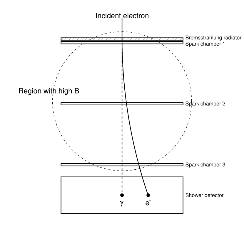
Figure 13: Schematic diagram of a magnetic spectrometer equipped for the bremsstrahlung-identification technique (adapted from Buffington et al. (1974)).

We close this section by mentioning the bremsstrahlung-identification technique, used, e.g., in  Buffington et al. (1974), which strikes the author as one of the neatest and most clever attempts to overcome the limited particle identification capabilities of the early detectors. The basic idea, illustrated in figure 13, is that of using a thin radiator and select the electrons and positrons producing a bremsstrahlung photon—identified as an additional individual shower in the calorimeter (or really, in the shower detector). Though the overall fraction of useful signal events is somewhat reduced, this detector concept provides a clear and distinct signature (that is very hard to mimic for heavy particles) allowing proton rejection factors of the order of $10^{5}$.

V.3.4 Different instrument concepts

All the cosmic-ray detectors we have mentioned so far exploit nuclear interactions to measure the energy of protons and heavier nuclei. In contrast to calorimetric measurements, it is possible, at least in principle, to measure the cosmic-ray charge and energy through their electromagnetic interaction only. The main advantage is that this concept makes it possible to realize instruments with very large geometrical aperture (of the order of several m² sr before selection cuts), as only low-density material are necessary. On the other hand, the main drawback is that the quality of the energy measurement is largely non uniform across the energy range covered—and poor-to-non existent in some significant portions of the phase space.

The TRACER balloon-borne detector Obermeier et al. (2011) is possibly the most notable example of this type of instrument concept. By a clever combination of scintillators, Cherenkov detectors, transition radiation detectors and a $dE/dx$ array (see sections VII and VIII for more details), TRACER was able to measure the charge and the energy of cosmic-ray nuclei with $Z>5$ between $\sim 1$ GeV and a few TeV. Figure 14 shows the response functions, normalized by $Z^{2}$, for the three basic TRACER sub-detectors: the charge is measured by the $dE/dx$ array—with the Cherenkov detectors breaking the degeneracy between the two parts of the curve on the two sides of the minimum—while the energy is recovered from the Cherenkov detectors near the Cherenkov threshold, from the $dE/dx$ array in the intermediate range (admittedly with limited resolution), and from the TRD at very high energy.

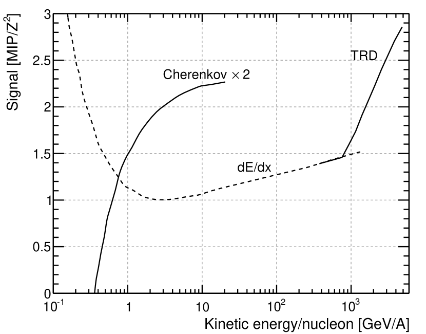
Figure 14: Response functions, normalized by $Z^{2}$ for the three basic TRACER sub-detectors (adapted from Obermeier et al. (2011)). Much more details about the basic physical interaction processes and how these can be exploited in actual particle detectors can be found in sections VII and VIII.

On a completely different subject, we briefly mention the Compton telescope concept, which constitutes one of the possible experimental approaches for studying gamma rays below $\sim 20$ MeV—where Compton scattering is the interaction physical process with largest cross section. The basic idea is that of measuring both the (first) Compton interaction point through the scattered electron and the direction of the scattered photon by absorbing it. This, in turn, allows to kinematically constraint the direction in the sky of the original gamma-ray in the so called Compton cone. As it turns out, any practical implementation of this seemingly simple concept is quite challenging, for many different reasons. It is not by coincidence that the last Compton telescope flow in space was COMPTEL Schoenfelder et al. (1993) on-board the CGRO, totaling $\sim 50$ cm² on-axis effective area—a somewhat meager figure when considering that the total weight of the instrument was of the order of 1 ton.

VI The near-Earth environment

This section deals with the basic characteristics of the environment in which balloon and/or satellites in low-Earth orbit operate. There are two main aspects of the problem, namely the atmosphere and the geomagnetic field.

VI.1 The atmosphere of the Earth

The simplest possible model for the Earth’s atmosphere is that of an isothermal gas in hydrostatic equilibrium. Under the assumption that the magnitude of the gravitational field of the Earth does not change significantly with the altitude $h$, the problem can be analytically integrated and the result is that the pressure follows a simple barometric profile

$$p(h)=p_{0}\exp\left(-\frac{h}{h_{0}}\right),$$ (13)

with a pressure at sea level $p_{0}\sim 101.325$ kPa. It goes without saying that, in this naïve model, the density follows the very same scale law:

$$\varrho(h)=\varrho_{0}\exp\left(-\frac{h}{h_{0}}\right),$$ (14)

with a density at sea level of $\varrho_{0}\sim 1.24\times 10^{-3}$ g cm^-3. One can actually show that the isothermal scale height at a given temperature $T$ is related to the basic physical properties of the atmosphere by the simple relation

$$h_{0}=\frac{RT}{g\mu},$$ (15)

where $R$ is the ideal gas constant, $g$ is the gravitational acceleration and $\mu$ is the average molecular mass. By plugging the numbers into equation (15), one obtains a scale height of $h_{0}\sim 7.9$ km at $270^{\circ}$K (dry air contains about 78% of N₂, 21% of O₂ and small amounts of other gases, for an average molecular mass $\mu\sim 29$).

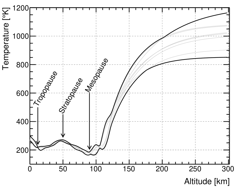
Figure 15: Illustrative atmospheric temperature profiles provided by the NRLMSISE-00 model Picone et al. (2002). The thin gray lines represent the model values for 8 reference points on the Earth’s surface (4 on the equator and 4 at $60^{\circ}$ latitude), while the black thick lines represent the envelope of such models. Data are taken from %****␣sec_environment.tex␣Line␣50␣****http://ccmc.gsfc.nasa.gov/modelweb/models/nrlmsise00.php.

Unfortunately life is not that easy, as the temperature profile of the Earth atmosphere is a complicated function of the altitude, with its different regimes defining the standard atmospheric layers: the troposphere ($0$–$12$ km), the stratosphere ($12$–$50$ km), the mesosphere ($50$–$90$ km) and at even larger altitudes, the thermosphere and the exosphere. Figure 15 shows some illustrative temperature profiles, as given by the NRLMSISE-00 Picone et al. (2002) empirical atmospheric model, for different locations on the surface of the Earth. One of the most striking features of such profiles is the temperature increase above $\sim 100$ km, which is essentially due to the absorption of ultraviolet radiation from the Sun. Before the reader starts wondering whether a satellite in low-Earth orbit (i.e. orbiting at a few hundred km above the Earth’s surface) is really immersed in a thermal bath at $\sim 1000^{\circ}$K, it is worth stressing that this figure is merely a measure of the average molecular kinetic energy. As a matter of fact, as we shall see in a moment, at these altitudes the average density is so small that convection play essentially no role as a heat exchange mechanism. Discussing in details all the physical processes playing a role in the physics of the atmosphere is obviously beyond the scope of this review.

That all said, we note that for altitudes smaller than $\sim 100$ km the temperature is, roughly speaking, approximately constant, so that our simple-minded isothermal model (14) can be expected to work reasonably well. This is illustrated in figure 16, where the density profiles from the same empirical model used in figure 15 are compared with an isothermal model with scale height $h_{0}=7$ km.

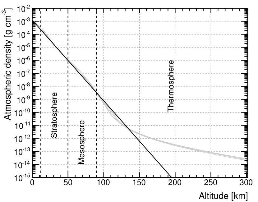
Figure 16: Illustrative atmospheric density profiles provided by the NRLMSISE-00 model. The thin gray lines represent the model values for 8 reference points used for figure 15, while the black line is the prediction of an isothermal model (14) with scale height $h_{0}=7$ km.

VI.1.1 Typical balloon floating altitude

The basic figures in the previous section can be used for a rough calculation of the typical balloon floating altitude. We shall assume a volume $V_{b}$ at full expansion of $10^{6}$ m³, filled with He gas, and a mass of the payload $m_{p}$ of 3 tons. At the same pressure and temperature the ratio between the densities of He and air is approximately equal to ratio of the atomic weights:

$$r_{\varrho}=\frac{\varrho_{\rm He}}{\varrho_{\rm Air}}\sim\frac{4}{29}\sim 0.14.$$

The floating altitude is determined by Archimedes’ principle—essentially we have to equate the buoyant force to the weight of the payload:

$$(1-r_{\varrho})V_{b}\varrho_{0}\exp\left(-\frac{h_{\rm float}}{h_{0}}\right)=m_{p},$$

which is readily solved for $h_{\rm float}$:

$$h_{\rm float}=-h_{0}\ln\left[\frac{m_{p}}{(1-r_{\varrho})V_{b}\varrho_{0}}\right].$$ (16)

By plugging in the actual numbers one gets a value of $h_{\rm float}\sim 41$ km, which is only slightly in excess of the typical floating altitude of actual scientific balloons.

VI.1.2 The atmospheric grammage

A relevant physical quantity related to the atmospheric density is the integrated column density above a given altitude, sometimes called the atmospheric overburden

$$\chi(h)=\int_{h}^{\infty}\varrho(h^{\prime})\;dh^{\prime}.$$ (17)

If we limit ourselves to the stratosphere, the part of the integral above $\sim 100$ km can be effectively neglected and we can use our isothermal model (14), which is readily integrated:

$$\chi(h)=\varrho_{0}h_{0}\exp\left(-\frac{h}{h_{0}}\right).$$ (18)

(The result of the integration is shown in figure 17.)

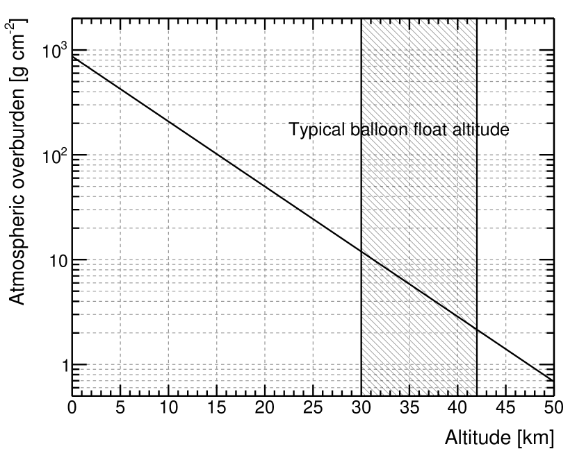
Figure 17: Atmospheric overburden as a function of the altitude calculated by integrating our baseline isothermal model. The shaded region indicates the typical float altitude of stratospheric balloons, where the effective overburden is of the order of a few g cm^-2.

First of all, the atmospheric overburden at sea level is $\varrho_{0}h_{0}\sim 900$ g cm^-2. In physical terms this means that the integrated density profile is equivalent to a $7$ km long column with constant density $\varrho=1.24\times 10^{-3}$ g cm^-3. Just to put things in context, this translates into $\sim 80$ cm, when re-scaled to the density of lead ($11.35$ g cm^-3). In other words, when viewed as a gigantic calorimeter, the Earth’s atmosphere is effectively equivalent to $\sim 80$ cm of lead. This is the basic reason why primaries above $\sim 10$ eV do not reach the Earth’s surface.

For reference, the atmospheric overburden at $40$ km above the sea level (which is the typical float height for balloons), is $\sim 3$–$4$ g cm^-2. This is an important number, as it is comparable with the propagation path length of cosmic rays in the Galaxy, which means that balloon-borne experiments have to correct the measured flux to recover the actual flux at the top of the atmosphere.

VI.1.3 The Earth Limb

So far we have convinced ourselves that the Earth’s atmosphere is important because it effectively prevents CR primaries from reaching the surface—and constitute some target material even for stratospheric balloon experiments. (Last but not least, as we know, the atmosphere makes the balloons float, which, although kind of obvious, it is indeed relevant for this review.)

There is yet another twist to the story that it’s worth mentioning—the fact that the Earth’s atmosphere, acting as a target for high-energy cosmic-ray protons and nuclei, effectively constitutes the strongest high-energy gamma-ray source in low-Earth orbit. The detailed modelization of the so called Earth limb emission requires a fair number of inputs, but the main characteristics can be understood on general grounds.

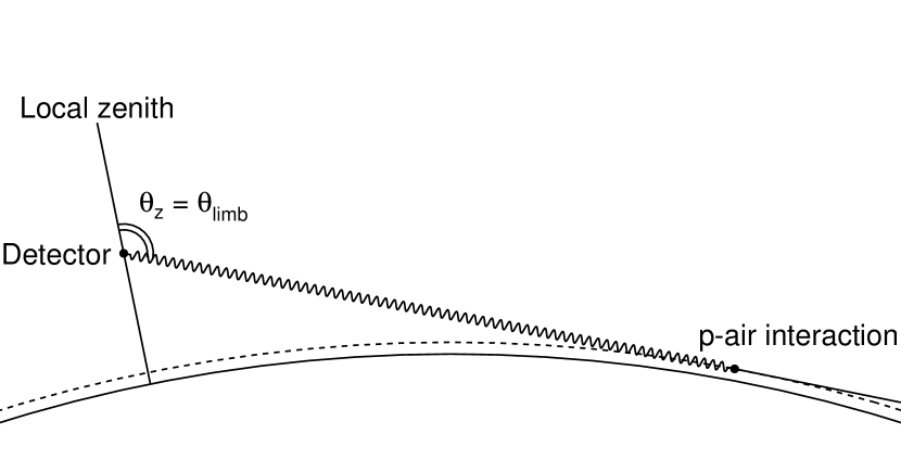
Figure 18: Sketch of the Earth limb gamma-ray emission mechanism: a primary cosmic-ray proton interacts at the top of the atmosphere (represented by the dashed line) and, among the final products, a photon (typically from the decay of a $\pi^{0}$) escapes the atmosphere in the forward direction.

The limb emission is mainly originating from cosmic-ray protons tangentially interacting near the top of the atmosphere and producing gamma rays in the forward direction, as sketched in figure 18 (this is especially true at high energy, where the secondaries are highly collimated due to momentum conservation). The viewing angle at a given detector altitude $h_{\rm det}$ reads

$$\theta_{\rm limb}=90^{\circ}+\arccos\left(\frac{R_{E}+h_{\rm atm}}{R_{E}+h_{\rm det}}\right),$$ (19)

where $h_{\rm atm}$ is the height of the top of atmosphere and $R_{E}$ the radius of the Earth. (We shall see in a moment that the top of the atmosphere, in this context, is really the maximum height at which a cosmic-ray protons impinging tangentially encounters enough material to have a non-negligible interaction probability.) For $h_{\rm atm}=50$ km and $h_{\rm det}=565$ km (the latter being representative of the height of the Fermi orbit), one gets $\theta_{\rm limb}\sim 112^{\circ}$. At smaller zenith angles cosmic rays do not interact while at larger angles the photons produced in the atmosphere are readily absorbed, so that the limb emission is (more or less narrowly, depending on the energy) peaked around $\theta_{\rm limb}$. As shown in figure 19, the gamma-ray emission from the limb of the Earth typically outshines the average gamma-ray all-sky intensity by 1 to 2 orders of magnitude (though it should be emphasized that it is only covering a relatively limited solid angle).

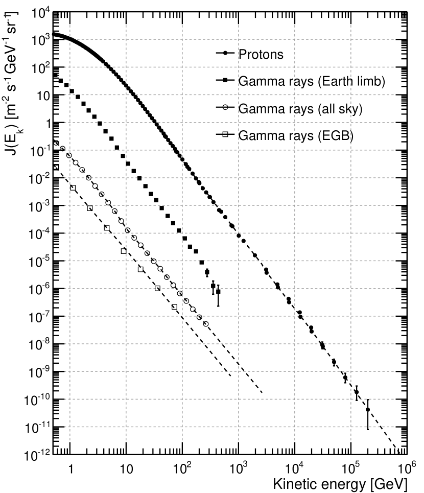
Figure 19: Intensity of the Earth limb measured by Fermi for the range of zenith angles $110^{\circ}<\theta_{z}<114^{\circ}$ (adapted from Abdo et al. (2009), notably with a different convention for how $\theta_{z}$ is measured). At the peak of its emission the limb outshines the average gamma-ray all-sky intensity by 1 to 2 orders of magnitude. It should also be noted that the high-energy spectral index follows that of primary protons, from which the limb emission originates.

We can actually move a little bit further in understanding the basics of the limb emission before things get too complicated. Following Abdo et al. (2009) we shall take the $p^{14}$N total inelastic cross section of $\sim 275$ mb as representative of the $p$-air cross section. Given the number density $n$ of targets per unit volume (expressed in nitrogen atoms per cm³), this figure can be converted in a proton mean free path through the well known relation

$$\lambda=\frac{1}{n\sigma}.$$ (20)

The number density and the actual density are related to each other by

$$\varrho=\frac{nA}{N_{A}},$$ (21)

where $A$ is the mass number of the target and $N_{A}$ the Avogadro number. We can therefore rewrite (20) as

$$\lambda\varrho=\frac{A}{N_{A}\sigma}$$ (22)

and, by plugging in the actual numbers ($A\sim 14$ and $\sigma\sim 275$ mb), we get a mean free path $\lambda_{p}\sim 85$ g cm^-2. The other relevant scale, here, is the radiation length of the air, which is $\sim 37$ g cm^-2 (see table 5). We can now define the concept of the “top of the atmosphere” introduced before somewhat more precisely: gamma-ray production takes place with a reasonable efficiency when the integrated column density is not negligible compared to mean inelastic free path $\lambda_{p}$, but is significantly attenuated when the column density is comparable or larger than the radiation length of the air—which leaves a relatively small angular window left, where the column density is of the order of a few times $\sim 10$ g cm^-2, for efficient production.

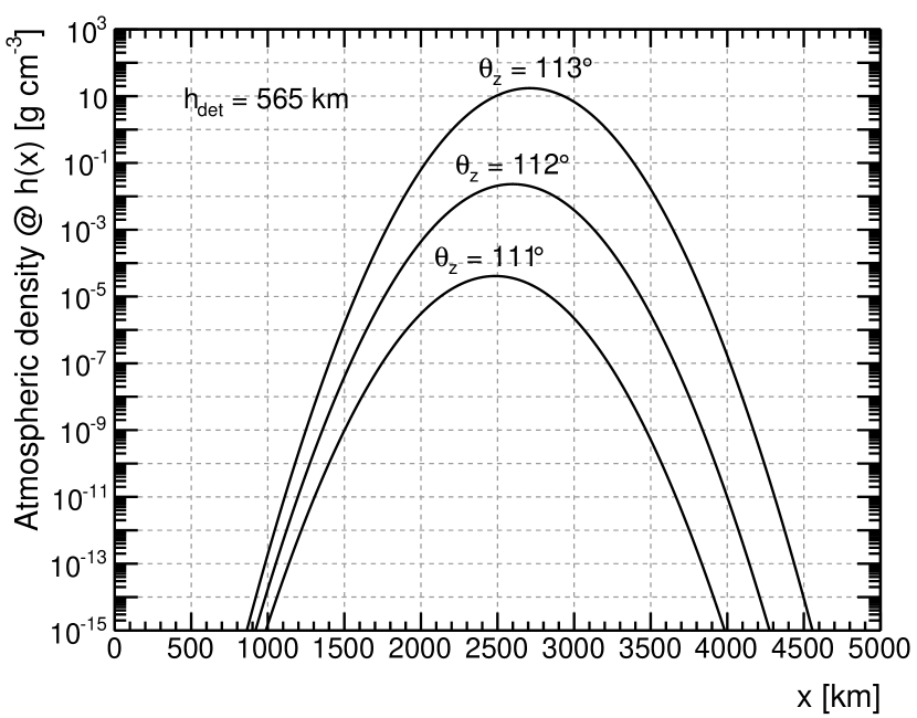
Figure 20: Profile of the atmospheric density traversed by a primary cosmic ray impinging on a detector at 565 km altitude for three (slightly) different zenith angles.

The integrated column density at a given zenith angle $\theta_{z}$ can be readily calculated given an atmospheric model. The altitude at a distance $x$ from the detector along the line of incidence of the primary cosmic ray can be written (by the Carnot theorem) as

$$h(x)=\sqrt{R_{\rm det}^{2}+x^{2}+2xR_{\rm det}\cos(\theta_{z})}-R_{E},$$

where $R_{\rm det}=R_{E}+h_{\rm det}$ (see figure 18 for a sketch of the geometry of the problem). Assuming a simple isothermal model such as (14) with a scale height of 7 km, one has to calculate the integral

$$\chi(\theta_{z})=\int_{0}^{\infty}\varrho_{0}\exp\left(-\frac{h(x)}{h_{0}}\right)$$ (23)

for a fixed zenith angle $\theta_{z}$. The exponential in (23) is such that the integrand features a violent dependence on the zenith angle: as shown in figure 20 a difference of $1^{\circ}$ in $\theta_{z}$ translates into a difference of several orders of magnitude in the maximum atmospheric density along the line of incidence of the primary particle.

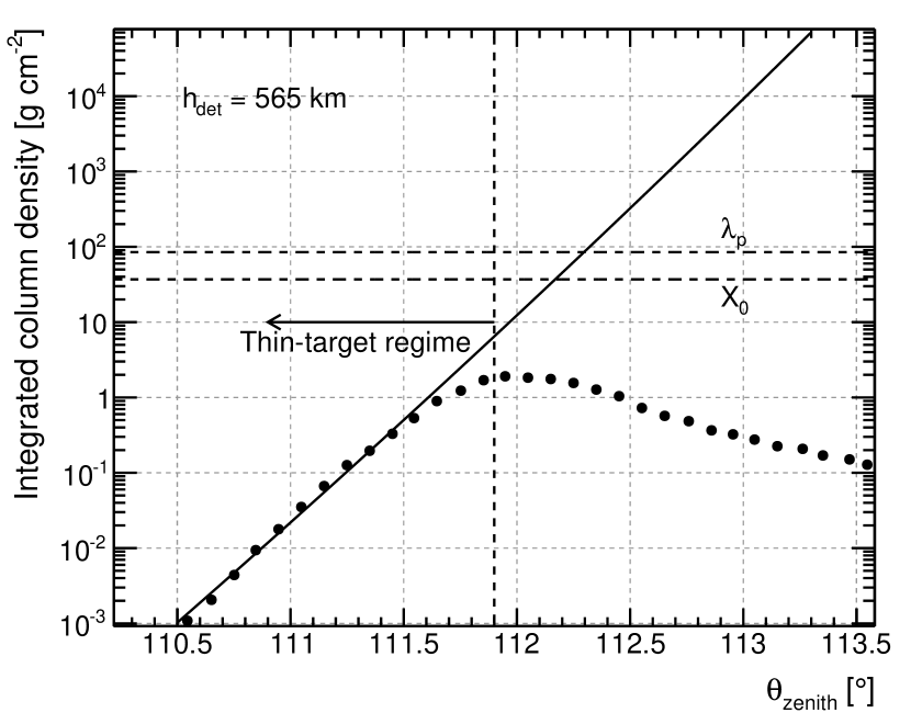
Figure 21: Integrated atmospheric column density, as a function of the zenith angle, for a detector in orbit at 565 km altitude (i.e., a la Fermi). The calculation is based on a simple isothermal model of the atmosphere with a scale height of 7 km. The points represent the zenithal profile of the limb emission, deconvolved for the PSF, measured by Fermi above 3.6 GeV, adapted from Abdo et al. (2009), and follows the integrated column density profile in the thin-target regime. (When comparing with Abdo et al. (2009) keep in mind that we are using a different definition of the zenith angle.)

Figure 21 shows the integrated column density as a function of the zenith angle for our naïve isothermal atmospheric model. When its value is less than $\sim 10$ g cm^-2 (i.e., much smaller than the radiation length of the air) we are in the so-call thin-target regime, where gamma-ray production involves a single interaction and the gamma-ray spectrum is tracing that of primary cosmic rays Ackermann et al. (2014). This makes the limb of the Earth an excellent gamma-ray calibration source for instruments in low-Earth orbit (see, e.g., Ackermann et al. (2012c)). For completeness, since the coefficient of in-elasticity of the process is of the order of $k=0.17$, gamma rays of, say, 10 GeV are produced on average by protons of $\sim 60$ GeV.

VI.2 The Earth Magnetic Field

The fact that the Earth generates a magnetic field, and the magnitude of this field is $\sim 0.5$ G, is a notion everybody has been taught in his/her undergraduate education. As it turns out, enormous progress has been made, over the last century or so, in mapping the basic properties of the geomagnetic field.

In the following of this section we shall use spherical coordinates $(r,\theta,\phi)$ centered and aligned with the magnetic dipole generating the lowest-order component of the geomagnetic field. In addition to the magnetic co-latitude $\theta$, we shall also occasionally make use of the magnetic latitude $\lambda=90^{\circ}-\theta$, which is widely used in the literature.

In source-free regions (i.e., above the Earth’s surface), since $\nabla\times{\mathbf{B}}=0$, the static magnetic field can be expressed as the negative gradient of a scalar potential $\psi$, just like the ordinary electrostatic field. This potential, in turn, can be expanded in spherical harmonics as

$$\psi(r,\theta,\phi)= R_{E}\sum_{n=1}^{\infty}\left(\frac{R_{E}}{r}\right)^{n+1}$$

$$\sum_{m=0}^{n}(g_{n}^{m}\cos m\phi+h_{n}^{m}\sin m\phi)P_{n}^{m}(\cos\theta).$$ (24)

(The reader is referred to Walt (1994) for the exact definition of the terms; we limit ourselves to note that, with the expansion written in this form, $g_{n}^{m}$ and $h_{n}^{m}$ have the dimensions of a magnetic field.) Modern professional descriptions of the geomagnetic field, such as the eleventh generation of the International geomagnetic Reference Field (IGRF) contain the coefficients of such expansion up to order 13 Finlay et al. (2010).

VI.2.1 The ideal dipole field

Many of the features of the geomagnetic field can be effectively illustrated by truncating the expansion to the lowest-order (i.e., the dipole) term, with $n=1$ and $m=0$ (which is the same as saying that the Earth’s magnetic field is, to a reasonable approximation, a dipole field):

$$\psi(r,\theta,\phi)=R_{E}\left(\frac{R_{E}}{r}\right)^{2}g_{1}^{0}\cos\theta.$$ (25)

The two non-trivial components of the magnetic field (the component along the $\phi$ versor is identically $0$ for symmetry reasons), read

$$B_{r}(r,\theta,\phi)= -\frac{\partial\psi}{\partial r}=2\left(\frac{R_{E}}{r}\right)^{3}g_{1}^{0}\cos\theta,$$

$$B_{\theta}(r,\theta,\phi)= -\frac{1}{r}\frac{\partial\psi}{\partial\theta}=\left(\frac{R_{E}}{r}\right)^{3}g_{1}^{0}\sin\theta,$$ (26)

i.e., the field is purely radial at the poles and purely tangential at the equator. For completeness, the intensity of the dipole field at any given point is given by

$$B(r,\theta,\phi)= \sqrt{B_{r}^{2}(r,\theta,\phi)+B_{\theta}^{2}(r,\theta,\phi)}=$$

$$= \left(\frac{R_{E}}{r}\right)^{3}g_{1}^{0}\sqrt{1+3\cos^{2}\theta}.$$ (27)

From the above expression it is easy to recognize that physically $g_{1}^{0}$ represents the field intensity $B_{0}$ at the equator ($\theta=90^{\circ}$) on the Earth’s surface ($r=R_{E}$). It is also easy to recognize that the field intensity on the Earth’s surface is minimum at the equator and twice as large at the magnetic poles.

Even more important, it follows from (VI.2.1) that the equation for a geomagnetic field line, is

$$\frac{1}{r}\frac{{\rm d}r}{{\rm d}\theta}=\frac{B_{r}}{B_{\theta}}=\frac{2\cos\theta}{\sin\theta},$$ (28)

which is readily integrated to give the equation of the field lines:

$$r=R_{E}L\sin^{2}\theta.$$ (29)

(Mind when you do that you have logarithms on both sides that simplify.) At this point the quantity $L$ in the equation above (which is customarily referred to as the McIlwain $L$ coordinate) is just a constant of integration, but one with a pretty straightforward physical interpretation—it is the distance, measured in units of Earth’s radii, at which a given field line crosses the magnetic equator ($\theta=90^{\circ}$). For completeness, the McIlwain $L$ coordinate can be expressed in term of the geomagnetic coordinates as

$$L=\frac{r}{R_{E}\sin^{2}\theta}=\frac{r}{R_{E}\cos^{2}\lambda},$$ (30)

which becomes

$$L=\frac{1}{\sin^{2}\theta}=\frac{1}{\cos^{2}\lambda}$$ (31)

on the surface of the Earth ($r=R_{E}$). (Note that for an ideal dipole the field is azimuthally symmetric and the McIlwain $L$ coordinate does not depend on $\phi$.)

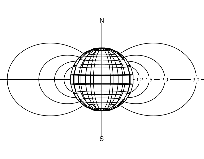
Figure 22: Basic sketch of the field lines (or L-shells) for a centered and aligned dipole field. The numbers indicate the McIlwain $L$ coordinate (i.e., the distance from the dipole center to the intersection with the equator, measured in units of Earth’s radii) for each shell.

Figure 22 shows some illustrative geomagnetic field line in our dipole approximation. Each of those line defines, by rotation in the $\phi$ coordinate, a shell intersecting the equatorial plane at a given distance from the dipole center. By definition all the points on such a shell have the same McIlwain $L$ coordinate (for instance, the points at $L=2$ are those on the magnetic field lines intersecting the equator at $2$ Earth radii). As we shall briefly see in section VI.2.6, the McIlwain $L$ coordinate is convenient to describe the population of trapped particles in the Earth’s magnetosphere (see, however, Pilchowski et al. (2010) for a succinct account of some of the subtleties involved in the definition of the McIlwain $L$ coordinate for non-dipolar field geometries).

We note, in passing, that the field magnitude is not constant along the field lines, so that, strictly speaking, different points on the same $L$-shell are not magnetically equivalent. In fact the field intensity decreases monotonically with the co-latitude $\theta$ along a field line

$$B(\theta)=\frac{B_{0}}{L^{3}}\frac{\sqrt{1+3\cos^{2}\theta}}{\sin^{6}\theta}.$$ (32)

The $B$ coordinate defined by the above equation provides an obvious parameterization of the geomagnetic environment within each given $L$ shell and the McIlwain $(B,~{}L)$ coordinates are widely used to describe the motion of slow charged particles in the Earth’s magnetic field.

VI.2.2 The actual geomagnetic field

The actual geomagnetic field is not a perfectly aligned and centered dipole. First of all the dipole axis is misaligned by $\sim 11^{\circ}$ with respect to the spin axis of the Earth. In addition, the center of the dipole does not coincide with the center of the Earth (the offset being of the order of 700 km). Finally, asymmetries in the interior current system generating the magnetic field produce higher-order terms in the expansion (VI.2).

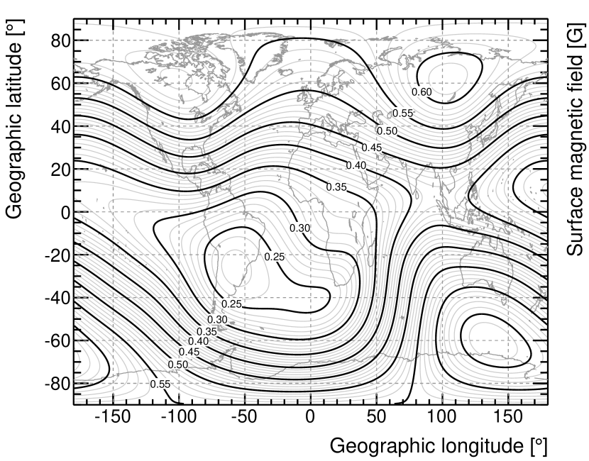
Figure 23: Iso-contours of the Earth’s magnetic field, in G, at sea-level. The data have been taken from the IGRF-11 model. (For completeness, the reference time is January 1, 2013.)

Figure 23 shows a typical map of the intensity of the magnetic field at the Earth’s surface. If our ideal dipole approximation was a perfect description of reality, the iso-intensity lines would be parallel to the equator (i.e., there would be no $\phi$ dependence) and the intensity at the poles would be exactly twice that at the equator. Figure 23 gives a fairly good idea of the departure of the geomagnetic field from the simplistic dipole approximation.

That all said, the McIlwain parameterization of the geomagnetic environment is a useful concept even in the real geomagnetic field. Figure 24 shows a map of the McIlwain $L$ iso-intentity lines at an altitude of $500$ km above the sea level (i.e., in low-Earth orbit). Again, in the dipole approximation those lines would be parallel to the equator.

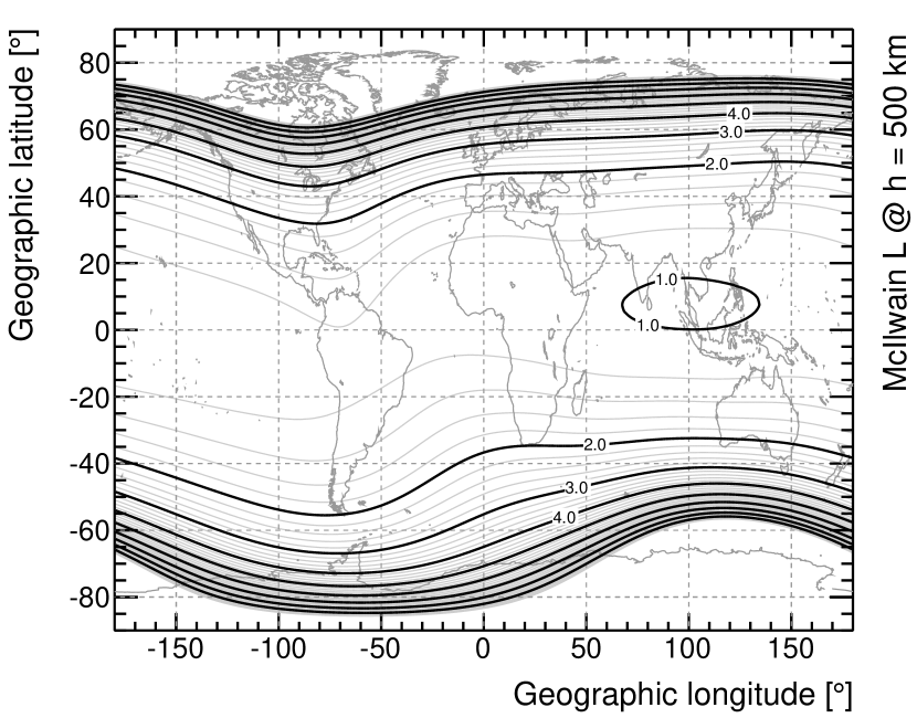
Figure 24: Iso-intensity line of the McIlwain $L$ parameter at an altitude of $500$ km for the same field model shown in figure 23. (For completeness, the reference time is January 1, 2013.)

VI.2.3 Ray-tracing techniques

Computer programs exists that, given a detailed model of the geomagnetic field (e.g., the aforementioned IGRF model) allow to numerically solve the classical equations of motion and provide reliable predictions for the actual trajectories of charged particles, as illustrated in figure 25. The reader is referred to Walt (1994) for an elementary introduction to the motion of charged particles in the geomagnetic field and to Smart and Shea (2005) for a brief overview of numerical ray-tracing techniques.

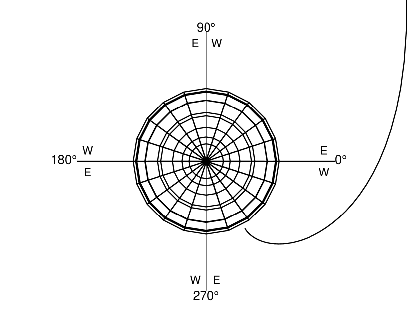
Figure 25: Numerical ray-tracing of an outgoing (i.e., traveling counter-clockwise) 12 GV antiproton in the geomagnetic field. The particle is generated at an altitude of 500 km over the magnetic equator, at a magnetic longitude of $-60^{\circ}$, and the initial momentum is directed along the local zenith. The trajectory is also representative of an in-going (i.e., traveling clockwise) 12 GV proton coming from infinity.

Figure 25 deserves a somewhat detailed description, as we shall encounter several similar instances in the rest of the section—and since, when dealing with the motion of charged particle in a magnetic field, it is easy to get confused with the signs. The sphere represents the Earth viewed from the top, with the geomagnetic North pole at the center of the image. In this representation the geomagnetic field is directed perpendicularly out of the page, so that positively charged particles travel clockwise and negatively charged particles travel counter-clockwise—if you’re not persuaded try it yourself applying the right-hand rule to the expression for the Lorentz force

$$\mathbf{F}=q\mathbf{v}\times\mathbf{B}.$$

In applications where one is interested in the properties of the cosmic-ray particle populations at a given point in the magnetosphere (e.g., the point where the detector is placed) it is not practical to simulate an isotropic flux coming from large distances and select the particles that happen to arrive in the vicinity of the region of interest—that would be way too inefficient. It is customary, instead, to generate particles with the opposite charge at the location of the detector and propagate them to infinity. When doing that, at relatively low energies, it does happen that part of the trajectories intersect the surface of the Earth or end up deep in the atmosphere. These trajectories are called forbidden trajectories as a primary cosmic ray cannot reach the Earth from large distances along any of them. In the following we shall see several examples were the concept of allowed and forbidden trajectory is important.

VI.2.4 The geomagnetic cutoff

The geomagnetic field effectively acts like a shield for (relatively) low-energy charged primary cosmic rays impinging on the Earth. The field being strongest at the magnetic poles, one might naivëly think that the shield effect is stronger there than at the equator. In fact is quite the opposite, as the field at the poles is radial and charged particles coming from the zenith direction can travel unaffected along the field lines. At the equator, on the other hand, the field is orthogonal to the zenith direction and the shielding effect is maximum.

A widely used concept is that of the vertical rigidity cutoff, i.e. the minimum rigidity that is required for a charged particle to reach a point above the Earth surface, at a given altitude, from the direction of the local zenith. Phrased in a different way, for any given geographic position and altitude, particles below the vertical rigidity cutoff from the local zenith direction are effectively shielded by the geomagnetic field.

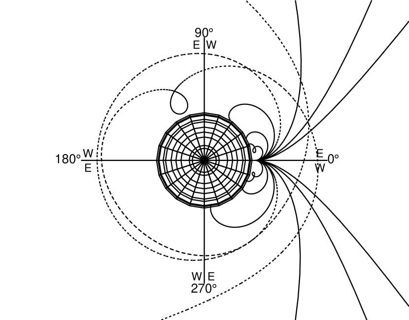
Figure 26: Illustration of the vertical rigidity cutoff numerical calculation. The solid lines corresponds to the trajectories of electrons and positrons with rigidity of $25$, $20$, $15$, $10$, $7.5$ and $5$ GV, starting from a point $500$ km above the equator at a magnetic longitude of $0^{\circ}$ (for completeness, positrons are coming in from the East direction and electrons are coming from the West). The two dashed lines correspond to the rigidity values separating the trajectories reaching out to infinity (allowed) and those intersecting the Earth’s atmosphere (forbidden). These values signal the vertical rigidity cutoff for electrons and positrons.

Strictly speaking, the rigidity cutoff can only be calculated through a full numerical particle tracing in a detailed model of the Earth’s magnetic field. As anticipated in the previous section, the basic strategy to calculate the rigidity cutoff for, say, electrons at a given position is to simulate the trajectories of positrons moving out from the very same position in the direction of the local zenith for several different rigidity values. The rigidity separating allowed and forbidden trajectories defines the vertical rigidity cutoff, as illustrated in figure 26.

As it turns out, however, in a dipolar geomagnetic field approximation the equations of motion of a charged particle can be analytically integrated Smart and Shea (2005) to get an explicit expression for the vertical rigidity cutoff

$$R_{v}=\frac{R_{0}\sin^{4}\theta}{r^{2}}=\frac{R_{0}\cos^{4}\lambda}{r^{2}}=\frac{R_{0}}{L^{2}},$$ (33)

with $R_{0}=14.5$ GV. Figure 27 shows the iso-intensity contours of the vertical rigidity cutoff at an altitude of $500$ km. Near the equator the typical cutoff value is of the order of $\sim 15$ GV, while sub-GV values can be reached moving close to the magnetic poles.

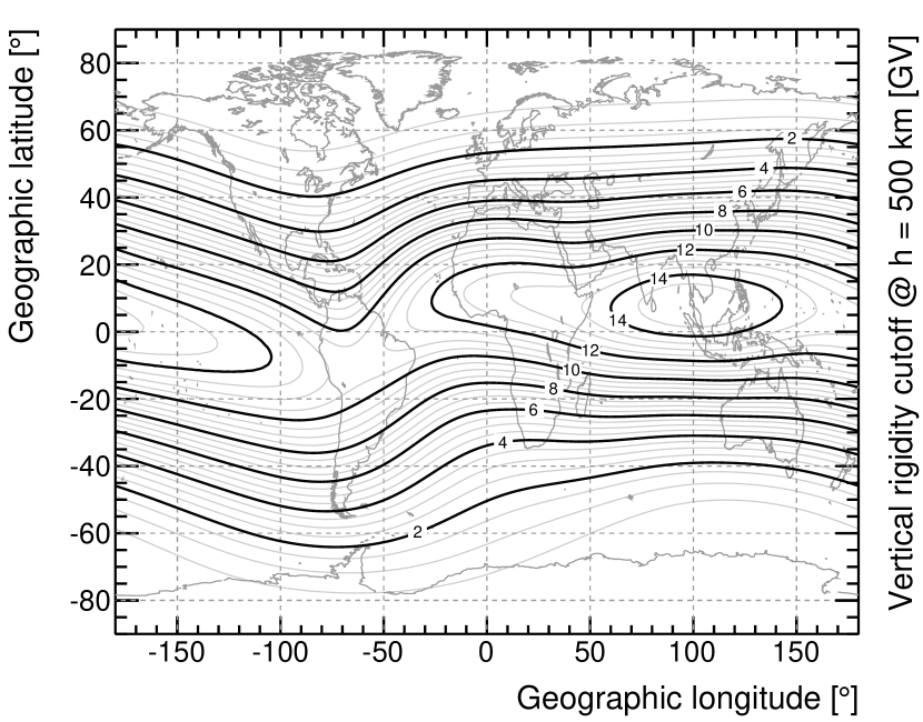
Figure 27: Iso-intensity lines of the vertical rigidity cutoff, in GV, at an altitude of $500$ km for the same field model shown in figure 23.

We stress that this is not only relevant if one aims at measuring primary cosmic rays down to the lowest possible energies, as in any event it has practical implications on the level of backgrounds and the overall trigger rates. We also note, in passing, that while balloon-borne experiments operate at roughly constant McIlwain $L$ (and rigidity cutoff), satellite experiments orbiting at a fixed inclination span a range of L values and therefore have variable background and trigger rate as a function of the position in the orbit.

VI.2.5 The East-West effect

As mentioned in section V.1, Bruno Rossi predicted early in the 1930s that, if the primary cosmic rays carry predominantly one charge sign (and we know that the vast majority of primary cosmic rays are positively charged), one should observe an East-West flux asymmetry—which is maximal around the geomagnetic equator.

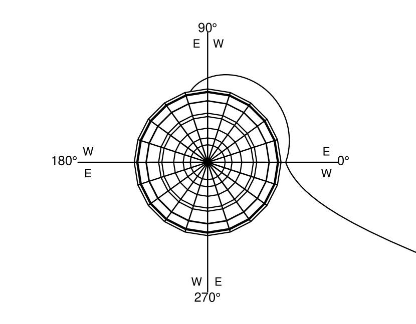
Figure 28: Illustration of the East-West effect. The figure shows the trajectories of two 30 GV protons reaching a point 500 km above the geomagnetic equator at $0^{\circ}$ geomagnetic longitude and a zenith angle of $70^{\circ}$. The trajectory coming from the East direction is forbidden (i.e., protons from this direction are effectively shielded), while that from the West direction is allowed.

The effect is sketched in figure 28, where the trajectories of two 30 GV protons incoming from the East and the West directions are shown. In the first case the trajectory intersects the Earth’s surface and is therefore forbidden—it cannot possibly represent a primary proton coming from infinity. On the other hand the trajectory from the West is allowed. As the rigidity increases the trajectories get more and more straight and the magnitude of the effect tends to vanish, but there is a relatively large energy range, between a few GV and a few tens of GV, where the shadow of the Earth tends to suppress the flux of positively charged particles coming from the East. Since the primary cosmic-ray spectrum is a steep power law, this has a prominent effect of the integral flux.

We shall see in section VI.2.8 that the same kind of effect can be used, at least to some extent, to distinguish the charge sign by means of instrument that are not equipped with a magnet.

VI.2.6 Secondary radiation in low-Earth orbit

Below the geomagnetic cutoff primary cosmic rays are reprocessed by the combined effect of the geomagnetic field and the atmosphere of the Earth. While this is not really the focus of this review, the subject is relevant for all space-based instruments, as the sub-cutoff particle populations can have a major impact on the trigger rate and constitute an important source of background—especially for gamma-ray detectors.

The basic theory of geomagnetically trapped radiation is thoroughly discussed in Walt (1994) (and Lipari (2002) is another good source of information). Trapped particles are generated by the interaction of primary cosmic rays with the atmosphere and generally undergo a characteristic bouncing motion around the geomagnetically field lines between two mirror points (placed symmetrically with respect to the geomagnetic equator), with a contestual drift in the azimuthal direction, before being re-absorbed in the atmosphere. The number of times a particle bounces back and forth between the mirror points determines its trapping time, with the radius of the Earth determining the minimum timescale $R_{E}/c\sim 20$ ms. Figure 29 illustrates the bouncing and drift motion characteristic of the trapped radiation. It should be noted that it takes place on a fixed McIlwain $L$ shell, which is the basic reason why the McIlwain $L$ coordinate is a useful concept from the standpoint of studying the trapped radiation.

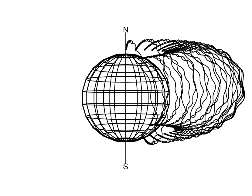
Figure 29: Trajectory of a $1$ GeV proton starting at an altitude of $2000$ km. The figure illustrates the complex motion of the low-energy trapped radiation, bouncing back and fourth multiple times between the magnetic mirror points.

While a detailed description of all the salient characteristics of the trapped radiation (in terms of geographical distribution, energy spectra and chemical composition) is way beyond the scope of this paper, we do mention here a striking feature—namely the fact that the positron ratio (i.e., the ratio between the $e^{+}$ and the $e^{+}+e^{-}$ intensity) is much higher than that of primary cosmic rays. As a matter a fact sub-cutoff positrons can outnumber electrons by a factor of $\sim 4$. This can be readily understood by noting that trapped radiation is mostly injected in the magnetosphere by primaries impinging tangentially on the atmosphere, as the lower-energy secondary products of the interactions are beamed in the forward direction due to momentum conservation and are immediately absorbed in the atmosphere if the primary is impinging radially. Now: if the primary cosmic ray is impinging from the west, positively-charged secondaries (e.g., positrons) are deflected away from the atmosphere by the magnetic field, while negatively-charged ones (electrons) are deflected toward the atmosphere and readily absorbed. In other words primary cosmic rays from the West preferentially inject positrons in the magnetosphere. For particles impinging from the East direction it’s exactly the opposite—but they are less numerous due to the East-West effect.

Figure 30 shows the cosmic-ray electrons and positron spectra around the cutoff (i.e., around the transition between the trapped population and the primary cosmic rays) measured by the Fermi Large Area Telescope in several bins of McIlwain $L$. We shall see in section XI.2.3 how this can be exploited for an in-flight calibration of the absolute energy scale.

Figure 30: Inclusive cosmic-ray electron spectrum as measured by the Fermi Large Area Telescope in bins of McIlwain $L$ (adapted from Ackermann et al. (2010)). For each of the series of data point the peak-like structure is given by the convolution of the primary power-law spectrum and the geomagnetic rigidity cutoff—averaged over a relatively wide range of $L$ values and zenith angles. Below the cutoff the spectrum is that of the trapped positron and electrons.

VI.2.7 The South Atlantic Anomaly

The South Atlantic Anomaly (SAA) is the region where the radiation belts comes closest to the Earth’s surface—down to an altitude of $\sim 200$ km. Interestingly enough, the radiation belts are, generally speaking, not terribly relevant for instruments in low-Earth orbit, as their intensity tends to be maximum at much higher altitudes. The SAA, roughly located above Brazil, is a notable exception. The level of radiation in the SAA can exceed by orders of magnitude that in other regions at the same altitude—at the level that space-based instruments may have to interrupt ordinary data taking during the SAA passages (this is the case, e.g., for Fermi, which spends some $\sim 15\%$ of the time in the SAA).

VI.2.8 Separating charges using the geomagnetic field

The geomagnetic field can be used, under certain conditions, to distinguish the charge sign without making use of a magnetic spectrometer. As illustrated in figure 31, for any given energy, position and altitude above the Earth’s surface, one can define specific regions, in zenith/azimuth coordinates, where only primaries with positive or negative charge are allowed. More specifically, there exists a region toward the East where only negative charges (e.g., electrons) are allowed and a similar (but not exactly specular) region toward the West where only positive charges (e.g., positrons) are allowed. These regions become smaller and smaller as the particle energy increases, up to the point where the angular resolution of the instrument becomes the limiting factor—determining the upper limit of the energy range where the measurement is practically feasible.

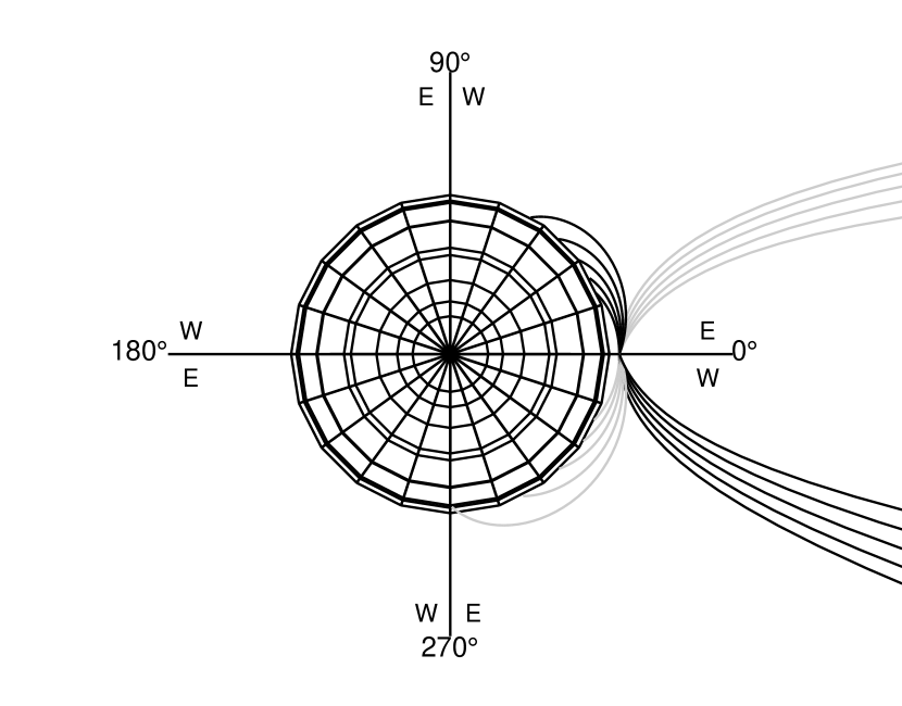
Figure 31: Sample trajectories of 25 GV in-going electrons (in gray) and positrons (in black) on the geomagnetic equatorial plane. For any given energy, position and altitude above the Earth’s surface well defined regions can be defined in zenith/azimuth coordinates where only one charge sign is allowed.

The basic idea dates back to the late 1960s Daniel and Stephens (1965) and has effectively been used to determine the positron fraction between 10 and 20 GeV using the difference in geomagnetic cutoff for positrons and electrons from the East and West Mueller and Tang (1987). More recently the Fermi-LAT has used the same principle, exploiting a full particle ray-tracing in the geomagnetic field, to measure the separate electron and positron spectra between 20 and 200 GeV Ackermann et al. (2012a). Instruments planned for the near future are apparently planning to exploit the same principle Rauch (2014).

We note, in passing, that this concept is more easily applied to separate electrons and positrons, as opposed to, e.g., protons and antiprotons, because one needs an accurate energy measurement to propagate the particle into the geomagnetic field (and, as we shall see in section VIII.4.2 that hadronic calorimetry is a challenging business).

VII Interaction of radiation with matter

This section does not contain more information (and in fact it contains a lot less information) that any of the excellent references floating around Beringer et al. (2012); Leo (1994); Knoll (2010)—except maybe for the fact that we made an effort to put this information in the specific context of the review.

VII.1 Charged particles: energy losses

Energy losses of charged particles are customarily discussed separately for heavy (e.g., protons, alpha particles and nuclei) and light (e.g. electrons) particles—the reason behind that being that radiation losses are, generally speaking, negligible for the the former. Given that, in principle, all particles—be they heavy or light—suffer both ionization and radiation losses, here we take a slightly different approach, focusing our discussion, at the top level, on the distinction between these two types of losses.

VII.1.1 Ionization losses

Relativistic charged heavy particles passing through matter loose energy by ionization at an average rate that is reasonably well described by the Bethe equation over most of energies we are interested:

$$-\left<\frac{dE}{dx}\right>_{\rm ion}\!\!\!\!\!\! =4\pi N_{A}r_{e}^{2}m_{e}c^{2}z^{2}\frac{Z}{A}\frac{1}{\beta^{2}}\times$$

$$\left[\frac{1}{2}\ln\frac{2m_{e}c^{2}\beta^{2}\gamma^{2}T_{\rm max}}{I^{2}}-\beta^{2}-\frac{\delta(\beta\gamma)}{2}\right]$$ (34)

(here $z$, $\beta$ and $\gamma$ refer to the projectile, while $Z$ and $A$ refer to the target material; see Beringer et al. (2012) for a detailed description of all the other terms in the equation).

Complicated as this might seem, the main features are readily evident if one rewrites it as

$$-\left<\frac{dE}{dx}\right>_{\rm ion}\!\!\!\!\!\!\propto z^{2}\frac{Z}{A}\frac{1}{\beta^{2}}\left[\frac{1}{2}\ln(C_{0}\beta^{2}\gamma^{2})-\beta^{2}+\text{corrections}\right].$$ (35)

The energy loss per unit length is proportional to the $Z/A$ ratio of the target material and the square of the charge $z$ of the incident particle. When the latter is slow ($\beta\ll 1$) the energy losses decrease as $1/\beta^{2}\propto 1/E$ as $\beta$ increases. In the ultra-relativistic regime ($\beta\approx 1$) the losses increase as $\ln\beta^{2}\gamma^{2}$ (this generally goes under the name of relativistic rise or logarithmic raise). These basic facts are customarily used, as we shall briefly see in the following, for charge measurement and/or particle identification.

We should note that, since ionization losses are fundamentally due to interactions between the incoming particle and the atomic electrons of the medium, there are significant kinematic differences between the two cases of heavy and light projectiles. In addition to that, quantum-mechanical effects due to the fact that the projectile and the target are identical particles come into play in case of electrons. But we are neglecting a whole lot of details anyway and won’t push this any further.

Figure 32: Average energy loss $dE/dx$, as a function of $\beta\gamma$ for muons in silicon. The data points are taken from http://pdg.lbl.gov/2012/AtomicNuclearProperties/MUON_ELOSS_TABLES/muonloss_014.dat.

When plotted as a function of $\beta\gamma$ (i.e., the momentum) of the incident particle, the energy-loss curve has the typical shape shown in figure 32, with a relatively broad minimum at $\beta\gamma\sim 3$, where $dE/dx$ (normalized to the density of the target) is of the order of 1–2 MeV g^-1 cm². A particle with the energy corresponding to this minimum ionization is customarily called a minimum ionizing particle (MIP).

VII.1.2 Radiation losses and critical energy

At sufficiently high energy any charged particle radiates. Radiation losses are nearly proportional to the particle energy

$$-\left<\frac{dE}{dx}\right>_{\rm rad}\!\!\!\!\!\!\propto E,$$ (36)

and, since ionization losses only grow logarithmically, the two loss rates, when seen as function of energy, are bound to cross each other at some point, as shown in figure 32. The energy $E_{c}$ at which this happens is called critical energy. Since the constant of proportionality in equation (36) scales as $1/m^{2}$, for any given material $E_{c}$ is different for different particles—and it is much higher for heavier particles. For reference, the critical energy in silicon is $\sim 580$ GeV for muons and $\sim 40$ MeV for electrons (and in the tens to hundreds of TeV for protons).

To all practical purposes radiation losses are mainly relevant for electrons (and positrons) and it is customary to refer to the critical energy for electrons as the critical energy. A popular empirical approximation for $E_{c}$ as a function of the atomic number of the material (for solids) is given by

$$E_{c}=\frac{710}{Z+0.92}\ {\rm MeV}$$ (37)

and plotted in figure 33.

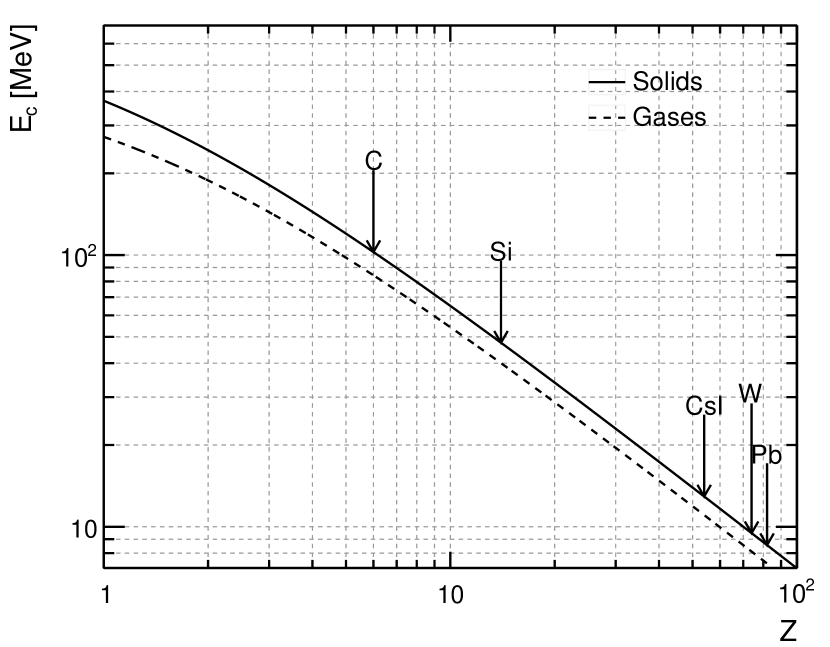
Figure 33: Empirical parameterization of the electron critical energy as a function of the atomic number from Beringer et al. (2012).

VII.1.3 Radiation length

Above the critical energy (i.e. in the regime where radiation losses dominate) equation (36) can readily integrated in a homogeneous material, yielding the electron energy as a function of the distance $x$ traversed:

$$E(x)=E_{0}\exp\left(-\frac{x}{X_{0}}\right).$$ (38)

The quantity $X_{0}$, representing the typical length over which an electron looses all but $1/e$ of its energy due to bremsstrahlung, is called radiation length and is characteristic of the material. The radiation length is conveniently expressed in g cm^-2, i.e., factoring out the density of the medium. A popular parameterization is given by

$$X_{0}=\frac{716A}{Z(Z+1)\ln(287/\sqrt{Z})}~{}{\rm g\ cm^{-2}}$$ (39)

and table 5 shows numerical values for a few materials of interest (see also figure 37).

Material	$X_{0}$ [g cm-2]	$\varrho$ [g cm-3]	$X_{0}$ [cm]
Pb	6.37	11.350	0.561
BGO	7.97	7.130	1.12
CsI	8.39	4.510	1.86
W	6.76	19.3	0.350
C (graphite)	42.70	2.210	19.3
Si	21.82	2.329	9.37
Air	36.62	$1.2\times 10^{-3}$	30,500

Table 5: Tabulated values of the radiation length for some materials of interest.

The radiation length is the natural scale for all the most relevant electromagnetic phenomena we shall deal with in the following: multiple scattering, electron bremsstrahlung, pair production and electromagnetic showers. We shall customarily indicate with the letter $t=x/X_{0}$ any distance measured in units of $X_{0}$.

VII.2 Multiple Coulomb scattering

A charged particle traversing a medium undergoes multiple Coulomb scatterings on the atomic nuclei of the material. In the so-called gaussian approximation the root mean square of the deviation angle projected in any of the planes containing the incoming particle direction can be parameterized as

$$\theta_{\rm MS}^{\rm plane}=\frac{0.0136~{}{\rm GeV}}{\beta cp}z\sqrt{t}(1+0.038\ln t)~{}\text{rad},$$ (40)

where $\beta c$, $p$ and $z$ are the velocity, momentum and charge number of the incoming particle, and $t$ is the thickness of the traversed material in units of radiation lengths.

The deflection space angle being the sum in quadrature of the independent deflections on two orthogonal planes, it is simply given by

$$\theta_{\rm MS}^{\rm space}=\sqrt{2}\theta_{\rm MS}^{\rm plane}.$$ (41)

Whether one or the other is more relevant depends on the problem at hand (e.g., typically the pointing accuracy of a detector is parameterized in terms of the space angle, but in a magnetic spectrometer the important figure is really the deflection angle in the bending plane). In the following we shall use both and we shall try and make clear which one we are referring to.

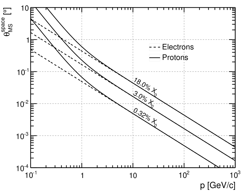
Figure 34: Multiple scattering angle, as a function of the momentum of the incoming particle, for three sample values of $t$, for electrons and protons. The three values of $t$ corresponds to $300~{}\mu$m of silicon (the thickness of the AMS-02 silicon detectors) and the Fermi-LAT thin and thick radiators.

Figure 34 shows the (space) multiple scattering deflection angles for three sample values of $t$, for electrons and protons, as a function of their momentum. In the ultra-relativistic regime $\beta\approx 1$ (i.e. above a few MeV for electrons and above a few GeV for protons) the curves are indistinguishable and fall as $1/p$. The difference below 1 GeV has implication for the momentum resolution in a magnetic spectrometer and we shall come back to it in section IX.4.3.

VII.3 High-energy photons

High-energy photons (above a few tens of MeV) interact with matter mainly by pair production in the field of atomic nuclei. As it turns out, the processes of electron bremsstrahlung and pair production are intimately related to each other, and the mean free path for pair production for a high-energy photon is given by

$$\lambda_{\rm pair}=\frac{9}{7}X_{0}$$ (42)

(i.e., it is $9/7$ of the scale length over which a high-energy electron looses all but $1/e$ of its energy).

It should be noted that, while pair production is a destructive process (the gamma-ray no longer exists afterwards), bremsstrahlung only degrades the electron energy. As we shall see in a second, these two physical processes are at the base of the development of electromagnetic showers.

VII.3.1 More on the pair production

The $e^{+}/e^{-}$ pair production by high-energy gamma rays is the basic physical process used in pair conversion telescopes. It is pretty much conventional wisdom that the kinematic of the process is closed and the tracks of the electron and the positron can in principle be combined to recover exactly the original photon direction. It turns out that, even neglecting the finite detector resolution, this is not quite true, and there are a few subtleties involved that we briefly mention in this section.

The average opening angle of the electron-positron pair scales as

$$\theta_{\rm open}\propto\frac{m_{e}c^{2}}{E},$$ (43)

where $E$ is the photon energy. Depending on $E$ and on the layout of the tracking detectors, this angle might be too small to be resolved, in which case the two tracks effectively overlap (i.e., from an experimental standpoint, one really sees one track).

At low enough energy, where the opening angle is relatively large and the tracks are well separated, in order to recover the original photon direction one should in principle combine the momenta of the two particles covariantly which brings up the question of the track energies. The differential distribution in the fractional electron (or positron) energy is relatively flat so that asymmetric (energy-wise) pairs are quite common—if you think about, this implies that the average energy of the particle in the pair with the highest energy is approximately $3/4$ of the original photon energy. Now, depending on the experimental setup, one might measure the single track energies with good or bad resolution—or just not measure them at all. As one might imagine, this has profound implications on the maximum attainable angular resolution for pair conversion telescopes.

There is one last ingredient to the mix that we haven’t mentioned yet, namely the nucleus recoil (remember, typically gamma rays pair-produce in the field of the nucleus). In practical applications this is largely irrelevant, as one is usually limited by the multiple scattering in the low-energy regime, as we shall see in section IX.5.1. When this is not true the nucleus recoil (which is essentially impossible to measure) becomes the ultimate limiting factor to the accuracy with which one can reconstruct the photon direction. It is shown in Hunter et al. (2014) that this kinematic limit $\theta_{\rm kl}$ is approximately given by

$$\theta_{\rm kl}\sim 5^{\circ}\left(\frac{10~{}{\rm MeV}}{E}\right)$$ (44)

and this figure is possibly relevant when designed gamma-ray detectors optimized for the low-energy end of the pair production regime.

VII.4 Electromagnetic showers

As explained in the previous section, high-energy electrons and photons produce in matter secondary photons by bremsstrahlung and electron-positron pairs by pair production. These secondaries, in turn, can produce other particles with progressively lower energy and start an electromagnetic shower (or cascade). The process continue until the average energy of the electron component falls below the critical energy of the material—at which point the rest of the energy is released via ionization.

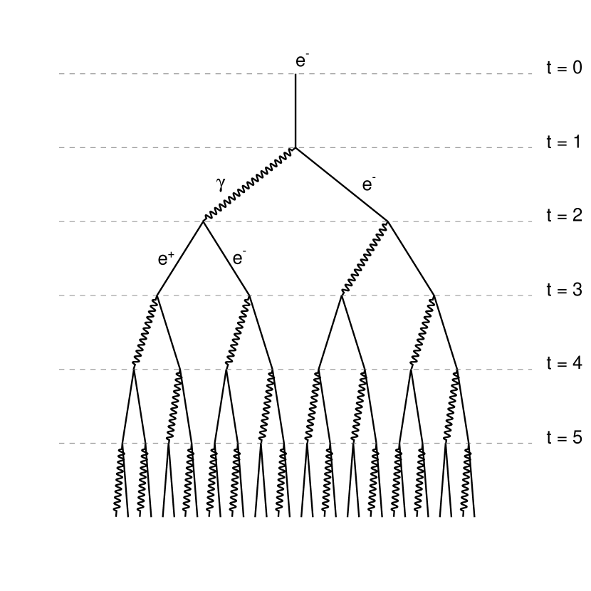
Figure 35: Sketch of the development of an electromagnetic shower in the simplest possible toy model.

A simple toy model for an electron-initiated shower is schematically represented in figure 35, where after $t$ radiation lengths of material, the cascade has developed in $2^{t}$ particles (a mix of electrons, positrons and photons) with average energy $E_{0}/2^{t}$. Rough as this model is (for one thing we neglect the stocasticity of the process altogether, along with the $9/7$ in (42) and the fact that the electron can—and does—radiate multiple photons of different energy per radiation length) it is able to reproduce one of the main features of electromagnetic showers, namely the fact that the position of the shower maximum scales logarithmically with the energy. In fact the stop condition reads

$$\frac{E_{0}}{2^{t_{\rm max}}}\sim E_{c},$$ (45)

and hence

$$t_{\rm max}\sim\ln\left(\frac{E_{0}}{E_{c}}\right).$$ (46)

At a slightly higher level of sophistication, the longitudinal profile of an electromagnetic shower can be effectively described as

$$\frac{dE}{dt}=E_{0}b\frac{(bt)^{a-1}e^{-bt}}{\Gamma(a)},$$ (47)

where $a$ and $b$ are parameters related to the nature of the incident particle (electron or photon) and to the characteristics of the medium ($b=0.5$ is a reasonable approximation in many cases of practical interest). The position of the shower maximum occurs at

$$t_{\rm max}=\frac{(a-1)}{b}\approx\ln\left(\frac{E_{0}}{E_{c}}\right)+t_{0}$$ (48)

where $t_{0}=-0.5$ for electrons and $t_{0}=0.5$ for photons. For the sake of clarity, the way one typically uses these relation is to plug $E_{0}$, $E_{c}$ and $t_{0}$ in (48) to find $a$ (assuming $b=0.5$) and then use (47) to describe the longitudinal profile of the shower.

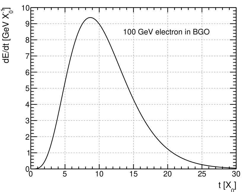
Figure 36: Average longitudinal profile of the shower generated by a $100$ GeV electron in a homogeneous slab of BGO.

Figure 36 shows the average shower profile for $100$ GeV in BGO. With a critical energy of $10.1$ MeV, the position of the shower maximum is located, according to equation (48), at $8.7~{}X_{0}$.

We mention, in passing, that the transverse development of an electromagnetic shower, mainly due to the multiple scattering of electrons and positrons away from the shower axis, scales with the so-called the Molière radius, that can be empirically parameterized as

$$R_{M}\approx\frac{21X_{0}}{E_{c}~{}{[\rm MeV]}}~{}{\rm MeV}.$$ (49)

VII.5 Hadronic showers

While the development of electromagnetic showers is determined, as we have seen, by two well-understood QED processes, the energy degradation of hadrons proceeds through both strong and electromagnetic interactions in the medium. The complexity of the hadronic and nuclear processes produce a multitude of phenomena that make hadronic showers intrinsically more complicated than the electromagnetic ones. In other words for hadronic showers there is no such a thing as the toy model illustrated in figure 35.

As a matter of fact hadronic showers consist in general of two distinctly different components: (i) an electromagnetic component due to $\pi^{0}$ and $\eta$ generated in the absorption process and decaying into photons (which in turn develop electromagnetic showers) before they have a chance to undergo a new strong interaction; and (ii) a non-electromagnetic component, which combines essentially everything else that takes place in the absorption process. Most importantly, the two components evolve with different length scales: the radiation length $X_{0}$ for the first and the nuclear interaction length $\lambda_{I}$ (which is at least on order of magnitude larger for $Z>30$, as shown in figure 37) for the second. A useful parameterization for $\lambda_{I}$ is

$$\lambda_{I}=37.8A^{0.312}~{}\text{g~{}cm}^{-2}$$ (50)

and the actual values for some relevant materials are shown in table 6.

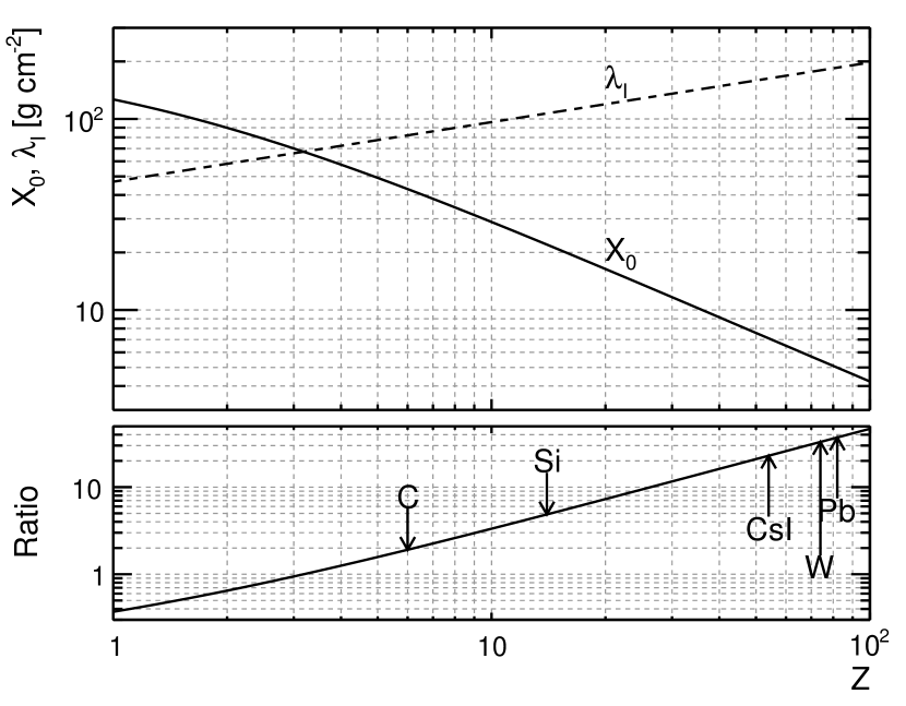
Figure 37: Approximate dependence of the radiation length $X_{0}$ and the nuclear interaction length $\lambda_{I}$ on the atomic number $Z$ of the material. The parameterizations used are those in equations (39) and (50), with the additional assumption $A=2Z$.

Material	$\lambda_{I}$ [g cm-2]	$\varrho$ [g cm-3]	$\lambda_{I}$ [cm]
Pb	199.6	11.350	17.6
BGO	159.1	7.130	22.3
CsI	171.5	4.510	38.0
W	191.9	19.3	9.94
C (graphite)	85.8	2.210	38.8
Si	108.4	2.329	46.5
Air	90.1	$1.2\times 10^{-3}$	75,000

Table 6: Tabulated values of the nuclear interaction length for some materials of interest.

The fractional non-electromagnetic component of a hadronic shower $F_{h}$ (as opposed to electromagnetic component $F_{e}=1-F_{h}$) decreases with energy and is generally Beringer et al. (2012) parameterized as

$$F_{h}(E)=\left(\frac{E}{E_{0}}\right)^{k-1},$$ (51)

where typical values are $E_{0}\approx 1$ GeV and $k\approx 0.8$ (roughly speaking, the fraction of energy the non-electromagnetic component accounts for is of the order of $50\%$ at $100$ GeV and $30\%$ at $1$ TeV).

In broad terms, hadronic showers tend to start developing at relatively large depths in the material and they are typically larger and more irregular when compared with electromagnetic showers. As we shall see in the following, all these differences are customarily used in modern space-based imaging calorimeters for particle identification—particularly to discriminate electrons and photons against the much larger proton background.

VII.6 Cherenkov radiation

Cherenkov radiation is emitted when a charged particle moves in a medium at a speed greater than the speed of light in that medium

$$\beta>\frac{1}{n}.$$ (52)

(Here $\beta$ refers to the incident particle and $n$ is the index of refraction of the material.) In the ideal case of a non-dispersive medium, the Cherenkov wave front form an acute angle with respect to the particle velocity given by

$$\cos\theta_{c}=\frac{1}{n\beta}$$ (53)

as sketched in figure 38.

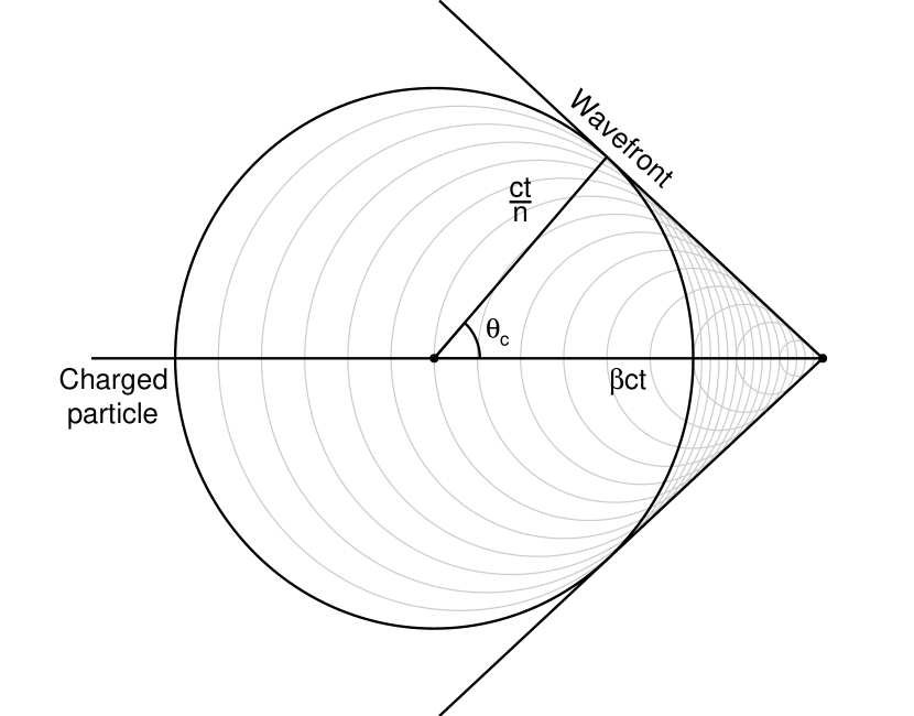
Figure 38: Sketch of the geometry relevant for the Cherenkov effect.

The (double differential) spectrum of the photons produced per unit path length and wavelength is given by

$$\frac{d^{2}N}{dxd\lambda} =\frac{2\pi\alpha z^{2}}{\lambda^{2}}\left(1-\frac{1}{\beta^{2}n^{2}(\lambda)}\right)=$$

$$=\frac{2\pi\alpha z^{2}}{\lambda^{2}}\left(1-\frac{1+\beta^{2}\gamma^{2}}{\beta^{2}\gamma^{2}n^{2}(\lambda)}\right),$$ (54)

where $z$ is the charge of the projectile, and the index of refraction $n$ is evaluated at the generic photon wavelength $\lambda$. Equation (VII.6) cannot be readily translated into a detector signal as, in practice, one has to convolve it with the response of the transducer and integrate over the photon wavelengths of interest. That all said, plotting (VII.6) for a reference value of the index of refraction is a useful illustrative exercise.

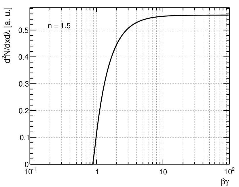
Figure 39: Number of Cherenkov photons emitted per unit path length and wavelength as a function of the $\beta\gamma$ of the projectile, for a reference index of refraction $n=1.5$.

While, strictly speaking, the Cherenkov radiation is generally not important in terms of energy losses, we shall see in the following that its basic properties (the existence of a threshold and the dependence of $\theta_{c}$ and $d^{2}N/dxd\lambda$ on the velocity of the particle) are customarily exploited in high-energy physics for particle identification and velocity measurements. In particular figure 39 shows that the steep slope near the threshold potentially allows to achieve a good velocity or momentum resolution in that region (while the amount of radiation saturates at higher energies).

VII.7 Transition radiation

Transition radiation is emitted when a ultra-relativistic particle crosses the interface between two media with different indices of refraction. As we shall see in the following, in practical implementations the useful (i.e., detectable) photons are in the x-ray band, which requires the incidence particle to have a relativistic $\gamma$ factor of the order of $10^{3}$.

For a single interface the fractional energy emitted into x-rays above a given energy $\hbar\omega_{0}$ is given by

$$F(\hbar\omega>\hbar\omega_{0})=\frac{\alpha z^{2}}{\pi}\left[\left(\ln\frac{\gamma\omega_{p}}{\omega_{0}}-1\right)^{2}+\frac{\pi}{12}\right],$$ (55)

where $\omega_{p}$ is the plasma frequency of the radiation. If $\gamma$ is big enough it effectively scales as

$$F(\hbar\omega>\hbar\omega_{0})\propto z^{2}\ln\gamma.$$ (56)

This form of (55) highlights the two main features of the transition radiation—namely: it scales as $z^{2}$ with the charge of the particle and it grows with $\gamma$.

Since, in practical situations, $F$ is small, transition radiation detectors typically exploit multiple boundary crosses to enhance the signal. In this case interference effects lead to a saturation effect at a value $\gamma$ that, depending on the actual design, ranges from a few $10^{3}$ to $\sim 10^{5}$.

VIII Experimental Techniques

In this section we briefly review some of the most widely used experimental techniques (mind this largely relies on the content of the previous section).

VIII.1 Tracking detectors

The simplest—and yet most widely used in practical implementations—configuration for a tracking stage of a modern experiment is a stack of parallel detection planes. The basic building block of such an instrument is a position-sensitive detector, i.e., a device capable of measuring the position of passage of the particle—in one or both dimensions.

At the top level, the two main figures of merit of a tracking detectors are the tracking efficiency (i.e., the efficiency of correctly reconstructing the track of the incoming particle) and the spatial and/or angular resolution. At a more fundamental level, these performance figure derive largely from the hit efficiency and resolution of the position-sensitive detector used, though in practice there are many more considerations involved (e.g., we shall see in sections IX.5.1 and IX.4.3 two examples of interplay between the hit resolution and the multiple scattering in practical tracking applications.)

Other relevant figures of merit of tracking systems are, in no particular order: triggering capabilities, time response, dead time per event, radiation tolerance, robustness, reliability, power consumption.

VIII.1.1 Position-sensitive detectors

There are literally too many position-sensitive detectors used in tracking applications to list them here, and we refer the reader to Beringer et al. (2012) and references therein for a comprehensive review. Roughly speaking, most tracking detectors exploit the ionization produced by charged particles as they traverse matter. In order for the electron-ion (or electron-hole) pairs not to recombine immediately a suitable electric field is necessary—and drifting under the effect of this electric field the charges induce on the readout electrodes a signal that is generally amplified, processed and digitized by some form of readout electronics.

At a microscopic level, the amount of primary free charge that is created as a particle traverse a medium is determined by the effective ionization energy. This determines the counting statistic of the process and, as a consequence, the energy resolution (in applications where this is relevant). The average ionization energy is smaller, e.g., for semiconductor detectors relative to gaseous detectors, though it should be noted that in the latter case avalanche processes can be exploited to multiply the primary ionization in the detector medium.

The drift velocity of the ionization toward the readout electrodes is another fundamental characteristic of a position-sensitive detector, as it determines the time profile of the charge signal at the input of the readout electronics. In broad terms, gas detectors are generally slower than semiconductor detectors.

The hit efficiency is defined as the efficiency of signaling the passage of a (minimum ionizing) particle and usually runs not too much below $100\%$ within the active area for a decent modern detector. (We note, in passing, that it does not really make sense to quote an efficiency without quoting the corresponding noise level, or the rate of spurious hits. Here we really mean “$\sim 100\%$ hit efficiency at a reasonable noise level” whatever than means in any specific context.) Hit resolutions of $\sim 10~{}\mu$m are not uncommon in modern silicon-strip trackers.

The positional measurement capabilities are usually achieved by segmenting the readout electrode(s), e.g., in strips or pixels. We note, in passing, that the number of readout channels in a pixel detector scales as the square of the active surface (as opposed to strip detectors, for which the scaling is linear), and therefore pixel detectors are not particularly fashionable for use in space due to power constraints (there are, however, exception, see e.g. Park et al. (2007); Zatsepin et al. (2003)). The hit resolution denotes the resolution on the point where the particle hit the detector and it is obviously related to the level of segmentation of the sensor. For a strip detector with pitch $p$ it is given by

$$\sigma_{\rm hit}=\frac{p}{\sqrt{12}}$$ (57)

(i.e., the standard deviation of a uniform continuous distribution) if a single strip is hit and can be significantly better is more strips are hit and the pulse-height information is available to baricenter the position.

VIII.1.2 Silicon detectors

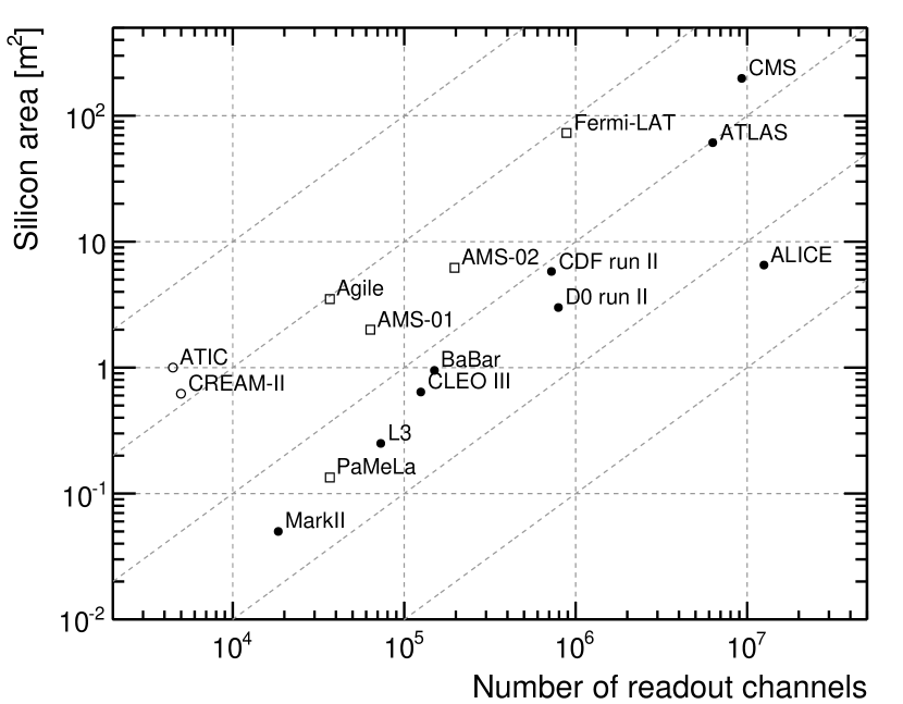
Figure 40: Silicon surface vs. number of readout channels for a compilation of tracking detectors operated at accelerators, in space and on balloons.

Semiconductor detectors—and very especially silicon detectors—are widely used in modern high-energy physics experiments (see figure 40), as integrated circuit technology allows the realization on large scale of high-density electrode structures, with excellent spatial resolution and very fast intrinsic response time. All the last-generation space-based experiments where state-of the-art tracking capabilities are needed exploit silicon (strip, mostly) detectors (see, e.g., table 7). In this section we shall briefly review some of the basic related concepts and we refer the reader to Hartmann (2012) for a comprehensive review of silicon tracking detectors in high-energy physics.

Experiment	Area [m2]	Channels	Pitch [$\mu$m]	Power [W]
AGILE	3.5	36,864	242	15
AMS-02	6.2	196,608	110/208	140
Fermi-LAT	73.0	884,736	228	160
PaMeLa	0.134	36864	50/50	37

Table 7: Main features of some of the silicon trackers built for space-based cosmic-ray and gamma-ray detectors. For the magnetic spectrometers the two figures for the strip pitch indicate the values for the bending/non-bending view, respectively.

Silicon detectors are essentially $p$-$n$ junction diodes operated at reverse bias. The bias voltage has the primary purpose of increasing the depth of the so-called depletion region, defining the active volume of the detector. Full depletion can generally be achieved with 100–200 V bias over a typical thickness of 300–400 $\mu$m.

One of the primary advantages of silicon detectors over other typologies of sensors is the small (3.6 eV) average energy needed to create an electron-hole pair—roughly an order of magnitude less than what is usually required in a gaseous detector. For the same radiation energy this translates, as mentioned in a the previous section, into a corresponding increase in terms of primary charge carriers created. In addition they feature very fast intrinsic response times (of the order of ns) and can be reliably produced with active surfaces of tens (or hundreds) of m². They are self-triggering and do not require consumables (e.g., gas), which makes them ideal candidates for long-term operation in space.

VIII.2 Magnetic Spectrometers

Momentum is typically measured by measuring the deflection of the charged-particle trajectory in a magnetic field. There are actually two slightly different concepts of magnetic spectrometers: those measuring the deflection angle and those measuring the sagitta. While this distinction is partially artificial, the most notable difference is that the tracking detectors are arranged in two arms outside of the deflecting magnet in the first case, while they are placed inside the magnet in the latter. Placing the tracking stage inside the magnet is key to make the spectrometer compact and therefore this is typically the solution adopted in space. We shall see, though, that AMS-02 in the permanent magnet configuration is actually an interesting hybrid between the two concepts.

Figure 41 illustrates the basic principle of a magnetic spectrometer measuring the sagitta. The curvature radius for a particle with charge $z$ (in units of the electron charge $e$) and transverse momentum $p$ (in the following we shall neglect the trivial drift in the longitudinal direction) in a magnetic field $B$ is

$$\rho=\frac{p}{zeB}=\frac{R}{cB}=\frac{R~{}[{\rm GV}]}{0.3B~{}[{\rm T}]}~{}{\rm m}.$$ (58)

In this context the rigidity $R$ is a convenient quantity to work with, as particles with the same rigidity behave the same way in a magnetic field, irrespectively of their charge. If $\rho$ is measured and $B$ is known, one can recover $R$—and, assuming that the charge of the particle is also known, the momentum $p$.

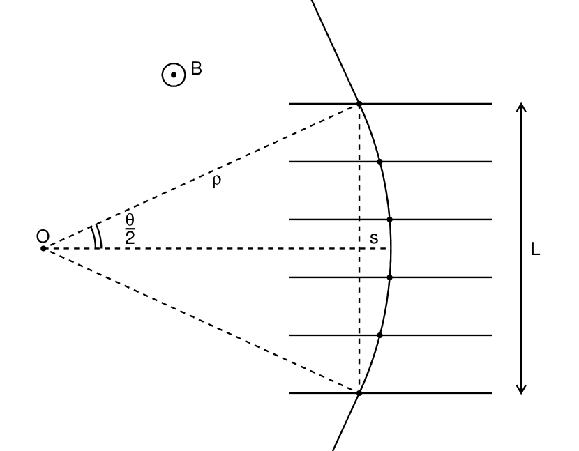
Figure 41: Sketch of the momentum measurement in a uniform magnetic field (in the bending view). Here and in the following of this section $L$ is the height of the region permeated by the magnetic field, $\rho$ is the radius of curvature of the track, $\theta_{\rm B}$ is the deflection angle, and $s$ is the sagitta of the track.

One can see in figure 41 that $L$ and the deflection angle $\theta$ are related

$$\frac{L}{2}=\rho\sin\left(\frac{\theta_{\rm B}}{2}\right)\approx\frac{\rho\theta_{\rm B}}{2}$$ (59)

(the latter holding in small-angle approximation). The bending angle $\theta_{\rm B}$ therefore reads

$$\theta_{\rm B}\approx\frac{L}{\rho}=\frac{cBL}{R}=\frac{0.3B~{}[{\rm T}]~{}L~{}[{\rm m}]}{R~{}[{\rm GV}]}~{}{\rm rad}.$$ (60)

The details of the measurement depend somewhat on the detector setup (e.g., the number of measurements and relative spacing of the tracking planes, not to mention the pattern recognition and track-fitting algorithms) but essentially what we measure is the sagitta $s$ of the trajectory

$$s =\rho\left[1-\cos\left(\frac{\theta_{\rm B}}{2}\right)\right]\approx\frac{\rho\theta_{\rm B}^{2}}{8}\approx\frac{L^{2}}{8\rho}=\frac{cBL^{2}}{8R}=$$

$$=\frac{37.5~{}B~{}[{\rm T}]~{}L^{2}~{}[{\rm m^{2}}]}{R~{}[{\rm GV}]}~{}{\rm mm}.$$ (61)

It goes without saying that the expression we derived is typically used in the opposite direction, i.e., one measures $s$ to deduce $R$:

$$R=\frac{cBL^{2}}{2s}=\frac{37.5~{}B~{}[{\rm T}]~{}L^{2}~{}[{\rm m^{2}}]}{s~{}[{\rm mm}]}~{}{\rm GV}.$$ (62)

The quantity $BL^{2}$ is customarily referred to as the bending power and it is one of the basic figures of merit for a magnetic spectrometer, as it determines the sagitta of the track.

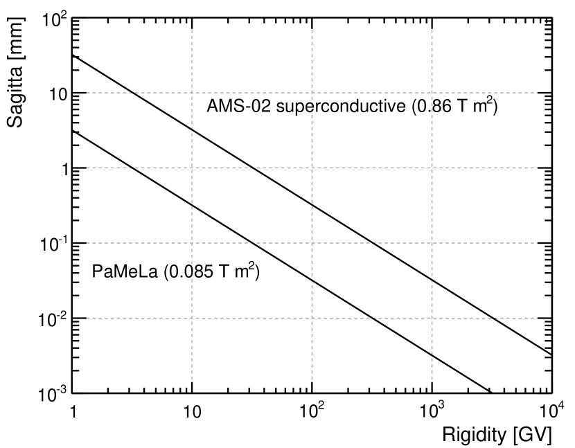
Figure 42: Trajectory sagitta as a function of rigidity (see figure 41). The two lines correspond to two illustrative values of the bending power, corresponding to PaMeLa and the original design of AMS-02—with the superconductive magnet). We have not used the AMS-02 design that is operating on the ISS as the two external tracker planes do not quite fit in our simplified cartoon—and the original AMS-02 design is still representative of the current technological bleeding edge—but we shall come back to that in section IX.4.3. Note that the plot uses the small-angle approximation that might be inaccurate at small rigidity.

Figure 42 shows the value of the trajectory sagitta as a function of the particle rigidity for two representative values of the bending power. At a rigidity of $\sim 1$ TV the track displacement that one aims measuring, with the magnetic field that can be reasonably achieved, is between $\sim 5$ and $\sim 50~{}\mu$m, i.e., at the limit of a typical solid-state tracking detector. We anticipate that this is indeed the limiting factor for the maximum detectable rigidity, and in the high-momentum regime the relative uncertainty on the rigidity increases linearly with the rigidity itself

$$\frac{\sigma_{R}}{R}=\frac{\sigma_{s}}{s}\propto{R},$$ (63)

as the uncertainty on the sagitta $\sigma_{s}$ is a constant dictated by the detector and the sagitta itself $s$ goes like $1/R$. This is one of the most notable differences between spectrometers and calorimeters (see section VIII.4).

VIII.3 Scintillators

Scintillators utilize the ionization produced by charged particles (or by gamma-rays converting into an electron positron pair within the material) into light that can be in turn converted into an electric signal by a photodetector such as a photomultiplier tube (PMT) or a pin diode.

Scintillating materials are broadly divided into organic (most notably, plastic) and inorganic—the main difference being that the first have a relatively low density (and are therefore widely employed, e.g., in trigger, anti-coincidence and time of flight systems), while the latter are used in applications, such as calorimetry (see section VIII.4), where a high stopping power is required.

The choice of a particular material for a particular application is in general dictated by several different properties, such as the light yield, the duration and wavelength spectrum of the output light pulse, the value of the radiation and/or interaction lengths. We refer the reader to Beringer et al. (2012) and reference therein for a more in-depth discussion.

VIII.4 Calorimetry

Calorimeters are instruments in which the particles to be measured are fully or partially absorbed and their energy is transformed into a measurable signal.

Compared to magnetic spectrometers, calorimeters have the double advantage that the energy resolution improves as $1/\sqrt{E}$ at high energy (rather than deteriorating linearly with the particle momentum) and the characteristic dimensions (i.e., the shower depth) scale only logarithmically with the particle energy. In addition, calorimeters are also sensitive to neutral particles and provide position/direction information and particle identification capabilities (though, strictly, speaking, the latter apply to spectrometers, too).

VIII.4.1 Electromagnetic calorimeters

Electromagnetic calorimeter can be homogeneous or sampling. Homogeneous calorimeters typically feature an excellent energy resolution, but can be less easily segmented with a potentially detrimental effect on the position measurement and particle identification. It is fair to say that the thickness (in terms of radiation lengths) is one of the basic figures of merit in this context, as it determines the shower containment, as shown in figure 43.

Figure 43: Average shower containment as a function of the shower depth (in homogeneous BGO) for electrons of different energy: $1$, $10$, $100$ GeV, $1$ and $10$ TeV.

Experiment	Material	Depth [$X_{0}$]	Mass [kg]
AMS-02	Pb/fibers	17	638
ATIC	BGO	22.6	$\sim 500$
CREAM	W/fibers	20	380
Fermi-LAT	CsI(Tl)	8.6 (10.1)	1350
PaMeLa	W/Si	15.3	110

Table 8: Material and on-axis depth (in radiation lengths) for the calorimeters of some recent space- and balloon-borne experiments. The Fermi-LAT being a pair-conversion telescope, its tracker is $1.5~{}X_{0}$ thick and effectively acts as a pre-shower, bringing the total thickness of the instrument to $10.1~{}X_{0}$ for normal incidence (see also the comments in section IX.2.3).

The energy resolution of an electromagnetic calorimeter is usually parameterized as

$$\frac{\sigma_{E}}{E}=\frac{a}{\sqrt{E}}\oplus\frac{b}{E}\oplus c.$$ (64)

The stochastic term $a$ is due to the intrinsic fluctuations related to the physical development of the shower. For homogeneous calorimeters, assuming that the shower is entirely contained, the total energy deposited does not fluctuate and the stochastic term is smaller than one would expect based on counting statistics by the so called Fano factor. In this case $a$ is typically of the order of a few % GeV^-1/2. For sampling calorimeter the sampling fluctuations increase the stochastic term and $a$ is more likely to be of the order of $5$–$20\%$ GeV^-1/2. The noise term $b$ is due to the electronic noise of the readout chain and can dominate at low energy, especially when one operates at high rate (i. e. when a large bandwidth is needed). The constant term $c$ includes the effect of response nonuniformities and represents the value at which the energy resolution levels off when the stochastic term becomes negligible.

In real life there are additional contributions to the energy resolution of an electromagnetic calorimeter, such as the longitudinal and lateral leakage, the upstream energy losses in other detectors and the effect of the cracks and dead regions. Figure 44 shows that in practice these effect can become dominant for relatively thin calorimeters.

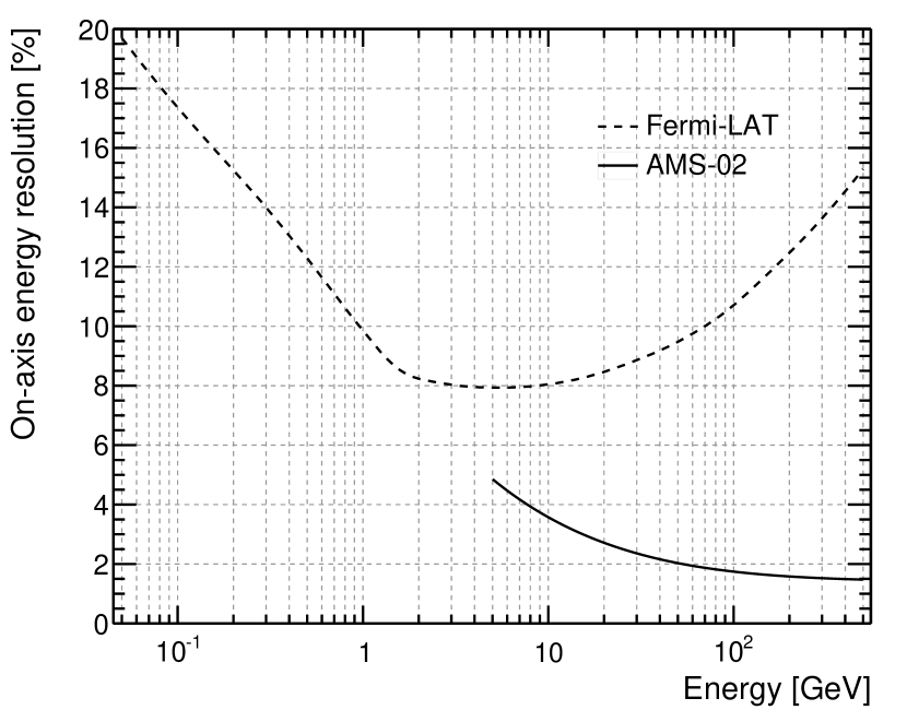
Figure 44: On-axis energy resolution, as a function of the energy, for the Fermi-LAT Ackermann et al. (2012c) and AMS-02 Adloff et al. (2013). AMS-02 features a $17~{}X_{0}$ sampling calorimeter whose energy resolution can be parameterized according to (64) with $a=10.4\%$ and $c=1.4\%$. The Fermi-LAT features a homogeneous calorimeter, $8.6~{}X_{0}$ thick on axis (and a $1.5~{}X_{0}$ tracker converter effectively acting as a pre-shower), and the energy resolution at high energy is dominated by the shower leakage, which can only be partially compensated by using the imaging capabilities of the detector.

VIII.4.2 Hadronic calorimeters

From the standpoint of calorimetry, the main peculiarity of hadronic showers is that some fraction of the energy contained in the non-electromagnetic component does not contribute to the signal (this is what is usually called invisible energy). Endothermic spallation losses are responsible for the vast majority of the invisible energy, as the nuclear binding energy of the released protons, neutrons and heavier aggregates has to be supplied by the shower particles that induce the reactions—and obviously does not contribute to the signal. Furthermore nuclear recoils, neutron captures producing delayed gamma rays, muons and neutrinos, all contribute to the invisible energy.

In addition to that a calorimeter has a different response to the electromagnetic and the non-electromagnetic components of a hadronic shower, in terms of how much of the relative energy is actually translated into visible signal. The ratio of the efficiencies for conversion into detector signal of the two components is customarily referred to as $h/e$, and is characteristic of the material and detector configuration.

As a consequence of these basic facts, typical resolutions for hadronic calorimeters are intrinsically worst than those of the best homogeneous electromagnetic calorimeters (30–40% being a representative figure). It should also be noted that, being the nuclear interaction length typically much larger than the radiation length, hadronic calorimeters need to be (geometrically) thick—and heavy. This is the main reason why hadronic calorimetry, at least in the strict sense the term is used in high-energy physics at accelerators, is not very fashionable in space. One interesting detector concept—used, e.g., in the ATIC Panov et al. (2009) and CREAM Yoon et al. (2011) experiments—is that of exploiting a thick carbon passive target to promote nuclear interaction of the hadrons and then recovering the particle energy by measuring the electromagnetic component of the shower.

VIII.5 Particle identification

There are traditionally four methods for particle identification in high-energy physics: measurement of $dE/dx$, time of flight (TOF) systems, Cherenkov detectors and transition radiation detectors (TRD). In addition to that, modern electromagnetic imaging calorimeters generally provide a high discrimination power for the specific purpose of separating photon- or electron/positron-initiated showers from hadronic showers—so we shall briefly introduce this topic of discussion, too.

Incidentally, all of these techniques are exploited in the AMS-02 experiment operating on the ISS, so the suite of contributions presented by the AMS-02 collaboration at the $33^{th}$ International Cosmic-Ray Conference is potentially a good source of information on the state of the art of particle identification in space. We refer the reader to Lippmann (2012) for a more accelerator-oriented review.

VIII.5.1 Measurement of $dE/dx$

The particle identification is based on the simultaneous measurement of the momentum $p$ and the mean energy loss $dE/dx$ and relies on the fact that the Bethe-Bloch formula is a universal function of $\beta\gamma=p/m$ for all particle species (and therefore it’s different for different masses at the same momentum).

Particle identification systems (e.g. to discriminate protons from pions) based on the mean energy loss have been successfully implemented up to reasonably high energies, well in the relativistic rise (below the saturation point due to the density effect) where typical $dE/dx$ differences are of the order of $10\%$ or so. Since the typical width of the Landau curve for a single sample is generally much larger than this differences, many independent measurements are needed to achieve the required level of accuracy. Typically, due to the long right tail of the Landau curve, some sort of truncated mean is the simplest and most robust estimator of the average energy loss.

In the context of space-based cosmic-ray detectors the $dE/dx$ particle identification technique is customarily used to identify the nuclear species by measuring the atomic number $Z$ through the $Z^{2}$ dependence, as illustrated in figure 45.

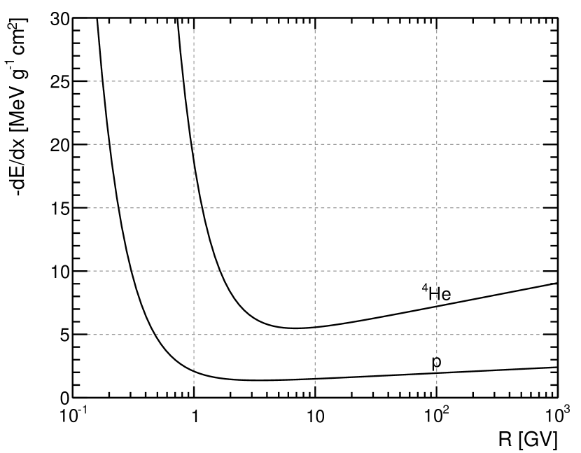
Figure 45: Ionization energy loss, as a function of the rigidity, for protons and He nuclei in silicon. The values are calculated according to (VII.1.1) without any density correction. In real life the separation power of the $dE/dx$ technique is determined by the Landau fluctuations, determining how closely the actual events cluster around the average line.

VIII.5.2 Time of flight

The time of flight method relies on the simultaneous measurement of the particle momentum and velocity through the direct measurement of the time $T$ it takes to the particles to traverse a distance $L$:

$$\beta c=\frac{L}{T}$$ (65)

We can invert the expression $p=m\gamma\beta c$ to obtain the mass of the particle as a function of momentum and velocity:

$$m=\frac{p}{\gamma\beta c}=\frac{p\sqrt{1-\beta^{2}}}{\beta c}=\frac{p}{c}\sqrt{\frac{1}{\beta^{2}}-1}.$$ (66)

By the standard error propagation we get the relative error on the mass measurement:

$$\frac{\sigma_{m}}{m}=\frac{\sigma_{p}}{p}\oplus\gamma^{2}\frac{\sigma_{\beta}}{\beta}.$$ (67)

In practice $L$ is known with a good enough precision that the error on $\beta$ is essentially determined by the time resolution of the system. For $L\sim 1.5$ m and $\sigma_{T}/T\sim 100$ ps (which are somewhat representative of the AMS-02 detector), one can achieve a relative accuracy on the velocity of the order of a few %. Depending on the actual momentum dependence of the momentum resolution and the value of $\gamma$, the mass resolution can be dominated by either one of the two terms.

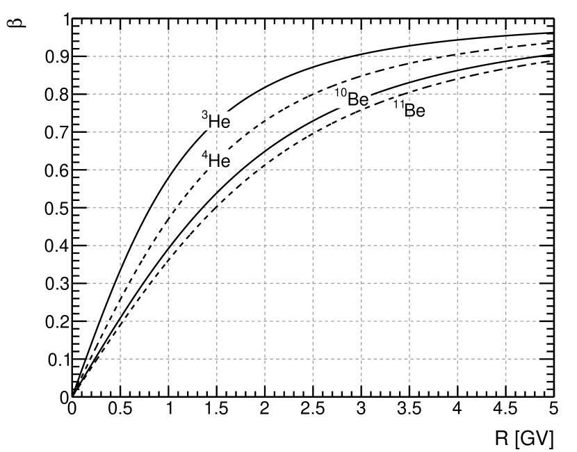
Figure 46: Relation between velocity and rigidity for different isotopes, according to (68).

One practical application of this technique is the measurement of cosmic ray isotopical composition (e.g. the ratio of the differential intensities of ³He/⁴He). This is usually achieved by measuring independently the particle rigidity $R$ with a magnetic spectrometer and its velocity $\beta$ with a TOF system (in addition to the charge $Z$, that can be inferred by means of $dE/dx$ measurements in both the spectrometer and the TOF). In this context (66) is more conveniently written as

$$A=\frac{ZeR\sqrt{1-\beta^{2}}}{m_{p}\beta c^{2}},$$ (68)

where $A$ is the mass number of the nucleus and $m_{p}$ is the mass of the nucleon. Equivalently, for fixed $Z$, the velocity and momentum for nuclei with different mass numbers (i.e., isotopes) will be related to each other by

$$\beta=\left[1+\left(\frac{Am_{p}c^{2}}{ZeR}\right)^{2}\right]^{-\frac{1}{2}},$$ (69)

as illustrated in figure 46 for the two cases of ³He vs. ⁴He and ¹⁰Be vs. ¹¹Be.

In any practical application the finite mass resolution given by (67) will cause events to be distributed around the theoretical line with a finite dispersion—at the level that an event-by-event mass separation could be impossible. Still in these case a template fitting of the data to the separate isotopical mass distribution can in principle allow to recover the composition, at least at intermediate rigidities, where the curves are best separated. We refer the reader to Aguilar et al. (2011) for a detailed description of the light nuclei isotopical composition measurement by the AMS-01 experiment.

VIII.5.3 Cherenkov detectors

As explained in section VII.6, the emission of Cherenkov radiation is a threshold process taking place when a particle moves in a medium with index of refraction $n$ with velocity $\beta>1/n$.

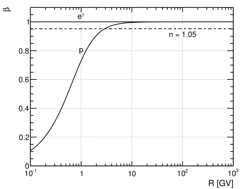
Figure 47: Relativistic $\beta$ factor, as a function of the particle rigidity, for electrons and protons. For illustration purposes, the threshold corresponding to a representative index of refraction $n=1.05$ is shown.

In their simplest form, Cherenkov detectors exploit the existence of this threshold acting as digital counters that allow to distinguish, e.g., electrons and protons over relatively large energy (or rigidity) ranges, as illustrated in figure 47. This was done in many of the early experiments aimed at measuring the positron component of cosmic rays, e.g., in Fanselow (1968); Fanselow et al. (1969); Daugherty et al. (1975); Buffington et al. (1974, 1975). Since $\beta$ approaches $\sim 1$ for $\sim 10$ GV protons, it is difficult to effectively exploit this technique past a few GV.

The steep slope of the intensity of the Cherenkov signal near threshold (see, e.g., figure 39) allows quite an accurate velocity measurement (though in a relatively small window). This can be used to complement TOF system in mass measurements (see VIII.5.2) and, by using a clever arrangement of radiators with different indices of refraction, for actual spectral measurements Obermeier et al. (2011).

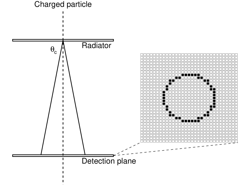
Figure 48: Functional sketch of a ring imaging Cherenkov detector. A cone of Cherenkov radiation produced as the charged particle traverse the radiator is imaged as a ring on the photon detection plane, which provides a measurement of both the intensity of the radiation itself and of the Cherenkov angle $\theta_{c}$.

The most advanced Cherenkov detectors, such as ring-imaging Cherenkov detectors (RICH) exploit all the properties of the Cherenkov effect, including the intensity of the signal and the angular aperture of the light cone (see figure 48 for a simplified, illustrative sketch).

VIII.5.4 Transition radiation detectors

Even a brief summary of the basic considerations going into a practical implementation of a transition radiation detector (see, e.g, Beringer et al. (2012) and Andronic and Wessels (2012)) are beyond the scope of this review. Typically many layers of radiator (i.e., optical interfaces) are needed to achieve a reasonable signal yield, interleaved with suitable radiation detection elements—usually gas detectors. Furthermore, since the transition radiation is emitted in the forward direction at a fairly small angle, it effectively overlaps with the ionization due to the specific energy loss $dE/dx$, and the latter is also an important ingredient of the mix.

As pointed out in section VII.7, a relativistic $\gamma$ factor of the order of $10^{3}$ is needed for the spectrum of the transition radiation to extend in the X-ray domain—i.e., where the emitted photons can be effectively detected on top of the energy deposited by ionization. Figure 49 shows that a relatively large rigidity window—roughly speaking between $\sim 1$ GV and $\sim 1$ TV—exists where the transition radiation can potentially be exploited to discriminate electrons and positrons from protons. (Incidentally, this extends to much higher energies than those accessible to the Cherenkov technique discussed in the previous section).

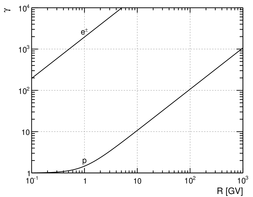
Figure 49: Relativistic $\gamma$ factor, as a function of the particle rigidity, for electrons and protons.

To put things in context, the TRD of the AMS-02 experiment operating on the ISS provides a proton rejection factor (at 90% electron efficiency) in excess of 100 between 1 and 600 GV, peaking around $2\times 10^{4}$ at $\sim 10$ GV Ting (2013).

VIII.5.5 Electron-proton separation in imaging calorimeters

As mentioned in section VII.5, the differences between electromagnetic and hadronic showers are customarily exploited to discriminate high-energy photons, electrons and positrons from hadrons.

As shown in figure 37, for the typical materials used in electromagnetic calorimeters the interaction length $\lambda_{I}$ is 20–30 times larger than the radiation length $X_{0}$ (when expressed in g cm^-2, i.e., normalized to the density). This means that the first interaction is on average at a much larger depth for a hadronic shower than for an electromagnetic one—something like $\sim 20$–30 cm vs. $\sim 1$ cm. Incidentally, since electromagnetic calorimeters are typically thin (less than one $\lambda_{I}$) from the standpoint of hadrons, a significant fraction of high-energy protons just pass through without interacting—i.e., behaving as minimum ionizing particles. (It goes without saying that they are easy to discriminate from photons and electrons.)

In addition to that electromagnetic showers are typically well behaved in that the vast majority of the energy is contained within a few Moliere radii from the shower axis and, fluctuations aside, the shower maximum is located at a predictable position along the axis. In contrast hadronic showers are generally much wider (due to secondaries from inelastic nuclear interactions spreading out with non-negligible transverse momentum) and feature larger fluctuations in both the longitudinal and the transverse development.

IX Instrument Response Functions

In broad terms the instrument response functions (IRF) are specific parameterizations of the instrument performance allowing to convert the count spectra registered by the detector into physically meaningful quantities such as fluxes and spectral indices. In this section we shall try and provide a thorough discussion of the subject, with emphasis on how the response functions tie to the detector design and the basic interaction processes of particles and radiation with the latter. The treatment will be somewhat simplified and aimed at basic sensitivity studies, and the reader is referred, e.g., to Ackermann et al. (2012c) and references therein for a more systematic description of how IRFs are actually used in typical gamma-ray spectral analyses.

IX.1 The role of the event selection

In the context of pretty much any scientific analysis one has to deal with the problem of separating the signal (e.g., the particular CR species under study) from the background (e.g., all the other species, possibly much more abundant, that might mimic, in a way or another, the signal we are interested in). We shall refer to the entire process of isolating the signal from the background as the event selection. While at a fist glance the reader might find awkward to start the discussion about the instrument response functions by bringing up this seemingly unrelated issue, we do so to stress since the beginning that in general the instrument response functions are not intrinsic characteristics of the detector: they always subtend a specific event selection and a detector may very well have different response functions in the context of different analyses. Be wary when you read off a scientific paper or a conference presentation the value of the acceptance for a given instrument quoted as a single plain scalar. Appropriate as it might be for the particular context, keep in mind that there might be hidden energy dependencies and do not forget to double check whether it includes the effect of the selection cuts or not—the difference might be factors to orders of magnitude!

IX.1.1 A different look at cosmic-ray spectra

A comprehensive discussion of the complex (and, to many respects, subtle) issues of event selection and background rejection is outside the scope of this paper. We shall, however, try and put on the table some basic ideas, starting from a somewhat different look on the cosmic-ray spectra—focusing on the ratio between specific differential fluxes, as shown in figure 50.

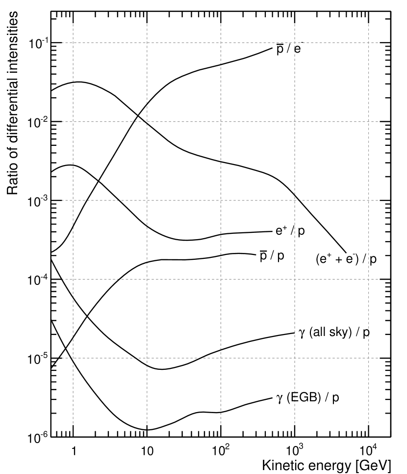
Figure 50: Ratio of the differential fluxes, as a function of the energy, for some specific pairs of cosmic-ray species.

If one is interested in measuring, say, the all-electron $(e^{+}+e^{-})$ spectrum by means of a calorimetric experiment, the main challenge from the standpoint of the background rejection, is the much larger ($10^{2}$–$10^{4}$) proton flux. The all-electron spectrum being significantly steeper ($\Gamma_{e}\sim 3.1$) than the proton spectrum ($\Gamma_{p}\sim 2.75$), the electron-to-proton ratio decreases with energy—and, due to the cutoff measured by H.E.S.S. Aharonian et al. (2008), steepens significantly past $\sim 1$ TeV. This implies that the detector must feature a proton rejection power (see section IX.1.2 for more details) of at least $10^{5}$ in order to have a relatively small background that can be safely subtracted in the data analysis phase. Different how the event topologies for electrons and protons are, this is really saying that we are only allowed to mis-tag one proton in 100,000 (while keeping a reasonable electron efficiency), which is obviously a non trivial task.

Life is even harder for gamma rays, as they are substantially less abundant than any of the four singly-charged CR species. Figure 50 shows that for any celestial gamma ray there are $10^{4}$–$10^{5}$ protons of the same energy. Photons pointing back to their sources, this does not necessarily implies that any gamma-ray analysis is intrinsically more difficult than, say, the measurement of the positron fraction—when studying a gamma-ray source, restricting the sample to a small region of interest around the source itself can allow to reduce the background by orders of magnitude. Nonetheless, the measurement of the faint isotropic extra-galactic gamma-ray background Abdo et al. (2010a) is a good example where a proton rejection factor of the order of $10^{6}$ is really required (and, to this respect, it is fortunate that plastic scintillators can be used to assemble efficient anti-coincidence shields to isolate neutral particles). We should also emphasize that, while much less abundant than protons, high-energy electrons and positrons generally look more similar to photons in calorimetric experiments (they all produce electromagnetic showers), and can therefore constitute an important source of background for gamma rays.

For magnetic spectrometers most of the curves in figure 50 are actually important. At low energy, where charge confusion is negligible, the relevant figures are the $\bar{p}/e^{-}$ ratio for the measurement of the antiproton fraction and $e^{+}/p$ ratio for that of the positron fraction. While achieving a proton/electron rejection power in excess of $10^{4}$ is not really a big issue with modern spectrometers such as AMS-02 or PaMeLa, this was actually a challenge in the early days, when the particle identification capabilities of the instruments were limited—as nicely phrased in Golden et al. (1987): It is the opinion of the investigators that the $e^{+}$ observation is substantially more difficult than the $\bar{p}$ observation […] For negatively charged particles one has to distinguish $\bar{p}$ from a $20$ times higher flux of $e^{-}$ and from atmospheric mesons. In the case of $e^{+}$, however, one must separate the desired particles from protons, which have the same charge and a flux nearly $1000$ times as great. At high energy, on the other hand, where charge confusion is the main limiting factor, the important figures are the $e^{+}/e-$ and $\bar{p}/p$ ratios—and in this regime antiprotons are relatively harder to separate.

In the next section we shall briefly discuss the issue of the background rejection in a slightly more formal fashion. At this point it should be clear, however, that different science analyses, in general, require different levels of rejection power—and hence different event selections and different response functions.

IX.1.2 Discriminating variables and rejection power

The binary problem of separating signal and background in a given event sample is very common in high-energy physics. This is generally achieved by exploiting one or more discriminating variables, i.e. topological properties of the event that are different, on average, for signal and background. The transverse size of the shower in an electromagnetic calorimeter is a prototypical example of a discriminating variables that is useful for separating hadrons from electrons or gamma rays. Other examples include: the signal in a transition radiation detector or in a Cherenkov counter, the average $dE/dx$ in the layers of a tracking detectors, the pulse height in a scintillator and many others. When a high level of purity is required, it is customary to use many different variables, possibly combining them by means of multivariate classification techniques such as Fisher discriminants, classification trees, boosted decision trees and others.

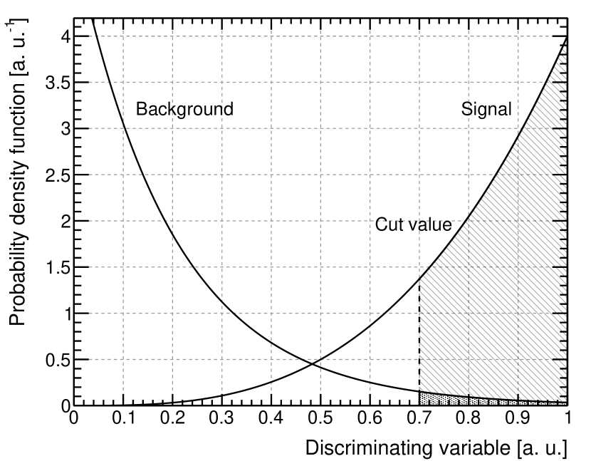
Figure 51: Illustrative probability density functions, for signal and background, of a generic discriminating variable (note that the shape of the curves, though not necessarily irrealistic, is purely fictional).

Figure 51 shows an example of the probability density functions, for signal and background, of a fictional discriminating variable $x$ in the interval $[0,1]$ that we shall use for illustrative purposes. A cut on the discriminating variable (e.g., the act of selecting events for which, say, $x>x_{0}$) defines the values of the efficiency for signal and background:

$$\varepsilon_{\rm sig} =\int_{x_{0}}^{1}p_{\rm sig}(x)dx$$

$$\varepsilon_{\rm bkg} =\int_{x_{0}}^{1}p_{\rm bkg}(x)dx.$$ (70)

(At this point you want to be sure that $\varepsilon_{\rm sig}>\varepsilon_{\rm bkg}$, and possibly $\varepsilon_{\rm sig}\gg\varepsilon_{\rm bkg}$; otherwise you should probably look for a better discriminating variable.)

Given a selection cut (or a set of selection cuts), the rejection power $\mathcal{R}$ is formally defined as

$$\mathcal{R}=\frac{\varepsilon_{\rm sig}}{\varepsilon_{\rm bkg}}.$$ (71)

The rejection power is a useful concept as it relates the number of signal and background events before and after the cut

$$\left.\frac{n_{\rm sig}}{n_{\rm bkg}}\right|_{\rm after}=\mathcal{R}\left.\frac{n_{\rm sig}}{n_{\rm bkg}}\right|_{\rm before}.$$ (72)

In order to be able to do a meaningful background subtraction, one typically wants the number of signal events to be much larger than the number of background events in the final sample, which sets the necessary rejection power necessary for a given analysis, once the initial ratio is known (again, see figure 50). It is worth stressing that whether it is practically possible to achieve the necessary rejection power is hostage of the shape of the probability density functions of the discriminating variables. In real life the optimal cut value is determined by a trade off between the signal efficiency and the rejection power, as illustrated in figure 52.

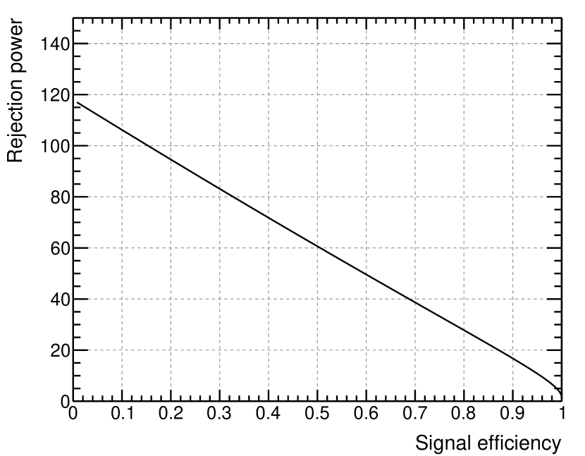
Figure 52: Illustrative trade-off between the signal efficiency and the rejection power. The plot refer to the probability density functions shown in figure 51.

IX.2 Effective Area, Acceptance and Field of View

Fluxes from (gamma-ray) point sources are customarily measured in particles per unit area, time and energy, e.g. in ${\rm m}^{-2}~{}{\rm s}^{-1}~{}{\rm GeV}^{-1}$. When dealing with a (at least approximately) isotropic flux of charged particles or photons, the intensity of such flux is more conveniently measured in particles per unit area, time, energy and solid angle, e.g. in ${\rm m}^{-2}~{}{\rm s}^{-1}~{}{\rm GeV}^{-1}~{}{\rm sr}^{-1}$. In the first case the conversion factor between the differential source flux $dF/dE$ and the differential count spectrum $dN/dE$ measured by the detector (in s^-1 GeV^-1) is the effective area $A_{\rm eff}$:

$$\frac{dN}{dE}=A_{\rm eff}\times\frac{dF}{dE}.$$ (73)

(Strictly speaking, as we shall see in the following, this is true only if the effects of the energy dispersion and the point-spread function are negligible.) In the latter case the conversion factor between the differential intensity $dJ/dE$ and the differential count spectrum $dN/dE$ measured by the detector (again, in s^-1 GeV^-1) is the acceptance $G$:

$$\frac{dN}{dE}=G\times\frac{dJ}{dE}.$$ (74)

It goes without saying that the effective area is measured in m² and the acceptance in m² sr.

Equations (73) and (74) are effectively operative definitions of the effective area and acceptance. For the reason stated above, the concept of effective area is seldom used by the cosmic-ray community; on the other hand the acceptance (call it with any of the different names mentioned in the previous paragraph) is relevant for both cosmic-ray and gamma-ray detectors. We also note, in passing, that typically we use the equations (73) and (74) in the other direction, i.e., we divide the measured count spectrum by the effective area or acceptance to recover the actual flux or intensity. We shall see that, when the energy redistribution due to the finite detector energy resolution is not negligible, this has profound implications.

The effective area is in general defined for a give energy $E$ and viewing direction. In the following of this section we shall indicate with $\theta$ and $\phi$ the polar and azimuthal angles in instrument coordinates. In broad terms (and in a somewhat arbitrary fashion), the effective area can be factored out in three different pieces:

$$A_{\rm eff}(E,\theta,\phi)=A_{\rm geo}(\theta,\phi)\varepsilon_{\rm det}(E,\theta,\phi)\varepsilon_{\rm sel}(E,\theta,\phi),$$ (75)

where the $A_{\rm geo}(\theta,\phi)$ is the geometric cross-sectional area presented by the instrument toward a given direction, $\varepsilon_{\rm det}(E,\theta,\phi)$ is the detection efficiency at a given energy and incidence direction (for gamma-ray detectors this includes the conversion efficiency) and $\varepsilon_{\rm sel}(E,\theta,\phi)$ is the efficiency of the selection cuts (e.g., for suppressing the backgrounds). The last factor in equation (75) makes it clear that the effective area, as we said, is not an intrinsic property of the detector, as it subtends a specific event selection.

The effective area at normal incidence (or on-axis effective area) will be used frequently in the following and deserves a dedicated notation

$$A_{\rm eff}^{\perp}(E)=A_{\rm eff}(E,\theta=0).$$ (76)

(Note that, for $\theta=0$, there is a degeneracy on $\phi$ and $A_{\rm eff}$ only depends on $E$.)

The acceptance (or geometric factor) is formally defined as the integral of the effective area over the solid angle:

$$G(E)=\int_{\Omega}A_{\rm eff}(E,\theta,\phi)d\Omega,$$ (77)

and the field of view as the ratio between the geometric factor and the effective area at normal incidence:

$${\rm Fo\kern-1.0ptV}(E)=\frac{G(E)}{A_{\rm eff}^{\perp}(E)}=\frac{\int_{\Omega}A_{\rm eff}(E,\theta,\phi)d\Omega}{A_{\rm eff}^{\perp}(E)}.$$ (78)

(Note that when the angular dependence of the effective area is different at different energies, the field of view does depend on energy, see, e.g., Ackermann et al. (2012c).)

IX.2.1 The Ideal Planar Detector

In this section we shall consider the (somewhat irrealistic) scenario of a planar (i.e. infinitely thin) detector with side $l$. We shall assume that our detector is sensitive to all the particles coming from the upper hemisphere and crossing it, irrespectively of the event energy. Sure enough most of the actual detectors do not quite look like this, but as we shall see this academic example allows to discuss the basic concepts introduced in the previous section in a simple context.

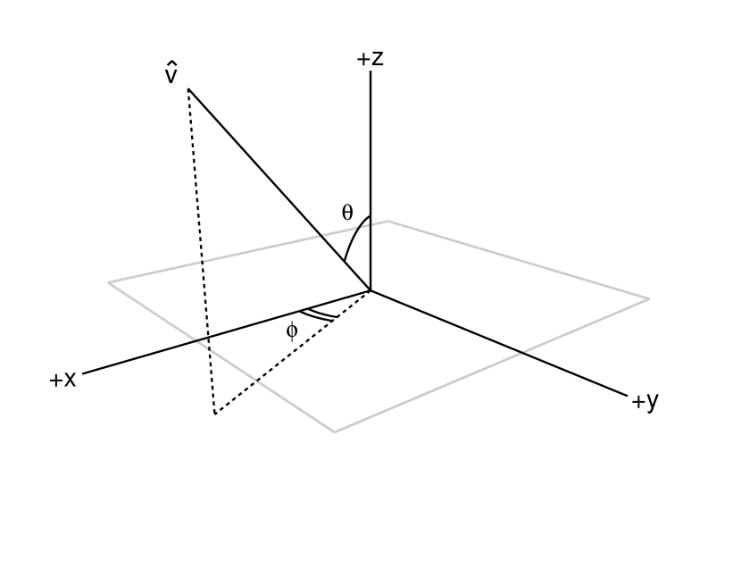
Figure 53: Sketch of an ideal planar detector. The $\theta$ and $\phi$ angles define the basic reference system (in instrument coordinates) used throughout this section to parameterize the instrument response.

In this case the effective area at normal incidence is simply the geometrical area of the detector $S=l^{2}$. It is clear that $A_{\rm eff}$ only depends on the polar angle $\theta$:

$$A_{\rm eff}(E,\theta,\phi)=S\cos\theta,$$ (79)

and the acceptance reads:

$$G=S\int_{0}^{2\pi}\!d\phi\int_{0}^{\pi}\!\cos\theta\sin\theta d\theta=\pi S.$$ (80)

The field of view, finally, is

$${\rm Fo\kern-1.0ptV}=\frac{G}{S}=\pi.$$ (81)

The reader might be wondering why the field of view is not $2\pi$—after all our detector sees the entire upper hemisphere, doesn’t it? Well, that would be if the effective area was independent of the off-axis angle. In our case the effective area is monotonically decreasing with $\theta$, and in fact it is zero at $\theta=90^{\circ}$. This is the basic reason why the field of view is half the value one might naïvely expect. In turn, this points out that the field of view is not the solid angle subtended by the maximum off-axis angle the detector is accepting events from. More on that in the next section.

IX.2.2 A more realistic example

Figure 54 shows a more realistic (though still fictional) example of cosmic-ray detectors. We have seen the sketches of some actual detectors back in figure 12.

Figure 54: Sketch of a simple, semi-realistic detector. The $\theta$ and $\phi$ angles define the basic reference system (in instrument coordinates) used throughout this section to parameterize the instrument response.

The basic detector layout and the arrangement of its active elements determines the maximum off-axis angle $\theta_{\rm max}$ at which events can be recorded (note that $\theta_{\rm max}$ can possibly depend on the event energy, e.g., if a longer path length in the calorimeter is required for reconstructing high-energy events, but we shall neglect this possible dependence for the sake of simplicity—and we shall also assume that the selection cuts do not introduce any energy dependence). This is in general not enough to estimate the actual field of view, as one really needs a full parameterization of the $\theta$-dependence of the effective area. The crudest possible approximation that one can do is to assume that the effective area for any given theta, relative to the on-axis effective area, decreases linearly with $\cos\theta$, with the proper boundary conditions

$$A_{\rm eff}(\theta)=A_{\rm eff}^{\perp}\left(\frac{\cos\theta-\cos\theta_{\rm max}}{1-\cos\theta_{\rm max}}\right),$$ (82)

as shown in figure 55.

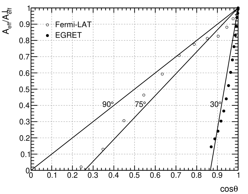
Figure 55: Graphical representation of our crude model (82) for three illustrative values of $\theta_{\rm max}$: $90^{\circ}$ (the planar detector), $75^{\circ}$ and $30^{\circ}$. Overlaid are the actual values for the Fermi-LAT and EGRET, which are reasonably represented (within $15\%$ or so) by the $75^{\circ}$ and $30^{\circ}$ models, respectively.

While the author would not recommend counting on this kind of models for an actual science analysis, equation (82) is typically adequate for back-of-the-envelope calculations. We note, in passing, that the planar detector discussed in the previous section is a particular case (with $\theta_{\rm max}=90^{\circ}$) of this general family of effective area curves.

The acceptance for our naïve detector model reads

$$G=\int_{0}^{2\pi}\!\!\!\!d\phi\int_{0}^{\theta_{\rm max}}\!\!\!\!\!\!\!\!A_{\rm eff}(\theta)\sin\theta d\theta=\pi A_{\rm eff}^{\perp}(1-\cos\theta_{\rm max})$$ (83)

(you can explicitly calculate the integral or just look at figure 55: when you note that $\sin\theta d\theta=-d\cos\theta$ we are really trying to calculate the area of a triangle).

The field of view is then easily calculated as:

$${\rm Fo\kern-1.0ptV}=\pi(1-\cos\theta_{\rm max}),$$ (84)

which reduces to the results we obtained for the planar detector when $\theta_{\rm max}=90^{\circ}$. We note that, as in the case of the planar detector, this is exactly half of the solid angle subtended by the cone defined by $\theta_{\rm max}$.

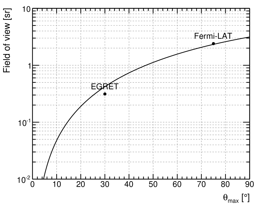
Figure 56: Field of view as a function of $\theta_{\rm max}$, as estimated from equation 84. Overlaid are the actual values for the Fermi-LAT and EGRET.

IX.2.3 Event distributions in instrument coordinates

It is interesting to consider the probability density function of the event directions in instrument coordinates—most notably that of the off-axis angle $\theta$—for an isotropic input distribution. Looking at equation (82) and figure 55 one might be tempted to conclude that $dN/d\theta$ has its maximum for $\theta=0$, which is not quite true. Figure 55 represents $dN/d\cos\theta$, while

$$\frac{dN}{d\theta}=\frac{dN}{d\cos\theta}\left|\frac{d\cos\theta}{d\theta}\right|=\frac{dN}{d\cos\theta}\sin\theta.$$ (85)

One can easily recognize the solid angle term in the last piece.

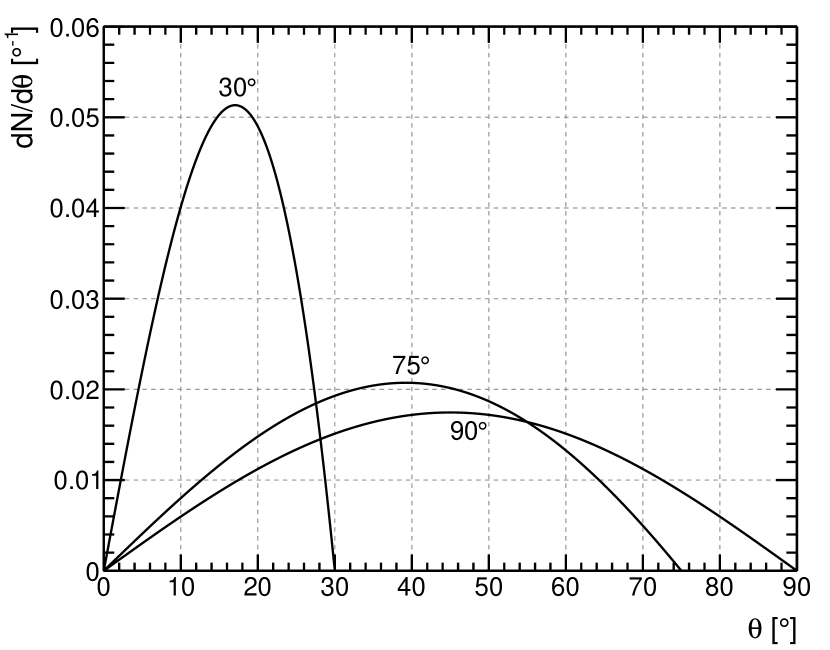
Figure 57: Illustrative $\theta$ distributions, taken from equation 86.

It is easy to calculate the normalized probability density function

$$\frac{dN}{d\theta}=\frac{(\cos\theta-\cos\theta_{\rm max})\sin\theta}{(\frac{1}{2}+\frac{1}{2}\cos^{2}\theta_{\rm max}-\cos\theta_{\rm max})}.$$ (86)

In the limit in which our naïve model is a reasonable approximation of reality, this is actually a very useful relation, as it allows to derive a series of metrics germane to the path length of the events in the detector. For one thing one could calculate the average value or the most probable value of $\theta$—this is not too difficult, though somewhat lengthy. Since the path length in the detector at a given incidence angle is given by $1/\cos\theta$, the most important figure of merit is the expectation value of this quantity, which physically corresponds to the average amount of material $\left<t\right>$ traversed by an event, relative to the instrument depth on axis $t_{0}$:

$$\frac{\left<t\right>}{t_{0}}=\int_{0}^{\theta_{\rm max}}\frac{dN}{d\theta}\frac{1}{\cos\theta}d\theta.$$ (87)

The integral is not as difficult as it might seem at first glance and the answer is:

$$\frac{\left<t\right>}{t_{0}}=\frac{1+\cos\theta_{\rm max}(\ln\left|\cos\theta_{\rm max}\right|-1)}{(\frac{1}{2}+\frac{1}{2}\cos^{2}\theta_{\rm max}-\cos\theta_{\rm max})}.$$ (88)

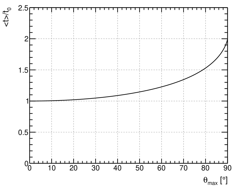
Figure 58: Average path length (relative to the depth at normal incidence) for an isotropic input distribution as a function of the maximum off-axis angle $\theta_{\rm max}$.

This is plotted in figure 58, which makes clear that the effect can be quite noticeable for instruments with a large field of view. To put things in context, for the Fermi-LAT, with a total depth at normal incidence of $10.1~{}X_{0}$ and a maximum off-axis angle of $\theta_{\rm max}\sim 75^{\circ}$, equation (88) gives an average path-length of $\left<t\right>\sim 14~{}X_{0}$. As one can imagine, this has rather important implications for the energy reconstruction at high energy.

IX.3 Energy Dispersion

The energy dispersion $D_{E}(E;E_{\rm true})$ is the probability density to measure an energy $E$ for an event with (true) energy $E_{\rm true}$. In general the energy dispersion depends on the incidence direction and impact point of the incoming particle, but in the following of the section we shall pretend this is not the case. Unlike the effective area, the energy dispersion is not a scalar, but a probability density function. From an operational standpoint, the energy dispersion is essentially the distribution of the measured energy values for a monochromatic particle beam. It goes without saying that the energy dispersion is in general different for different cosmic-ray species—most notably it is typically much narrower and well-behaved for electrons, positrons and photons than for hadrons.

The energy resolution $\sigma_{E}/E$ is typically defined as the half width of the smallest energy window containing 68% of the energy dispersion, divided by the most probable value of the energy dispersion itself. Difficult as it might seem, this definition reduces to the ratio $\sigma/\mu$ in the gaussian case. At any given energy the energy resolution is a scalar and it is the figure of merit which is customarily used to summarize the information contained in the energy dispersion.

IX.3.1 Effect of a finite energy resolution

When measuring particle spectra binned in energy, the energy dispersion originates the phenomenon of the event migration, or bin-to-bin migration—namely the fact that events that would really belong to a given energy bin are assigned to a different (hopefully neighbor) bin. Strictly speaking, this implies that our operational definitions of the effective area and acceptance, equations (73) and (74), no longer hold: one cannot divide the count spectrum by the effective area or the acceptance to recover the actual source flux or intensity. Whether the effect is negligible or not really depends on the measurement setup, i.e., the details of the energy dispersion and the input spectrum. The effect is sketched in figure 59.

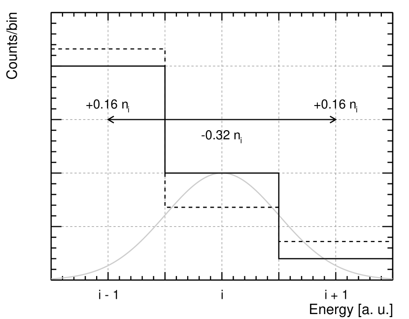
Figure 59: Graphical illustration of the energy redistribution, or bin-to-bin migration. In this case the bin width is equal to the energy resolution and the gray gaussian illustrates the energy dispersion at the center of the $i$-th bin.

We note that, when measuring steeply falling spectra such as the typical cosmic-ray spectra, a prominent right tail in the energy dispersion is potentially more dangerous than a long left tail, as even a fractionally small spillover from a low-energy bin can be significant in the next energy bins, where the number of counts is much smaller.

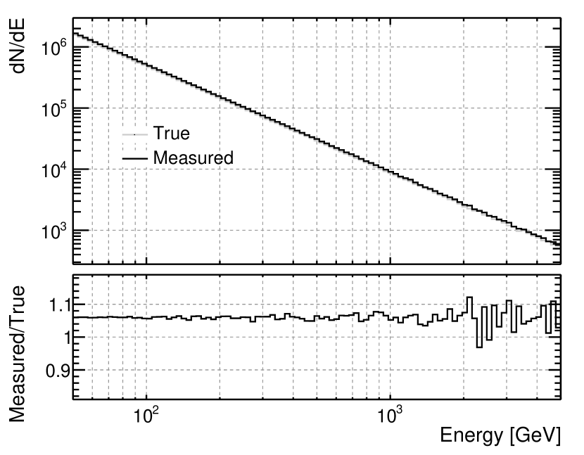
Figure 60: Toy Monte Carlo simulation of an energy spectrum proportional to $E^{-2.75}$, measured with an energy resolution of 30% (constant in energy and with a gaussian energy dispersion). The setup is largely simplistic, but not totally unreasonable as an illustration of a typical measurement of the primary CR proton spectrum. The net effect, of the order of $\sim 6\%$, is something that must be taken into account for systematic-limited measurements.

Interestingly enough, a constant energy resolution $\sigma_{E}/E$ (i.e., an energy dispersion whose width increases linearly with the energy), when convoluted with a power-law count spectrum with index $\Gamma$, causes an offset constant in energy, as illustrated with a toy Monte Carlo simulation in figure 60. Formally, the convolution is written as

$$\frac{dN}{dE}= \int_{-\infty}^{\infty}\frac{dN}{d\epsilon}D_{E}(E;\epsilon)\;d\epsilon=\int_{-\infty}^{\infty}\!\!\!\!N_{0}\epsilon^{-\Gamma}D_{E}(E;\epsilon)\;d\epsilon$$

and, while this can be quite complicated to solve in the general case, there is a few things than can be inferred in a model-independent fashion. As the normalization factor of the energy dispersion is inversely proportional to the energy resolution (the normalization factor being, e.g., $1/\sqrt{2\pi}$ in the gaussian case), we can rewrite the convolution

$$\frac{dN}{dE}= \int_{-\infty}^{\infty}\frac{N_{0}}{(\sigma_{E}/E)\epsilon}\epsilon^{-\Gamma}w(E;\epsilon)\;d\epsilon=$$

$$\frac{N_{0}}{(\sigma_{E}/E)}\int_{-\infty}^{\infty}\epsilon^{-(\Gamma+1)}w(E;\epsilon)\;d\epsilon,$$

where $w(E;\epsilon)$ is a window function which is equal to $1$ for $E=\epsilon$ and effectively limits the integral to a region $\sim 2k\sigma_{E}$ wide around $E$, $k$ being a numerical factor of the order of $1$. If we let $s=k\sigma_{E}/E$, we can rewrite the convolution as

$$\frac{dN}{dE}\propto \frac{N_{0}}{(\sigma_{E}/E)}\int_{E(1-s)}^{E(1+s)}\epsilon^{-(\Gamma+1)}\;d\epsilon=$$

$$\frac{N_{0}E^{-\Gamma}}{(\sigma_{E}/E)\Gamma}\left[(1-s)^{-\Gamma}-(1+s)^{-\Gamma}\right]$$

The ratio $r$ between the count spectra in measured and true energy can be written as

$$r\propto\frac{1}{(\sigma_{E}/E)\Gamma}\left[(1-s)^{-\Gamma}-(1+s)^{-\Gamma}\right]$$

(note that the dependence on $E$, as anticipated, disappeared). Now, the expression in square brackets can be expanded—and you need to go all the way up to the third order if you want to get the first non-vanishing correction—giving

$$r-1\approx\frac{k^{2}(\Gamma-1)(\Gamma-2)}{3}\left(\frac{\sigma_{E}}{E}\right)^{2},$$

which contains the relevant dependencies on $\Gamma$ and $\sigma_{E}/E$. Particularly, we note that the offset scales with the square of the energy resolution and that it is identically $0$ for $\Gamma=2$ (interestingly enough, this is a typical spectral index for gamma-ray sources). We also note that the offset is always positive for $\Gamma>2$, which has to do with the fact that, with a steep enough spectrum, the effect of the right tail of the energy dispersion dominates over that of the left tail.

It it actually easy to explicitly work out the calculation for the (admittedly, purely academic) example of a uniform energy dispersion and the solution turns out to be

$$r-1\approx\frac{(\Gamma-1)(\Gamma-2)}{2}\left(\frac{\sigma_{E}}{E}\right)^{2}.$$ (89)

Since this formula actually works for the much more relevant case of a gaussian energy dispersion, it can be quite useful in practice. For $\Gamma=2.75$ and $\sigma_{E}/E=30\%$, equation (89) gives a value of $r-1=5.9\%$, in agreement with the toy Monte Carlo in figure 60. The general behavior of equation (89) is illustrated in figure 61.

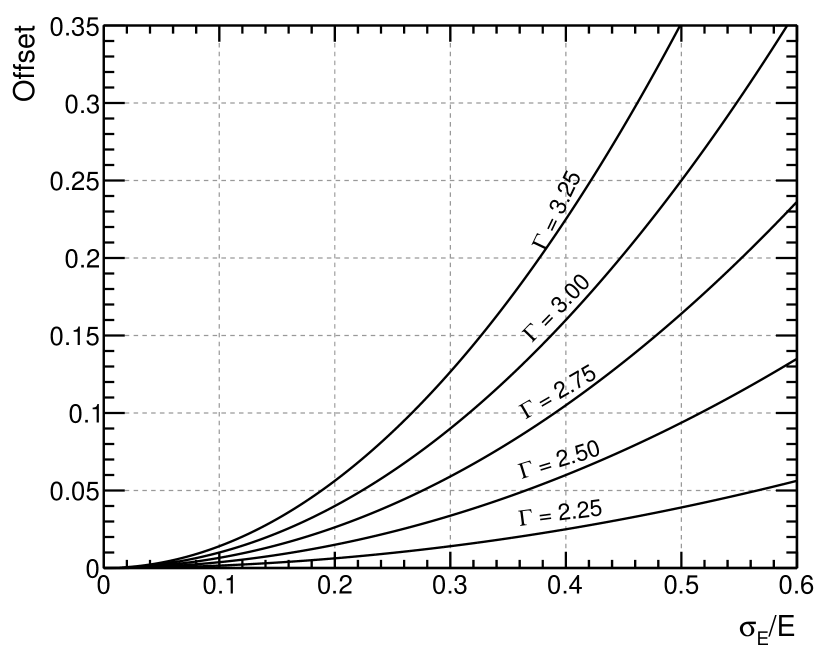
Figure 61: Offset caused by a finite energy resolution $\sigma_{E}/E$, coupled to a power-law count spectrum with index $\Gamma$, for different values of $\Gamma$, according to equation (89).

We conclude noting that, when coupling an energy-dependent acceptance to the (energy dependent) energy dispersion, one can potentially get all kinds of spectral distortion even in the case of a plain power-law input spectrum. In general the problem must really be studied on a case-by-case basis and the reader is referred to Ackermann et al. (2012c) for more details.

IX.3.2 The absolute energy scale

The uncertainty in the absolute energy scale (i.e. in the most probable value of the energy dispersion) is another source of potential spectral deformation. Verifying the absolute energy scale in orbit is a non trivial task, as there isn’t very many spectral features (at know position) available—see however section XI.2.3 for more details. The energy scale is typically calibrated on the ground with particle beams up to the highest available beam energies, but then extrapolating the response at (possibly much) higher energies is a challenge in many contexts.

It is easy enough to show that, in the case of power-law count spectrum and a constant fractional error $s_{E}$ on the energy scale—e.g., the measured energy is systematically higher or lower than the true energy by a factor $(1+s_{E})$ on average—the net effect is again a fractional offset constant in energy, similar to that induced by a finite energy resolution. In this case the ratio $r$ between the count spectra $dN/dE$ in measured and true energy is given by the combination of two effects: the numerator $dN$ increases (or decreases, if $s_{E}$ is negative) by a factor $(1+s_{E})^{\Gamma}$, and the denominator increases (or decreases) by a factor $(1+s_{E})$:

$$r=\frac{(1+s_{E})^{\Gamma}}{(1+s_{E})\phantom{{}^{\Gamma}}}=(1+s_{E})^{\Gamma-1}\approx 1+(\Gamma-1)s_{E},$$

or

$$r-1\approx(\Gamma-1)s_{E}.$$ (90)

For $\Gamma=3$, for instance, an error of the absolute energy scale of 5% implies a corresponding error on the flux measurement of 10%. As for the case of a finite energy resolution discussed in the previous section, we conclude noting that an energy-dependent error on the absolute energy scale (or a constant error coupled to a curved input spectrum) do cause spectral deformations that need to be studied case by case.

IX.3.3 Correcting for the energy dispersion

As mentioned in passing before, if the effect of the energy dispersion cannot be ignored, equations (73) and (74) cannot be used, as they relate the source flux to the observed counts—through the effective area or the acceptance—all evaluated at the true event energy. In general, events with true energy $E$ will contribute instead to the counts measured at a different energy $E^{\prime}$ due to the energy redistribution. If we are doing a binned analysis, the count rate in the $i$-th (measured) energy bin will be a sum of contributions from the source flux in several (true) energy bins:

$$n_{i}=C_{ij}F_{j}.$$ (91)

$C_{ij}$ is customarily called the detector response matrix (DRM). If $n_{i}$ is measured in s^-1, or counts per second, and $F_{j}$ in m^-2 s^-1, the detector response matrix has the physical dimensions of an area—and it is in fact a generalization of the effective area. If the detector response matrix is diagonal, we are effectively back to the original discussion.

It goes without saying that one is typically interested in using equation (91) in the opposite direction, i.e., to recover the actual source flux from the measured counts. The reader might be tempted to say that the problem is trivially invertible by doing

$$F_{i}=\left(C_{ij}\right)^{-1}n_{j}.$$ (92)

An effective way to understand that this is actually a terrible idea is a simple and amusing argument by Barlow Barlow (2000). Assume that we have two energy bins and the detector response matrix reads, in some units:

$$C=\begin{pmatrix}0.6&0.4\\ 0.4&0.6\end{pmatrix}.$$

The reader can verify directly that the inverse matrix reads

$$C^{-1}=\begin{pmatrix}\phantom{-}3&-2\\ -2&\phantom{-}3\end{pmatrix}.$$

If we measure $n=(10,10)$, equation (92) gives a flux estimate of $F=(10,10)$—fair enough. But if we do measure $(13,7)$, which is within a mild statistical fluctuation from the previous pair, we get $(25,-5)$, i.e. a nonsense. In some sense the answer is right: $(25,-5)$, folded with our DRM, gives indeed $(13,7)$. But it’s an answer with little or no physical meaning.

As it turns out, unfolding is a thoughtfully studied problem and algorithms exist that can do a decent job under many different conditions. If one is only interested in fitting a spectral model to a series of data point, the forward folding approach is typically superior.

IX.4 Rigidity Resolution

We have worked out the basic formalism of the rigidity measurement by a magnetic spectrometer in section VIII.2. In this section we shall study the problem in some more details.

At low rigidity the track deflection is large and the the multiple scattering is the dominant contribution to the rigidity resolution. As both the multiple scattering angle (40) and the bending angle (60) scale as $1/R$, the multiple scattering term in the rigidity resolution is a constant (i.e., does not depend on $R$), at least as long as $\beta\approx 1$:

$$\frac{\sigma_{R}^{\rm MS}}{R}=\frac{\theta_{\rm MS}^{\rm plane}}{\theta_{\rm B}}\sim\frac{0.0136\sqrt{t}(1+0.038\ln t)}{0.3~{}\beta~{}B~{}[{\rm T}]~{}L~{}[{\rm m}]}.$$ (93)

At high energy, in contrast, assuming that $L$ and $B$ are known with enough precision, the momentum resolution is determined by the hit resolution $\sigma_{\rm hit}$ of the tracking detectors:

$$\frac{\sigma_{R}^{\rm hit}}{R}=\frac{\sigma_{s}}{s}\sim\frac{8R\sigma_{\rm hit}}{eBL^{2}}=\frac{R~{}[{\rm GV}]~{}\sigma_{\rm hit}~{}[{\rm mm}]}{37.5~{}B~{}[{\rm T}]~{}L^{2}~{}[{\rm m^{2}}~{}]},$$ (94)

and, as we anticipated in section VIII.2, degrades linearly with the rigidity:

$$\frac{\sigma_{R}}{R}=\frac{\sigma_{s}}{s}\propto R.$$ (95)

It should be emphasized that we are deliberately overlooking the fact that a magnetic spectrometer has typically several tracking and the information from the position sensitive detectors is combined through some sort of pattern recognition and track fitting algorithm. There are many more subtleties involved, such as the fact that the hit resolution is different for different particle types (e.g., for protons and alpha particles), but we’ll just move on, as we’re just interested in the orders of magnitude.

We can finally sum the two contributions in quadrature to get an expression for the rigidity resolution as a function of the rigidity:

$$\frac{\sigma_{R}}{R}=\frac{\sigma_{R}^{\rm MS}}{R}\oplus\frac{\sigma_{R}^{\rm hit}}{R}.$$ (96)

As already mentioned, the multiple scattering term dominates at low energy, while the detector resolution term, increasing linearly with $R$ dominates at high energy.

IX.4.1 The Maximum Detectable Rigidity

The maximum detectable rigidity (MDR) is formally defined as the value of the rigidity for which the rigidity (or momentum) resolution is $1$ (i.e., $100\%$). As we shall see in a second, the MDR sets the upper bound of rigidity measurable by a given setup. Posing the right-hand side of equation (94) equal to $1$ gives an easy expression to work with:

$${\rm MDR}=\frac{37.5~{}B~{}[{\rm T}]~{}L^{2}~{}[{\rm m^{2}}]}{\sigma_{\rm hit}~{}[{\rm mm}]}.$$ (97)

With all the caveats mentioned in the previous section, if we plug in the relevant figures for the PaMeLa magnetic spectrometer ($B=0.43$ T, $L=0.445$ m, $\sigma_{\rm hit}\approx 3~{}\mu$m) we end up with a MDR of $1.05$ TV, which is close enough to the actual value of $1.2$ TV predicted by a full Monte Carlo simulation and measured on orbit.

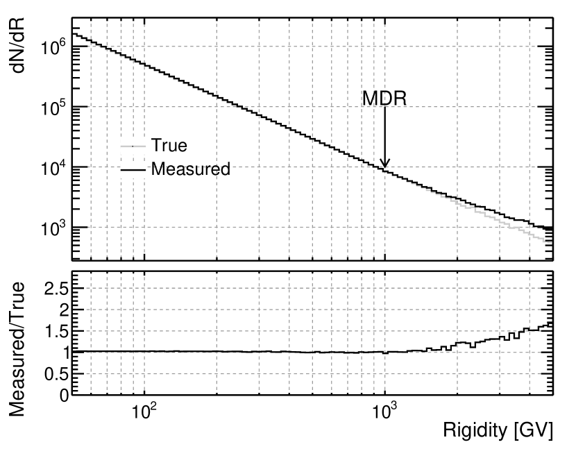
Figure 62: Effect of a finite rigidity resolution on a toy Monte Carlo power-law spectrum with index $2.75$, mimicking the primary cosmic-ray proton spectrum, for a maximum detectable rigidity of $1$ TV. (For completeness, the smearing used for this illustration is gaussian in $1/R$. Though the relative fluctuation in $R$ and $1/R$ are the same, the result would have been somewhat different if the smear was done in the rigidity space—we stress, however, that the point of the exercise was not to develop a realistic model of the rigidity dispersion.)

The effect of the finite rigidity resolution on a typical CR spectrum is illustrated with a toy Monte Carlo in figure 62. For rigidity values above the MDR the spectral distortions can be very noticeable. This is germane to the discussion about the effect of the energy dispersion in section IX.3.3, with the noticeable difference that when approaching the MDR correcting for the redistribution becomes quickly difficult.

It should be also stressed that, while we presented the MDR as an intrinsic characteristic of the detector, it is really an event-by-event quantity. As the magnetic field is not exactly uniform in the detector and the deflection is best measured for tracks with more hits, the quality of momentum reconstruction is in general different for events with the same rigidity impinging in different points of the detector and/or from different directions. In any real science analysis this is all properly taken into account (e.g., it is customary to select events based on their MDR).

IX.4.2 Charge confusion

The rigidity resolution worsening at high rigidity is not the end of the story. As tracks get more and more straight with increased rigidity, the charge confusion (namely the fact that a track with positive curvature can be reconstructed with negative curvature) comes into play. The charge confusion is a combined effect with contributions from the spillover (i.e., errors in the sign determination due to the finite hit resolution of the tracking detectors) and a series of (particle-dependent) effects such as the production of delta rays and bremsstrahlung photons from the primary particle and spurious hits from either electronic noise or backsplash.

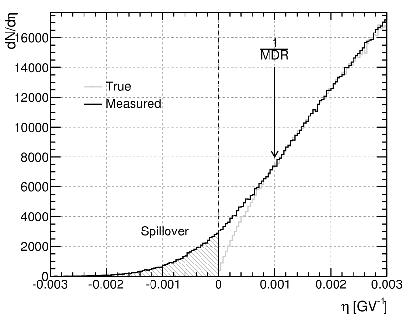
Figure 63: Illustration of the spillover effect. Here the same (true and measured) spectra in figure 62 are shown in the $\eta$ space. We remind again that for this toy simulation the smearing is gaussian in $\eta$, assuming a MDR of $1$ TV.

The spillover, is better studied with the change of variable

$$\eta=\frac{1}{R}$$ (98)

As $R$ tends to infinity, $\eta$ tends to zero (even more importantly, keeping its sign). As shown in figure 63 the effect becomes noticeable as the particle rigidity approaches the MDR. While this might be irrelevant for the more abundant species, the spillover can be the limiting factor for rare species (e.g., cosmic-ray protons are so much more abundant than antiprotons that any $\bar{p}$ spillover has virtually no effect, but the opposite is clearly not true).

IX.4.3 A case study: the AMS-02 rigidity resolution

The AMS-02 magnetic spectrometer, in the permanent magnet configuration currently operating on the ISS, includes an inner tracker (with 7 layers of double-sided silicon-strip detectors) immersed in the magnetic field and two additional layers (that we shall refer to as L1 and L9) aimed at increasing the lever arm (and therefore the MDR). A sketch of the apparatus is shown in figure 12. Table 9 summarizes the basic figures that enter into modeling the rigidity resolution of the detector.

Quantity	Value
Hit resolution ($\sigma_{\rm hit}$)	$10~{}\mu$m
Overall tracker thickness ($t_{\rm TKR}$)	$0.5~{}X_{0}$
Height of the inner tracker ($L_{\rm inner}$)	$0.82$ m
Total tracker height ($L_{\rm TKR}$)	$2.95$ m
Magnet height ($L$)	$1.1$ m
Magnetic field ($B$)	$0.14$ T

Table 9: Basic characteristics of the AMS-02 magnetic spectrometer determining the rigidity resolution of the instrument (from Ting (2013)). The total tracker thickness has been divided by the number of layers (9) to be plugged in equation (96).

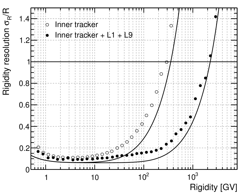
Figure 64: Naïve model of the proton rigidity resolution for the AMS-02 spectrometer (lines), compared with the prediction of the full Monte Carlo detector simulation Ambrosi and et al. (2013a). Our simple formula (96) is able to reproduce the general shape (including the raise below $\sim 1$ GeV due to the $\beta$ term in the multiple scattering formula) and predicts a MDR of $350$ GV and $2.3$ TV for the two configurations, to be compared with $250$ GV and $2$ TV reported in Ambrosi and et al. (2013a).

For the inner tracker, the numbers can be plugged directly into equation (96) to get a rough estimate of the rigidity resolution as a function of rigidity. To first order the bending power for the inner tracker $BL_{\rm inner}^{2}$ can be scaled to the full tracker, including L1 and L9, by multiplying for the factor

$$f=\frac{L_{\rm TKR}}{L_{\rm inner}}\times\left(\frac{L}{L_{\rm inner}}\right)^{2}\approx 6.4$$ (99)

(Note that the extra tracker height in the region with no magnetic field increases the lever arm for the measurement of the bending but not the deflection angle, and therefore therefore the corresponding increase in the bending power is linear and not quadratic).

In figure 64 the prediction of our rough model are compared with the full Monte Carlo simulation of the spectrometer, for both the inner and the full tracker. All considered, the agreement is fair, surely within a factor of two.

IX.5 Point-spread Function

Similarly to the energy dispersion, the point-spread function (PSF) is the probability density function for the (three-dimensional) space angle between the measured and true directions. From an operational standpoint, the PSF is the distribution of the reconstructed directions for a point source placed at infinite distance. It goes without saying that, photons pointing back to their sources, this is mostly a relevant metric for pair conversion telescopes—and gamma-ray instruments in general.

As for the other instrument response functions, the point-spread function depends, in general, on the incidence direction and impact position of the incidence particle. Like the energy dispersion, for any point in the instrument phase space, it is a probability density function—one notable difference, though, is that the angular deviation is positive-definite. In strict analogy with the energy resolution, the information contained in the point-spread function is customarily summarized in the space angles containing 68% and 95% of the probability density function itself. The ratio between the 95% and 68% containment angles of the PSF (which is exactly 2 in the gaussian case, and typically larger in real life) gives information about the tails of the distribution.

As we shall see in the case study described in the next section, the interplay between the multiple scattering and the hit resolution we encountered in the determination of the rigidity resolution for a magnetic spectrometer—with the former dominating at low energy and the latter at high energy—has a parallel in the modelization of the point-spread function for a pair conversion telescope.

IX.5.1 A case-study: the Fermi-LAT PSF

An accurate modeling of the PSF for a real detector is a complex task and one has typically to resort using complex Monte Carlo simulations. Basic physical processes aside, the angular accuracy is not only hostage of the detector geometry (including the cracks and the inactive regions), but it also depends on the internal of the pattern recognition in the tracking device and of the subsequent track fitting. In this section we shall use the Fermi-LAT tracker as a case study and try and derive an approximate expression for the PSF $68\%$ containment as a function of the energy—our main goal is not to provide an accurate parameterization, but rather to illustrate how the basic physical principles and detector characteristics play together.

The Fermi-LAT tracker divides into two distinct sections with noticeable differences in terms of the point-spread function. The top section of the tracker (front or thin section) is comprised of $12$ silicon detector layers equipped with $3\%~{}X_{0}$ tungsten converters, while the back (or thick) sections is comprise of $4$ layers with $18\%~{}X_{0}$ converters and $2$ additional layers with no converter. We shall derive a simple estimate of the PSF for both sections. The basic ingredients for our model are summarized in table 10 and a sketch of the instrument is shown in figure 12.

Quantity	Value
Silicon strip pitch ($p$)	$228~{}\mu$m
Silicon plane spacing ($d$)	$3.5$ cm
Front converter thickness ($t_{\rm F}$)	$3\%~{}X_{0}$
Number of front layers ($N_{\rm F}$)	$12$
Back converter thickness ($t_{\rm B}$)	$18\%~{}X_{0}$
Number of back layers ($N_{\rm B}$)	$4+2$

Table 10: Basic design metrics of the Fermi-LAT tracker Atwood et al. (2007) determining the PSF of the instrument.

At low energy the multiple Coulomb scattering (scaling as $1/E$) dominates the angular resolution. We shall take as a representative thickness to plug into the formula (40) that of one converter—i.e., we shall pretend that the track direction is determined by the two points close to the conversion point. In real life, typical track-fitting routines are aware of the multiple scattering (e.g., via Kalman filter techniques) and properly de-weight the hits as the particle travels through the detector, progressively loosing memory of the original direction, but this is obviously beyond the scopes of this review. We shall also assume that the electrons and positron split equally the photon energy $E$ and, since we are in the pair production regime (i.e., above $10$ GeV) we shall declare $\beta=1$ and $pc=E$. All in all, we write the multiple-scattering term as

$${\sigma_{\theta}}_{\rm F/B}^{\rm MS}=\sqrt{2}\frac{0.0136~{}{\rm GeV}}{E/2}\sqrt{t_{\rm F/B}}(1+0.038\ln t_{\rm F/B})$$ (100)

At high energy the PSF is dictated by the strip pitch $p$ and the lever arm. Since the detector readout is digital, the hit resolution is given by $\sigma_{\rm hit}=p/\sqrt{12}$. In both the $x$–$z$ and $y$–$z$ views the problem, in its simplest form, is germane to a least square fit to a straight line with $n$ equally-spaced sampling points and constant measurement errors. The uncertainty on the fitted slope in each projection reads

$$\sigma_{\rm slope} =\frac{\sigma_{\rm hit}}{d\displaystyle\left[\frac{n(n+1)(2n+1)}{6}-\frac{n(n+1)^{2}}{4}\right]^{\frac{1}{2}}}\sim$$

$$\sim\frac{\sqrt{12}\sigma_{\rm hit}}{dn^{\frac{3}{2}}}=\frac{p}{dn^{\frac{3}{2}}},$$ (101)

where the simplified expression on the second row is accurate for $n\gg 1$. Complicated as it might seems, the above expression encodes the right dependence on the parameters of the problem, as $dn$ is the overall lever arm for the fit (so that $p/dn$ is a proxy for the error on the slope when only the two extreme points are considered) and the extra $\sqrt{n}$ at the denominator accounts for the statistical improvement in the fit errors when more measurement points are added.

Coming back to our original problem, we shall switch to the space angle by multiplying by $\sqrt{2}$ and write

$${\sigma_{\theta}}_{\rm F/B}^{\rm hit}=\frac{\sqrt{2}p}{d\left<n_{\rm F/B}\right>^{\frac{3}{2}}},$$ (102)

where $\left<n_{\rm F/B}\right>$ is the average number of hits on the track for events converting in the front/back sections of the tracker. Technically we would have to properly calculate a weighted average taking into account the conversion probabilities in the different layers and the $3/2$ exponent in equation (IX.5.1), but since we are neglecting a number of effects conspiring to worsen the PSF (hard-scattering processes, delta rays, hit confusion, dead areas) we shall just take the worst-case numbers $\left<n_{\rm F}\right>=7$ and $\left<n_{\rm B}\right>=3$.

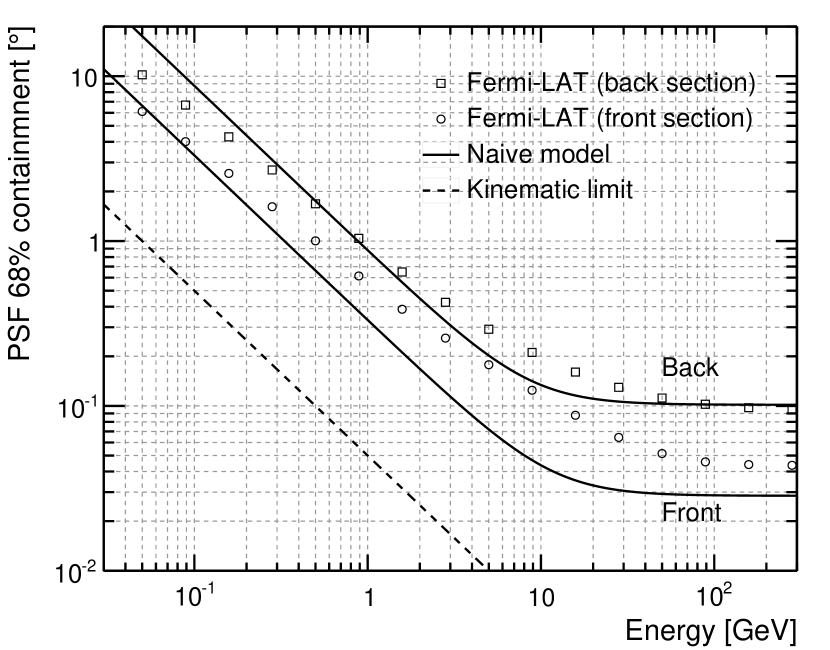
Figure 65: Comparison of our naïve estimates for the Fermi-LAT PSF with the output of a full Monte Carlo simulation of the detector. For reference the kinematic limit introduced in section VII.3.1 is also shown.

That all said, our angular resolution is just the sum in quadrature of the two terms:

$${\sigma_{\theta}}_{\rm F/B}={\sigma_{\theta}}_{\rm F/B}^{\rm MS}\oplus{\sigma_{\theta}}_{\rm F/B}^{\rm hit}$$ (103)

and this can be compared directly with the $68\%$ containment of the PSF, as shown in figure 65. The fact that our model is within a factor of two or so from the full detector Monte Carlo simulation over some four orders of magnitude is remarkable, given all the things that we have (brutally) neglected.

X Design principles

Not surprisingly, the question of how one should design a scientific instrument (be it for space or not) is a tough one—and one that requires many different inputs. The typical logical flow is to start with a precise idea of the science targets, i.e., what we want to measure. The science requirements translate more or less obviously into corresponding requirements on the detector performance, e.g., acceptance, point-spread function and energy resolution. How to turn them into an actual instrument implementation that fits into all the operational constraints (e.g., the weight and dimensions that can be accommodated by the launcher and the power budget) is often the most difficult part of the process—and one might have to iterate the process itself several time for it to converge.

In this section we shall briefly glance through some of the basic aspects of instrument design. (And no, even if you do read the section all the way to its end you should not go out and try and design your own space detector right away.)

X.1 Sensitivity studies

Now that we have a basic understanding of the main figures of merit describing the instrument performance it is time to try and tie them to the actual things that one aims at measuring.

X.1.1 Observing time, exposure factor and exposure

Up to now we haven’t quite talked about the observing time, but it is rather intuitive that the total number of events collected by a given instrument is proportional to the the exposure factor

$$\mathcal{E}_{\rm f}(E)=G(E)\times T_{\rm obs},$$ (104)

i.e., the product of the acceptance and the exposure factor (measured, e.g., in m² sr year). In passing, by “observing time”, here, we really mean the cumulative amount of time that the instrument is collecting science data. When defining the observing time, care should be taken to account for all the possible effects that reduce the overall duty-cycle: instrumental dead time, time spent for calibrations and hardware problems (and, for instruments in low-Earth orbit, the time spent in the SAA). And, since we are only concerned with the orders of magnitude, we shall obviously neglect all that in the following.

That all said, the exposure factor defined in (104) is mainly relevant for charged cosmic rays, whose flux is, to an good approximation, isotropic. On the other hand gamma-ray astronomy is by its nature dispersive—you see a subset of the sky at a time. What matters is the exposure $\mathcal{E}$, or the integrated effective area in a given direction in the sky—measured in m² year.

This is where the observation strategy comes into play: depending on how large is the field of view, aiming at a uniform exposure (i.e., scanning the sky) vs. pointing a particular region can give very different answers. Phrased in a different way, different (and mutually exclusive) observing strategies potentially provide very different sensitivities for particular science objectives, so this is really an important piece of the puzzle.

Even in sky-survey mode, the exposure factor are the exposure are two very different things: assuming that the observation strategy provides an approximately uniform sky exposure on long time scales (which is the case, e.g., for Fermi), the two quantities are related to each other by

$$\mathcal{E}(E)\sim\frac{\mathcal{E}_{\rm f}(E)}{4\pi}=\frac{G(E)\times T_{\rm obs}}{4\pi}.$$ (105)

It follows that an overall exposure factor of 1 m² sr year and an exposure of 1 m² year in a given direction in the sky are fundamentally different things: for an instrument with an acceptance of 1 m² sr it takes 1 year of observation to achieve the former and about $12.5$ year for the latter.

X.1.2 Cosmic-ray and gamma-ray intensities

We are now ready to attack some basic sensitivity studies. The first obvious case is calculating the expected number of cosmic rays of a particular species (e.g., protons or electrons) for a given detector acceptance and observing time. One obvious follow-up question would be what is the maximum energy up to which a given detector can study a given component of the cosmic radiation before running out of statistics.

One possible way to go about this—given a model for the differential intensity $J(E)$ under study—is to calculate the integral number of events $N_{I}$ above a given energy:

$$N_{I}(E)=\int_{E}^{\infty}\!\!\!\!\mathcal{E}_{\rm f}(E^{\prime})J(E^{\prime})dE^{\prime}.$$ (106)

(Check for yourself that all the physical units cancel out and the result is a pure number.) Compared to the corresponding differential quantity this has the advantage of depending on a single energy bound.

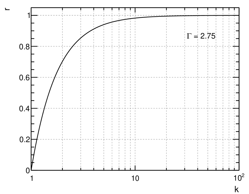
Figure 66: Accuracy of the integral spectra evaluation as a function of the upper extreme of integration, as given in equation 107.

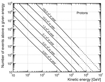
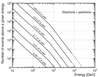
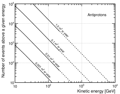
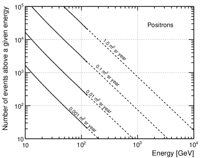
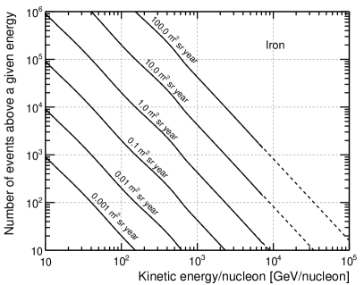
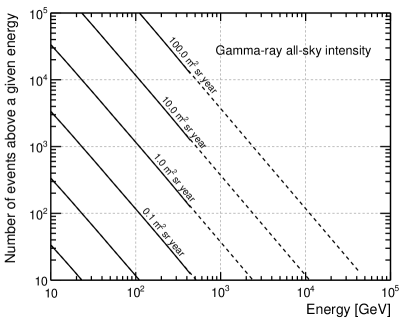
Figure 67: Integral number of events above a given energy for some interesting CR species, and for some representative values of the exposure factor. As a rule of thumb we can fairly say that, for each species, the energy for which a given curve drops below $\sim 10$ is the ultimate energy reach for an instrument integrating the corresponding exposure factor. Note that the axis ranges are all different. Also note that, for obvious reasons, the spectrum extrapolations are quite uncertain for the positrons.

We note, in passing, that the upper extreme of integration in equation (106) is formally infinite, but given how steeply cosmic-ray spectra are falling down, one hardly needs to get that far. For a power law with index $\Gamma$ the relevant figure is the ratio

$$r=\frac{\int_{E}^{kE}E^{\prime-\Gamma}dE^{\prime}}{\int_{E}^{\infty}E^{\prime-\Gamma}dE^{\prime}}=1-\frac{1}{k^{\Gamma-1}},$$ (107)

which is plotted in figure 66 for $\Gamma=2.75$. Integrating over a decade in energy is in practice enough to get us within a few % of the exact answer and a factor of $\sim 3$ in energy still provides an answer accurate to some $\sim 15\%$. This implies that, in order to evaluate the integral spectra above a given energy $E$, one needs a reliable estimation of the corresponding differential intensities up to energy at least 3–4 times higher.

If the exposure factor does not depend on energy, which is not a terrible assumption for most high-energy instruments, at least under certain conditions, the problem simplifies considerably

$$N_{I}(E)=\mathcal{E}_{\rm f}\int_{E}^{\infty}\!\!\!\!J(E^{\prime})dE^{\prime},$$ (108)

as by integrating the differential intensity one effectively gets a universal function that can be scaled by the exposure factor and plotted for different values of $\mathcal{E}_{\rm f}$ as shown in figure 67.

When looking at figure 67 the reader should be aware that the we have used our naïve baseline models of cosmic-ray intensities, and we have extrapolated them at high energy—which means that the numbers you read off the plot cannot expected to be accurate to three significant digits. That said, the plots allow to have a good idea of how many particles one is expecting to detect in a given setup above a given energy—and, by difference, in any given energy range.

The energy value for which the curve of interest in figure 67 falls below, say, 10 events signal the maximum energy reach that one might hope to reach for a given cosmic-ray species with a given exposure factor. Depending on the situation this might be realistic or no—e.g., a measurement with a magnetic spectrometer might be dominated by the charge confusion well before reaching out that far. In other words one should always keep in mind figure 50 when looking at figure 67.

X.1.3 Gamma-ray source sensitivity

As one might imagine, evaluating the source sensitivity for a given instrument involves a fair number of ingredients—most notably the effective area and point-spread function of the detector, the observation time toward a given direction in the sky and the intensity of the isotropic and galactic diffuse emission around the very same direction. In broad terms the detection threshold (i.e., the minimum integral source flux above a given energy $E_{\rm min}$ that is needed to detect the source itself at a given position and in a given observation time $T_{0}$) is determined by the number of background events—i.e., gamma rays from diffuse emission—into the solid angle subtended by the (energy-dependent) PSF. It goes without saying that the detection threshold depends on the position in the sky and is largest where the galactic diffuse emission is most intense (e.g., on the galactic plane and especially around the galactic center).

If we assume that the diffuse background is locally uniform, it is possible to derive an approximate expression for the detection threshold. In the following we shall outline a prescription described in Abdo et al. (2010b) in the context of the Fermi-LAT first source catalog.

The basic starting point is the maximum likelihood formalism customarily used for gamma-ray source analysis—described, e.g., in Mattox et al. (1996). The likelihood of observing $n_{i}$ counts in the $i$-th bin (here the pixel index $i$ is running in space and energy) where the model predicts $\lambda_{i}$ counts is given by the Poisson probability

$$p_{i}=\frac{\lambda_{i}^{n_{i}}e^{-\lambda_{i}}}{n_{i}!}.$$ (109)

The full likelihood is the product of the (independent) probabilities for each single pixels

$$L=\prod_{i}p_{i}=\prod_{i}\frac{\lambda_{i}^{n_{i}}e^{-\lambda_{i}}}{n_{i}!}$$ (110)

and the log-likelihood reads

$$\ln L=\sum_{i}\left(n_{i}\ln\lambda_{i}-\lambda_{i}-\ln n_{i}!\right).$$ (111)

The last term is irrelevant as it does not depend on the model, and the quantity that we have to maximize is effectively

$$\ln L=\sum_{i}\left(n_{i}\ln\lambda_{i}-\lambda_{i}\right).$$ (112)

Finally, the test statistics (roughly speaking, the square of the significance of the detection) is given by (twice) the difference between the likelihood with the source included in the model and the likelihood calculated under the hypothesis of no source:

$${\rm TS}=2(\ln L^{*}-\ln L^{0}).$$ (113)

Assuming a locally uniform background we can rewrite the above expression in the form of an integral over the energy and the angular separation $\psi$ between the source position and the reconstructed direction. Let $S(E)$ be the spectrum of the source, $B(E)$ that of the background, ${\rm PSF}(E,\psi)$ the spatial distribution of the events from a point source (at a given energy); in addition, let us define the local source-to-background ratio

$$g(E,\psi)=\frac{S(E){\rm PSF}(E,\psi)}{B(E)}.$$ (114)

That all said, the probability density function for the number of events detected will be

$$n*(E,\psi) =T_{0}A_{\rm eff}(E)\left(S(E){\rm PSF}(E,\psi)+B(E)\right)$$

$$=T_{0}A_{\rm eff}(E)B(E)(1+g(E,\psi))$$ (115)

if the source is included and

$$n^{0}(E,\psi)=T_{0}A_{\rm eff}(E)B(E)$$ (116)

in case of no source (note that both have to be integrated in energy and solid angle to get the actual number of events in the two hypotheses). The corresponding differential TS contribution per unit energy and solid angle reads

$$\frac{d{\rm TS}}{dEd\Omega} =2\left[(n^{*}\ln n^{*}-n^{*})-(n^{*}\ln n^{0}-n^{0})\right]=$$

$$=2\left[n^{*}\ln\left(\frac{n^{*}}{n^{0}}\right)-(n^{*}-n^{0})\right]=$$

$$=2T_{0}A_{\rm eff}(E)B(E)\times$$

$$\Big{[}(1+g(E,\psi))\ln(1+g(E,\psi))-g(E,\psi)\Big{]}.$$

Assuming a given spectral shape for $S(E)$, e.g., a power law with a given index, and a model for the diffuse emission e.g., the GDE model that we have introduced in section IV.3.1, one can integrate over the energy and the solid angle to get the actual TS and calculate the value of the minimum required normalization of the source spectrum—for a $5\sigma$ detection—by setting ${\rm TS}=25$.

Complicated as it might seems, the previous expression simplifies considerably in the background-dominated regime, i.e., when $g(E,\psi)\ll 1$ even for $\psi=0$. By expanding

$$(1+x)\ln(1+x)-x\sim(1+x)\left(x-\frac{x^{2}}{2}\right)-x\sim\frac{x^{2}}{2}$$ (117)

one gets the approximate relation

$$\frac{d{\rm TS}}{dEd\Omega}\sim\frac{T_{0}A_{\rm eff}(E)S(E)^{2}{\rm PSF}(E,\psi)^{2}}{B(E)}.$$ (118)

Finally, by noting that

$$\int_{0}^{\pi}{\rm PSF}(E,\psi)d\Omega\propto\frac{1}{\sigma(E)^{2}},$$ (119)

where $\sigma(E)$ is the angular resolution at a given energy $E$, one recognizes in the TS contribution per unit energy

$$\frac{d{\rm TS}}{dE}\propto\frac{T_{0}A_{\rm eff}(E)S(E)^{2}}{B(E)\sigma(E)^{2}}\propto\frac{n_{\rm sig}^{2}}{n_{\rm bkg}^{\rm eff}}$$ (120)

the (square of) the number of signal events divided by the square root of the number of background events within the solid angle subtended by the PSF of the instrument.

We refer the reader to Abdo et al. (2010b) for a more thorough description of the procedure in the specific case of the Fermi Large Area Telescope.

X.1.4 Search for spectral lines

The detection of a high-energy spectral line on top of the continuum gamma-ray emission (e.g., from the galactic center), is generally regarded as one of the few instances of a potential observable phenomenon that would convincingly point to the existence of new physics at work (e.g., two-body annihilation of dark matter into photons). The topic has recently received a lot of attention due to the claim Bringmann et al. (2012); Weniger (2012) of a line-like feature around 130 GeV in the publicly available Fermi data.

From the standpoint of what we are interested in, the general subject of the line search provides a good example to underline the interplay between the acceptance and the energy resolution in this specific analysis. In broad terms, the basic figure of merit $Q$ for such a line search is

$$Q=\frac{n_{s}}{\sqrt{n_{b}}},$$ (121)

where $n_{s}$ is the number of signal events and $n_{b}$ is the effective background, i.e. the number of background events integrated over the signal p.d.f. At a fixed signal flux and detector acceptance, both the signal and the background scale linearly with the exposure factor $\mathcal{E}_{\rm f}$, but the width of the window over which the background is integrated is proportional to the energy resolution, which implies that

$$Q\propto\sqrt{\frac{\mathcal{E}_{\rm f}}{\frac{\sigma_{E}}{E}}}.$$ (122)

While a good energy resolution is surely desirable for this particular search, equation (122) implies that the sensitivity increases with a narrower energy dispersion only if one is not trading too much acceptance for that.

X.2 Operational constraints

Delving into the details of the instrument design principles from the standpoint of the operational constraints is obviously beyond the scope of the write-up. Nonetheless we shall glance through some of the most obvious aspects of the problem, with emphasis on space-based detectors.

X.2.1 Weight, power and all that

The first obvious constraints imposed by the choice of the launcher are on the overall dimensions and weight of the instrument. The latter impacts primarily the layout of the calorimeter, which typically accounts for a significant fraction of the mass in most popular instrument designs. In broad terms, once the calorimeter weight is fixed, one has the face a trade off between the acceptance and the energy resolution—i.e., decide the optimal compromise between the cross-sectional active surface and the depth. It should be emphasized that for magnetic spectrometers the magnet is also a fundamental contributor to the mass budget.

Power in space generally comes from solar panels—and is not unlimited. Typical power budgets for space- and balloon-borne detectors are within 500–1000 W—rarely much more than that. In terms of detector implementation, the limited power primarily impacts the tracking stage, which is typically the one featuring the highest level of segmentation (as we mentioned in section VIII.1.2, silicon trackers with $10^{5}$–$10^{6}$ independent electronic channels are nowadays commonly operated in space).

The bandwidth for data down-link is expensive, too—pretty much as anything else in space—with typical average figures ranging in the Mb/s. This has profound implication on the overall data flow, requiring in general some combination of zero suppression, event filtering and data compression (all happening on board).

X.2.2 Launch and space environment

In contrast to ground-based detectors (e.g., experiments at accelerators), space-based instruments must be designed, assembled and tested as to ensure successful launch and on-orbit operation. The environmental verification process typically includes mechanical tests (both static and dynamic), thermal tests (thermal and/or thermo-vacuum cycling) and electromagnetic emission and susceptibility tests. While this general topic is not trivial to discuss without reference to a specific instrument, we shall briefly introduce some of the basic aspects of the problem. The reader is referred, e.g., to Bagagli et al. (2008) for a thorough discussion of the environmental tests of the Fermi-LAT tracker towers.

Vibration tests are aimed at verifying that the detector can sustain the low-frequency dynamic load in the launch environment—i.e., vibrations induced by the bearing structures (the satellite and the launcher) at the natural frequencies of the latter (usually below 50 Hz). The transfer function of the instrument assembly (or any of its sub-parts) is typically measured by means of a combination of a shaker and a series of accelerometers, that allow to measure both the resonance frequencies and the $Q$ factors of the natural modes (and verify that they do not change significantly in response to a realistic simulation of the launch environment, which might indicate some kind of structural damage).

In the space environment heat is exchanged between the detector and the ambient essentially by radiation (it goes without saying that convection plays no role in vacuum, which means that you can’t really use fans to dissipate heat as you would do on the ground). Space-based detectors feature more or less sophisticated thermal systems to ensure that the power generated by the on-board electronics is efficiently radiated in the environment and to mitigate the thermal gradients induced by changes of the orientation with respect to the Sun (and Sun occultation by the Earth). Thermal and thermo-vacuum tests serve the twofold purpose of validating the thermal model at the base of the thermal control system and verifying that the detector is able to operate (or survive) withing the maximum temperature excursion range expected in orbit.

We note, in passing, that operating an instrument in vacuum is not as trivial as one might expect, as in many designs composite structures (i.e., aggregates of several layers of different materials) are used in order to maximize the mechanical stiffness within the mass budget—and the details of manufacturing processes become critical.

There are many more considerations—connected with the environment—that go into the design of a space detector (e.g., electromagnetic interference effect and radiation damage) but we shall just pause here and move forward to a different subject.

X.3 Design trade-offs

Trade-offs arise naturally when designing an instrument, as—even pretending for a second that the operational constraints do not exist—it is impossible to optimize all the performance metrics at the same time and it is necessary to do compromises aimed at maximizing the overall sensitivity for a given science target. In addition to that, different science targets may require different (and often conflicting) optimizations, which makes the entire process even more difficult.

In this section we shall elaborate on the concept of trade-off by looking at a couple of (largely) academic examples.

X.3.1 A case study: the tracking stage for a pair-conversion telescope

Let’s pretend for a second that your favorite space agency contacted you to design the tracking stage for a pair-conversion telescope. The rules are: you have a cubic space, with side $L=1$ m, to fill up (completely) with $n$ equally-spaced aggregates, each including a double-sided silicon-strip detection plane with strip pitch $p$, immediately followed by a high-Z converter with thickness $t$. (In other words, you have 1 m³ available and you get to pick your favorite choices for $n$, $p$ and $t$.) Last but not least, the agency is offering you a non-negotiable power budget of 100 W.

There’s a few performance metrics that we can calculate right away. Assuming a 100% detection and selection efficiency, for instance, the peak (i.e., high-energy) on-axis effective area can be estimated as

$$A_{\rm eff}^{\perp}=L^{2}[1-\exp(-nt)]=1-\exp(-nt)~{}{\rm m}^{2}.$$ (123)

In addition, following section IX.5.1, we can write the high-energy 68% containment angle of the PSF as

$${\rm PSF}_{\rm HE}=\frac{\sqrt{2}p}{d(n/2)^{3/2}}=\frac{4p}{Ln^{1/2}}=\frac{p~{}[\mu{\rm m}]}{250n^{1/2}}~{}{\rm mrad}$$ (124)

(note we are taking $n/2$ as the average number of planes crossed). The corresponding PSF at 100 MeV reads

$${\rm PSF}_{100}=\sqrt{2}\frac{13.6}{50}\sqrt{t}=385\sqrt{t}~{}{\rm mrad}$$ (125)

(note we have neglected the extra logarithmic term in equation (40)).

That all said, with three free parameters it is not trivial to imagine how one would go about the optimization. One thing that we can easily calculate is the overall number of channels:

$$\text{\# channels}=\frac{2nL}{p}$$ (126)

(the factor 2 at the numerator accounts for the fact that, for each plane, we have strips in both directions—i.e., the silicon detectors are double sided). If we assume a power consumption of 250 $\mu$W per channel, the total necessary power $P$ reads

$$P=\frac{500n}{p~{}[\mu{\rm m}]}~{}W,$$ (127)

i.e., with 100 W available you can do, say, 10 layers at 50 $\mu$m pitch or 100 layers at 500 $\mu$m pitch (see the right axis in figure 68). Good: this introduces a constraint that our design parameters must satisfy

$$p=5n~{}\mu{\rm m},$$ (128)

and effectively reduces the dimensionality of the problem from 3 to 2. In fact we can now rewrite the high-energy PSF as

$${\rm PSF}_{\rm HE}=\frac{n^{1/2}}{50}~{}{\rm mrad}$$ (129)

(if you are surprised seeing that the PSF is worsening as one adds more layers, remember that the power budget is forcing us to make the strip pitch larger).

Figure 68 summarizes this trade-off study in the $n$–$t$ plane. In our setup the low-energy PSF depends only on the thickness of the converters and the high-energy PSF depends only on the number of layers (which in turn, at fixed total power, determines the strip pitch). Hyper-surfaces at constant on-axis high-energy effective area are represented by the dashed curves.

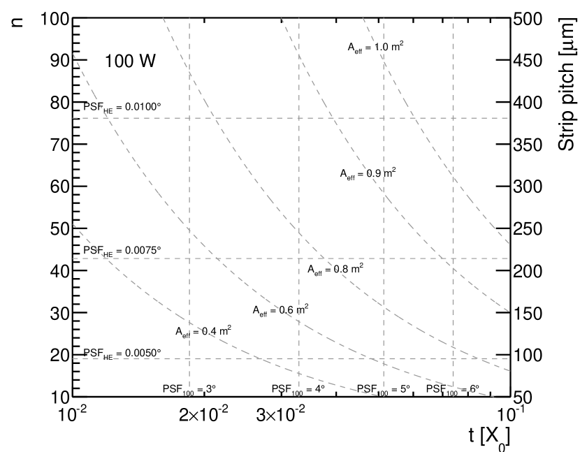
Figure 68: Iso-performance curves in the $n$–$t$ phase space for our benchmark pair conversion telescope. The lines at constant ${\rm PSF}_{100}$ are vertical, while those at constant ${\rm PSF}_{\rm HE}$ are horizontal. The curves are iso-$A_{\rm eff}$ lines.

There’s a few interesting remarks that we can do about figure 68. Obviously one would like to choose a small value of $t$ to optimize the PSF at low energy. In addition, in our setup it is advantageous to limit the number of detection planes and take advantage of the smaller strip pitch to optimize the high-energy PSF. By choosing the bottom-left corner of the phase space one effectively optimizes the angular resolution over the entire energy range. Unfortunately this is also the region where the effective area is relatively low (no wonder: you have a small number of thin conversion layers). In contrast, increasing the effective area requires trading off some angular resolution, at either low or high energies—or both.

There is several things that we left off, including cost considerations and other performance metrics such as the field of view. Nonetheless, fictional as it is, this exercise does illustrates some of the basic aspects of instrument design.

XI In-flight calibration

Space- and balloon-borne detectors are typically calibrated with particle beams prior to launch in order to benchmark the Monte Carlo simulations used to generate the instrument response function. While this is of primary importance, one should recognize that that the space environment is different, to many respects, than that in which ground tests are performed. In addition, cosmic-ray and gamma-ray detector often aim at measuring fluxes and intensities at much higher energies that those accessible by accelerators.

In this section we shall glance through the topic of in-flight instrument calibration. There are two main aspects to this—namely the monitoring of the performance stability in time and the assessment of the systematic uncertainties associated to the instrument response functions (e.g., effective area, point-spread function and absolute energy scale). As we shall see in a second, the latter is generally much harder—and it goes without saying that it is more critical for satellite (as opposed to balloon) experiments, since, due the much larger exposure factors, many of the measurements are systematic-limited.

XI.1 Time stability

The stability in time of the basic instrument performance figures is usually monitored both through dedicated calibration systems embedded in the readout electronics (e.g., charge-injection circuits to measure the gain and noise of the front-end amplifiers, or laser systems to measure the alignment of tracking devices) and using the particle populations available in orbit. In this latter respect minimum ionizing protons are a good example of an abundant calibration source with well-known properties that can be used by large-acceptance detectors to monitor the performance stability over relatively short time-scales.

Figure 69 shows the relative light yield of the Fermi-LAT calorimeter, measured through the first four years of mission by means of the path-length-corrected energy deposition of on-orbit minimum ionizing protons Bregeon et al. (2013). The slight ($\sim 1\%$ per year) downward trend (due to the anticipated radiation damage of the CsI crystals) is a good example of an effect that, if not corrected through time-dependent calibrations, might produce observable consequences in the high-level science analysis—first and foremost a drift of the absolute energy scale. (On a related note, it is worth noticing that it’s easier to use minimum-ionizing proton to monitor the stability of the energy scale, rather than calibrating it directly.)

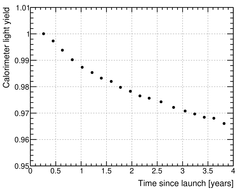
Figure 69: Relative light yield for the Fermi-LAT calorimeter, inferred from the path-length-corrected energy deposition of on-orbit minimum ionizing protons, throughout the first four years of the mission (adapted from Bregeon et al. (2013)). The small downward trending is due to the (expected) radiation damage of the calorimeter crystals.

The on-orbit refinement and monitoring of the AMS-02 tracker alignment described, e.g., in Ambrosi and et al. (2013b) constitutes another interesting topic of discussion germane to the main subject of this section. As we know, by now, for magnetic spectrometers the tracker alignment is crucial, as the high-energy rigidity resolution is hostage to the spatial resolution in the bending plane. In the case of AMS-02 is impressive how the instrument team managed to cope with the time-dependent displacements of the outer tracker layers induced by temperature variation (up to hundreds of $\mu$m on sub-hour time scales) and achieve a systematic error on the alignment of the order of $\sim 3~{}\mu$m—significantly smaller than the hit resolution of the position-sensitive detectors.

XI.2 Systematic uncertainties on the IRFs

Measurements by modern, large-acceptance detectors are in many (possibly most) cases systematic-limited—one has so many events at hand that the statistical errors are just negligible over most of the instrumental phase space. When that is the case the level of accuracy of our knowledge of the detector performance figures (i.e., the systematic errors on the instrument response functions) becomes, to some extent, more important than the absolute values of the figures themselves. It is important, therefore, to devise methods study those systematic errors in the environment where the instrument operates.

XI.2.1 Effective area and acceptance

The effective area is typically studied and parameterized by means of detailed Monte Carlo simulations and measured with particle beams, when possible, in discrete points of the phase space.

Given that there is no such thing as a source with a known flux (this is typically what one is trying to measure) it is not straightforward to study the systematic errors on the effective area on orbit. There are ways around this: one can select reasonably clean, signal-enriched event samples and study the efficiency of any given selection criterium with respect to a baseline; or try and measure the same thing with sub-samples of events—e.g., on-axis and off-axis events. We refer the reader to Ackermann et al. (2012c) for a somewhat detailed discussion of such possible strategies in the context of the analysis of Fermi-LAT gamma-ray data, but we stress that this is a difficult problem to discuss in abstract terms.

XI.2.2 Point-spread function

The point-spread function is, to some extent, the easiest thing to calibrate in orbit (at least where it matters, i.e., in gamma rays), in that bright gamma-ray point sources serve essentially the same purpose that a monochromatic particle beam would serve for energy calibration: not only the measured photon directions are distributed around the true position according to the PSF (this is by definition), but in many cases this true position is known from measurements at other wavelengths.

Bright pulsars are prototypical examples of sources that can be used for the in-flight calibration of the PSF—in that case one can also take advantage the phase information to select the calibration sample. One notable limitation is due to the fact that most pulsars feature a spectral cutoff at $\sim$ GeV energy, so that they cannot be readily used at very high energies. Bright active galactic nuclei (and possibly a stack of them) are a viable alternatives. We refer the reader to Ackermann et al. (2012c, 2013b) for a thorough discussion of the in-flight calibration of the Fermi-LAT PSF.

XI.2.3 Absolute energy scale

Unlike the point-spread function, the absolute energy scale is notoriously difficult to calibrate in orbit due to the lack of sharp spectral features at know energies in the GeV-to-TeV range. As a matter of fact, the discovery of such a feature (e.g., a line) would be a major one, but still useless from the standpoint of the calibration of the energy scale.

Magnetic spectrometers with an electromagnetic calorimeter on board have the advantage of measuring the energy and the rigidity (which is to say, they measure the energy twice and independently) for electrons and positrons with a good resolution over a relatively wide energy range. The energy-rigidity matching provides a good handle on the systematic uncertainties on the absolute scales, but for purely calorimetric experiments life is relatively harder.

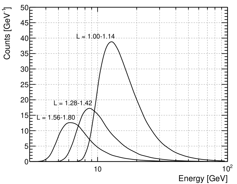
Figure 70: Examples of simulated cosmic-ray electron count spectra in bins of McIlwain $L$, representative of the Fermi orbit—averaged over the FermiLAT field of view and folded with the FermiLAT energy resolution (adapted from Ackermann et al. (2012d)). The peaked shape is the result of the convolution of the power-law spectrum of primary cosmic-ray electrons with the screening effect of the geomagnetic field. The different peaks at different values of McIlwain $L$, whose position can be reliably predicted through ray-tracing techniques, effectively provide a series of calibration points for the absolute energy scale.

We end this section by briefly mentioning the verification of the absolute energy scale performed by the Fermi-LAT Ackermann et al. (2012d) using the rigidity cutoff induced by the geomagnetic field (see section VI.2.4). While the geomagnetic cutoff is a sharp feature in any given direction, it gets smeared when averaged over the finite field of view of an instrument, as shown in figure 70. Still, by selecting events in bins of the McIlwain $L$ variable, the convolution between the power-law spectrum of primary cosmic-ray electrons and the shielding effect due to the magnetic field results in narrowly-peaked spectra whose shape can be predicted by means of ray-tracing techniques. We refer the reader to Ackermann et al. (2012d) for more details about the method and the results.

Change log

We are trying and log in this section the most relevant changes that are done to the manuscript as it evolves. Cross-links are in the context of the most recent version of the write-up where possible.

Version v2, last edited on August 4, 2014

• Filled in some more numbers in table 4—most notably Gamma-400 and HERD were added.

• Added $z$-axis labels to figures 23, 24 and 27.

Appendix A Cosmic-ray measurements

Table 11: List of cosmic-ray measurements from Maurin et al. (2013), ordered by particle type and by year within each type.

Experiment	Energy range	Date	Reference
10B/11B
AMS01	0.20–1.4 [GeV/n]	1998 Jun 02–1998 Jun 12	Aguilar et al. (2011)
ISOMAX	0.28–0.95 [GeV/n]	1998 Aug 04–1998 Aug 05	Hams et al. (2004)
10B/B
Balloon	0.16–0.42 [GeV/n]	1973 Aug 15–1973 Aug 15	Hagen et al. (1977)
Voyager1&2	0.04–0.12 [GeV/n]	1977 Jan 01–1998 Dec 31	Lukasiak (1999)
Voyager1&2	0.04–0.12 [GeV/n]	1977 Jan 01–1996 Dec 31	Lukasiak et al. (1997a)
Balloon	0.26–1.6 [GeV/n]	1977 May 28–1977 May 29	Buffington et al. (1978)
Balloon	0.26–0.43 [GeV/n]	1977 Sep 01–1977 Sep 03	Webber and Kish (1979)
ISEE3-HIST	0.03–0.11 [GeV/n]	1978 Aug 13–1978 Dec 01	Mewaldt et al. (1981)
ISEE3-HKH	0.09–0.17 [GeV/n]	1978 Aug 14–1981 Apr 03	Krombel and Wiedenbeck (1988)
HEIST	0.41–0.64 [GeV/n]	1988 Aug 25–1988 Aug 27	Gibner et al. (1992)
10Be/9Be
Balloon	0.16–0.42 [GeV/n]	1973 Aug 15–1973 Aug 15	Hagen et al. (1977)
IMP7&8	0.03–0.15 [GeV/n]	1974 Jan 01–1980 May 23	Garcia-Munoz et al. (1981)
Voyager1&2	0.04–0.11 [GeV/n]	1977 Jan 01–1998 Dec 31	Lukasiak (1999)
Balloon	0.20–1.5 [GeV/n]	1977 May 28–1977 May 29	Buffington et al. (1978)
Balloon	0.20–0.33 [GeV/n]	1977 Sep 01–1977 Sep 03	Webber and Kish (1979)
ISEE3-HKH	0.06–0.18 [GeV/n]	1978 Aug 14–1979 Aug 18	Wiedenbeck and Greiner (1980)
Ulysses-HET	0.07–0.14 [GeV/n]	1990 Oct 07–1997 Dec 01	Connell (1998)
ACE-SIS	0.02–0.07 [GeV/n]	1997 Aug 28–1999 Jul 08	Yanasak et al. (2001)
ACE-CRIS	0.07–0.14 [GeV/n]	1997 Aug 28–1999 Jul 08	Yanasak et al. (2001)
ISOMAX	0.26–2.0 [GeV/n]	1998 Aug 04–1998 Aug 05	Hams et al. (2004)
10Be/Be
IMP7&8	0.03–0.15 [GeV/n]	1972 Sep 01–1975 Sep 30	Garcia-Munoz et al. (1977)
Balloon	0.16–0.42 [GeV/n]	1973 Aug 15–1973 Aug 15	Hagen et al. (1977)
IMP7&8	0.03–0.15 [GeV/n]	1974 Jan 01–1980 May 23	Garcia-Munoz et al. (1981)
Voyager1&2	0.04–0.09 [GeV/n]	1977 Jan 01–1998 Dec 31	Lukasiak (1999)
Voyager1&2	0.04–0.09 [GeV/n]	1977 Jan 01–1996 Dec 31	Lukasiak et al. (1997a)
Voyager1&2	0.04–0.11 [GeV/n]	1977 Jan 01–1991 Dec 31	Lukasiak et al. (1994a)
Balloon	0.17–1.1 [GeV/n]	1977 May 28–1977 May 29	Buffington et al. (1978)
Balloon	0.20–0.33 [GeV/n]	1977 Sep 01–1977 Sep 03	Webber and Kish (1979)
ISEE3-HKH	0.06–0.18 [GeV/n]	1978 Aug 14–1979 Aug 18	Wiedenbeck and Greiner (1980)
Ulysses-HET	0.07–0.14 [GeV/n]	1990 Oct 07–1997 Dec 01	Connell (1998)
11B/B
Balloon	0.14–0.39 [GeV/n]	1970 Jun 01–1970 Jun 01	Bjarle et al. (1979)
Balloon	0.16–0.42 [GeV/n]	1973 Aug 15–1973 Aug 15	Hagen et al. (1977)
Voyager1&2	0.04–0.11 [GeV/n]	1977 Jan 01–1998 Dec 31	Lukasiak (1999)
Voyager1&2	0.04–0.11 [GeV/n]	1977 Jan 01–1996 Dec 31	Lukasiak et al. (1997a)
Balloon	0.22–1.4 [GeV/n]	1977 May 28–1977 May 29	Buffington et al. (1978)
Balloon	0.24–0.40 [GeV/n]	1977 Sep 01–1977 Sep 03	Webber and Kish (1979)
12C/C
IMP7&8	0.04–0.07 [GeV/n]	1973 Feb 01–1977 Sep 01	Guzik (1981)
Balloon	0.16–0.42 [GeV/n]	1973 Aug 15–1973 Aug 15	Hagen et al. (1977)
Balloon	0.26–1.6 [GeV/n]	1977 May 28–1977 May 29	Buffington et al. (1978)
Balloon	0.41–0.49 [GeV/n]	1977 Sep 01–1977 Sep 03	Webber (1982)
13C/12C
Voyager1&2	0.05–0.13 [GeV/n]	1977 Jan 01–1993 Dec 31	Webber et al. (1996)
ISEE3-HKH	0.10–0.30 [GeV/n]	1978 Aug 14–1980 May 03	Wiedenbeck and Greiner (1981a)
Voyager1&2	0.05–0.13 [GeV/n]	1986 Jan 01–1989 Dec 01	Lukasiak et al. (1994b)
HEIST	0.43–0.67 [GeV/n]	1988 Aug 25–1988 Aug 27	Gibner et al. (1992)
CRRES	0.10–0.20 [GeV/n]	1990 Jul 25–1992 Oct 12	Duvernois et al. (1996a)
13C/C
Balloon	0.14–0.39 [GeV/n]	1970 Jun 01–1970 Jun 01	Bjarle et al. (1979)
IMP7&8	0.04–0.07 [GeV/n]	1973 Feb 01–1977 Sep 01	Guzik (1981)
Balloon	0.16–0.42 [GeV/n]	1973 Aug 15–1973 Aug 15	Hagen et al. (1977)
Balloon	0.23–1.4 [GeV/n]	1977 May 28–1977 May 29	Buffington et al. (1978)
Balloon	0.39–0.47 [GeV/n]	1977 Sep 01–1977 Sep 03	Webber (1982)
ISEE3-HIST	0.03–0.13 [GeV/n]	1978 Aug 13–1978 Dec 01	Mewaldt et al. (1981)
14N/16O
Voyager1&2	0.06–0.15 [GeV/n]	1977 Jan 01–1993 Dec 31	Webber et al. (1996)
Voyager1&2	0.06–0.15 [GeV/n]	1986 Jan 01–1989 Dec 01	Lukasiak et al. (1994b)
CRRES	0.11–0.23 [GeV/n]	1990 Jul 25–1992 Oct 12	Duvernois et al. (1996a)
14N/N
IMP7&8	0.06–0.09 [GeV/n]	1973 Feb 01–1977 Sep 01	Guzik (1981)
Balloon	0.16–0.42 [GeV/n]	1973 Aug 15–1973 Aug 15	Hagen et al. (1977)
Balloon	0.26–0.90 [GeV/n]	1977 May 28–1977 May 29	Buffington et al. (1978)
Balloon	0.44–0.52 [GeV/n]	1977 Sep 01–1977 Sep 03	Webber (1982)
Balloon	0.38–0.45 [GeV/n]	1981 Sep 27–1981 Sep 28	Webber et al. (1985a)
15N/16O
Voyager1&2	0.06–0.15 [GeV/n]	1977 Jan 01–1993 Dec 31	Webber et al. (1996)
Voyager1&2	0.06–0.15 [GeV/n]	1986 Jan 01–1989 Dec 01	Lukasiak et al. (1994b)
CRRES	0.11–0.23 [GeV/n]	1990 Jul 25–1992 Oct 12	Duvernois et al. (1996a)
15N/N
IMP7&8	0.06–0.09 [GeV/n]	1973 Feb 01–1977 Sep 01	Guzik (1981)
Balloon	0.16–0.42 [GeV/n]	1973 Aug 15–1973 Aug 15	Hagen et al. (1977)
Balloon	0.05–1.6 [GeV/n]	1973 Sep 29–1974 May 08	Dwyer (1978)
Balloon	0.23–0.81 [GeV/n]	1977 May 28–1977 May 29	Buffington et al. (1978)
Balloon	0.42–0.50 [GeV/n]	1977 Sep 01–1977 Sep 03	Webber (1982)
ISEE3-HIST	0.03–0.15 [GeV/n]	1978 Aug 13–1978 Dec 01	Mewaldt et al. (1981)
ISEE3-HKH	0.10–0.20 [GeV/n]	1978 Aug 14–1981 Apr 03	Krombel and Wiedenbeck (1988)
Balloon	0.38–0.44 [GeV/n]	1981 Sep 27–1981 Sep 28	Webber et al. (1985a)
HEIST	0.45–0.68 [GeV/n]	1988 Aug 25–1988 Aug 27	Gibner et al. (1992)
CRRES	0.11–0.23 [GeV/n]	1990 Jul 25–1992 Oct 12	Duvernois et al. (1996a)
16O/O
Balloon	0.26–0.90 [GeV/n]	1977 May 28–1977 May 29	Buffington et al. (1978)
Balloon	0.45–0.58 [GeV/n]	1977 Sep 01–1977 Sep 03	Webber (1982)
Balloon	0.39–0.48 [GeV/n]	1981 Sep 27–1981 Sep 28	Webber et al. (1985a)
17O/16O
Voyager1&2	0.06–0.15 [GeV/n]	1977 Jan 01–1993 Dec 31	Webber et al. (1996)
ISEE3-HIST	0.03–0.15 [GeV/n]	1978 Aug 13–1978 Dec 01	Mewaldt et al. (1981)
ISEE3-HKH	0.09–0.23 [GeV/n]	1978 Aug 14–1980 May 03	Wiedenbeck and Greiner (1981b)
Voyager1&2	0.06–0.15 [GeV/n]	1986 Jan 01–1989 Dec 01	Lukasiak et al. (1994b)
HEIST	0.46–0.78 [GeV/n]	1988 Aug 25–1988 Aug 27	Gibner et al. (1992)
CRRES	0.12–0.24 [GeV/n]	1990 Jul 25–1992 Oct 12	Duvernois et al. (1996a)
17O/O
Balloon	0.23–0.81 [GeV/n]	1977 May 28–1977 May 29	Buffington et al. (1978)
Balloon	0.45–0.58 [GeV/n]	1977 Sep 01–1977 Sep 03	Webber (1982)
Balloon	0.39–0.47 [GeV/n]	1981 Sep 27–1981 Sep 28	Webber et al. (1985a)
18O/16O
Voyager1&2	0.06–0.15 [GeV/n]	1977 Jan 01–1993 Dec 31	Webber et al. (1996)
ISEE3-HIST	0.03–0.15 [GeV/n]	1978 Aug 13–1978 Dec 01	Mewaldt et al. (1981)
ISEE3-HKH	0.09–0.23 [GeV/n]	1978 Aug 14–1980 May 03	Wiedenbeck and Greiner (1981b)
Voyager1&2	0.06–0.15 [GeV/n]	1986 Jan 01–1989 Dec 01	Lukasiak et al. (1994b)
HEIST	0.46–0.78 [GeV/n]	1988 Aug 25–1988 Aug 27	Gibner et al. (1992)
CRRES	0.11–0.24 [GeV/n]	1990 Jul 25–1992 Oct 12	Duvernois et al. (1996a)
18O/O
Balloon	0.42–0.54 [GeV/n]	1977 Sep 01–1977 Sep 03	Webber (1982)
Balloon	0.38–0.46 [GeV/n]	1981 Sep 27–1981 Sep 28	Webber et al. (1985a)
19F/20Ne
CRRES	0.10–0.29 [GeV/n]	1990 Jul 25–1992 Oct 12	Duvernois et al. (1996a)
1H
Voyager1-HET	0.03–0.07 [GeV/n]	1977 Oct 04–1977 Nov 22	Webber and Yushak (1983)
ISEE3-MEH	0.04–0.14 [GeV/n]	1978 Aug 18–1979 Jan 01	Kroeger (1986)
ISEE3-MEH	0.04–0.14 [GeV/n]	1979 Jan 01–1980 Jan 01	Kroeger (1986)
ISEE3-MEH	0.04–0.14 [GeV/n]	1980 Jan 01–1981 Jan 01	Kroeger (1986)
ISEE3-MEH	0.04–0.14 [GeV/n]	1981 Jan 01–1982 Jan 01	Kroeger (1986)
ISEE3-MEH	0.04–0.14 [GeV/n]	1982 Jan 01–1983 Jan 01	Kroeger (1986)
ISEE3-MEH	0.04–0.14 [GeV/n]	1983 Jan 01–1984 Jan 01	Kroeger (1986)
ISEE3-MEH	0.04–0.14 [GeV/n]	1984 Jan 01–1985 Jan 01	Kroeger (1986)
Voyager2-HET	0.03–0.07 [GeV/n]	1987 Jan 01–1987 Dec 31	Seo et al. (1994)
IMAX92	0.18–208 [GeV/n]	1992 Jul 16–1992 Jul 17	Menn et al. (2000)
BESS93	0.18–2.4 [GeV/n]	1993 Jul 01–1993 Jul 01	Wang et al. (2002)
CAPRICE94	0.15–9.5 [GeV/n]	1994 Aug 08–1994 Aug 09	Boezio et al. (1999)
BESS97	0.21–21.5 [GeV/n]	1997 Jul 27–1997 Jul 27	Shikaze et al. (2007)
AMS01	0.22–199 [GeV/n]	1998 Jun 02–1998 Jun 12	Alcaraz et al. (2000a)
BESS98	0.21–117 [GeV/n]	1998 Jul 29–1998 Jul 29	Shikaze et al. (2007)
BESS99	0.21–21.5 [GeV/n]	1999 Aug 11–1999 Aug 12	Shikaze et al. (2007)
BESS00	0.21–21.5 [GeV/n]	2000 Aug 10–2000 Aug 11	Shikaze et al. (2007)
BESS-TeV	0.21–541 [GeV/n]	2002 Aug 07–2002 Aug 07	Shikaze et al. (2007)
PAMELA	0.12–0.57 [GeV/n]	2006 Jul 01–2007 Dec 31	Adriani et al. (2013b)
1H-bar
MASS91	3.7–24.1 [GeV/n]	1991 Sep 23–1991 Sep 23	Basini (1999)
IMAX92	0.25–3.2 [GeV/n]	1992 Jul 16–1992 Jul 17	Mitchell et al. (1996)
BESS93	0.20–0.60 [GeV/n]	1993 Jul 01–1993 Jul 01	Moiseev et al. (1997)
CAPRICE94	0.60–3.2 [GeV/n]	1994 Aug 08–1994 Aug 09	Boezio et al. (1997)
BESS95	0.17–1.4 [GeV/n]	1995 Jul 25–1995 Jul 25	Matsunaga et al. (1998)
BESS97	0.18–3.6 [GeV/n]	1997 Jul 27–1997 Jul 27	Orito et al. (2000)
CAPRICE98	3.2–49.1 [GeV/n]	1998 May 28–1998 May 29	Boezio et al. (2001a)
AMS01	0.30–3.7 [GeV/n]	1998 Jun 02–1998 Jun 12	AMS Collaboration et al. (2002)
BESS98	0.18–4.2 [GeV/n]	1998 Jul 29–1998 Jul 29	Maeno et al. (2001)
BESS99	0.18–4.2 [GeV/n]	1999 Aug 11–1999 Aug 12	Asaoka et al. (2002)
BESS00	0.18–4.2 [GeV/n]	2000 Aug 10–2000 Aug 11	Asaoka et al. (2002)
BESS-TeV	0.18–4.2 [GeV/n]	2002 Aug 07–2002 Aug 07	Haino et al. (2005)
BESS-PolarI	0.10–4.2 [GeV/n]	2004 Dec 13–2004 Dec 21	BESS Collaboration et al. (2008)
PAMELA	0.12–179 [GeV/n]	2006 Jul 01–2009 Dec 01	Adriani et al. (2013a)
PAMELA	0.12–179 [GeV/n]	2006 Jul 01–2008 Dec 01	Adriani et al. (2010)
BESS-PolarII	0.17–3.5 [GeV/n]	2007 Dec 22–2008 Jan 19	Abe et al. (2012)
1H-bar/1H
MASS91	3.7–19.0 [GeV/n]	1991 Sep 23–1991 Sep 23	Hof et al. (1996)
IMAX92	0.25–3.2 [GeV/n]	1992 Jul 16–1992 Jul 17	Mitchell et al. (1996)
BESS93	0.20–0.60 [GeV/n]	1993 Jul 01–1993 Jul 01	Moiseev et al. (1997)
CAPRICE94	0.60–3.2 [GeV/n]	1994 Aug 08–1994 Aug 09	Boezio et al. (1997)
BESS95	0.17–1.4 [GeV/n]	1995 Jul 25–1995 Jul 25	Matsunaga et al. (1998)
BESS97	0.18–3.6 [GeV/n]	1997 Jul 27–1997 Jul 27	Orito et al. (2000)
CAPRICE98	3.2–49.1 [GeV/n]	1998 May 28–1998 May 29	Boezio et al. (2001a)
BESS98	0.18–4.2 [GeV/n]	1998 Jul 29–1998 Jul 29	Maeno et al. (2001)
BESS99	0.18–4.2 [GeV/n]	1999 Aug 11–1999 Aug 12	Asaoka et al. (2002)
HEAT-pbar	3.7–24.1 [GeV/n]	2000 Jun 03–2000 Jun 03	Beach et al. (2001)
BESS00	0.18–4.2 [GeV/n]	2000 Aug 10–2000 Aug 11	Asaoka et al. (2002)
BESS-TeV	0.18–4.2 [GeV/n]	2002 Aug 07–2002 Aug 07	Haino et al. (2005)
BESS-PolarI	0.18–4.2 [GeV/n]	2004 Dec 13–2004 Dec 21	BESS Collaboration et al. (2008)
PAMELA	0.12–179 [GeV/n]	2006 Jul 01–2009 Dec 01	Adriani et al. (2013a)
PAMELA	0.13–179 [GeV/n]	2006 Jul 01–2008 Dec 01	Adriani et al. (2010)
PAMELA	1.5–99.0 [GeV/n]	2006 Jul 01–2008 Jun 15	Adriani et al. (2009b)
20Ne/Ne
Voyager1&2	0.07–0.15 [GeV/n]	1977 Jan 01–1996 Dec 31	Webber et al. (1997)
CRISIS	0.39–0.53 [GeV/n]	1977 May 20–1977 May 22	Freier et al. (1980)
Balloon	0.44–0.59 [GeV/n]	1977 Sep 01–1977 Sep 03	Webber (1982)
ISEE3-HIST	0.03–0.18 [GeV/n]	1978 Aug 13–1978 Dec 01	Mewaldt et al. (1980a)
HEAO3-C2	3.0–3.0 [GeV/n]	1979 Oct 17–1980 Jun 12	Ferrando et al. (1988)
Balloon	0.41–0.55 [GeV/n]	1981 Sep 27–1981 Sep 28	Webber et al. (1985a)
21Ne/20Ne
Voyager1&2	0.07–0.15 [GeV/n]	1977 Jan 01–1996 Dec 31	Webber et al. (1997)
ISEE3-HKH	0.10–0.26 [GeV/n]	1978 Aug 14–1980 May 03	Wiedenbeck and Greiner (1981b)
Voyager1&2	0.06–0.17 [GeV/n]	1986 Jan 01–1989 Dec 01	Lukasiak et al. (1994b)
CRRES	0.13–0.28 [GeV/n]	1990 Jul 25–1992 Oct 12	Duvernois et al. (1996a)
21Ne/Ne
Voyager1&2	0.07–0.15 [GeV/n]	1977 Jan 01–1996 Dec 31	Webber et al. (1997)
CRISIS	0.39–0.53 [GeV/n]	1977 May 20–1977 May 22	Freier et al. (1980)
Balloon	0.44–0.59 [GeV/n]	1977 Sep 01–1977 Sep 03	Webber (1982)
ISEE3-HIST	0.03–0.18 [GeV/n]	1978 Aug 13–1978 Dec 01	Mewaldt et al. (1980a)
HEAO3-C2	3.0–3.0 [GeV/n]	1979 Oct 17–1980 Jun 12	Ferrando et al. (1988)
Balloon	0.41–0.54 [GeV/n]	1981 Sep 27–1981 Sep 28	Webber et al. (1985a)
22Ne/20Ne
IMP7	0.06–0.23 [GeV/n]	1972 Oct 12–1976 Oct 12	Garcia-Munoz et al. (1979)
Voyager1&2	0.07–0.15 [GeV/n]	1977 Jan 01–1996 Dec 31	Webber et al. (1997)
ISEE3-HKH	0.10–0.26 [GeV/n]	1978 Aug 14–1980 May 03	Wiedenbeck and Greiner (1981b)
Voyager1&2	0.06–0.17 [GeV/n]	1986 Jan 01–1989 Dec 01	Lukasiak et al. (1994b)
CRRES	0.13–0.28 [GeV/n]	1990 Jul 25–1992 Oct 12	Duvernois et al. (1996a)
22Ne/Ne
Voyager1&2	0.07–0.15 [GeV/n]	1977 Jan 01–1996 Dec 31	Webber et al. (1997)
CRISIS	0.39–0.53 [GeV/n]	1977 May 20–1977 May 22	Freier et al. (1980)
Balloon	0.41–0.55 [GeV/n]	1977 Sep 01–1977 Sep 03	Webber (1982)
ISEE3-HIST	0.03–0.18 [GeV/n]	1978 Aug 13–1978 Dec 01	Mewaldt et al. (1980a)
HEAO3-C2	3.0–3.0 [GeV/n]	1979 Oct 17–1980 Jun 12	Ferrando et al. (1988)
Balloon	0.40–0.53 [GeV/n]	1981 Sep 27–1981 Sep 28	Webber et al. (1985a)
23Na/Na
Balloon	0.44–0.62 [GeV/n]	1977 Sep 01–1977 Sep 03	Webber (1982)
24Mg/Mg
Voyager1&2	0.07–0.17 [GeV/n]	1977 Jan 01–1996 Dec 31	Webber et al. (1997)
CRISIS	0.39–0.53 [GeV/n]	1977 May 20–1977 May 22	Freier et al. (1980)
Balloon	0.48–0.66 [GeV/n]	1977 Sep 01–1977 Sep 03	Webber (1982)
ISEE3-HIST	0.03–0.18 [GeV/n]	1978 Aug 13–1978 Dec 01	Mewaldt et al. (1980a)
HEAO3-C2	3.0–3.0 [GeV/n]	1979 Oct 17–1980 Jun 12	Ferrando et al. (1988)
Balloon	0.43–0.61 [GeV/n]	1981 Sep 27–1981 Sep 28	Webber et al. (1985a)
25Mg/24Mg
Voyager1&2	0.07–0.17 [GeV/n]	1977 Jan 01–1996 Dec 31	Webber et al. (1997)
ISEE3-HKH	0.11–0.29 [GeV/n]	1978 Aug 14–1980 May 03	Wiedenbeck and Greiner (1981b)
Voyager1&2	0.07–0.20 [GeV/n]	1986 Jan 01–1989 Dec 01	Lukasiak et al. (1994b)
CRRES	0.15–0.32 [GeV/n]	1990 Jul 25–1992 Oct 12	Duvernois et al. (1996a)
25Mg/Mg
Voyager1&2	0.07–0.17 [GeV/n]	1977 Jan 01–1996 Dec 31	Webber et al. (1997)
CRISIS	0.39–0.53 [GeV/n]	1977 May 20–1977 May 22	Freier et al. (1980)
Balloon	0.48–0.66 [GeV/n]	1977 Sep 01–1977 Sep 03	Webber (1982)
ISEE3-HIST	0.03–0.18 [GeV/n]	1978 Aug 13–1978 Dec 01	Mewaldt et al. (1980a)
HEAO3-C2	3.0–3.0 [GeV/n]	1979 Oct 17–1980 Jun 12	Ferrando et al. (1988)
Balloon	0.42–0.60 [GeV/n]	1981 Sep 27–1981 Sep 28	Webber et al. (1985a)
26Al/27Al
Voyager1&2	0.07–0.21 [GeV/n]	1977 Jan 01–1993 Dec 31	Lukasiak et al. (1994c)
Balloon	0.47–0.65 [GeV/n]	1977 Sep 01–1977 Sep 03	Webber (1982)
ISEE3-HKH	0.12–0.30 [GeV/n]	1978 Aug 14–1981 Apr 03	Wiedenbeck (1983)
Ulysses-HET	0.14–0.30 [GeV/n]	1990 Oct 07–1996 Dec 01	Simpson and Connell (1998)
ACE-CRIS	0.12–0.30 [GeV/n]	1997 Aug 28–1999 Jul 08	Yanasak et al. (2001)
26Al/Al
Balloon	0.46–0.63 [GeV/n]	1977 Sep 01–1977 Sep 03	Webber (1982)
Balloon	0.43–0.64 [GeV/n]	1981 Sep 27–1981 Sep 28	Webber et al. (1985a)
26Mg/24Mg
Voyager1&2	0.07–0.17 [GeV/n]	1977 Jan 01–1996 Dec 31	Webber et al. (1997)
ISEE3-HKH	0.11–0.29 [GeV/n]	1978 Aug 14–1980 May 03	Wiedenbeck and Greiner (1981b)
Voyager1&2	0.07–0.20 [GeV/n]	1986 Jan 01–1989 Dec 01	Lukasiak et al. (1994b)
CRRES	0.15–0.31 [GeV/n]	1990 Jul 25–1992 Oct 12	Duvernois et al. (1996a)
26Mg/Mg
Voyager1&2	0.07–0.17 [GeV/n]	1977 Jan 01–1996 Dec 31	Webber et al. (1997)
CRISIS	0.39–0.53 [GeV/n]	1977 May 20–1977 May 22	Freier et al. (1980)
Balloon	0.46–0.63 [GeV/n]	1977 Sep 01–1977 Sep 03	Webber (1982)
ISEE3-HIST	0.03–0.18 [GeV/n]	1978 Aug 13–1978 Dec 01	Mewaldt et al. (1980a)
HEAO3-C2	3.0–3.0 [GeV/n]	1979 Oct 17–1980 Jun 12	Ferrando et al. (1988)
Balloon	0.42–0.59 [GeV/n]	1981 Sep 27–1981 Sep 28	Webber et al. (1985a)
27Al/Al
CRISIS	0.39–0.53 [GeV/n]	1977 May 20–1977 May 22	Freier et al. (1980)
Balloon	0.48–0.68 [GeV/n]	1977 Sep 01–1977 Sep 03	Webber (1982)
Balloon	0.43–0.63 [GeV/n]	1981 Sep 27–1981 Sep 28	Webber et al. (1985a)
28Si/Si
Voyager1&2	0.08–0.19 [GeV/n]	1977 Jan 01–1996 Dec 31	Webber et al. (1997)
CRISIS	455–570 [GeV/n]	1977 May 20–1977 May 22	Young et al. (1981)
ISEE3-HIST	0.03–0.18 [GeV/n]	1978 Aug 13–1978 Dec 01	Mewaldt et al. (1980a)
HEAO3-C2	3.0–3.0 [GeV/n]	1979 Oct 17–1980 Jun 12	Ferrando et al. (1988)
Balloon	0.45–0.64 [GeV/n]	1981 Sep 27–1981 Sep 28	Webber et al. (1985a)
29Si/28Si
Voyager1&2	0.08–0.19 [GeV/n]	1977 Jan 01–1996 Dec 31	Webber et al. (1997)
ISEE3-HKH	0.10–0.30 [GeV/n]	1978 Aug 14–1980 May 03	Wiedenbeck and Greiner (1981a)
ALICE	0.35–0.80 [GeV/n]	1987 Aug 04–1987 Aug 04	Hesse et al. (1996)
CRRES	0.16–0.35 [GeV/n]	1990 Jul 25–1992 Oct 12	Duvernois et al. (1996a)
29Si/Si
Voyager1&2	0.08–0.19 [GeV/n]	1977 Jan 01–1996 Dec 31	Webber et al. (1997)
CRISIS	446–558 [GeV/n]	1977 May 20–1977 May 22	Young et al. (1981)
ISEE3-HIST	0.03–0.18 [GeV/n]	1978 Aug 13–1978 Dec 01	Mewaldt et al. (1980a)
HEAO3-C2	3.0–3.0 [GeV/n]	1979 Oct 17–1980 Jun 12	Ferrando et al. (1988)
Balloon	0.44–0.64 [GeV/n]	1981 Sep 27–1981 Sep 28	Webber et al. (1985a)
2H
Balloon	0.90–1.6 [GeV/n]	1975 Dec 02–1975 Dec 02	Bogomolov et al. (1979)
Balloon	0.07–0.15 [GeV/n]	1977 Jul 04–1977 Jul 04	Webber and Yushak (1983)
Voyager1-HET-Aend	0.00–0.04 [GeV/n]	1977 Oct 04–1977 Nov 22	Webber and Yushak (1983)
Voyager1-HET	0.02–0.05 [GeV/n]	1977 Oct 04–1977 Nov 22	Webber and Yushak (1983)
ISEE3-MEH	0.02–0.09 [GeV/n]	1978 Aug 18–1979 Jan 01	Kroeger (1986)
ISEE3-MEH	0.02–0.09 [GeV/n]	1979 Jan 01–1980 Jan 01	Kroeger (1986)
ISEE3-MEH	0.02–0.09 [GeV/n]	1980 Jan 01–1981 Jan 01	Kroeger (1986)
ISEE3-MEH	0.05–0.09 [GeV/n]	1981 Jan 01–1982 Jan 01	Kroeger (1986)
ISEE3-MEH	0.02–0.09 [GeV/n]	1982 Jan 01–1983 Jan 01	Kroeger (1986)
ISEE3-MEH	0.02–0.09 [GeV/n]	1983 Jan 01–1984 Jan 01	Kroeger (1986)
ISEE3-MEH	0.02–0.09 [GeV/n]	1984 Jan 01–1985 Jan 01	Kroeger (1986)
Voyager2-HET	0.02–0.05 [GeV/n]	1987 Jan 01–1987 Dec 31	Seo et al. (1994)
MASS89	0.12–0.44 [GeV/n]	1989 Sep 05–1989 Sep 05	Webber et al. (1991)
Balloon	0.78–1.7 [GeV/n]	1990 Jul 12–1990 Feb 12	–
IMAX92	0.40–2.9 [GeV/n]	1992 Jul 16–1992 Jul 17	de Nolfo et al. (2000)
BESS93	0.18–0.75 [GeV/n]	1993 Jul 01–1993 Jul 01	Wang et al. (2002)
Voyager1-HET	0.02–0.05 [GeV/n]	1994 Jan 01–1994 Sep 24	Seo and McDonald (1995)
BESS94	0.21–0.65 [GeV/n]	1994 Jul 01–1994 Jul 01	Myers et al. (2005)
CAPRICE94	0.15–4.4 [GeV/n]	1994 Aug 08–1994 Aug 09	Boezio et al. (1999)
BESS95	0.21–1.2 [GeV/n]	1995 Jul 25–1995 Jul 25	Myers et al. (2005)
BESS97	0.20–1.6 [GeV/n]	1997 Jul 27–1997 Jul 27	Myers et al. (2005)
CAPRICE98	12.5–21.6 [GeV/n]	1998 May 28–1998 May 29	Papini et al. (2004)
AMS01	0.09–0.85 [GeV/n]	1998 Jun 02–1998 Jun 12	AMS Collaboration et al. (2002)
BESS00	0.20–1.2 [GeV/n]	2000 Aug 10–2000 Aug 11	Kim et al. (2013)
PAMELA	0.12–0.57 [GeV/n]	2006 Jul 01–2007 Dec 31	Adriani et al. (2013b)
2H/1H
Balloon	0.90–1.6 [GeV/n]	1975 Dec 02–1975 Dec 02	Bogomolov et al. (1979)
Balloon	0.78–1.7 [GeV/n]	1990 Jul 12–1990 Feb 12	–
IMAX92	0.40–2.9 [GeV/n]	1992 Jul 16–1992 Jul 17	de Nolfo et al. (2000)
BESS93	0.21–0.66 [GeV/n]	1993 Jul 01–1993 Jul 01	Wang et al. (2002)
BESS94	0.20–0.65 [GeV/n]	1994 Jul 01–1994 Jul 01	Kim et al. (2013)
BESS95	0.20–0.86 [GeV/n]	1995 Jul 25–1995 Jul 25	Kim et al. (2013)
BESS97	0.20–1.5 [GeV/n]	1997 Jul 27–1997 Jul 27	Kim et al. (2013)
BESS98	0.18–1.5 [GeV/n]	1998 Jul 29–1998 Jul 29	Myers et al. (2005)
BESS00	0.20–1.1 [GeV/n]	2000 Aug 10–2000 Aug 11	Kim et al. (2013)
PAMELA	0.12–0.57 [GeV/n]	2006 Jul 01–2007 Dec 31	Adriani et al. (2013b)
2H/3He
Balloon	0.03–0.16 [GeV/n]	1977 Jul 04–1977 Jul 04	Webber and Yushak (1983)
IMAX92	0.40–2.9 [GeV/n]	1992 Jul 16–1992 Jul 17	de Nolfo et al. (2000)
2H/4He
IMP3	0.05–0.06 [GeV/n]	1965 Jun 15–1965 Dec 15	Hsieh et al. (1971)
IMP4	0.05–0.06 [GeV/n]	1967 Jun 15–1967 Oct 15	Hsieh et al. (1971)
IMP5	0.05–0.06 [GeV/n]	1969 Jun 15–1969 Sep 15	Hsieh et al. (1971)
Balloon	7.6–10.1 [GeV/n]	1971 May 04–1971 May 04	Apparao (1973)
IMP7	0.03–0.05 [GeV/n]	1972 Sep 01–1972 Dec 31	Teegarden et al. (1975)
IMP8	0.06–0.06 [GeV/n]	1974 Jan 01–1977 Nov 17	Beatty et al. (1985)
Balloon	0.87–1.6 [GeV/n]	1975 Dec 02–1975 Dec 02	–
Balloon	0.09–0.14 [GeV/n]	1977 Jul 04–1977 Jul 04	Webber and Yushak (1983)
Voyager1-HET-Aend	0.01–0.08 [GeV/n]	1977 Oct 04–1977 Nov 22	Webber and Yushak (1983)
Voyager1-HET	0.02–0.05 [GeV/n]	1977 Oct 04–1977 Nov 22	Webber and Yushak (1983)
ISEE3-MEH	0.07–0.09 [GeV/n]	1978 Aug 14–1984 Apr 03	Kroeger (1986)
ISEE3-MEH	0.07–0.09 [GeV/n]	1978 Aug 18–1979 Jan 01	Kroeger (1986)
ISEE3-MEH	0.07–0.09 [GeV/n]	1979 Jan 01–1980 Jan 01	Kroeger (1986)
ISEE3-MEH	0.07–0.09 [GeV/n]	1980 Jan 01–1981 Jan 01	Kroeger (1986)
ISEE3-MEH	0.07–0.09 [GeV/n]	1981 Jan 01–1982 Jan 01	Kroeger (1986)
ISEE3-MEH	0.07–0.09 [GeV/n]	1982 Jan 01–1983 Jan 01	Kroeger (1986)
ISEE3-MEH	0.07–0.09 [GeV/n]	1983 Jan 01–1984 Jan 01	Kroeger (1986)
ISEE3-MEH	0.07–0.09 [GeV/n]	1984 Jan 01–1985 Jan 01	Kroeger (1986)
MASS89	0.15–0.43 [GeV/n]	1989 Sep 05–1989 Sep 05	Webber et al. (1991)
Balloon	0.78–1.7 [GeV/n]	1990 Jul 12–1990 Feb 12	–
IMAX92	0.40–2.9 [GeV/n]	1992 Jul 16–1992 Jul 17	de Nolfo et al. (2000)
BESS93	0.18–0.75 [GeV/n]	1993 Jul 01–1993 Jul 01	Wang et al. (2002)
AMS01	0.20–0.95 [GeV/n]	1998 Jun 02–1998 Jun 12	Aguilar et al. (2011)
PAMELA	0.12–0.57 [GeV/n]	2006 Jul 01–2007 Dec 31	Adriani et al. (2013b)
2H/He
CAPRICE98	12.4–21.7 [GeV/n]	1998 May 28–1998 May 29	Papini et al. (2004)
AMS01	0.09–0.85 [GeV/n]	1998 Jun 02–1998 Jun 12	AMS Collaboration et al. (2002)
30Si/28Si
Voyager1&2	0.08–0.19 [GeV/n]	1977 Jan 01–1996 Dec 31	Webber et al. (1997)
ISEE3-HKH	0.10–0.30 [GeV/n]	1978 Aug 14–1980 May 03	Wiedenbeck and Greiner (1981a)
Voyager1&2	0.08–0.21 [GeV/n]	1986 Jan 01–1989 Dec 01	Lukasiak et al. (1994b)
ALICE	0.35–0.80 [GeV/n]	1987 Aug 04–1987 Aug 04	Hesse et al. (1996)
CRRES	0.16–0.34 [GeV/n]	1990 Jul 25–1992 Oct 12	Duvernois et al. (1996a)
30Si/Si
Voyager1&2	0.08–0.19 [GeV/n]	1977 Jan 01–1996 Dec 31	Webber et al. (1997)
CRISIS	437–546 [GeV/n]	1977 May 20–1977 May 22	Young et al. (1981)
Balloon	0.48–0.65 [GeV/n]	1977 Sep 01–1977 Sep 03	Webber (1982)
ISEE3-HIST	0.03–0.18 [GeV/n]	1978 Aug 13–1978 Dec 01	Mewaldt et al. (1980a)
HEAO3-C2	3.0–3.0 [GeV/n]	1979 Oct 17–1980 Jun 12	Ferrando et al. (1988)
Balloon	0.44–0.63 [GeV/n]	1981 Sep 27–1981 Sep 28	Webber et al. (1985a)
31P/P
CRISIS	437–546 [GeV/n]	1977 May 20–1977 May 22	Young et al. (1981)
32S/S
Voyager1&2	0.09–0.23 [GeV/n]	1977 Jan 01–1996 Dec 31	Webber et al. (1997)
CRISIS	437–546 [GeV/n]	1977 May 20–1977 May 22	Young et al. (1981)
Balloon	0.46–0.66 [GeV/n]	1981 Sep 27–1981 Sep 28	Webber et al. (1985a)
33S/32S
ISEE3-HKH	0.33–0.33 [GeV/n]	1978 Aug 14–1981 Apr 03	Leske (1993)
Ulysses-HET	0.20–0.42 [GeV/n]	1990 Oct 07–1995 Jul 01	Thayer (1997)
33S/S
Voyager1&2	0.09–0.23 [GeV/n]	1977 Jan 01–1996 Dec 31	Webber et al. (1997)
CRISIS	437–546 [GeV/n]	1977 May 20–1977 May 22	Young et al. (1981)
Balloon	0.46–0.66 [GeV/n]	1981 Sep 27–1981 Sep 28	Webber et al. (1985a)
34S/32S
ISEE3-HKH	0.33–0.33 [GeV/n]	1978 Aug 14–1981 Apr 03	Leske (1993)
Ulysses-HET	0.20–0.42 [GeV/n]	1990 Oct 07–1995 Jul 01	Thayer (1997)
34S/S
Voyager1&2	0.09–0.23 [GeV/n]	1977 Jan 01–1996 Dec 31	Webber et al. (1997)
CRISIS	437–546 [GeV/n]	1977 May 20–1977 May 22	Young et al. (1981)
Balloon	0.45–0.65 [GeV/n]	1981 Sep 27–1981 Sep 28	Webber et al. (1985a)
35Cl/Cl
CRISIS	437–546 [GeV/n]	1977 May 20–1977 May 22	Young et al. (1981)
Ulysses-HET	0.17–0.34 [GeV/n]	1990 Oct 07–1997 Dec 01	Connell et al. (1998)
36Ar/Ar
CRISIS	437–546 [GeV/n]	1977 May 20–1977 May 22	Young et al. (1981)
Balloon	0.48–0.68 [GeV/n]	1981 Sep 27–1981 Sep 28	Webber et al. (1985a)
36Cl/Cl
CRISIS	437–546 [GeV/n]	1977 May 20–1977 May 22	Young et al. (1981)
Ulysses-HET	0.17–0.34 [GeV/n]	1990 Oct 07–1997 Dec 01	Connell et al. (1998)
ACE-CRIS	0.15–0.35 [GeV/n]	1997 Aug 28–1999 Jul 08	Yanasak et al. (2001)
37Ar/Ar
CRISIS	437–546 [GeV/n]	1977 May 20–1977 May 22	Young et al. (1981)
Balloon	0.47–0.67 [GeV/n]	1981 Sep 27–1981 Sep 28	Webber et al. (1985a)
37Cl/35Cl
Ulysses-HET	0.17–0.34 [GeV/n]	1990 Oct 07–1997 Dec 01	Connell et al. (1998)
37Cl/Cl
CRISIS	437–546 [GeV/n]	1977 May 20–1977 May 22	Young et al. (1981)
Ulysses-HET	0.17–0.34 [GeV/n]	1990 Oct 07–1997 Dec 01	Connell et al. (1998)
38Ar/Ar
CRISIS	437–546 [GeV/n]	1977 May 20–1977 May 22	Young et al. (1981)
Balloon	0.47–0.67 [GeV/n]	1981 Sep 27–1981 Sep 28	Webber et al. (1985a)
39K/K
CRISIS	437–546 [GeV/n]	1977 May 20–1977 May 22	Young et al. (1981)
3He
Balloon	0.20–0.29 [GeV/n]	1977 Jul 04–1977 Jul 04	Webber and Yushak (1983)
Voyager1-HET-Aend	0.01–0.07 [GeV/n]	1977 Oct 04–1977 Nov 22	Webber and Yushak (1983)
Voyager1-HET	0.03–0.09 [GeV/n]	1977 Oct 04–1977 Nov 22	Webber and Yushak (1983)
ISEE3-MEH	0.04–0.15 [GeV/n]	1978 Aug 18–1979 Jan 01	Kroeger (1986)
ISEE3-MEH	0.04–0.15 [GeV/n]	1979 Jan 01–1980 Jan 01	Kroeger (1986)
ISEE3-MEH	0.04–0.15 [GeV/n]	1980 Jan 01–1981 Jan 01	Kroeger (1986)
ISEE3-MEH	0.04–0.15 [GeV/n]	1981 Jan 01–1982 Jan 01	Kroeger (1986)
ISEE3-MEH	0.04–0.15 [GeV/n]	1982 Jan 01–1983 Jan 01	Kroeger (1986)
ISEE3-MEH	0.04–0.15 [GeV/n]	1983 Jan 01–1984 Jan 01	Kroeger (1986)
ISEE3-MEH	0.04–0.15 [GeV/n]	1984 Jan 01–1985 Jan 01	Kroeger (1986)
Voyager2-HET	0.04–0.08 [GeV/n]	1987 Jan 01–1987 Dec 31	Seo et al. (1994)
MASS89	0.19–0.78 [GeV/n]	1989 Sep 05–1989 Sep 05	Webber et al. (1991)
IMAX92	0.23–75.1 [GeV/n]	1992 Jul 16–1992 Jul 17	Menn et al. (2000)
BESS93	0.20–1.3 [GeV/n]	1993 Jul 01–1993 Jul 01	Wang et al. (2002)
Voyager1-HET	0.04–0.08 [GeV/n]	1994 Jan 01–1994 Sep 24	Seo and McDonald (1995)
BESS94	0.27–0.86 [GeV/n]	1994 Jul 01–1994 Jul 01	Myers et al. (2003)
BESS95	0.27–1.2 [GeV/n]	1995 Jul 25–1995 Jul 25	Myers et al. (2003)
BESS97	0.27–1.5 [GeV/n]	1997 Jul 27–1997 Jul 27	Myers et al. (2003)
AMS01	0.20–1.4 [GeV/n]	1998 Jun 02–1998 Jun 12	Aguilar et al. (2011)
BESS98	0.24–1.8 [GeV/n]	1998 Jul 29–1998 Jul 29	Myers et al. (2003)
PAMELA	0.13–0.87 [GeV/n]	2006 Jul 01–2007 Dec 31	Adriani et al. (2013b)
3He/4He
Pioneer10-HET	0.05–0.06 [GeV/n]	1972 Mar 01–1973 Mar 01	Teegarden et al. (1975)
Balloon	0.14–0.19 [GeV/n]	1972 Jul 04–1972 Jul 04	Webber et al. (1987)
IMP7	0.08–0.08 [GeV/n]	1973 May 29–1973 Aug 23	Garcia-Munoz et al. (1975)
Balloon	0.17–0.24 [GeV/n]	1973 Aug 05–1973 Aug 05	Leech and Ogallagher (1978)
Balloon	0.17–0.27 [GeV/n]	1977 Jul 04–1977 Jul 04	Webber and Yushak (1983)
Voyager1-HET-Aend	0.01–0.05 [GeV/n]	1977 Oct 04–1977 Nov 22	Webber and Yushak (1983)
Voyager1-HET	0.04–0.08 [GeV/n]	1977 Oct 04–1977 Nov 22	Webber and Yushak (1983)
ISEE3-HIST	0.05–0.12 [GeV/n]	1978 Aug 13–1978 Dec 01	Mewaldt (1986)
ISEE3-MEH	0.07–0.12 [GeV/n]	1978 Aug 14–1984 Apr 03	Kroeger (1986)
ISEE3-MEH	0.07–0.12 [GeV/n]	1978 Aug 18–1979 Jan 01	Kroeger (1986)
ISEE3-MEH	0.07–0.12 [GeV/n]	1979 Jan 01–1980 Jan 01	Kroeger (1986)
ISEE3-MEH	0.07–0.12 [GeV/n]	1980 Jan 01–1981 Jan 01	Kroeger (1986)
ISEE3-MEH	0.07–0.12 [GeV/n]	1981 Jan 01–1982 Jan 01	Kroeger (1986)
Balloon	5.0–10.0 [GeV/n]	1981 Apr 07–1981 Apr 07	Jordan (1985)
ISEE3-MEH	0.07–0.12 [GeV/n]	1982 Jan 01–1983 Jan 01	Kroeger (1986)
ISEE3-MEH	0.07–0.12 [GeV/n]	1983 Jan 01–1984 Jan 01	Kroeger (1986)
ISEE3-MEH	0.07–0.12 [GeV/n]	1984 Jan 01–1985 Jan 01	Kroeger (1986)
Voyager2-HET	0.03–0.07 [GeV/n]	1987 Jan 01–1987 Dec 31	Seo et al. (1994)
SMILI-I	0.10–1.6 [GeV/n]	1989 Sep 01–1989 Sep 01	Beatty et al. (1993)
MASS89	0.24–0.68 [GeV/n]	1989 Sep 05–1989 Sep 05	Webber et al. (1991)
Balloon	4.9–4.9 [GeV/n]	1989 Sep 16–1989 Sep 17	Hatano et al. (1995)
SMILI-II	0.10–1.1 [GeV/n]	1991 Jul 24–1991 Jul 24	Ahlen et al. (2000)
IMAX92	0.26–75.1 [GeV/n]	1992 Jul 16–1992 Jul 17	Reimer et al. (1998)
BESS93	0.22–1.1 [GeV/n]	1993 Jul 01–1993 Jul 01	Wang et al. (2002)
CAPRICE98	16.4–19.1 [GeV/n]	1998 May 28–1998 May 29	Mocchiutti and Wizard/Caprice Collaboration (2003)
AMS01	0.20–1.4 [GeV/n]	1998 Jun 02–1998 Jun 12	Aguilar et al. (2011)
BESS98	0.24–1.8 [GeV/n]	1998 Jul 29–1998 Jul 29	Myers et al. (2003)
PAMELA	0.13–0.87 [GeV/n]	2006 Jul 01–2007 Dec 31	Adriani et al. (2013b)
3He/He
Balloon	0.14–0.28 [GeV/n]	1973 Aug 05–1973 Aug 05	Leech and Ogallagher (1978)
40Ar/Ar
CRISIS	437–546 [GeV/n]	1977 May 20–1977 May 22	Young et al. (1981)
Balloon	0.46–0.66 [GeV/n]	1981 Sep 27–1981 Sep 28	Webber et al. (1985a)
40Ca/Ca
Voyager1&2	0.09–0.26 [GeV/n]	1977 Jan 01–1996 Dec 31	Lukasiak et al. (1997b)
CRISIS	536–798 [GeV/n]	1977 May 20–1977 May 22	Young et al. (1981)
Balloon	0.49–0.70 [GeV/n]	1981 Sep 27–1981 Sep 28	Webber et al. (1985a)
40K/K
CRISIS	437–546 [GeV/n]	1977 May 20–1977 May 22	Young et al. (1981)
41Ca/Ca
Voyager1&2	0.09–0.26 [GeV/n]	1977 Jan 01–1996 Dec 31	Lukasiak et al. (1997b)
CRISIS	536–798 [GeV/n]	1977 May 20–1977 May 22	Young et al. (1981)
Balloon	0.49–0.69 [GeV/n]	1981 Sep 27–1981 Sep 28	Webber et al. (1985a)
41K/K
CRISIS	437–546 [GeV/n]	1977 May 20–1977 May 22	Young et al. (1981)
42Ca/Ca
Voyager1&2	0.09–0.26 [GeV/n]	1977 Jan 01–1996 Dec 31	Lukasiak et al. (1997b)
CRISIS	520–772 [GeV/n]	1977 May 20–1977 May 22	Young et al. (1981)
Balloon	0.49–0.69 [GeV/n]	1981 Sep 27–1981 Sep 28	Webber et al. (1985a)
43Ca/Ca
Voyager1&2	0.09–0.26 [GeV/n]	1977 Jan 01–1996 Dec 31	Lukasiak et al. (1997b)
CRISIS	520–772 [GeV/n]	1977 May 20–1977 May 22	Young et al. (1981)
Balloon	0.48–0.68 [GeV/n]	1981 Sep 27–1981 Sep 28	Webber et al. (1985a)
44Ca/Ca
Voyager1&2	0.09–0.26 [GeV/n]	1977 Jan 01–1996 Dec 31	Lukasiak et al. (1997b)
CRISIS	504–747 [GeV/n]	1977 May 20–1977 May 22	Young et al. (1981)
Balloon	0.48–0.68 [GeV/n]	1981 Sep 27–1981 Sep 28	Webber et al. (1985a)
44Ti/48Ti
ISEE3-HKH	0.33–0.33 [GeV/n]	1978 Aug 14–1981 Apr 03	Leske (1993)
44Ti/Ti
Voyager1&2	0.10–0.27 [GeV/n]	1977 Jan 01–1996 Dec 31	Lukasiak et al. (1997b)
CRISIS	504–747 [GeV/n]	1977 May 20–1977 May 22	Young et al. (1981)
ISEE3-HKH	0.33–0.33 [GeV/n]	1978 Aug 14–1981 Apr 03	Leske (1993)
46Ca/Ca
CRISIS	504–747 [GeV/n]	1977 May 20–1977 May 22	Young et al. (1981)
46Ti/48Ti
ISEE3-HKH	0.33–0.33 [GeV/n]	1978 Aug 14–1981 Apr 03	Leske (1993)
46Ti/Ti
Voyager1&2	0.10–0.27 [GeV/n]	1977 Jan 01–1996 Dec 31	Lukasiak et al. (1997b)
CRISIS	504–747 [GeV/n]	1977 May 20–1977 May 22	Young et al. (1981)
ISEE3-HKH	0.33–0.33 [GeV/n]	1978 Aug 14–1981 Apr 03	Leske (1993)
47Ti/48Ti
ISEE3-HKH	0.33–0.33 [GeV/n]	1978 Aug 14–1981 Apr 03	Leske (1993)
47Ti/Ti
Voyager1&2	0.10–0.27 [GeV/n]	1977 Jan 01–1996 Dec 31	Lukasiak et al. (1997b)
CRISIS	504–747 [GeV/n]	1977 May 20–1977 May 22	Young et al. (1981)
ISEE3-HKH	0.33–0.33 [GeV/n]	1978 Aug 14–1981 Apr 03	Leske (1993)
48Ti/Ti
Voyager1&2	0.10–0.27 [GeV/n]	1977 Jan 01–1996 Dec 31	Lukasiak et al. (1997b)
CRISIS	504–747 [GeV/n]	1977 May 20–1977 May 22	Young et al. (1981)
ISEE3-HKH	0.33–0.33 [GeV/n]	1978 Aug 14–1981 Apr 03	Leske (1993)
49Ti/Ti
Voyager1&2	0.10–0.27 [GeV/n]	1977 Jan 01–1996 Dec 31	Lukasiak et al. (1997b)
CRISIS	504–747 [GeV/n]	1977 May 20–1977 May 22	Young et al. (1981)
49V/49Ti
Ulysses-HET	0.27–0.27 [GeV/n]	1990 Oct 07–1997 Dec 01	Connell (1999)
49V/50V
ISEE3-HKH	0.33–0.33 [GeV/n]	1978 Aug 14–1981 Apr 03	Leske (1993)
49V/51V
Ulysses-HET	0.27–0.27 [GeV/n]	1990 Oct 07–1997 Dec 01	Connell (1999)
49V/V
Voyager1&2	0.10–0.28 [GeV/n]	1977 Jan 01–1996 Dec 31	Lukasiak et al. (1997b)
CRISIS	504–747 [GeV/n]	1977 May 20–1977 May 22	Young et al. (1981)
ISEE3-HKH	0.33–0.33 [GeV/n]	1978 Aug 14–1981 Apr 03	Leske (1993)
4He
Voyager1-HET	0.03–0.07 [GeV/n]	1977 Oct 04–1977 Nov 22	Webber and Yushak (1983)
ISEE3-MEH	0.04–0.14 [GeV/n]	1978 Aug 18–1979 Jan 01	Kroeger (1986)
ISEE3-MEH	0.04–0.14 [GeV/n]	1981 Jan 01–1982 Jan 01	Kroeger (1986)
Voyager2-HET	0.03–0.07 [GeV/n]	1987 Jan 01–1987 Dec 31	Seo et al. (1994)
IMAX92	0.23–125 [GeV/n]	1992 Jul 16–1992 Jul 17	Menn et al. (2000)
BESS93	0.18–1.3 [GeV/n]	1993 Jul 01–1993 Jul 01	Wang et al. (2002)
AMS01	0.20–1.4 [GeV/n]	1998 Jun 02–1998 Jun 12	Aguilar et al. (2011)
BESS98	0.18–1.8 [GeV/n]	1998 Jul 29–1998 Jul 29	Myers et al. (2003)
PAMELA	0.13–0.87 [GeV/n]	2006 Jul 01–2007 Dec 31	Adriani et al. (2013b)
50Cr/52Cr
ISEE3-HKH	0.33–0.33 [GeV/n]	1978 Aug 14–1981 Apr 03	Leske (1993)
50Cr/Cr
Voyager1&2	0.10–0.28 [GeV/n]	1977 Jan 01–1996 Dec 31	Lukasiak et al. (1997b)
CRISIS	504–747 [GeV/n]	1977 May 20–1977 May 22	Young et al. (1981)
ISEE3-HKH	0.33–0.33 [GeV/n]	1978 Aug 14–1981 Apr 03	Leske (1993)
50Ti/48Ti
ISEE3-HKH	0.33–0.33 [GeV/n]	1978 Aug 14–1981 Apr 03	Leske (1993)
50Ti/Ti
Voyager1&2	0.10–0.27 [GeV/n]	1977 Jan 01–1996 Dec 31	Lukasiak et al. (1997b)
ISEE3-HKH	0.33–0.33 [GeV/n]	1978 Aug 14–1981 Apr 03	Leske (1993)
50V/V
Voyager1&2	0.10–0.28 [GeV/n]	1977 Jan 01–1996 Dec 31	Lukasiak et al. (1997b)
CRISIS	504–747 [GeV/n]	1977 May 20–1977 May 22	Young et al. (1981)
ISEE3-HKH	0.33–0.33 [GeV/n]	1978 Aug 14–1981 Apr 03	Leske (1993)
51Cr/51V
Ulysses-HET	0.27–0.27 [GeV/n]	1990 Oct 07–1997 Dec 01	Connell (1999)
51Cr/52Cr
ISEE3-HKH	0.33–0.33 [GeV/n]	1978 Aug 14–1981 Apr 03	Leske (1993)
51Cr/Cr
Voyager1&2	0.10–0.28 [GeV/n]	1977 Jan 01–1996 Dec 31	Lukasiak et al. (1997b)
CRISIS	504–747 [GeV/n]	1977 May 20–1977 May 22	Young et al. (1981)
ISEE3-HKH	0.33–0.33 [GeV/n]	1978 Aug 14–1981 Apr 03	Leske (1993)
51V/50V
ISEE3-HKH	0.33–0.33 [GeV/n]	1978 Aug 14–1981 Apr 03	Leske (1993)
51V/V
Voyager1&2	0.10–0.28 [GeV/n]	1977 Jan 01–1996 Dec 31	Lukasiak et al. (1997b)
CRISIS	504–747 [GeV/n]	1977 May 20–1977 May 22	Young et al. (1981)
ISEE3-HKH	0.33–0.33 [GeV/n]	1978 Aug 14–1981 Apr 03	Leske (1993)
52Cr/Cr
Voyager1&2	0.10–0.28 [GeV/n]	1977 Jan 01–1996 Dec 31	Lukasiak et al. (1997b)
CRISIS	504–747 [GeV/n]	1977 May 20–1977 May 22	Young et al. (1981)
ISEE3-HKH	0.33–0.33 [GeV/n]	1978 Aug 14–1981 Apr 03	Leske (1993)
53Cr/52Cr
ISEE3-HKH	0.33–0.33 [GeV/n]	1978 Aug 14–1981 Apr 03	Leske (1993)
53Cr/Cr
Voyager1&2	0.10–0.28 [GeV/n]	1977 Jan 01–1996 Dec 31	Lukasiak et al. (1997b)
CRISIS	504–747 [GeV/n]	1977 May 20–1977 May 22	Young et al. (1981)
ISEE3-HKH	0.33–0.33 [GeV/n]	1978 Aug 14–1981 Apr 03	Leske (1993)
53Mn/Mn
Voyager1&2	0.11–0.29 [GeV/n]	1977 Jan 01–1996 Dec 31	Lukasiak et al. (1997b)
CRISIS	504–747 [GeV/n]	1977 May 20–1977 May 22	Young et al. (1981)
ISEE3-HKH	0.33–0.33 [GeV/n]	1978 Aug 14–1981 Apr 03	Leske (1993)
Ulysses-HET	0.32–0.32 [GeV/n]	1990 Oct 07–1995 Jul 01	Duvernois (1997)
54Cr/Cr
Voyager1&2	0.10–0.28 [GeV/n]	1977 Jan 01–1996 Dec 31	Lukasiak et al. (1997b)
CRISIS	504–747 [GeV/n]	1977 May 20–1977 May 22	Young et al. (1981)
54Fe/56Fe
ISEE3-HKH	0.33–0.33 [GeV/n]	1978 Aug 14–1981 Apr 03	Leske (1993)
ALICE	0.35–0.80 [GeV/n]	1987 Aug 04–1987 Aug 04	Hesse et al. (1996)
Ulysses-HET	0.20–0.42 [GeV/n]	1990 Oct 07–1995 Jul 01	Connell and Simpson (1997)
54Fe/Fe
Voyager1&2	0.11–0.30 [GeV/n]	1977 Jan 01–1996 Dec 31	Lukasiak et al. (1997b)
CRISIS	622–935 [GeV/n]	1977 May 20–1977 May 22	Young et al. (1981)
ISEE3-HIST	0.08–0.28 [GeV/n]	1978 Aug 13–1978 Dec 01	Mewaldt et al. (1980b)
ISEE3-HKH	0.33–0.33 [GeV/n]	1978 Aug 14–1981 Apr 03	Leske (1993)
54Mn/53Mn
Trek-MIR	0.15–0.40 [GeV/n]	1991 Jun 01–1992 Dec 31	Westphal et al. (1996)
54Mn/Mn
Voyager1&2	0.11–0.29 [GeV/n]	1977 Jan 01–1996 Dec 31	Lukasiak et al. (1997b)
CRISIS	504–747 [GeV/n]	1977 May 20–1977 May 22	Young et al. (1981)
Ulysses-HET	0.32–0.32 [GeV/n]	1990 Oct 07–1995 Jul 01	Duvernois (1997)
ACE-CRIS	0.18–0.40 [GeV/n]	1997 Aug 28–1999 Jul 08	Yanasak et al. (2001)
55Fe/56Fe
ALICE	0.35–0.80 [GeV/n]	1987 Aug 04–1987 Aug 04	Hesse et al. (1996)
Ulysses-HET	0.20–0.42 [GeV/n]	1990 Oct 07–1995 Jul 01	Connell and Simpson (1997)
55Fe/Fe
CRISIS	622–935 [GeV/n]	1977 May 20–1977 May 22	Young et al. (1981)
55Mn/53Mn
ISEE3-HKH	0.33–0.33 [GeV/n]	1978 Aug 14–1981 Apr 03	Leske (1993)
Trek-MIR	0.15–0.40 [GeV/n]	1991 Jun 01–1992 Dec 31	Westphal et al. (1996)
55Mn/Mn
Voyager1&2	0.11–0.29 [GeV/n]	1977 Jan 01–1996 Dec 31	Lukasiak et al. (1997b)
CRISIS	504–747 [GeV/n]	1977 May 20–1977 May 22	Young et al. (1981)
ISEE3-HKH	0.33–0.33 [GeV/n]	1978 Aug 14–1981 Apr 03	Leske (1993)
Ulysses-HET	0.32–0.32 [GeV/n]	1990 Oct 07–1995 Jul 01	Duvernois (1997)
56Fe/Fe
Voyager1&2	0.11–0.30 [GeV/n]	1977 Jan 01–1996 Dec 31	Lukasiak et al. (1997b)
CRISIS	607–911 [GeV/n]	1977 May 20–1977 May 22	Young et al. (1981)
ISEE3-HIST	0.08–0.28 [GeV/n]	1978 Aug 13–1978 Dec 01	Mewaldt et al. (1980b)
ISEE3-HKH	0.33–0.33 [GeV/n]	1978 Aug 14–1981 Apr 03	Leske (1993)
56Ni/Ni
CRISIS	654–988 [GeV/n]	1977 May 20–1977 May 22	Young et al. (1981)
57Co/60Ni
ACE-CRIS	0.17–0.50 [GeV/n]	1997 Aug 28–1998 Dec 18	Wiedenbeck et al. (1999)
57Co/Co
ISEE3-HKH	0.33–0.33 [GeV/n]	1978 Aug 14–1981 Apr 03	Leske (1993)
57Fe/56Fe
ALICE	0.35–0.80 [GeV/n]	1987 Aug 04–1987 Aug 04	Hesse et al. (1996)
Ulysses-HET	0.20–0.42 [GeV/n]	1990 Oct 07–1995 Jul 01	Connell and Simpson (1997)
57Fe/Fe
CRISIS	607–911 [GeV/n]	1977 May 20–1977 May 22	Young et al. (1981)
58Fe/56Fe
ALICE	0.35–0.80 [GeV/n]	1987 Aug 04–1987 Aug 04	Hesse et al. (1996)
Ulysses-HET	0.20–0.42 [GeV/n]	1990 Oct 07–1995 Jul 01	Connell and Simpson (1997)
58Fe/Fe
Voyager1&2	0.11–0.30 [GeV/n]	1977 Jan 01–1996 Dec 31	Lukasiak et al. (1997b)
CRISIS	593–889 [GeV/n]	1977 May 20–1977 May 22	Young et al. (1981)
58Ni/Ni
CRISIS	654–988 [GeV/n]	1977 May 20–1977 May 22	Young et al. (1981)
ISEE3-HKH	0.33–0.33 [GeV/n]	1978 Aug 14–1981 Apr 03	Leske (1993)
59Co/57Co
ISEE3-HKH	0.33–0.33 [GeV/n]	1978 Aug 14–1981 Apr 03	Leske (1993)
59Co/60Ni
ACE-CRIS	0.17–0.50 [GeV/n]	1997 Aug 28–1998 Dec 18	Wiedenbeck et al. (1999)
59Co/Co
ISEE3-HKH	0.33–0.33 [GeV/n]	1978 Aug 14–1981 Apr 03	Leske (1993)
59Ni/58Ni
Ulysses-HET	0.20–0.42 [GeV/n]	1990 Oct 07–1995 Jul 01	Connell and Simpson (1997)
60Ni/58Ni
ISEE3-HKH	0.33–0.33 [GeV/n]	1978 Aug 14–1981 Apr 03	Leske (1993)
Ulysses-HET	0.20–0.42 [GeV/n]	1990 Oct 07–1995 Jul 01	Connell and Simpson (1997)
Trek-MIR	0.15–0.40 [GeV/n]	1991 Jun 01–1992 Dec 31	Westphal et al. (1996)
60Ni/Ni
CRISIS	640–964 [GeV/n]	1977 May 20–1977 May 22	Young et al. (1981)
ISEE3-HKH	0.33–0.33 [GeV/n]	1978 Aug 14–1981 Apr 03	Leske (1993)
62Ni/58Ni
Ulysses-HET	0.20–0.42 [GeV/n]	1990 Oct 07–1995 Jul 01	Connell and Simpson (1997)
62Ni/Ni
CRISIS	626–942 [GeV/n]	1977 May 20–1977 May 22	Young et al. (1981)
6Li/7Li
AMS01	0.20–1.4 [GeV/n]	1998 Jun 02–1998 Jun 12	Aguilar et al. (2011)
6Li/Li
Voyager1&2	0.03–0.09 [GeV/n]	1977 Jan 01–1998 Dec 31	Lukasiak (1999)
Voyager1&2	0.03–0.09 [GeV/n]	1977 Jan 01–1996 Dec 31	Lukasiak et al. (1997a)
Balloon	0.26–0.51 [GeV/n]	1977 May 28–1977 May 29	Buffington et al. (1978)
Balloon	0.19–0.31 [GeV/n]	1977 Sep 01–1977 Sep 03	Webber and Kish (1979)
7Be/9Be
IMP7&8	0.03–0.15 [GeV/n]	1974 Jan 01–1980 May 23	Garcia-Munoz et al. (1981)
ISEE3-HKH	0.06–0.18 [GeV/n]	1978 Aug 14–1979 Aug 18	Wiedenbeck and Greiner (1980)
Ulysses-HET	0.07–0.14 [GeV/n]	1990 Oct 07–1997 Dec 01	Connell (1998)
7Be/Be
IMP7&8	0.03–0.15 [GeV/n]	1972 Sep 01–1975 Sep 30	Garcia-Munoz et al. (1977)
Balloon	0.16–0.42 [GeV/n]	1973 Aug 15–1973 Aug 15	Hagen et al. (1977)
IMP7&8	0.03–0.15 [GeV/n]	1974 Jan 01–1980 May 23	Garcia-Munoz et al. (1981)
Voyager1&2	0.04–0.11 [GeV/n]	1977 Jan 01–1998 Dec 31	Lukasiak (1999)
Voyager1&2	0.05–0.11 [GeV/n]	1977 Jan 01–1996 Dec 31	Lukasiak et al. (1997a)
Voyager1&2	0.04–0.11 [GeV/n]	1977 Jan 01–1991 Dec 31	Lukasiak et al. (1994a)
Balloon	0.33–1.9 [GeV/n]	1977 May 28–1977 May 29	Buffington et al. (1978)
Balloon	0.25–0.41 [GeV/n]	1977 Sep 01–1977 Sep 03	Webber and Kish (1979)
ISEE3-HKH	0.06–0.18 [GeV/n]	1978 Aug 14–1979 Aug 18	Wiedenbeck and Greiner (1980)
Ulysses-HET	0.07–0.14 [GeV/n]	1990 Oct 07–1997 Dec 01	Connell (1998)
7Li/6Li
AMS01	2.5–6.3 [GV]	1998 Jun 02–1998 Jun 12	Aguilar et al. (2010)
ISOMAX	0.20–1.3 [GeV/n]	1998 Aug 04–1998 Aug 05	Hams et al. (2004)
7Li/Li
Voyager1&2	0.03–0.08 [GeV/n]	1977 Jan 01–1998 Dec 31	Lukasiak (1999)
Voyager1&2	0.03–0.08 [GeV/n]	1977 Jan 01–1996 Dec 31	Lukasiak et al. (1997a)
Balloon	0.20–0.40 [GeV/n]	1977 May 28–1977 May 29	Buffington et al. (1978)
Balloon	0.18–0.28 [GeV/n]	1977 Sep 01–1977 Sep 03	Webber and Kish (1979)
9Be/Be
IMP7&8	0.03–0.15 [GeV/n]	1972 Sep 01–1975 Sep 30	Garcia-Munoz et al. (1977)
Balloon	0.16–0.42 [GeV/n]	1973 Aug 15–1973 Aug 15	Hagen et al. (1977)
IMP7&8	0.03–0.15 [GeV/n]	1974 Jan 01–1980 May 23	Garcia-Munoz et al. (1981)
Voyager1&2	0.04–0.10 [GeV/n]	1977 Jan 01–1998 Dec 31	Lukasiak (1999)
Voyager1&2	0.04–0.10 [GeV/n]	1977 Jan 01–1996 Dec 31	Lukasiak et al. (1997a)
Voyager1&2	0.04–0.11 [GeV/n]	1977 Jan 01–1991 Dec 31	Lukasiak et al. (1994a)
Balloon	0.21–1.3 [GeV/n]	1977 May 28–1977 May 29	Buffington et al. (1978)
Balloon	0.21–0.35 [GeV/n]	1977 Sep 01–1977 Sep 03	Webber and Kish (1979)
ISEE3-HKH	0.06–0.18 [GeV/n]	1978 Aug 14–1979 Aug 18	Wiedenbeck and Greiner (1980)
Ulysses-HET	0.07–0.14 [GeV/n]	1990 Oct 07–1997 Dec 01	Connell (1998)
Al
Balloon	20.0–135 [GeV/n]	1971 Sep 28–1972 Oct 01	Juliusson (1974)
Balloon	2.6–147 [GeV/n]	1972 Oct 05–1972 Oct 06	Orth et al. (1978)
Balloon	0.45–4.0 [GeV/n]	1974 Jul 21–1976 Sep 24	Lezniak and Webber (1978)
CRISIS	0.40–10.0 [GeV/n]	1977 May 20–1977 May 22	Young et al. (1981)
HEAO3-C2	0.80–35.0 [GeV/n]	1979 Oct 17–1980 Jun 12	Engelmann et al. (1990)
ALICE	0.62–0.62 [GeV/n]	1987 Aug 04–1987 Aug 16	Esposito et al. (1992)
ACE-CRIS	0.10–0.28 [GeV/n]	1997 Aug 01–1998 Apr 19	Lave et al. (2013)
ACE-CRIS	0.10–0.28 [GeV/n]	2001 May 01–2003 Sep 01	Lave et al. (2013)
ACE-CRIS	0.10–0.28 [GeV/n]	2009 Mar 23–2010 Jan 13	Lave et al. (2013)
Al/Mg
HEAO3-C2	0.80–35.0 [GeV/n]	1979 Oct 17–1980 Jun 12	Engelmann et al. (1990)
Ulysses-HET	0.18–0.18 [GeV/n]	1990 Oct 07–1995 Jul 01	Duvernois and Thayer (1996)
Al/Si
Balloon	1.3–9.3 [GeV/n]	1973 Sep 29–1975 Oct 02	Dwyer and Meyer (1987)
Voyager2-HET	0.08–0.20 [GeV/n]	1986 Jan 01–1987 Dec 31	Ferrando et al. (1991)
Ulysses-HET	0.18–0.18 [GeV/n]	1990 Oct 07–1995 Jul 01	Duvernois and Thayer (1996)
Ar
Balloon	20.0–83.0 [GeV/n]	1971 Sep 28–1972 Oct 01	Juliusson (1974)
CRISIS	0.50–10.0 [GeV/n]	1977 May 20–1977 May 22	Young et al. (1981)
HEAO3-C2	0.80–35.0 [GeV/n]	1979 Oct 17–1980 Jun 12	Engelmann et al. (1990)
ALICE	0.70–0.70 [GeV/n]	1987 Aug 04–1987 Aug 16	Esposito et al. (1992)
ACE-CRIS	0.12–0.34 [GeV/n]	1997 Aug 01–1998 Apr 19	Lave et al. (2013)
ACE-CRIS	0.12–0.34 [GeV/n]	2001 May 01–2003 Sep 01	Lave et al. (2013)
TRACER03	0.80–10000 [GeV/n]	2003 Dec 12–2003 Dec 27	Ave et al. (2008)
ACE-CRIS	0.12–0.34 [GeV/n]	2009 Mar 23–2010 Jan 13	Lave et al. (2013)
Ar/Fe
Balloon	1.3–9.3 [GeV/n]	1973 Sep 29–1975 Oct 02	Dwyer and Meyer (1987)
Ar/Si
Ulysses-HET	0.18–0.18 [GeV/n]	1990 Oct 07–1995 Jul 01	Duvernois and Thayer (1996)
B
Balloon	20.0–135 [GeV/n]	1971 Sep 28–1972 Oct 01	Juliusson (1974)
Balloon	2.6–147 [GeV/n]	1972 Oct 05–1972 Oct 06	Orth et al. (1978)
Balloon	0.35–4.0 [GeV/n]	1974 Jul 21–1976 Sep 24	Lezniak and Webber (1978)
Balloon	0.56–1.4 [GeV/n]	1976 Sep 30–1976 Oct 01	Derrickson et al. (1992)
Balloon	2.5–100 [GeV/n]	1976 Oct 16–1976 Oct 18	Simon et al. (1980)
HEAO3-C2	0.62–35.0 [GeV/n]	1979 Oct 17–1980 Jun 12	Engelmann et al. (1990)
CRN-Spacelab2	73.0–207 [GeV/n]	1985 Jul 30–1985 Aug 06	Swordy et al. (1990)
ACE-CRIS	0.07–0.17 [GeV/n]	1997 Aug 01–1998 Apr 19	Lave et al. (2013)
ACE-CRIS	0.06–0.17 [GeV/n]	2001 May 01–2003 Sep 01	Lave et al. (2013)
TRACER06	0.80–5000 [GeV/n]	2006 Jul 08–2006 Jul 22	Obermeier et al. (2011)
ACE-CRIS	0.06–0.17 [GeV/n]	2009 Mar 23–2010 Jan 13	Lave et al. (2013)
B/C
Balloon	2.6–147 [GeV/n]	1972 Oct 05–1972 Oct 06	Orth et al. (1978)
Balloon	1.7–7.0 [GeV/n]	1973 Sep 29–1975 Oct 02	Dwyer and Meyer (1987)
IMP8	0.02–0.14 [GeV/n]	1974 Jan 01–1978 Oct 01	Garcia-Munoz et al. (1987)
Balloon	10.5–41.7 [GeV/n]	1974 Jul 21–1976 Sep 24	Lezniak and Webber (1978)
Balloon	2.5–100 [GeV/n]	1976 Oct 16–1976 Oct 18	Simon et al. (1980)
Voyager1&2	0.04–0.11 [GeV/n]	1977 Jan 01–1998 Dec 31	Lukasiak (1999)
Voyager1&2	0.04–0.11 [GeV/n]	1977 Jan 01–1996 Dec 31	Lukasiak et al. (1997a)
Voyager1&2	0.04–0.11 [GeV/n]	1977 Jan 01–1993 Dec 31	Webber et al. (1996)
ISEE3-HKH	0.09–0.17 [GeV/n]	1978 Aug 14–1981 Apr 03	Krombel and Wiedenbeck (1988)
HEAO3-C2	0.62–35.0 [GeV/n]	1979 Oct 17–1980 Jun 12	Engelmann et al. (1990)
Balloon	0.38–5.8 [GeV/n]	1981 Sep 27–1981 Sep 28	Webber et al. (1985b)
CRN-Spacelab2	71.0–801 [GeV/n]	1985 Jul 30–1985 Aug 06	Mueller et al. (1991)
Voyager2-HET	0.04–0.11 [GeV/n]	1986 Jan 01–1987 Dec 31	Ferrando et al. (1991)
Ulysses-HET	0.14–0.14 [GeV/n]	1990 Oct 07–1995 Jul 01	Duvernois et al. (1996b)
Balloon	4.2–65.4 [GeV/n]	1991 Sep 25–1991 Sep 26	Buckley et al. (1994)
ACE-CRIS	0.07–0.17 [GeV/n]	1998 Jan 01–1999 Jan 23	de Nolfo et al. (2006)
AMS01	0.35–45.0 [GeV/n]	1998 Jun 02–1998 Jun 12	Aguilar et al. (2010)
ATIC02	19.9–307 [GeV/n]	2002 Dec 29–2003 Jan 18	Panov et al. (2008)
CREAM-I	1.0–4000 [GeV/n]	2004 Dec 16–2005 Jan 27	Ahn et al. (2008)
TRACER06	0.80–5000 [GeV/n]	2006 Jul 08–2006 Jul 22	Obermeier et al. (2012)
B/O
HEAO3-C2	0.62–35.0 [GeV/n]	1979 Oct 17–1980 Jun 12	Engelmann et al. (1990)
B/Si
Ulysses-HET	0.18–0.18 [GeV/n]	1990 Oct 07–1995 Jul 01	Duvernois and Thayer (1996)
Be
Balloon	20.0–135 [GeV/n]	1971 Sep 28–1972 Oct 01	Juliusson (1974)
Balloon	2.6–147 [GeV/n]	1972 Oct 05–1972 Oct 06	Orth et al. (1978)
Balloon	0.35–4.0 [GeV/n]	1974 Jul 21–1976 Sep 24	Lezniak and Webber (1978)
HEAO3-C2	0.62–16.2 [GeV/n]	1979 Oct 17–1980 Jun 12	Engelmann et al. (1990)
ACE-CRIS	0.07–0.17 [GeV/n]	1998 Jan 01–1999 Jan 23	de Nolfo et al. (2006)
Be/B
IMP8	0.04–0.14 [GeV/n]	1974 Jan 01–1978 Oct 01	Garcia-Munoz et al. (1987)
Voyager1&2	0.04–0.11 [GeV/n]	1977 Jan 01–1998 Dec 31	Lukasiak (1999)
HEAO3-C2	0.62–16.2 [GeV/n]	1979 Oct 17–1980 Jun 12	Engelmann et al. (1990)
Ulysses-HET	0.18–0.18 [GeV/n]	1990 Oct 07–1995 Jul 01	Duvernois and Thayer (1996)
ACE-CRIS	0.07–0.17 [GeV/n]	1998 Jan 01–1999 Jan 23	de Nolfo et al. (2006)
AMS01	0.35–45.0 [GeV/n]	1998 Jun 02–1998 Jun 12	Aguilar et al. (2010)
Be/C
IMP8	0.04–0.15 [GeV/n]	1974 Jan 01–1978 Oct 01	Garcia-Munoz et al. (1987)
Voyager1&2	0.04–0.11 [GeV/n]	1977 Jan 01–1998 Dec 31	Lukasiak (1999)
Voyager1&2	0.04–0.11 [GeV/n]	1977 Jan 01–1996 Dec 31	Lukasiak et al. (1997a)
Voyager2-HET	0.04–0.10 [GeV/n]	1986 Jan 01–1987 Dec 31	Ferrando et al. (1991)
Balloon	4.2–65.4 [GeV/n]	1991 Sep 25–1991 Sep 26	Buckley et al. (1994)
ACE-CRIS	0.07–0.17 [GeV/n]	1998 Jan 01–1999 Jan 23	de Nolfo et al. (2006)
AMS01	0.35–45.0 [GeV/n]	1998 Jun 02–1998 Jun 12	Aguilar et al. (2010)
Be/Si
Ulysses-HET	0.18–0.18 [GeV/n]	1990 Oct 07–1995 Jul 01	Duvernois and Thayer (1996)
C
Balloon	20.0–135 [GeV/n]	1971 Sep 28–1972 Oct 01	Juliusson (1974)
Balloon	2.6–147 [GeV/n]	1972 Oct 05–1972 Oct 06	Orth et al. (1978)
Balloon	0.35–4.0 [GeV/n]	1974 Jul 21–1976 Sep 24	Lezniak and Webber (1978)
Balloon	0.57–1.4 [GeV/n]	1976 Sep 30–1976 Oct 01	Derrickson et al. (1992)
Balloon	2.5–630 [GeV/n]	1976 Oct 16–1976 Oct 18	Simon et al. (1980)
HEAO3-C2	0.62–35.0 [GeV/n]	1979 Oct 17–1980 Jun 12	Engelmann et al. (1990)
CRN-Spacelab2	72.6–1503 [GeV/n]	1985 Jul 30–1985 Aug 06	Mueller et al. (1991)
Balloon	4.2–138 [GeV/n]	1991 Sep 25–1991 Sep 26	Buckley et al. (1994)
ACE-CRIS	0.07–0.20 [GeV/n]	1997 Aug 01–1998 Apr 19	Lave et al. (2013)
ACE-CRIS	0.07–0.20 [GeV/n]	2001 May 01–2003 Sep 01	Lave et al. (2013)
ATIC02	19.2–2516 [GeV/n]	2002 Dec 29–2003 Jan 18	Panov et al. (2009)
CREAM-II	66.0–12834 [GeV/n]	2005 Dec 16–2006 Jan 13	Ahn et al. (2009)
TRACER06	0.80–5000 [GeV/n]	2006 Jul 08–2006 Jul 22	Obermeier et al. (2011)
ACE-CRIS	0.07–0.20 [GeV/n]	2009 Mar 23–2010 Jan 13	Lave et al. (2013)
C/O
ISEE3-HKH	0.10–0.21 [GeV/n]	1978 Aug 14–1981 Apr 03	Krombel and Wiedenbeck (1988)
ATIC02	19.9–307 [GeV/n]	2002 Dec 29–2003 Jan 18	Panov et al. (2008)
CREAM-I	1.0–4000 [GeV/n]	2004 Dec 16–2005 Jan 27	Ahn et al. (2008)
CREAM-II	500–3980 [GeV/n]	2005 Dec 16–2006 Jan 13	Ahn et al. (2010)
C/Si
Ulysses-HET	0.18–0.18 [GeV/n]	1990 Oct 07–1995 Jul 01	Duvernois and Thayer (1996)
Ca
Balloon	20.0–53.0 [GeV/n]	1971 Sep 28–1972 Oct 01	Juliusson (1974)
Balloon	0.45–4.0 [GeV/n]	1974 Jul 21–1976 Sep 24	Lezniak and Webber (1978)
CRISIS	0.60–10.0 [GeV/n]	1977 May 20–1977 May 22	Young et al. (1981)
HEAO3-C2	0.80–35.0 [GeV/n]	1979 Oct 17–1980 Jun 12	Engelmann et al. (1990)
Balloon	4.0–794 [GeV/n]	1987 May 25–1991 May 28	Ichimura et al. (1993)
ALICE	0.79–0.79 [GeV/n]	1987 Aug 04–1987 Aug 16	Esposito et al. (1992)
ACE-CRIS	0.14–0.40 [GeV/n]	1997 Aug 01–1998 Apr 19	Lave et al. (2013)
ACE-CRIS	0.14–0.40 [GeV/n]	2001 May 01–2003 Sep 01	Lave et al. (2013)
TRACER03	0.80–10000 [GeV/n]	2003 Dec 12–2003 Dec 27	Ave et al. (2008)
ACE-CRIS	0.14–0.40 [GeV/n]	2009 Mar 23–2010 Jan 13	Lave et al. (2013)
Ca/Fe
Balloon	1.3–9.3 [GeV/n]	1973 Sep 29–1975 Oct 02	Dwyer and Meyer (1987)
Voyager1&2	0.10–0.26 [GeV/n]	1977 Jan 01–1996 Dec 31	Lukasiak et al. (1997b)
Ca/Si
Ulysses-HET	0.18–0.18 [GeV/n]	1990 Oct 07–1995 Jul 01	Duvernois and Thayer (1996)
Cl
Balloon	20.0–37.0 [GeV/n]	1971 Sep 28–1972 Oct 01	Juliusson (1974)
CRISIS	0.50–10.0 [GeV/n]	1977 May 20–1977 May 22	Young et al. (1981)
HEAO3-C2	0.80–35.0 [GeV/n]	1979 Oct 17–1980 Jun 12	Engelmann et al. (1990)
ALICE	0.71–0.71 [GeV/n]	1987 Aug 04–1987 Aug 16	Esposito et al. (1992)
ACE-CRIS	0.12–0.34 [GeV/n]	1997 Aug 01–1998 Apr 19	Lave et al. (2013)
ACE-CRIS	0.12–0.34 [GeV/n]	2001 May 01–2003 Sep 01	Lave et al. (2013)
ACE-CRIS	0.12–0.34 [GeV/n]	2009 Mar 23–2010 Jan 13	Lave et al. (2013)
Cl/Ar
HEAO3-C2	0.80–35.0 [GeV/n]	1979 Oct 17–1980 Jun 12	Engelmann et al. (1990)
Ulysses-HET	0.18–0.18 [GeV/n]	1990 Oct 07–1995 Jul 01	Duvernois and Thayer (1996)
Cl/Fe
Balloon	1.3–9.3 [GeV/n]	1973 Sep 29–1975 Oct 02	Dwyer and Meyer (1987)
Cl/Si
Ulysses-HET	0.18–0.18 [GeV/n]	1990 Oct 07–1995 Jul 01	Duvernois and Thayer (1996)
Co
CRISIS	0.60–10.0 [GeV/n]	1977 May 20–1977 May 22	Young et al. (1981)
HEAO3-C2	0.80–35.0 [GeV/n]	1979 Oct 17–1980 Jun 12	Engelmann et al. (1990)
ALICE	0.91–0.91 [GeV/n]	1987 Aug 04–1987 Aug 16	Esposito et al. (1992)
ACE-CRIS	0.17–0.47 [GeV/n]	1997 Aug 01–1998 Apr 19	Lave et al. (2013)
ACE-CRIS	0.17–0.47 [GeV/n]	2001 May 01–2003 Sep 01	Lave et al. (2013)
ACE-CRIS	0.17–0.47 [GeV/n]	2009 Mar 23–2010 Jan 13	Lave et al. (2013)
Co/Fe
ISEE3-HKH	0.33–0.33 [GeV/n]	1978 Aug 14–1981 Apr 03	Leske (1993)
Co/Si
Ulysses-HET	0.18–0.18 [GeV/n]	1990 Oct 07–1995 Jul 01	Duvernois and Thayer (1996)
Cr
Balloon	25.0–83.0 [GeV/n]	1971 Sep 28–1972 Oct 01	Juliusson (1974)
CRISIS	0.60–10.0 [GeV/n]	1977 May 20–1977 May 22	Young et al. (1981)
HEAO3-C2	0.80–35.0 [GeV/n]	1979 Oct 17–1980 Jun 12	Engelmann et al. (1990)
ALICE	0.84–0.84 [GeV/n]	1987 Aug 04–1987 Aug 16	Esposito et al. (1992)
ACE-CRIS	0.14–0.40 [GeV/n]	1997 Aug 01–1998 Apr 19	Lave et al. (2013)
ACE-CRIS	0.14–0.40 [GeV/n]	2001 May 01–2003 Sep 01	Lave et al. (2013)
ACE-CRIS	0.14–0.40 [GeV/n]	2009 Mar 23–2010 Jan 13	Lave et al. (2013)
Cr/Fe
Balloon	1.3–9.3 [GeV/n]	1973 Sep 29–1975 Oct 02	Dwyer and Meyer (1987)
Voyager1&2	0.10–0.28 [GeV/n]	1977 Jan 01–1996 Dec 31	Lukasiak et al. (1997b)
ISEE3-HKH	0.33–0.33 [GeV/n]	1978 Aug 14–1981 Apr 03	Leske (1993)
Voyager2-HET	0.10–0.28 [GeV/n]	1986 Jan 01–1987 Dec 31	Ferrando et al. (1991)
Ulysses-HET	0.31–0.31 [GeV/n]	1990 Oct 07–1995 Jul 01	Duvernois et al. (1996b)
Cr/Si
Ulysses-HET	0.18–0.18 [GeV/n]	1990 Oct 07–1995 Jul 01	Duvernois and Thayer (1996)
Electrons
Balloon	0.09–8.4 [GeV]	1965 Jul 05–1966 Jun 26	Fanselow (1968)
Balloon	0.01–0.21 [GeV]	1968 Jul 15–1968 Jul 28	Beuermann et al. (1969)
Balloon	4.0–100 [GeV]	1972 Nov 02–1973 May 09	Buffington et al. (1975)
Balloon	0.03–0.80 [GeV]	1974 Jul 15–1974 Aug 03	Hartman and Pellerin (1976)
Balloon	4.5–270 [GeV]	1976 May 20–1976 May 20	Golden et al. (1984b)
MASS89	1.3–26.1 [GeV]	1989 Sep 05–1989 Sep 05	Golden et al. (1994)
MASS91	7.5–46.9 [GeV]	1991 Sep 23–1991 Sep 23	Grimani et al. (2002)
HEAT94&95	1.0–50.0 [GeV]	1994 May 03–1995 Aug 24	DuVernois et al. (2001)
HEAT94	5.0–50.0 [GeV]	1994 May 03–1994 May 05	Barwick et al. (1998)
CAPRICE94	0.46–43.6 [GeV]	1994 Aug 08–1994 Aug 09	Boezio et al. (2000)
HEAT95	1.0–50.0 [GeV]	1995 Aug 23–1995 Aug 24	DuVernois et al. (2001)
AMS01-singleTrack	1.1–35.7 [GeV]	1998 Jun 02–1998 Jun 12	Alcaraz et al. (2000b)
AMS01-BremsstrahlungPhotons	1.8–38.2 [GeV]	1998 Jun 02–1998 Jun 12	AMS-01 Collaboration et al. (2007)
PAMELA	1.1–491 [GeV]	2006 Jul 01–2010 Jan 01	Adriani et al. (2011b)
Fermi-LAT	20.0–200 [GeV]	2008 Jun 11–2011 Apr 11	Ackermann et al. (2012a)
Electrons+Positrons
Balloon	17.0–347 [GeV]	1963 Apr 06–1963 Apr 06	Daniel and Stephens (1965)
IMP1	0.00–0.01 [GeV]	1963 Nov 27–1964 May 06	Cline et al. (1964)
Balloon	0.27–3.6 [GeV]	1964 Jul 22–1964 Jul 29	L’Heureux (1967)
Balloon	0.27–5.5 [GeV]	1965 Jun 25–1965 Jul 16	L’Heureux (1967)
IMP3	0.01–0.04 [GeV]	1965 Jul 01–1966 Mar 01	Fan et al. (1968)
Balloon	0.05–14.3 [GeV]	1965 Jul 05–1966 Jun 26	Fanselow et al. (1969)
Balloon	0.02–1.7 [GeV]	1965 Jul 28–1966 Jul 26	Beedle and Webber (1968)
Balloon	0.13–14.7 [GeV]	1965 Jul 28–1965 Jul 29	Webber et al. (1973a)
Balloon	56.2–307 [GeV]	1966 Mar 30–1966 Mar 30	Anand et al. (1968)
Balloon	0.23–4.2 [GeV]	1966 Jun 10–1966 Jun 20	L’Heureux and Meyer (1968)
Balloon	0.03–27.9 [GeV]	1966 Jul 25–1966 Jul 26	Webber et al. (1973a)
Balloon	0.50–24.5 [GeV]	1966 Aug 08–1966 Aug 12	Bleeker et al. (1970)
Balloon	0.79–80.1 [GeV]	1966 Sep 07–1966 Sep 07	Earl et al. (1972)
Balloon	0.02–0.06 [GeV]	1967 Jun 17–1967 Jul 21	Israel and Vogt (1968)
Balloon	0.94–29.5 [GeV]	1967 Jul 12–1967 Jul 12	Earl et al. (1972)
Balloon	0.50–23.7 [GeV]	1967 Aug 09–1967 Aug 13	Bleeker et al. (1970)
Balloon	2.5–411 [GeV]	1967 Nov 06–1968 Jul 01	Fanselow et al. (1971)
Pioneer8&9	0.00–0.01 [GeV]	1967 Dec 14–1969 Apr 15	Webber et al. (1973b)
OGO5	0.01–0.23 [GeV]	1968 Apr 15–1969 Apr 15	L’Heureux et al. (1972)
OGO5	0.50–10.0 [GeV]	1968 Apr 24–1968 May 05	Burger and Swanenburg (1974)
Balloon	30.0–3000 [GeV]	1968 May 01–2001 May 01	Kobayashi et al. (2012)
Balloon	12.0–750 [GeV]	1968 May 04–1968 May 04	Anand et al. (1973)
OGO5	0.04–0.17 [GeV]	1968 Jun 11–1968 Oct 30	Fulks (1975)
Balloon	2.4–285 [GeV]	1968 Jun 12–1968 Jun 19	Scheepmaker and Tanaka (1971)
Balloon	0.42–22.5 [GeV]	1968 Jun 25–1968 Jul 07	Fulks (1975)
Balloon	0.01–24.5 [GeV]	1968 Jul 15–1968 Jul 28	Beuermann et al. (1969)
Balloon	11.6–161 [GeV]	1969 Apr 28–1970 Nov 11	Silverberg et al. (1973)
OGO5	0.04–10.0 [GeV]	1969 Jun 13–1969 Jul 16	Fulks (1975)
Balloon	0.28–22.6 [GeV]	1969 Jun 17–1969 Jul 07	Fulks (1975)
Balloon	0.01–3.9 [GeV]	1969 Jul 28–1969 Jul 29	Webber et al. (1973a)
Balloon	4.8–152 [GeV]	1969 Sep 09–1973 May 17	Meegan and Earl (1975)
Balloon	10.0–900 [GeV]	1970 May 03–1970 Sep 30	Muller and Meyer (1973)
OGO5	0.04–10.0 [GeV]	1970 Jun 02–1970 Jul 23	Fulks (1975)
Balloon	0.28–22.7 [GeV]	1970 Jun 22–1970 Jul 07	Fulks (1975)
OGO5	0.04–0.17 [GeV]	1971 May 19–1971 Aug 17	Fulks (1975)
Balloon	0.28–22.3 [GeV]	1971 Jun 30–1971 Jul 28	Fulks (1975)
OGO5	0.50–10.0 [GeV]	1971 Jul 10–1971 Aug 17	Burger and Swanenburg (1974)
Balloon	2.3–31.2 [GeV]	1971 Jul 15–1972 Jul 15	Webber et al. (1973a)
Balloon	0.01–5.7 [GeV]	1971 Jul 15–1971 Jul 15	Webber et al. (1973a)
OGO5	0.04–0.17 [GeV]	1972 Jun 04–1972 Jun 17	Fulks (1975)
OGO5	0.50–10.0 [GeV]	1972 Jun 30–1972 Jul 13	Burger and Swanenburg (1974)
Balloon	0.01–22.3 [GeV]	1972 Jul 15–1972 Jul 15	Webber et al. (1973a)
Balloon	7.4–66.6 [GeV]	1972 Oct 05–1972 Oct 05	Freier et al. (1977)
Balloon	4.0–100 [GeV]	1972 Nov 02–1973 May 09	Buffington et al. (1975)
Balloon	111–615 [GeV]	1973 Jun 05–1973 Jun 05	Ishii et al. (1973)
Balloon	0.03–22.2 [GeV]	1973 Jul 18–1973 Jul 24	Caldwell et al. (1975)
Balloon	0.28–18.9 [GeV]	1974 Jul 04–1974 Jul 15	Caldwell et al. (1977)
Balloon	0.02–18.8 [GeV]	1975 Jul 12–1975 Jul 19	Caldwell et al. (1977)
Balloon	8.9–281 [GeV]	1975 Oct 07–1975 Oct 07	Prince (1979)
Balloon	0.02–5.7 [GeV]	1977 Jul 20–1977 Jul 20	Evenson et al. (1979)
ISEE3-MEH	0.00–0.22 [GeV]	1978 Aug 18–1979 Feb 04	Evenson et al. (1979)
ISEE3-MEH	0.00–0.22 [GeV]	1979 Feb 24–1980 Mar 04	Evenson et al. (1981)
Balloon	0.45–5.9 [GeV]	1979 Aug 31–1979 Sep 01	Evenson and Meyer (1984)
ISEE3-MEH	0.00–0.22 [GeV]	1980 Mar 05–1981 Mar 22	Evenson et al. (1981)
Balloon	4.4–281 [GeV]	1980 Oct 01–1980 Oct 01	Tang (1984)
Balloon	0.18–5.8 [GeV]	1982 Aug 28–1982 Aug 29	Evenson and Meyer (1984)
Balloon	0.02–5.6 [GeV]	1982 Oct 28–1982 Oct 28	Garcia-Munoz et al. (1986)
Balloon	0.02–5.7 [GeV]	1984 Sep 01–1984 Sep 01	Garcia-Munoz et al. (1986)
Balloon	0.27–18.8 [GeV]	1987 Aug 25–1987 Aug 25	Evenson et al. (1995)
Balloon	0.73–18.9 [GeV]	1990 Aug 26–1990 Aug 26	Evenson et al. (1995)
Ulysses-KET	0.32–9.0 [GeV]	1990 Oct 27–1991 Feb 08	Rastoin et al. (1996)
Ulysses-KET	0.32–9.0 [GeV]	1992 Jul 12–1992 Oct 24	Rastoin et al. (1996)
Balloon	0.73–18.8 [GeV]	1992 Aug 25–1992 Aug 25	Evenson et al. (1995)
Ulysses-KET	0.32–9.0 [GeV]	1993 Jul 11–1993 Oct 21	Rastoin et al. (1996)
HEAT94&95	1.0–100 [GeV]	1994 May 03–1995 Aug 24	DuVernois et al. (2001)
HEAT94	5.0–100 [GeV]	1994 May 03–1994 May 05	Barwick et al. (1998)
Ulysses-KET	0.32–9.0 [GeV]	1994 Jul 10–1994 Oct 22	Rastoin et al. (1996)
CAPRICE94	0.46–43.6 [GeV]	1994 Aug 08–1994 Aug 09	Boezio et al. (2000)
Balloon	0.44–18.8 [GeV]	1994 Aug 27–1994 Aug 27	Evenson et al. (1995)
HEAT95	1.0–100 [GeV]	1995 Aug 23–1995 Aug 24	DuVernois et al. (2001)
BETS97&98	12.5–135 [GeV]	1997 Jun 02–1998 May 25	Torii et al. (2001)
ATIC01&02	20.0–3000 [GeV]	2000 Dec 28–2003 Jan 18	Chang et al. (2008)
BETS04	100–1000 [GeV]	2004 Jan 04–2004 Jan 17	Yoshida et al. (2008)
H.E.S.S.-LEAnalysis	371–1570 [GeV]	2004 Oct 01–2005 Dec 31	Aharonian et al. (2009)
H.E.S.S.	715–4502 [GeV]	2004 Oct 01–2007 Aug 01	Aharonian et al. (2008)
Fermi-LAT	6.8–1000 [GeV]	2008 Jun 11–2009 Jun 11	Ackermann et al. (2010)
Voyager2-HET	0.00–0.12 [GeV]	2010 Jan 01–2010 Mar 20	Caballero-Lopez et al. (2010)
Voyager1-HET	0.00–0.10 [GeV]	2010 Jan 01–2010 Mar 20	Caballero-Lopez et al. (2010)
F
Balloon	20.0–135 [GeV/n]	1971 Sep 28–1972 Oct 01	Juliusson (1974)
Balloon	2.6–147 [GeV/n]	1972 Oct 05–1972 Oct 06	Orth et al. (1978)
Balloon	0.45–4.0 [GeV/n]	1974 Jul 21–1976 Sep 24	Lezniak and Webber (1978)
HEAO3-C2	0.62–35.0 [GeV/n]	1979 Oct 17–1980 Jun 12	Engelmann et al. (1990)
ACE-CRIS	0.10–0.24 [GeV/n]	1997 Aug 01–1998 Apr 19	Lave et al. (2013)
ACE-CRIS	0.09–0.24 [GeV/n]	2001 May 01–2003 Sep 01	Lave et al. (2013)
ACE-CRIS	0.09–0.24 [GeV/n]	2009 Mar 23–2010 Jan 13	Lave et al. (2013)
F/Ne
Voyager2-HET	0.06–0.16 [GeV/n]	1986 Jan 01–1987 Dec 31	Ferrando et al. (1991)
Ulysses-HET	0.17–0.17 [GeV/n]	1990 Oct 07–1995 Jul 01	Duvernois et al. (1996b)
F/O
Balloon	1.3–9.3 [GeV/n]	1973 Sep 29–1975 Oct 02	Dwyer and Meyer (1987)
F/Si
Ulysses-HET	0.18–0.18 [GeV/n]	1990 Oct 07–1995 Jul 01	Duvernois and Thayer (1996)
Fe
Balloon	0.45–4.0 [GeV/n]	1974 Jul 21–1976 Sep 24	Lezniak and Webber (1978)
Balloon	1.5–7.8 [GeV/n]	1975 Sep 23–1975 Oct 02	Minagawa (1981)
Balloon	1.00–1.6 [GeV/n]	1976 Sep 30–1976 Oct 01	Derrickson et al. (1992)
CRISIS	0.60–10.0 [GeV/n]	1977 May 20–1977 May 22	Young et al. (1981)
JACEE	470–95000 [GeV/n]	1979 May 01–1995 Dec 24	Asakimori et al. (1998)
HEAO3-C2	0.80–35.0 [GeV/n]	1979 Oct 17–1980 Jun 12	Engelmann et al. (1990)
SOKOL	46.0–3600 [GeV/n]	1984 Mar 10–1986 Jan 22	Ivanenko et al. (1993)
CRN-Spacelab2	52.6–1563 [GeV/n]	1985 Jul 30–1985 Aug 06	Mueller et al. (1991)
Balloon	4.0–1590 [GeV/n]	1987 May 25–1991 May 28	Ichimura et al. (1993)
ALICE	0.90–0.90 [GeV/n]	1987 Aug 04–1987 Aug 16	Esposito et al. (1992)
Balloon	3.5–1122 [GeV/n]	1989 May 25–1991 May 28	Kamioka et al. (1997)
RUNJOB	503–8330 [GeV/n]	1995 Jan 01–1999 Dec 31	Derbina et al. (2005)
ACE-CRIS	0.17–0.47 [GeV/n]	1997 Aug 01–1998 Apr 19	Lave et al. (2013)
ACE-CRIS	0.17–0.40 [GeV/n]	2001 May 01–2003 Sep 01	Lave et al. (2013)
ATIC02	4.8–607 [GeV/n]	2002 Dec 29–2003 Jan 18	Panov et al. (2009)
TRACER03	0.80–10000 [GeV/n]	2003 Dec 12–2003 Dec 27	Ave et al. (2008)
CREAM-II	18.0–2154 [GeV/n]	2005 Dec 16–2006 Jan 13	Ahn et al. (2009)
TRACER06	0.80–5000 [GeV/n]	2006 Jul 08–2006 Jul 22	Obermeier et al. (2011)
ACE-CRIS	0.17–0.47 [GeV/n]	2009 Mar 23–2010 Jan 13	Lave et al. (2013)
Fe/O
CREAM-II	500–3980 [GeV/n]	2005 Dec 16–2006 Jan 13	Ahn et al. (2010)
Fe/Si
Ulysses-HET	0.18–0.18 [GeV/n]	1990 Oct 07–1995 Jul 01	Duvernois and Thayer (1996)
H
MUBEE	10000–320000 [GeV/n]	1975 Sep 01–1987 Jul 31	Zatsepin et al. (1993)
Balloon	0.11–0.25 [GeV/n]	1977 Jul 04–1977 Jul 04	Webber and Yushak (1983)
JACEE	8000–620000 [GeV/n]	1979 May 01–1995 Dec 24	Asakimori et al. (1998)
SOKOL	2850–170000 [GeV/n]	1984 Mar 10–1986 Jan 22	Ivanenko et al. (1993)
Voyager1&2-HET	0.16–0.36 [GeV/n]	1987 Jan 01–1987 Dec 31	Webber and Higbie (2009)
Balloon	8850–109000 [GeV/n]	1987 May 25–1991 May 28	Ichimura et al. (1993)
MASS89	0.13–35.9 [GeV/n]	1989 Sep 05–1989 Sep 05	Webber et al. (1991)
Ulysses-KET	0.04–5.0 [GeV/n]	1990 Oct 27–1991 Feb 08	Rastoin et al. (1996)
MASS91	2.5–99.1 [GeV/n]	1991 Sep 23–1991 Sep 23	Bellotti et al. (1999)
Ulysses-KET	0.04–5.0 [GeV/n]	1992 Jul 12–1992 Oct 24	Rastoin et al. (1996)
BESS93	0.18–10.0 [GeV/n]	1993 Jul 01–1993 Jul 01	Wang et al. (2002)
Ulysses-KET	0.04–5.0 [GeV/n]	1993 Jul 11–1993 Oct 21	Rastoin et al. (1996)
BESS94	0.20–0.86 [GeV/n]	1994 Jul 01–1994 Jul 01	Myers et al. (2005)
Ulysses-KET	0.04–5.0 [GeV/n]	1994 Jul 10–1994 Oct 22	Rastoin et al. (1996)
CAPRICE94	0.15–199 [GeV/n]	1994 Aug 08–1994 Aug 09	Boezio et al. (1999)
RUNJOB	7080–3170000 [GeV/n]	1995 Jan 01–1999 Dec 31	Derbina et al. (2005)
BESS95	0.20–1.1 [GeV/n]	1995 Jul 25–1995 Jul 25	Myers et al. (2005)
RICH-II	32.1–200 [GeV/n]	1997 Oct 04–1997 Oct 04	Diehl et al. (2003)
CAPRICE98	3.1–350 [GeV/n]	1998 May 28–1998 May 29	Boezio et al. (2003)
ATIC02	49.2–31000 [GeV/n]	2002 Dec 29–2003 Jan 18	Panov et al. (2009)
CREAM-I	2500–250000 [GeV/n]	2004 Dec 16–2005 Jan 27	Yoon et al. (2011)
PAMELA	0.43–1190 [GeV/n]	2006 Jul 01–2008 Dec 01	Adriani et al. (2011a)
PAMELA	0.08–48.7 [GeV/n]	2006 Nov 13–2006 Dec 04	Adriani et al. (2013c)
PAMELA	0.08–48.7 [GeV/n]	2007 Nov 30–2007 Dec 27	Adriani et al. (2013c)
PAMELA	0.08–48.7 [GeV/n]	2008 Nov 19–2008 Dec 15	Adriani et al. (2013c)
PAMELA	0.08–48.7 [GeV/n]	2009 Dec 06–2010 Jan 01	Adriani et al. (2013c)
H/He
PAMELA	1.0–1010 [GV]	2006 Jul 01–2008 Dec 01	Adriani et al. (2011a)
He
MUBEE	6620–75000 [GeV/n]	1975 Sep 01–1987 Jul 31	Zatsepin et al. (1993)
Balloon	0.11–0.25 [GeV/n]	1977 Jul 04–1977 Jul 04	Webber and Yushak (1983)
JACEE	2530–263000 [GeV/n]	1979 May 01–1995 Dec 24	Asakimori et al. (1998)
SOKOL	740–36000 [GeV/n]	1984 Mar 10–1986 Jan 22	Ivanenko et al. (1993)
Voyager1&2-HET	0.09–0.52 [GeV/n]	1987 Jan 01–1987 Dec 31	Webber and Higbie (2009)
Balloon	3520–10200 [GeV/n]	1987 May 25–1991 May 28	Ichimura et al. (1993)
SMILI-I	0.10–2.0 [GeV/n]	1989 Sep 01–1989 Sep 01	Beatty et al. (1993)
MASS89	0.22–9.7 [GeV/n]	1989 Sep 05–1989 Sep 05	Webber et al. (1991)
MASS91	0.84–49.1 [GeV/n]	1991 Sep 23–1991 Sep 23	Bellotti et al. (1999)
Balloon	4.2–314 [GeV/n]	1991 Sep 25–1991 Sep 26	Buckley et al. (1994)
BESS93	0.18–10.0 [GeV/n]	1993 Jul 01–1993 Jul 01	Wang et al. (2002)
CAPRICE94	0.20–99.1 [GeV/n]	1994 Aug 08–1994 Aug 09	Boezio et al. (1999)
RUNJOB	3530–141000 [GeV/n]	1995 Jan 01–1999 Dec 31	Derbina et al. (2005)
BESS97	0.21–21.5 [GeV/n]	1997 Jul 27–1997 Jul 27	Shikaze et al. (2007)
RICH-II	32.1–200 [GeV/n]	1997 Oct 04–1997 Oct 04	Diehl et al. (2003)
CAPRICE98	0.85–174 [GeV/n]	1998 May 28–1998 May 29	Boezio et al. (2003)
AMS01	0.07–113 [GeV/n]	1998 Jun 02–1998 Jun 12	AMS Collaboration et al. (2000)
BESS98	0.21–54.1 [GeV/n]	1998 Jul 29–1998 Jul 29	Shikaze et al. (2007)
BESS99	0.21–21.5 [GeV/n]	1999 Aug 11–1999 Aug 12	Shikaze et al. (2007)
BESS00	0.21–21.5 [GeV/n]	2000 Aug 10–2000 Aug 11	Shikaze et al. (2007)
BESS-TeV	0.21–251 [GeV/n]	2002 Aug 07–2002 Aug 07	Shikaze et al. (2007)
ATIC02	12.3–7750 [GeV/n]	2002 Dec 29–2003 Jan 18	Panov et al. (2009)
CREAM-I	630–63000 [GeV/n]	2004 Dec 16–2005 Jan 27	Yoon et al. (2011)
PAMELA	0.12–594 [GeV/n]	2006 Jul 01–2008 Dec 01	Adriani et al. (2011a)
He/O
Pioneer10-HET	0.13–0.46 [GeV/n]	1985 Apr 01–1988 Nov 01	Webber and McDonald (1994)
K
CRISIS	0.60–10.0 [GeV/n]	1977 May 20–1977 May 22	Young et al. (1981)
HEAO3-C2	0.80–35.0 [GeV/n]	1979 Oct 17–1980 Jun 12	Engelmann et al. (1990)
ALICE	0.76–0.76 [GeV/n]	1987 Aug 04–1987 Aug 16	Esposito et al. (1992)
ACE-CRIS	0.14–0.34 [GeV/n]	1997 Aug 01–1998 Apr 19	Lave et al. (2013)
ACE-CRIS	0.14–0.34 [GeV/n]	2001 May 01–2003 Sep 01	Lave et al. (2013)
ACE-CRIS	0.14–0.34 [GeV/n]	2009 Mar 23–2010 Jan 13	Lave et al. (2013)
K/Fe
Balloon	1.3–9.3 [GeV/n]	1973 Sep 29–1975 Oct 02	Dwyer and Meyer (1987)
K/Si
Ulysses-HET	0.18–0.18 [GeV/n]	1990 Oct 07–1995 Jul 01	Duvernois and Thayer (1996)
Li
Balloon	20.0–135 [GeV/n]	1971 Sep 28–1972 Oct 01	Juliusson (1974)
Balloon	2.6–147 [GeV/n]	1972 Oct 05–1972 Oct 06	Orth et al. (1978)
ACE-CRIS	0.06–0.14 [GeV/n]	1998 Jan 01–1999 Jan 23	de Nolfo et al. (2006)
Li/B
AMS01	0.35–45.0 [GeV/n]	1998 Jun 02–1998 Jun 12	Aguilar et al. (2010)
Li/Be
AMS01	0.35–45.0 [GeV/n]	1998 Jun 02–1998 Jun 12	Aguilar et al. (2010)
Li/C
IMP8	0.03–0.11 [GeV/n]	1974 Jan 01–1978 Oct 01	Garcia-Munoz et al. (1987)
Voyager1&2	0.03–0.09 [GeV/n]	1977 Jan 01–1998 Dec 31	Lukasiak (1999)
Voyager1&2	0.03–0.09 [GeV/n]	1977 Jan 01–1996 Dec 31	Lukasiak et al. (1997a)
Balloon	4.2–65.4 [GeV/n]	1991 Sep 25–1991 Sep 26	Buckley et al. (1994)
ACE-CRIS	0.07–0.14 [GeV/n]	1998 Jan 01–1999 Jan 23	de Nolfo et al. (2006)
AMS01	0.35–45.0 [GeV/n]	1998 Jun 02–1998 Jun 12	Aguilar et al. (2010)
Mg
Balloon	20.0–135 [GeV/n]	1971 Sep 28–1972 Oct 01	Juliusson (1974)
Balloon	2.6–147 [GeV/n]	1972 Oct 05–1972 Oct 06	Orth et al. (1978)
Balloon	0.45–4.0 [GeV/n]	1974 Jul 21–1976 Sep 24	Lezniak and Webber (1978)
Balloon	0.61–1.4 [GeV/n]	1976 Sep 30–1976 Oct 01	Derrickson et al. (1992)
CRISIS	0.40–10.0 [GeV/n]	1977 May 20–1977 May 22	Young et al. (1981)
HEAO3-C2	0.80–35.0 [GeV/n]	1979 Oct 17–1980 Jun 12	Engelmann et al. (1990)
CRN-Spacelab2	50.0–1028 [GeV/n]	1985 Jul 30–1985 Aug 06	Mueller et al. (1991)
ALICE	0.61–0.61 [GeV/n]	1987 Aug 04–1987 Aug 16	Esposito et al. (1992)
ACE-CRIS	0.10–0.28 [GeV/n]	1997 Aug 01–1998 Apr 19	Lave et al. (2013)
ACE-CRIS	0.10–0.28 [GeV/n]	2001 May 01–2003 Sep 01	Lave et al. (2013)
ATIC02	10.8–608 [GeV/n]	2002 Dec 29–2003 Jan 18	Panov et al. (2009)
TRACER03	0.80–30000 [GeV/n]	2003 Dec 12–2003 Dec 27	Ave et al. (2008)
CREAM-II	20.0–60403 [GeV/n]	2005 Dec 16–2006 Jan 13	Ahn et al. (2009)
ACE-CRIS	0.10–0.28 [GeV/n]	2009 Mar 23–2010 Jan 13	Lave et al. (2013)
Mg/O
CREAM-II	500–3980 [GeV/n]	2005 Dec 16–2006 Jan 13	Ahn et al. (2010)
Mg/Si
Balloon	1.3–9.3 [GeV/n]	1973 Sep 29–1975 Oct 02	Dwyer and Meyer (1987)
Ulysses-HET	0.18–0.18 [GeV/n]	1990 Oct 07–1995 Jul 01	Duvernois and Thayer (1996)
Mn
CRISIS	0.60–10.0 [GeV/n]	1977 May 20–1977 May 22	Young et al. (1981)
HEAO3-C2	0.80–35.0 [GeV/n]	1979 Oct 17–1980 Jun 12	Engelmann et al. (1990)
ALICE	0.86–0.86 [GeV/n]	1987 Aug 04–1987 Aug 16	Esposito et al. (1992)
ACE-CRIS	0.14–0.40 [GeV/n]	1997 Aug 01–1998 Apr 19	Lave et al. (2013)
ACE-CRIS	0.14–0.40 [GeV/n]	2001 May 01–2003 Sep 01	Lave et al. (2013)
ACE-CRIS	0.14–0.40 [GeV/n]	2009 Mar 23–2010 Jan 13	Lave et al. (2013)
Mn/Fe
Balloon	1.3–9.3 [GeV/n]	1973 Sep 29–1975 Oct 02	Dwyer and Meyer (1987)
Voyager1&2	0.11–0.29 [GeV/n]	1977 Jan 01–1996 Dec 31	Lukasiak et al. (1997b)
ISEE3-HKH	0.33–0.33 [GeV/n]	1978 Aug 14–1981 Apr 03	Leske (1993)
Voyager2-HET	0.11–0.29 [GeV/n]	1986 Jan 01–1987 Dec 31	Ferrando et al. (1991)
Ulysses-HET	0.32–0.32 [GeV/n]	1990 Oct 07–1995 Jul 01	Duvernois et al. (1996b)
Mn/Si
Ulysses-HET	0.18–0.18 [GeV/n]	1990 Oct 07–1995 Jul 01	Duvernois and Thayer (1996)
N
Balloon	20.0–135 [GeV/n]	1971 Sep 28–1972 Oct 01	Juliusson (1974)
Balloon	2.6–147 [GeV/n]	1972 Oct 05–1972 Oct 06	Orth et al. (1978)
Balloon	0.35–4.0 [GeV/n]	1974 Jul 21–1976 Sep 24	Lezniak and Webber (1978)
Balloon	0.58–1.4 [GeV/n]	1976 Sep 30–1976 Oct 01	Derrickson et al. (1992)
Balloon	2.5–250 [GeV/n]	1976 Oct 16–1976 Oct 18	Simon et al. (1980)
HEAO3-C2	0.62–35.0 [GeV/n]	1979 Oct 17–1980 Jun 12	Engelmann et al. (1990)
CRN-Spacelab2	73.0–207 [GeV/n]	1985 Jul 30–1985 Aug 06	Swordy et al. (1990)
ACE-CRIS	0.07–0.20 [GeV/n]	1997 Aug 01–1998 Apr 19	Lave et al. (2013)
ACE-CRIS	0.07–0.20 [GeV/n]	2001 May 01–2003 Sep 01	Lave et al. (2013)
CREAM-II	56.0–1291 [GeV/n]	2005 Dec 16–2006 Jan 13	Ahn et al. (2009)
ACE-CRIS	0.07–0.20 [GeV/n]	2009 Mar 23–2010 Jan 13	Lave et al. (2013)
N/O
Balloon	1.3–9.3 [GeV/n]	1973 Sep 29–1975 Oct 02	Dwyer and Meyer (1987)
IMP8	0.03–0.18 [GeV/n]	1974 Jan 01–1978 Oct 01	Garcia-Munoz et al. (1987)
Voyager1&2	0.05–0.14 [GeV/n]	1977 Jan 01–1993 Dec 31	Webber et al. (1996)
ISEE3-HKH	0.11–0.21 [GeV/n]	1978 Aug 14–1981 Apr 03	Krombel and Wiedenbeck (1988)
Balloon	0.43–5.7 [GeV/n]	1981 Sep 27–1981 Sep 28	Webber et al. (1985b)
Voyager2-HET	0.05–0.14 [GeV/n]	1986 Jan 01–1987 Dec 31	Ferrando et al. (1991)
ATIC02	19.9–307 [GeV/n]	2002 Dec 29–2003 Jan 18	Panov et al. (2008)
CREAM-I	1.0–4000 [GeV/n]	2004 Dec 16–2005 Jan 27	Ahn et al. (2008)
CREAM-II	500–3980 [GeV/n]	2005 Dec 16–2006 Jan 13	Ahn et al. (2010)
N/Si
Ulysses-HET	0.18–0.18 [GeV/n]	1990 Oct 07–1995 Jul 01	Duvernois and Thayer (1996)
Na
Balloon	25.0–83.0 [GeV/n]	1971 Sep 28–1972 Oct 01	Juliusson (1974)
Balloon	2.6–18.8 [GeV/n]	1972 Oct 05–1972 Oct 06	Orth et al. (1978)
Balloon	0.45–4.0 [GeV/n]	1974 Jul 21–1976 Sep 24	Lezniak and Webber (1978)
CRISIS	0.40–10.0 [GeV/n]	1977 May 20–1977 May 22	Young et al. (1981)
HEAO3-C2	0.80–35.0 [GeV/n]	1979 Oct 17–1980 Jun 12	Engelmann et al. (1990)
ALICE	0.59–0.59 [GeV/n]	1987 Aug 04–1987 Aug 16	Esposito et al. (1992)
ACE-CRIS	0.10–0.28 [GeV/n]	1997 Aug 01–1998 Apr 19	Lave et al. (2013)
ACE-CRIS	0.10–0.28 [GeV/n]	2001 May 01–2003 Sep 01	Lave et al. (2013)
ACE-CRIS	0.10–0.28 [GeV/n]	2009 Mar 23–2010 Jan 13	Lave et al. (2013)
Na/Mg
Voyager2-HET	0.07–0.18 [GeV/n]	1986 Jan 01–1987 Dec 31	Ferrando et al. (1991)
Na/Si
Balloon	1.3–9.3 [GeV/n]	1973 Sep 29–1975 Oct 02	Dwyer and Meyer (1987)
Ulysses-HET	0.18–0.18 [GeV/n]	1990 Oct 07–1995 Jul 01	Duvernois and Thayer (1996)
Ne
Balloon	20.0–135 [GeV/n]	1971 Sep 28–1972 Oct 01	Juliusson (1974)
Balloon	2.6–147 [GeV/n]	1972 Oct 05–1972 Oct 06	Orth et al. (1978)
Balloon	0.45–4.0 [GeV/n]	1974 Jul 21–1976 Sep 24	Lezniak and Webber (1978)
Balloon	0.59–1.4 [GeV/n]	1976 Sep 30–1976 Oct 01	Derrickson et al. (1992)
CRISIS	0.40–0.70 [GeV/n]	1977 May 20–1977 May 22	Young et al. (1981)
HEAO3-C2	0.62–35.0 [GeV/n]	1979 Oct 17–1980 Jun 12	Engelmann et al. (1990)
CRN-Spacelab2	50.0–1028 [GeV/n]	1985 Jul 30–1985 Aug 06	Mueller et al. (1991)
ALICE	0.56–0.56 [GeV/n]	1987 Aug 04–1987 Aug 16	Esposito et al. (1992)
ACE-CRIS	0.10–0.24 [GeV/n]	1997 Aug 01–1998 Apr 19	Lave et al. (2013)
ACE-CRIS	0.10–0.24 [GeV/n]	2001 May 01–2003 Sep 01	Lave et al. (2013)
ATIC02	12.6–735 [GeV/n]	2002 Dec 29–2003 Jan 18	Panov et al. (2009)
TRACER03	0.80–30000 [GeV/n]	2003 Dec 12–2003 Dec 27	Ave et al. (2008)
CREAM-II	40.0–6207 [GeV/n]	2005 Dec 16–2006 Jan 13	Ahn et al. (2009)
ACE-CRIS	0.10–0.24 [GeV/n]	2009 Mar 23–2010 Jan 13	Lave et al. (2013)
Ne/O
CREAM-II	500–3980 [GeV/n]	2005 Dec 16–2006 Jan 13	Ahn et al. (2010)
Ne/Si
Balloon	1.3–9.3 [GeV/n]	1973 Sep 29–1975 Oct 02	Dwyer and Meyer (1987)
Ulysses-HET	0.18–0.18 [GeV/n]	1990 Oct 07–1995 Jul 01	Duvernois and Thayer (1996)
Ni
Balloon	20.0–83.0 [GeV/n]	1971 Sep 28–1972 Oct 01	Juliusson (1974)
Balloon	0.45–4.0 [GeV/n]	1974 Jul 21–1976 Sep 24	Lezniak and Webber (1978)
Balloon	1.5–7.9 [GeV/n]	1975 Sep 23–1975 Oct 02	Minagawa (1981)
CRISIS	0.60–10.0 [GeV/n]	1977 May 20–1977 May 22	Young et al. (1981)
HEAO3-C2	0.80–35.0 [GeV/n]	1979 Oct 17–1980 Jun 12	Engelmann et al. (1990)
ALICE	0.96–0.96 [GeV/n]	1987 Aug 04–1987 Aug 16	Esposito et al. (1992)
ACE-CRIS	0.17–0.47 [GeV/n]	1997 Aug 01–1998 Apr 19	Lave et al. (2013)
ACE-CRIS	0.17–0.47 [GeV/n]	2001 May 01–2003 Sep 01	Lave et al. (2013)
ACE-CRIS	0.17–0.47 [GeV/n]	2009 Mar 23–2010 Jan 13	Lave et al. (2013)
Ni/Fe
Balloon	1.3–9.3 [GeV/n]	1973 Sep 29–1975 Oct 02	Dwyer and Meyer (1987)
ISEE3-HKH	0.33–0.33 [GeV/n]	1978 Aug 14–1981 Apr 03	Leske (1993)
Ni/Si
Ulysses-HET	0.18–0.18 [GeV/n]	1990 Oct 07–1995 Jul 01	Duvernois and Thayer (1996)
O
Balloon	20.0–135 [GeV/n]	1971 Sep 28–1972 Oct 01	Juliusson (1974)
Balloon	2.6–147 [GeV/n]	1972 Oct 05–1972 Oct 06	Orth et al. (1978)
Balloon	0.35–4.0 [GeV/n]	1974 Jul 21–1976 Sep 24	Lezniak and Webber (1978)
Balloon	0.58–1.4 [GeV/n]	1976 Sep 30–1976 Oct 01	Derrickson et al. (1992)
Balloon	2.5–1000 [GeV/n]	1976 Oct 16–1976 Oct 18	Simon et al. (1980)
HEAO3-C2	0.62–35.0 [GeV/n]	1979 Oct 17–1980 Jun 12	Engelmann et al. (1990)
CRN-Spacelab2	72.6–1503 [GeV/n]	1985 Jul 30–1985 Aug 06	Mueller et al. (1991)
Balloon	4.2–138 [GeV/n]	1991 Sep 25–1991 Sep 26	Buckley et al. (1994)
ACE-CRIS	0.09–0.24 [GeV/n]	1997 Aug 01–1998 Apr 19	Lave et al. (2013)
ACE-CRIS	0.09–0.24 [GeV/n]	2001 May 01–2003 Sep 01	Lave et al. (2013)
ATIC02	15.1–1906 [GeV/n]	2002 Dec 29–2003 Jan 18	Panov et al. (2009)
TRACER03	0.80–30000 [GeV/n]	2003 Dec 12–2003 Dec 27	Ave et al. (2008)
CREAM-II	49.0–12834 [GeV/n]	2005 Dec 16–2006 Jan 13	Ahn et al. (2009)
TRACER06	0.80–5000 [GeV/n]	2006 Jul 08–2006 Jul 22	Obermeier et al. (2011)
ACE-CRIS	0.09–0.24 [GeV/n]	2009 Mar 23–2010 Jan 13	Lave et al. (2013)
O/Si
Balloon	1.3–9.3 [GeV/n]	1973 Sep 29–1975 Oct 02	Dwyer and Meyer (1987)
Ulysses-HET	0.18–0.18 [GeV/n]	1990 Oct 07–1995 Jul 01	Duvernois and Thayer (1996)
P
Balloon	25.0–83.0 [GeV/n]	1971 Sep 28–1972 Oct 01	Juliusson (1974)
CRISIS	0.50–10.0 [GeV/n]	1977 May 20–1977 May 22	Young et al. (1981)
HEAO3-C2	0.80–35.0 [GeV/n]	1979 Oct 17–1980 Jun 12	Engelmann et al. (1990)
ALICE	0.67–0.67 [GeV/n]	1987 Aug 04–1987 Aug 16	Esposito et al. (1992)
ACE-CRIS	0.12–0.34 [GeV/n]	1997 Aug 01–1998 Apr 19	Lave et al. (2013)
ACE-CRIS	0.12–0.34 [GeV/n]	2001 May 01–2003 Sep 01	Lave et al. (2013)
ACE-CRIS	0.12–0.34 [GeV/n]	2009 Mar 23–2010 Jan 13	Lave et al. (2013)
P/S
Voyager2-HET	0.08–0.22 [GeV/n]	1986 Jan 01–1987 Dec 31	Ferrando et al. (1991)
Ulysses-HET	0.24–0.24 [GeV/n]	1990 Oct 07–1995 Jul 01	Duvernois et al. (1996b)
P/Si
Balloon	1.3–9.3 [GeV/n]	1973 Sep 29–1975 Oct 02	Dwyer and Meyer (1987)
Ulysses-HET	0.18–0.18 [GeV/n]	1990 Oct 07–1995 Jul 01	Duvernois and Thayer (1996)
Positrons
Balloon	0.05–14.3 [GeV]	1965 Jul 05–1966 Jun 26	Fanselow et al. (1969)
Balloon	0.01–0.21 [GeV]	1968 Jul 15–1968 Jul 28	Beuermann et al. (1969)
Balloon	4.0–100 [GeV]	1972 Nov 02–1973 May 09	Buffington et al. (1975)
Balloon	0.20–0.80 [GeV]	1974 Jul 15–1974 Aug 03	Hartman and Pellerin (1976)
Balloon	4.5–29.9 [GeV]	1976 May 20–1976 May 20	Golden et al. (1987)
MASS89	3.9–13.0 [GeV]	1989 Sep 05–1989 Sep 05	Golden et al. (1994)
MASS91	7.5–16.0 [GeV]	1991 Sep 23–1991 Sep 23	Grimani et al. (2002)
HEAT94&95	1.0–50.0 [GeV]	1994 May 03–1995 Aug 24	DuVernois et al. (2001)
HEAT94	5.0–50.0 [GeV]	1994 May 03–1994 May 05	Barwick et al. (1998)
CAPRICE94	0.46–14.6 [GeV]	1994 Aug 08–1994 Aug 09	Boezio et al. (2000)
HEAT95	1.0–50.0 [GeV]	1995 Aug 23–1995 Aug 24	DuVernois et al. (2001)
AMS01-singleTrack	1.1–2.5 [GeV]	1998 Jun 02–1998 Jun 12	Alcaraz et al. (2000b)
AMS01-BremsstrahlungPhotons	1.8–38.2 [GeV]	1998 Jun 02–1998 Jun 12	AMS-01 Collaboration et al. (2007)
Fermi-LAT	20.0–200 [GeV]	2008 Jun 11–2011 Apr 11	Ackermann et al. (2012a)
Positrons/Electrons+Positrons
Balloon	0.05–14.3 [GeV]	1965 Jul 05–1966 Jun 26	Fanselow et al. (1969)
Balloon	9.0–9.0 [GeV]	1967 Jul 01–1967 Jul 01	Agrinier et al. (1969)
Balloon	0.01–0.22 [GeV]	1968 Jul 15–1968 Jul 28	Beuermann et al. (1969)
Balloon	0.06–0.80 [GeV]	1972 Jul 15–1972 Jul 16	Daugherty et al. (1975)
Balloon	4.0–100 [GeV]	1972 Nov 02–1973 May 09	Buffington et al. (1975)
Balloon	4.5–29.9 [GeV]	1976 May 20–1976 May 20	Golden et al. (1987)
Balloon	10.0–20.0 [GeV]	1984 Apr 27–1984 Apr 28	Mueller and Tang (1987)
MASS89	3.9–13.0 [GeV]	1989 Sep 05–1989 Sep 05	Golden et al. (1994)
MASS91	7.5–16.0 [GeV]	1991 Sep 23–1991 Sep 23	Grimani et al. (2002)
TS93	5.7–22.0 [GeV]	1993 Sep 08–1993 Sep 09	Golden et al. (1996)
HEAT94&95	1.0–50.0 [GeV]	1994 May 03–1995 Aug 24	Barwick et al. (1997)
HEAT94	4.5–50.0 [GeV]	1994 May 03–1994 May 05	Barwick et al. (1997)
CAPRICE94	0.46–14.6 [GeV]	1994 Aug 08–1994 Aug 09	Boezio et al. (2000)
AESOP94	1.5–1.5 [GeV]	1994 Aug 28–1994 Aug 28	Clem et al. (1996)
HEAT95	1.0–50.0 [GeV]	1995 Aug 23–1995 Aug 24	Barwick et al. (1997)
AESOP97+98	0.75–3.5 [GeV]	1997 Sep 01–1998 Aug 30	Clem et al. (2000)
CAPRICE98	4.5–26.0 [GeV]	1998 May 28–1998 May 29	Boezio et al. (2001b)
AMS01-singleTrack	1.0–2.3 [GeV]	1998 Jun 02–1998 Jun 12	AMS Collaboration et al. (2002)
AMS01-BremsstrahlungPhotons	1.0–50.0 [GeV]	1998 Jun 02–1998 Jun 12	AMS-01 Collaboration et al. (2007)
AESOP99	0.28–3.5 [GeV]	1999 Aug 16–1999 Aug 16	Clem and Evenson (2002)
HEAT-pbar	5.0–16.4 [GeV]	2000 Jun 03–2000 Jun 03	Beatty et al. (2004)
AESOP00	1.2–3.5 [GeV]	2000 Aug 25–2000 Aug 25	Clem and Evenson (2002)
AESOP02	2.1–3.5 [GeV]	2002 Aug 13–2002 Aug 14	Clem and Evenson (2004)
PAMELA	1.5–100 [GeV]	2006 Jul 01–2008 Feb 01	Adriani et al. (2009a)
AESOP06	0.73–3.5 [GeV]	2006 Aug 02–2006 Aug 06	Clem and Evenson (2009)
Fermi-LAT	20.0–200 [GeV]	2008 Jun 11–2011 Apr 11	Ackermann et al. (2012a)
AMS02	0.50–350 [GeV]	2011 May 19–2012 Dec 10	Aguilar et al. (2013)
S
Balloon	20.0–83.0 [GeV/n]	1971 Sep 28–1972 Oct 01	Juliusson (1974)
Balloon	0.45–4.0 [GeV/n]	1974 Jul 21–1976 Sep 24	Lezniak and Webber (1978)
CRISIS	0.50–10.0 [GeV/n]	1977 May 20–1977 May 22	Young et al. (1981)
HEAO3-C2	0.80–35.0 [GeV/n]	1979 Oct 17–1980 Jun 12	Engelmann et al. (1990)
Balloon	4.0–631 [GeV/n]	1987 May 25–1991 May 28	Ichimura et al. (1993)
ALICE	0.70–0.70 [GeV/n]	1987 Aug 04–1987 Aug 16	Esposito et al. (1992)
ACE-CRIS	0.12–0.34 [GeV/n]	1997 Aug 01–1998 Apr 19	Lave et al. (2013)
ACE-CRIS	0.12–0.34 [GeV/n]	2001 May 01–2003 Sep 01	Lave et al. (2013)
TRACER03	0.80–10000 [GeV/n]	2003 Dec 12–2003 Dec 27	Ave et al. (2008)
ACE-CRIS	0.12–0.34 [GeV/n]	2009 Mar 23–2010 Jan 13	Lave et al. (2013)
S/Si
Balloon	1.3–9.3 [GeV/n]	1973 Sep 29–1975 Oct 02	Dwyer and Meyer (1987)
Ulysses-HET	0.18–0.18 [GeV/n]	1990 Oct 07–1995 Jul 01	Duvernois and Thayer (1996)
Sc
Balloon	25.0–135 [GeV/n]	1971 Sep 28–1972 Oct 01	Juliusson (1974)
CRISIS	0.60–10.0 [GeV/n]	1977 May 20–1977 May 22	Young et al. (1981)
HEAO3-C2	0.80–35.0 [GeV/n]	1979 Oct 17–1980 Jun 12	Engelmann et al. (1990)
ALICE	0.78–0.78 [GeV/n]	1987 Aug 04–1987 Aug 16	Esposito et al. (1992)
ACE-CRIS	0.14–0.40 [GeV/n]	1997 Aug 01–1998 Apr 19	Lave et al. (2013)
ACE-CRIS	0.14–0.40 [GeV/n]	2001 May 01–2003 Sep 01	Lave et al. (2013)
ACE-CRIS	0.14–0.40 [GeV/n]	2009 Mar 23–2010 Jan 13	Lave et al. (2013)
Sc/Fe
Balloon	1.3–9.3 [GeV/n]	1973 Sep 29–1975 Oct 02	Dwyer and Meyer (1987)
IMP8	0.09–0.37 [GeV/n]	1974 Jan 01–1978 Oct 01	Garcia-Munoz et al. (1987)
Voyager1&2	0.10–0.26 [GeV/n]	1977 Jan 01–1996 Dec 31	Lukasiak et al. (1997b)
ISEE3-HKH	0.33–0.33 [GeV/n]	1978 Aug 14–1981 Apr 03	Leske (1993)
Voyager2-HET	0.10–0.26 [GeV/n]	1986 Jan 01–1987 Dec 31	Ferrando et al. (1991)
Ulysses-HET	0.28–0.28 [GeV/n]	1990 Oct 07–1995 Jul 01	Duvernois et al. (1996b)
Sc/Si
Ulysses-HET	0.18–0.18 [GeV/n]	1990 Oct 07–1995 Jul 01	Duvernois and Thayer (1996)
Si
Balloon	20.0–135 [GeV/n]	1971 Sep 28–1972 Oct 01	Juliusson (1974)
Balloon	2.6–147 [GeV/n]	1972 Oct 05–1972 Oct 06	Orth et al. (1978)
Balloon	0.45–4.0 [GeV/n]	1974 Jul 21–1976 Sep 24	Lezniak and Webber (1978)
Balloon	0.78–1.5 [GeV/n]	1976 Sep 30–1976 Oct 01	Derrickson et al. (1992)
CRISIS	0.50–10.0 [GeV/n]	1977 May 20–1977 May 22	Young et al. (1981)
HEAO3-C2	0.80–35.0 [GeV/n]	1979 Oct 17–1980 Jun 12	Engelmann et al. (1990)
CRN-Spacelab2	50.0–1028 [GeV/n]	1985 Jul 30–1985 Aug 06	Mueller et al. (1991)
Balloon	4.0–1000 [GeV/n]	1987 May 25–1991 May 28	Ichimura et al. (1993)
ALICE	0.66–0.66 [GeV/n]	1987 Aug 04–1987 Aug 16	Esposito et al. (1992)
ACE-CRIS	0.12–0.28 [GeV/n]	1997 Aug 01–1998 Apr 19	Lave et al. (2013)
ACE-CRIS	0.12–0.28 [GeV/n]	2001 May 01–2003 Sep 01	Lave et al. (2013)
ATIC02	9.4–528 [GeV/n]	2002 Dec 29–2003 Jan 18	Panov et al. (2009)
TRACER03	0.80–10000 [GeV/n]	2003 Dec 12–2003 Dec 27	Ave et al. (2008)
CREAM-II	20.0–3662 [GeV/n]	2005 Dec 16–2006 Jan 13	Ahn et al. (2009)
ACE-CRIS	0.12–0.28 [GeV/n]	2009 Mar 23–2010 Jan 13	Lave et al. (2013)
Si/Fe
Balloon	1.3–9.3 [GeV/n]	1973 Sep 29–1975 Oct 02	Dwyer and Meyer (1987)
Si/O
CREAM-II	500–3980 [GeV/n]	2005 Dec 16–2006 Jan 13	Ahn et al. (2010)
SubFe/Fe
Voyager1&2	0.10–0.28 [GeV/n]	1977 Jan 01–1996 Dec 31	Lukasiak et al. (1997b)
HEAO3-C2	0.80–35.0 [GeV/n]	1979 Oct 17–1980 Jun 12	Engelmann et al. (1990)
Voyager2-HET	0.10–0.28 [GeV/n]	1986 Jan 01–1987 Dec 31	Ferrando et al. (1991)
Ti
Balloon	20.0–83.0 [GeV/n]	1971 Sep 28–1972 Oct 01	Juliusson (1974)
CRISIS	0.60–10.0 [GeV/n]	1977 May 20–1977 May 22	Young et al. (1981)
HEAO3-C2	0.80–35.0 [GeV/n]	1979 Oct 17–1980 Jun 12	Engelmann et al. (1990)
ALICE	0.79–0.79 [GeV/n]	1987 Aug 04–1987 Aug 16	Esposito et al. (1992)
ACE-CRIS	0.14–0.40 [GeV/n]	1997 Aug 01–1998 Apr 19	Lave et al. (2013)
ACE-CRIS	0.14–0.40 [GeV/n]	2001 May 01–2003 Sep 01	Lave et al. (2013)
ACE-CRIS	0.14–0.40 [GeV/n]	2009 Mar 23–2010 Jan 13	Lave et al. (2013)
Ti/Fe
Balloon	1.3–9.3 [GeV/n]	1973 Sep 29–1975 Oct 02	Dwyer and Meyer (1987)
Voyager1&2	0.10–0.27 [GeV/n]	1977 Jan 01–1996 Dec 31	Lukasiak et al. (1997b)
ISEE3-HKH	0.33–0.33 [GeV/n]	1978 Aug 14–1981 Apr 03	Leske (1993)
Voyager2-HET	0.10–0.27 [GeV/n]	1986 Jan 01–1987 Dec 31	Ferrando et al. (1991)
Ulysses-HET	0.29–0.29 [GeV/n]	1990 Oct 07–1995 Jul 01	Duvernois et al. (1996b)
Ti/Si
Ulysses-HET	0.18–0.18 [GeV/n]	1990 Oct 07–1995 Jul 01	Duvernois and Thayer (1996)
V
Balloon	25.0–83.0 [GeV/n]	1971 Sep 28–1972 Oct 01	Juliusson (1974)
CRISIS	0.60–10.0 [GeV/n]	1977 May 20–1977 May 22	Young et al. (1981)
HEAO3-C2	0.80–35.0 [GeV/n]	1979 Oct 17–1980 Jun 12	Engelmann et al. (1990)
ALICE	0.81–0.81 [GeV/n]	1987 Aug 04–1987 Aug 16	Esposito et al. (1992)
ACE-CRIS	0.14–0.40 [GeV/n]	1997 Aug 01–1998 Apr 19	Lave et al. (2013)
ACE-CRIS	0.14–0.40 [GeV/n]	2001 May 01–2003 Sep 01	Lave et al. (2013)
ACE-CRIS	0.14–0.40 [GeV/n]	2009 Mar 23–2010 Jan 13	Lave et al. (2013)
V/Fe
Balloon	1.3–9.3 [GeV/n]	1973 Sep 29–1975 Oct 02	Dwyer and Meyer (1987)
IMP8	0.09–0.38 [GeV/n]	1974 Jan 01–1978 Oct 01	Garcia-Munoz et al. (1987)
Voyager1&2	0.10–0.28 [GeV/n]	1977 Jan 01–1996 Dec 31	Lukasiak et al. (1997b)
ISEE3-HKH	0.33–0.33 [GeV/n]	1978 Aug 14–1981 Apr 03	Leske (1993)
Voyager2-HET	0.10–0.28 [GeV/n]	1986 Jan 01–1987 Dec 31	Ferrando et al. (1991)
Ulysses-HET	0.30–0.30 [GeV/n]	1990 Oct 07–1995 Jul 01	Duvernois et al. (1996b)
V/Si
Ulysses-HET	0.18–0.18 [GeV/n]	1990 Oct 07–1995 Jul 01	Duvernois and Thayer (1996)
Zn/Fe
ISEE3-HKH	0.33–0.33 [GeV/n]	1978 Aug 14–1981 Apr 03	Leske (1993)

Appendix B Cosmic-ray and gamma-ray experiments

Table 12: List of some of the cosmic-ray experiments relevant for this review (note that most of the balloon experiments—notably the ones with no name—are not included). The legend for the instrument techniques reads: CR (Cherenkov range), EC (emulsion chamber), IC (imaging calorimeter), MS (magnetic spectrometer), PCT (pair-conversion telescope), SC (scintillator counter). Note that we have been fairly liberal in the definition of “imaging calorimeters”, in that most of those listed here do include some kind of tracking and/or charge-measurement stage.

Experiment	Technique	Location	Launch date	Web site
ACE		Satellite	1997	http://www.srl.caltech.edu/ACE/CRIS_SIS/index.html
AESOP	MS	Balloon	1994	http://www.bartol.udel.edu/gp/balloon
AGILE	PCT	Satellite	2007	http://agile.rm.iasf.cnr.it/
ALICE	CR	Balloon	1987	http://ida1.physik.uni-siegen.de/alice.html
AMS-01	MS	Shuttle	1998	http://ams.cern.ch/AMS/Welcome.html
AMS-02	MS	ISS	2011	http://www.ams02.org
ATIC	IC	Balloon	2000	http://atic.phys.lsu.edu/index.html
BESS	MS	Balloon	1993	http://astrophysics.gsfc.nasa.gov/astroparticles/programs/bess/BESS.html
BETS	IC	Balloon	1997
CAPRICE	MS	Balloon	1994	http://ida1.physik.uni-siegen.de/caprice.html
CREAM	IC	Balloon	2004	http://cream.uchicago.edu
CRISIS		Balloon	1977
CRN		Shuttle	1985
CRRES		Satellite	1990	http://nssdc.gsfc.nasa.gov/nmc/spacecraftDisplay.do?id=1990-065A
EGRET	PCT	Satellite	1991	https://heasarc.gsfc.nasa.gov/docs/cgro/egret/
Fermi	PCT	Satellite	2008	http://fermi.gsfc.nasa.gov
HEAO		Satellite	1979	http://heasarc.gsfc.nasa.gov/docs/heao3/heao3_about.html
HEAT	MS	Balloon	1994	%****␣cr_experiments.tex␣Line␣50␣****http://stratocat.com.ar/fichas-e/1994/FSU-19940503.htm
HEIST		Balloon	1988
IMAX	MS	Balloon	1992	http://ida1.physik.uni-siegen.de/imax.html
IMP	SC	Satellite	1963	http://imagine.gsfc.nasa.gov/docs/sats_n_data/missions/imp7.html
ISEE		Satellite	1978	http://heasarc.gsfc.nasa.gov/docs/heasarc/missions/isee3.html
ISOMAX	MS	Balloon	1998	http://astrophysics.gsfc.nasa.gov/astroparticles/programs/isomax
JACEE	EC	Balloon	1979	http://marge.phys.washington.edu/jacee
MASS	MS	Balloon	1989	http://ida1.physik.uni-siegen.de/mass2.html
MUBEE		Balloon	1975
OGO5		Satellite	1968	%****␣cr_experiments.tex␣Line␣75␣****http://imagine.gsfc.nasa.gov/docs/sats_n_data/missions/ogo.html
OSO-3		Satellite	1967	http://heasarc.gsfc.nasa.gov/docs/heasarc/missions/oso3.html
PAMELA	MS	Satellite	2006	http://pamela.roma2.infn.it/index.php
Pioneer		Satellite	1967	http://nssdc.gsfc.nasa.gov/nmc/spacecraftDisplay.do?id=1972-012A
RICH		Balloon	1997
RUNJOB	EC	Balloon	1995	http://runjob.boom.ru
SAS-2		Satellite	1972	http://heasarc.gsfc.nasa.gov/docs/sas2/sas2.html
SMILI		Balloon	1989
SOKOL	IC	Satellite	1984
TRACER		Balloon	2003	http://tracer.uchicago.edu
TS	MS	Balloon	1993
Trek		ISS	1991
Ulysses		Satellite	1990	http://sci.esa.int/science-e/www/area/index.cfm?fareaid=11
Voyager		Satellite	1977	http://voyager.jpl.nasa.gov

References

- De Angelis (2011) A. De Angelis, ArXiv e-prints (2011), eprint 1103.4392.
- Maurin et al. (2013) D. Maurin, F. Melot, and R. Taillet, ArXiv e-prints (2013), eprint 1302.5525.
- Beringer et al. (2012) J. Beringer, J.-F. Arguin, R. M. Barnett, K. Copic, O. Dahl, D. E. Groom, C.-J. Lin, J. Lys, H. Murayama, C. G. Wohl, et al., Phys. Rev. D 86, 010001 (2012).
- Abraham et al. (2004) J. Abraham, M. Aglietta, I. C. Aguirre, M. Albrow, D. Allard, I. Allekotte, P. Allison, J. Alvarez Muñiz, M. G. Do Amaral, M. Ambrosio, et al., Nuclear Instruments and Methods in Physics Research A 523, 50 (2004).
- Antoni et al. (2003) T. Antoni, W. D. Apel, F. Badea, K. Bekk, A. Bercuci, H. Blümer, H. Bozdog, I. M. Brancus, C. Büttner, A. Chilingarian, et al., Nuclear Instruments and Methods in Physics Research A 513, 490 (2003).
- Aielli et al. (2012) G. Aielli, C. Bacci, B. Bartoli, P. Bernardini, X. J. Bi, C. Bleve, P. Branchini, A. Budano, S. Bussino, A. K. Calabrese Melcarne, et al., Nuclear Instruments and Methods in Physics Research A 661, 50 (2012).
- Lipari (2008) P. Lipari, ArXiv e-prints (2008), eprint 0808.0417.
- Panov et al. (2009) A. D. Panov, J. H. Adams, H. S. Ahn, G. L. Bashinzhagyan, J. W. Watts, J. P. Wefel, J. Wu, O. Ganel, T. G. Guzik, V. I. Zatsepin, et al., Bulletin of the Russian Academy of Science, Phys. 73, 564 (2009), eprint 1101.3246.
- Yoon et al. (2011) Y. S. Yoon, H. S. Ahn, P. S. Allison, M. G. Bagliesi, J. J. Beatty, G. Bigongiari, P. J. Boyle, J. T. Childers, N. B. Conklin, S. Coutu, et al., Astrophys. J. 728, 122 (2011), eprint 1102.2575.
- Adriani et al. (2011a) O. Adriani, G. C. Barbarino, G. A. Bazilevskaya, R. Bellotti, M. Boezio, E. A. Bogomolov, L. Bonechi, M. Bongi, V. Bonvicini, S. Borisov, et al., Science 332, 69 (2011a), eprint 1103.4055.
- Chang et al. (2008) J. Chang, J. H. Adams, H. S. Ahn, G. L. Bashindzhagyan, M. Christl, O. Ganel, T. G. Guzik, J. Isbert, K. C. Kim, E. N. Kuznetsov, et al., Nature (London) 456, 362 (2008).
- Aharonian et al. (2008) F. Aharonian, A. G. Akhperjanian, U. Barres de Almeida, A. R. Bazer-Bachi, Y. Becherini, B. Behera, W. Benbow, K. Bernlöhr, C. Boisson, A. Bochow, et al., Physical Review Letters 101, 261104 (2008), eprint 0811.3894.
- Ackermann et al. (2010) M. Ackermann, M. Ajello, W. B. Atwood, L. Baldini, J. Ballet, G. Barbiellini, D. Bastieri, B. M. Baughman, K. Bechtol, F. Bellardi, et al., Phys. Rev. D 82, 092004 (2010), eprint 1008.3999.
- Adriani et al. (2011b) O. Adriani, G. C. Barbarino, G. A. Bazilevskaya, R. Bellotti, M. Boezio, E. A. Bogomolov, M. Bongi, V. Bonvicini, S. Borisov, S. Bottai, et al., Physical Review Letters 106, 201101 (2011b), eprint 1103.2880.
- Rastoin et al. (1996) C. Rastoin, P. Ferrando, A. Raviart, R. Ducros, P. O. Petrucci, C. Paizis, H. Kunow, R. Mueller-Mellin, H. Sierks, and G. Wibberenz, Astronomy And Astrophysics 307, 981 (1996).
- Ackermann et al. (2012a) M. Ackermann, M. Ajello, A. Allafort, W. B. Atwood, L. Baldini, G. Barbiellini, D. Bastieri, K. Bechtol, R. Bellazzini, B. Berenji, et al., Physical Review Letters 108, 011103 (2012a), eprint 1109.0521.
- Barwick et al. (1998) S. W. Barwick, J. J. Beatty, C. R. Bower, C. J. Chaput, S. Coutu, G. A. de Nolfo, M. A. Duvernois, D. Ellithorpe, D. Ficenec, J. Knapp, et al., Astrophys. J. 498, 779 (1998), eprint arXiv:astro-ph/9712324.
- Adriani et al. (2013a) O. Adriani, G. A. Bazilevskaya, G. C. Barbarino, R. Bellotti, M. Boezio, E. A. Bogomolov, V. Bonvicini, M. Bongi, L. Bonechi, S. V. Borisov, et al., Soviet Journal of Experimental and Theoretical Physics Letters 96, 621 (2013a).
- Aguilar et al. (2013) M. Aguilar, G. Alberti, B. Alpat, A. Alvino, G. Ambrosi, K. Andeen, H. Anderhub, L. Arruda, P. Azzarello, A. Bachlechner, et al., Physical Review Letters 110, 141102 (2013).
- Ahn et al. (2009) H. S. Ahn, P. Allison, M. G. Bagliesi, L. Barbier, J. J. Beatty, G. Bigongiari, T. J. Brandt, J. T. Childers, N. B. Conklin, S. Coutu, et al., Astrophys. J. 707, 593 (2009), eprint 0911.1889.
- Obermeier et al. (2011) A. Obermeier, M. Ave, P. Boyle, C. Höppner, J. Hörandel, and D. Müller, Astrophys. J. 742, 14 (2011), eprint 1108.4838.
- Buckley et al. (1994) J. Buckley, J. Dwyer, D. Mueller, S. Swordy, and K. K. Tang, Astrophys. J. 429, 736 (1994).
- Simon et al. (1980) M. Simon, H. Spiegelhauer, W. K. H. Schmidt, F. Siohan, J. F. Ormes, V. K. Balasubrahmanyan, and J. F. Arens, Astrophys. J. 239, 712 (1980).
- Engelmann et al. (1990) J. J. Engelmann, P. Ferrando, A. Soutoul, P. Goret, and E. Juliusson, Astronomy And Astrophysics 233, 96 (1990).
- Ave et al. (2008) M. Ave, P. J. Boyle, F. Gahbauer, C. Höppner, J. R. Hörandel, M. Ichimura, D. Müller, and A. Romero-Wolf, Astrophys. J. 678, 262 (2008), eprint 0801.0582.
- Derbina et al. (2005) V. A. Derbina, V. I. Galkin, M. Hareyama, Y. Hirakawa, Y. Horiuchi, M. Ichimura, N. Inoue, E. Kamioka, T. Kobayashi, V. V. Kopenkin, et al., Astrophys. J. Lett. 628, L41 (2005).
- Minagawa (1981) G. Minagawa, Astrophys. J. 248, 847 (1981).
- Young et al. (1981) J. S. Young, P. S. Freier, C. J. Waddington, N. R. Brewster, and R. K. Fickle, Astrophys. J. 246, 1014 (1981).
- Abdo et al. (2010a) A. A. Abdo, M. Ackermann, M. Ajello, W. B. Atwood, L. Baldini, J. Ballet, G. Barbiellini, D. Bastieri, B. M. Baughman, K. Bechtol, et al., Physical Review Letters 104, 101101 (2010a), eprint 1002.3603.
- Ackermann et al. (2012b) M. Ackermann, M. Ajello, W. B. Atwood, L. Baldini, J. Ballet, G. Barbiellini, D. Bastieri, K. Bechtol, R. Bellazzini, B. Berenji, et al., Astrophys. J. 750, 3 (2012b).
- Nolan et al. (2012) P. L. Nolan, A. A. Abdo, M. Ackermann, M. Ajello, A. Allafort, E. Antolini, W. B. Atwood, M. Axelsson, L. Baldini, J. Ballet, et al., Astrophys. J. Suppl. Series 199, 31 (2012), eprint 1108.1435.
- Abdo et al. (2013) A. A. Abdo, M. Ajello, A. Allafort, L. Baldini, J. Ballet, G. Barbiellini, M. G. Baring, D. Bastieri, A. Belfiore, R. Bellazzini, et al., Astrophys. J. Suppl. Series 208, 17 (2013), eprint 1305.4385.
- Ackermann et al. (2011) M. Ackermann, M. Ajello, A. Allafort, E. Antolini, W. B. Atwood, M. Axelsson, L. Baldini, J. Ballet, G. Barbiellini, D. Bastieri, et al., Astrophys. J. 743, 171 (2011), eprint 1108.1420.
- Ackermann et al. (2013a) M. Ackermann, M. Ajello, A. Allafort, W. B. Atwood, L. Baldini, J. Ballet, G. Barbiellini, D. Bastieri, K. Bechtol, A. Belfiore, et al., Astrophys. J. Suppl. Series 209, 34 (2013a).
- Blasi (2013) P. Blasi, Astronomy and Astrophysics Reviews 21, 70 (2013), eprint 1311.7346.
- Aharonian et al. (2009) F. Aharonian, A. G. Akhperjanian, G. Anton, U. Barres de Almeida, A. R. Bazer-Bachi, Y. Becherini, B. Behera, K. Bernlöhr, A. Bochow, C. Boisson, et al., Astronomy And Astrophysics 508, 561 (2009), eprint 0905.0105.
- Yoshida et al. (2008) K. Yoshida, S. Torii, T. Yamagami, T. Tamura, H. Kitamura, J. Chang, I. Iijima, A. Kadokura, K. Kasahara, Y. Katayose, et al., Advances in Space Research 42, 1670 (2008).
- Hess (1912) V. Hess, Physikalische Zeitschrift 13, 1084 (1912).
- Pacini (1912) D. Pacini, Il Nuovo Cimento 3, 93 (1912).
- Rossi (1964) B. Rossi, Cosmic Rays (McGraw-Hill, 1964).
- Bethe and Heitler (1934) H. Bethe and W. Heitler, Royal Society of London Proceedings Series A 146, 83 (1934).
- Dirac (1926) P. A. M. Dirac, Royal Society of London Proceedings Series A 111, 405 (1926).
- Klein and Nishina (1929) O. Klein and T. Nishina, Zeitschrift fur Physik 52, 853 (1929).
- Millikan and Cameron (1928) R. A. Millikan and G. H. Cameron, Scientific American 139, 136 (1928).
- Bothe and Kolhörster (1929) W. Bothe and W. Kolhörster, Zeitschrift fur Physik 56, 751 (1929).
- Rossi (1930a) B. Rossi, Nature (London) 125, 636 (1930a).
- Blackett and Occhialini (1933) P. M. S. Blackett and G. P. S. Occhialini, Royal Society of London Proceedings Series A 139, 699 (1933).
- Rossi (1930b) B. Rossi, Physical Review 36, 606 (1930b).
- Anderson (1933) C. D. Anderson, Physical Review 43, 491 (1933).
- Neddermeyer and Anderson (1937) S. H. Neddermeyer and C. D. Anderson, Physical Review 51, 884 (1937).
- Street and Stevenson (1937) J. C. Street and E. C. Stevenson, Physical Review 52, 1003 (1937).
- Lattes et al. (1947) C. M. G. Lattes, G. P. S. Occhialini, and C. F. Powell, Nature (London) 160, 453 (1947).
- Auger et al. (1939) P. Auger, P. Ehrenfest, R. Maze, J. Daudin, and R. A. Fréon, Reviews of Modern Physics 11, 288 (1939).
- van Allen (1959) J. A. van Allen, Journal of Geophysical Research 64, 1683 (1959).
- Fanselow et al. (1969) J. L. Fanselow, R. C. Hartman, R. H. Hildebrad, and P. Meyer, Astrophys. J. 158, 771 (1969).
- Daugherty et al. (1975) J. K. Daugherty, R. C. Hartman, and P. J. Schmidt, Astrophys. J. 198, 493 (1975).
- Buffington et al. (1974) A. Buffington, C. D. Orth, and G. F. Smoot, Physical Review Letters 33, 34 (1974).
- Bogomolov et al. (1979) E. A. Bogomolov, N. D. Lubyanaya, V. A. Romanov, S. V. Stepanov, and M. S. Shulakova, in International Cosmic Ray Conference (1979), vol. 1 of International Cosmic Ray Conference, p. 330.
- Golden et al. (1984a) R. L. Golden, B. G. Mauger, S. Nunn, and S. Horan, Astrophysical Letters 24, 75 (1984a).
- Boulares (1989) A. Boulares, Astrophys. J. 342, 807 (1989).
- Adriani et al. (2009a) O. Adriani, G. C. Barbarino, G. A. Bazilevskaya, R. Bellotti, M. Boezio, E. A. Bogomolov, L. Bonechi, M. Bongi, V. Bonvicini, S. Bottai, et al., Nature (London) 458, 607 (2009a), eprint 0810.4995.
- Kobayashi et al. (2012) T. Kobayashi, Y. Komori, K. Yoshida, K. Yanagisawa, J. Nishimura, T. Yamagami, Y. Saito, N. Tateyama, T. Yuda, and R. J. Wilkes, Astrophys. J. 760, 146 (2012), eprint 1210.2813.
- Cherry (2006) M. L. Cherry, Journal of Physics Conference Series 47, 31 (2006), eprint astro-ph/0512329.
- Meegan and Earl (1975) C. A. Meegan and J. A. Earl, Astrophys. J. 197, 219 (1975).
- Hartmann et al. (1977) G. Hartmann, D. Mueller, and T. Prince, Physical Review Letters 38, 1368 (1977).
- Tang (1984) K.-K. Tang, Astrophys. J. 278, 881 (1984).
- Golden et al. (1990) R. L. Golden, S. P. Ahlen, J. J. Beatty, H. J. Crawford, P. J. Lindstrom, J. F. Ormes, R. E. Streitmatter, C. R. Bower, R. M. Heinz, S. Mufson, et al., Nuovo Cimento B Serie 105, 191 (1990).
- Spillantini (2003) P. Spillantini, Nuclear Physics B Proceedings Supplements 122, 66 (2003).
- Kraushaar and Clark (1962a) W. L. Kraushaar and G. W. Clark, Physical Review Letters 8, 106 (1962a).
- Kraushaar and Clark (1962b) W. L. Kraushaar and G. W. Clark, Scientific American 206, 52 (1962b).
- Derdeyn et al. (1972) S. M. Derdeyn, C. H. Ehrmann, C. E. Fichtel, D. A. Kniffen, and R. W. Ross, Nuclear Instruments and Methods 98, 557 (1972).
- Bignami et al. (1975) G. F. Bignami, G. Boella, J. J. Burger, B. G. Taylor, P. Keirle, J. A. Paul, H. A. Mayer-Hasselwander, E. Pfeffermann, L. Scarsi, and B. N. Swanenburg, Space Science Instrumentation 1, 245 (1975).
- Kanbach et al. (1988) G. Kanbach, D. L. Bertsch, C. E. Fichtel, R. C. Hartman, S. D. Hunter, D. A. Kniffen, B. W. Hughlock, A. Favale, R. Hofstadter, and E. B. Hughes, Space Science Reviews 49, 69 (1988).
- Atwood et al. (2009) W. B. Atwood, A. A. Abdo, M. Ackermann, W. Althouse, B. Anderson, M. Axelsson, L. Baldini, J. Ballet, D. L. Band, G. Barbiellini, et al., Astrophys. J. 697, 1071 (2009), eprint 0902.1089.
- Tavani et al. (2009) M. Tavani, G. Barbiellini, A. Argan, F. Boffelli, A. Bulgarelli, P. Caraveo, P. W. Cattaneo, A. W. Chen, V. Cocco, E. Costa, et al., Astronomy And Astrophysics 502, 995 (2009), eprint 0807.4254.
- Brient et al. (2013) J.-C. Brient, R. Salerno, and Y. Sirois (2013).
- Ting (2013) S. Ting, Nuclear Physics B Proceedings Supplements 243, 12 (2013).
- Ganel et al. (2005) O. Ganel, J. H. Adams, H. S. Ahn, J. Ampe, G. Bashindzhagyan, G. Case, J. Chang, S. Ellison, A. Fazely, R. Gould, et al., Nuclear Instruments and Methods in Physics Research A 552, 409 (2005).
- Ackermann et al. (2012c) M. Ackermann, M. Ajello, A. Albert, A. Allafort, W. B. Atwood, M. Axelsson, L. Baldini, J. Ballet, G. Barbiellini, D. Bastieri, et al., Astrophys. J. Suppl. Series 203, 4 (2012c), eprint 1206.1896.
- Picozza et al. (2007) P. Picozza, A. M. Galper, G. Castellini, O. Adriani, F. Altamura, M. Ambriola, G. C. Barbarino, A. Basili, G. A. Bazilevskaja, R. Bencardino, et al., Astroparticle Physics 27, 296 (2007), eprint astro-ph/0608697.
- Mori (2013) N. Mori, Nuclear Physics B Proceedings Supplements 239, 199 (2013).
- Galper et al. (2013) A. M. Galper, O. Adriani, R. L. Aptekar, I. V. Arkhangelskaja, A. I. Arkhangelskiy, M. Boezio, V. Bonvicini, K. A. Boyarchuk, M. I. Fradkin, Y. V. Gusakov, et al., in American Institute of Physics Conference Series, edited by J. F. Ormes (2013), vol. 1516 of American Institute of Physics Conference Series, pp. 288–292, eprint 1210.1457.
- Zhang and the HERD collaboration (2014) S. N. Zhang and the HERD collaboration, ArXiv e-prints (2014), eprint 1407.4866.
- Yamamoto et al. (2002) A. Yamamoto, K. Abe, K. Anraku, Y. Asaoka, M. Fujikawa, H. Fuke, S. Haino, M. Imori, K. Izumi, T. Maeno, et al., Advances in Space Research 30, 1253 (2002).
- BESS Collaboration et al. (2008) BESS Collaboration, K. Abe, H. Fuke, S. Haino, T. Hams, A. Itazaki, K. C. Kim, T. Kumazawa, M. H. Lee, Y. Makida, et al., Physics Letters B 670, 103 (2008), eprint 0805.1754.
- Sanuki et al. (2000) T. Sanuki, M. Motoki, H. Matsumoto, E. S. Seo, J. Z. Wang, K. Abe, K. Anraku, Y. Asaoka, M. Fujikawa, M. Imori, et al., Astrophys. J. 545, 1135 (2000), eprint arXiv:astro-ph/0002481.
- Burnett et al. (1986) T. H. Burnett, S. Dake, M. Fuki, J. C. Gregory, T. Hayashi, R. Holynski, J. Iwai, W. V. Jones, A. Jurak, J. J. Lord, et al., Nuclear Instruments and Methods in Physics Research A 251, 583 (1986).
- Schoenfelder et al. (1993) V. Schoenfelder, H. Aarts, K. Bennett, H. de Boer, J. Clear, W. Collmar, A. Connors, A. Deerenberg, R. Diehl, A. von Dordrecht, et al., Astrophys. J. Suppl. Series 86, 657 (1993).
- Picone et al. (2002) J. M. Picone, A. E. Hedin, D. P. Drob, and A. C. Aikin, Journal of Geophysical Research: Space Physics 107, SIA 15 (2002), ISSN 2156-2202, URL http://dx.doi.org/10.1029/2002JA009430.
- Abdo et al. (2009) A. A. Abdo, M. Ackermann, M. Ajello, W. B. Atwood, L. Baldini, J. Ballet, G. Barbiellini, D. Bastieri, B. M. Baughman, K. Bechtol, et al., Phys. Rev. D 80, 122004 (2009), eprint 0912.1868.
- Ackermann et al. (2014) M. Ackermann, M. Ajello, A. Albert, A. Allafort, L. Baldini, G. Barbiellini, D. Bastieri, K. Bechtol, R. Bellazzini, R. D. Blandford, et al., Physical Review Letters 112, 151103 (2014).
- Walt (1994) M. Walt, Introduction to Geomagnetically Trapped Radiation (Cambridge University Press, 1994).
- Finlay et al. (2010) C. C. Finlay, S. Maus, C. D. Beggan, T. N. Bondar, A. Chambodut, T. A. Chernova, A. Chulliat, V. P. Golovkov, B. Hamilton, M. Hamoudi, et al., Geophysical Journal International 183, 1216 (2010).
- Pilchowski et al. (2010) J. Pilchowski, A. Kopp, K. Herbst, and B. Heber, Astrophysics and Space Sciences Transactions 6, 9 (2010).
- Smart and Shea (2005) D. F. Smart and M. A. Shea, Advances in Space Research 36, 2012 (2005).
- Lipari (2002) P. Lipari, Astroparticle Physics 16, 295 (2002), eprint astro-ph/0101559.
- Daniel and Stephens (1965) R. R. Daniel and S. A. Stephens, Physical Review Letters 15, 769 (1965).
- Mueller and Tang (1987) D. Mueller and K.-K. Tang, Astrophys. J. 312, 183 (1987).
- Rauch (2014) B. F. Rauch, Advances in Space Research 53, 1438 (2014).
- Leo (1994) W. R. Leo, Techniques for Nuclear and Particle Physics Experiments: A How-to Approach (Springer, Berlin, 1994), 2nd ed., ISBN 3540572805, URL http://www.worldcat.org/isbn/3540572805.
- Knoll (2010) G. F. Knoll, Radiation detection and measurement; 4th ed. (Wiley, New York, NY, 2010).
- Hunter et al. (2014) S. D. Hunter, P. F. Bloser, G. O. Depaola, M. P. Dion, G. A. DeNolfo, A. Hanu, M. Iparraguirre, J. Legere, F. Longo, M. L. McConnell, et al., Astroparticle Physics 59, 18 (2014), eprint 1311.2059.
- Park et al. (2007) I. H. Park, N. H. Park, S. W. Nam, H. S. Ahn, P. Allison, M. G. Bagliesi, S. J. Baek, J. J. Beatty, G. Bigongiari, P. Boyle, et al., Nuclear Instruments and Methods in Physics Research A 570, 286 (2007).
- Zatsepin et al. (2003) V. I. Zatsepin, J. H. Adams, H. S. Ahn, G. L. Bashindzhagyan, K. E. Batkov, J. Chang, M. Christl, A. R. Fazely, O. Ganel, R. M. Gunasingha, et al., International Cosmic Ray Conference 4, 1857 (2003).
- Hartmann (2012) F. Hartmann, Nuclear Instruments and Methods in Physics Research A 666, 25 (2012).
- Adloff et al. (2013) C. Adloff, L. Basara, G. Bigongiari, F. Bosi, P. Brun, F. Cadoux, F. Cervelli, V. Chambert, G. Chen, G. M. Chen, et al., Nuclear Instruments and Methods in Physics Research A 714, 147 (2013).
- Lippmann (2012) C. Lippmann, Nuclear Instruments and Methods in Physics Research A 666, 148 (2012), eprint 1101.3276.
- Aguilar et al. (2011) M. Aguilar, J. Alcaraz, J. Allaby, B. Alpat, G. Ambrosi, H. Anderhub, L. Ao, A. Arefiev, L. Arruda, P. Azzarello, et al., Astrophys. J. 736, 105 (2011), eprint 1106.2269.
- Fanselow (1968) J. L. Fanselow, Astrophys. J. 152, 783 (1968).
- Buffington et al. (1975) A. Buffington, C. D. Orth, and G. F. Smoot, Astrophys. J. 199, 669 (1975).
- Andronic and Wessels (2012) A. Andronic and J. P. Wessels, Nuclear Instruments and Methods in Physics Research A 666, 130 (2012), eprint 1111.4188.
- Golden et al. (1987) R. L. Golden, B. G. Mauger, S. Horan, S. A. Stephens, R. R. Daniel, G. D. Badhwar, J. L. Lacy, and J. E. Zipse, Astronomy And Astrophysics 188, 145 (1987).
- Barlow (2000) R. Barlow, SLUO Lectures on Statistics and Numerical Methods in HEP 30, ? (2000).
- Ambrosi and et al. (2013a) G. Ambrosi and et al., International Cosmic Ray Conference 1, ? (2013a).
- Atwood et al. (2007) W. B. Atwood, R. Bagagli, L. Baldini, R. Bellazzini, G. Barbiellini, F. Belli, T. Borden, A. Brez, M. Brigida, G. A. Caliandro, et al., Astroparticle Physics 28, 422 (2007).
- Abdo et al. (2010b) A. A. Abdo, M. Ackermann, M. Ajello, A. Allafort, E. Antolini, W. B. Atwood, M. Axelsson, L. Baldini, J. Ballet, G. Barbiellini, et al., Astrophys. J. Suppl. Series 188, 405 (2010b), eprint 1002.2280.
- Mattox et al. (1996) J. R. Mattox, D. L. Bertsch, J. Chiang, B. L. Dingus, S. W. Digel, J. A. Esposito, J. M. Fierro, R. C. Hartman, S. D. Hunter, G. Kanbach, et al., Astrophys. J. 461, 396 (1996).
- Bringmann et al. (2012) T. Bringmann, X. Huang, A. Ibarra, S. Vogl, and C. Weniger, Journal of Cosmology and Astroparticle Physics 7, 054 (2012), eprint 1203.1312.
- Weniger (2012) C. Weniger, Journal of Cosmology and Astroparticle Physics 8, 007 (2012), eprint 1204.2797.
- Bagagli et al. (2008) R. Bagagli, L. Baldini, R. Bellazzini, G. Barbiellini, F. Belli, T. Borden, A. Brez, M. Brigida, G. A. Caliandro, C. Cecchi, et al., Nuclear Instruments and Methods in Physics Research A 584, 358 (2008).
- Bregeon et al. (2013) J. Bregeon, E. Charles, and M. Wood for the Fermi-LAT collaboration, ArXiv e-prints (2013), eprint 1304.5456.
- Ambrosi and et al. (2013b) G. Ambrosi and et al., International Cosmic Ray Conference 1, ? (2013b).
- Ackermann et al. (2013b) M. Ackermann, M. Ajello, A. Allafort, K. Asano, W. B. Atwood, L. Baldini, J. Ballet, G. Barbiellini, D. Bastieri, K. Bechtol, et al., Astrophys. J. 765, 54 (2013b).
- Ackermann et al. (2012d) M. Ackermann, M. Ajello, A. Allafort, W. B. Atwood, M. Axelsson, L. Baldini, G. Barbiellini, D. Bastieri, K. Bechtol, R. Bellazzini, et al., Astroparticle Physics 35, 346 (2012d), eprint 1108.0201.
- Hams et al. (2004) T. Hams, L. M. Barbier, M. Bremerich, E. R. Christian, G. A. de Nolfo, S. Geier, H. Göbel, S. K. Gupta, M. Hof, W. Menn, et al., Astrophys. J. 611, 892 (2004).
- Hagen et al. (1977) F. A. Hagen, A. J. Fisher, and J. F. Ormes, Astrophys. J. 212, 262 (1977).
- Lukasiak (1999) A. Lukasiak, in International Cosmic Ray Conference (1999), vol. 3 of International Cosmic Ray Conference, p. 41.
- Lukasiak et al. (1997a) A. Lukasiak, F. B. McDonald, and W. R. Webber, in International Cosmic Ray Conference (1997a), vol. 3 of International Cosmic Ray Conference, p. 389.
- Buffington et al. (1978) A. Buffington, C. D. Orth, and T. S. Mast, Astrophys. J. 226, 355 (1978).
- Webber and Kish (1979) W. R. Webber and J. Kish, in International Cosmic Ray Conference (1979), vol. 1 of International Cosmic Ray Conference, p. 389.
- Mewaldt et al. (1981) R. A. Mewaldt, J. D. Spalding, E. C. Stone, and R. E. Vogt, Astrophys. J. Lett. 251, L27 (1981).
- Krombel and Wiedenbeck (1988) K. E. Krombel and M. E. Wiedenbeck, Astrophys. J. 328, 940 (1988).
- Gibner et al. (1992) P. S. Gibner, R. A. Mewaldt, S. M. Schindler, E. C. Stone, and W. R. Webber, Astrophys. J. Lett. 391, L89 (1992).
- Garcia-Munoz et al. (1981) M. Garcia-Munoz, J. A. Simpson, and J. P. Wefel, in International Cosmic Ray Conference (1981), vol. 2 of International Cosmic Ray Conference, pp. 72–75.
- Wiedenbeck and Greiner (1980) M. E. Wiedenbeck and D. E. Greiner, Astrophys. J. Lett. 239, L139 (1980).
- Connell (1998) J. J. Connell, Astrophys. J. Lett. 501, L59 (1998).
- Yanasak et al. (2001) N. E. Yanasak, M. E. Wiedenbeck, R. A. Mewaldt, A. J. Davis, A. C. Cummings, J. S. George, R. A. Leske, E. C. Stone, E. R. Christian, T. T. von Rosenvinge, et al., Astrophys. J. 563, 768 (2001).
- Garcia-Munoz et al. (1977) M. Garcia-Munoz, G. M. Mason, and J. A. Simpson, Astrophys. J. 217, 859 (1977).
- Lukasiak et al. (1994a) A. Lukasiak, P. Ferrando, F. B. McDonald, and W. R. Webber, Astrophys. J. 423, 426 (1994a).
- Bjarle et al. (1979) C. Bjarle, N.-Y. Herrström, G. Jonsson, and K. Kristiansson, Zeitschrift fur Physik A Hadrons and Nuclei 291, 383 (1979).
- Guzik (1981) T. G. Guzik, Astrophys. J. 244, 695 (1981).
- Webber (1982) W. R. Webber, Astrophys. J. 252, 386 (1982).
- Webber et al. (1996) W. R. Webber, A. Lukasiak, F. B. McDonald, and P. Ferrando, Astrophys. J. 457, 435 (1996).
- Wiedenbeck and Greiner (1981a) M. E. Wiedenbeck and D. E. Greiner, Astrophys. J. Lett. 247, L119 (1981a).
- Lukasiak et al. (1994b) A. Lukasiak, P. Ferrando, F. B. McDonald, and W. R. Webber, Astrophys. J. 426, 366 (1994b).
- Duvernois et al. (1996a) M. A. Duvernois, M. Garcia-Munoz, K. R. Pyle, J. A. Simpson, and M. R. Thayer, Astrophys. J. 466, 457 (1996a).
- Webber et al. (1985a) W. R. Webber, J. C. Kish, and D. A. Schrier, in International Cosmic Ray Conference, edited by F. C. Jones (1985a), vol. 2 of International Cosmic Ray Conference, pp. 88–91.
- Dwyer (1978) R. Dwyer, Astrophys. J. 224, 691 (1978).
- Wiedenbeck and Greiner (1981b) M. E. Wiedenbeck and D. E. Greiner, Physical Review Letters 46, 682 (1981b).
- Webber and Yushak (1983) W. R. Webber and S. M. Yushak, Astrophys. J. 275, 391 (1983).
- Kroeger (1986) R. Kroeger, Astrophys. J. 303, 816 (1986).
- Seo et al. (1994) E. S. Seo, F. B. McDonald, N. Lal, and W. R. Webber, Astrophys. J. 432, 656 (1994).
- Menn et al. (2000) W. Menn, M. Hof, O. Reimer, M. Simon, A. J. Davis, A. W. Labrador, R. A. Mewaldt, S. M. Schindler, L. M. Barbier, E. R. Christian, et al., Astrophys. J. 533, 281 (2000).
- Wang et al. (2002) J. Z. Wang, E. S. Seo, K. Anraku, M. Fujikawa, M. Imori, T. Maeno, N. Matsui, H. Matsunaga, M. Motoki, S. Orito, et al., Astrophys. J. 564, 244 (2002).
- Boezio et al. (1999) M. Boezio, P. Carlson, T. Francke, N. Weber, M. Suffert, M. Hof, W. Menn, M. Simon, S. A. Stephens, R. Bellotti, et al., Astrophys. J. 518, 457 (1999).
- Shikaze et al. (2007) Y. Shikaze, S. Haino, K. Abe, H. Fuke, T. Hams, K. C. Kim, Y. Makida, S. Matsuda, J. W. Mitchell, A. A. Moiseev, et al., Astroparticle Physics 28, 154 (2007), eprint arXiv:astro-ph/0611388.
- Alcaraz et al. (2000a) J. Alcaraz, B. Alpat, G. Ambrosi, H. Anderhub, L. Ao, A. Arefiev, P. Azzarello, E. Babucci, L. Baldini, M. Basile, et al., Physics Letters B 490, 27 (2000a).
- Adriani et al. (2013b) O. Adriani, G. C. Barbarino, G. A. Bazilevskaya, R. Bellotti, M. Boezio, E. A. Bogomolov, M. Bongi, V. Bonvicini, S. Borisov, S. Bottai, et al., Astrophys. J. 770, 2 (2013b), eprint 1304.5420.
- Basini (1999) G. Basini, in International Cosmic Ray Conference (1999), vol. 3 of International Cosmic Ray Conference, p. 77.
- Mitchell et al. (1996) J. W. Mitchell, L. M. Barbier, E. R. Christian, J. F. Krizmanic, K. Krombel, J. F. Ormes, R. E. Streitmatter, A. W. Labrador, A. J. Davis, R. A. Mewaldt, et al., Physical Review Letters 76, 3057 (1996).
- Moiseev et al. (1997) A. Moiseev, K. Yoshimura, I. Ueda, K. Anraku, R. Golden, M. Imori, S. Inaba, B. Kimball, N. Kimura, Y. Makida, et al., Astrophys. J. 474, 479 (1997).
- Boezio et al. (1997) M. Boezio, P. Carlson, T. Francke, N. Weber, M. Suffert, M. Hof, W. Menn, M. Simon, S. A. Stephens, R. Bellotti, et al., Astrophys. J. 487, 415 (1997).
- Matsunaga et al. (1998) H. Matsunaga, S. Orito, H. Matsumoto, K. Yoshimura, A. Moiseev, K. Anraku, R. Golden, M. Imori, Y. Makida, J. Mitchell, et al., Physical Review Letters 81, 4052 (1998), eprint arXiv:astro-ph/9809326.
- Orito et al. (2000) S. Orito, T. Maeno, H. Matsunaga, K. Abe, K. Anraku, Y. Asaoka, M. Fujikawa, M. Imori, M. Ishino, Y. Makida, et al., Physical Review Letters 84, 1078 (2000), eprint arXiv:astro-ph/9906426.
- Boezio et al. (2001a) M. Boezio, V. Bonvicini, P. Schiavon, A. Vacchi, N. Zampa, D. Bergström, P. Carlson, T. Francke, S. Grinstein, M. Suffert, et al., Astrophys. J. 561, 787 (2001a), eprint arXiv:astro-ph/0103513.
- AMS Collaboration et al. (2002) AMS Collaboration, M. Aguilar, J. Alcaraz, J. Allaby, B. Alpat, G. Ambrosi, H. Anderhub, L. Ao, A. Arefiev, P. Azzarello, et al., Physics Reports 366, 331 (2002).
- Maeno et al. (2001) T. Maeno, S. Orito, H. Matsunaga, K. Abe, K. Anraku, Y. Asaoka, M. Fujikawa, M. Imori, Y. Makida, N. Matsui, et al., Astroparticle Physics 16, 121 (2001), eprint arXiv:astro-ph/0010381.
- Asaoka et al. (2002) Y. Asaoka, Y. Shikaze, K. Abe, K. Anraku, M. Fujikawa, H. Fuke, S. Haino, M. Imori, K. Izumi, T. Maeno, et al., Physical Review Letters 88, 051101 (2002), eprint arXiv:astro-ph/0109007.
- Haino et al. (2005) S. Haino, K. Abe, H. Fuke, T. Maeno, Y. Makida, H. Matsumoto, J. W. Mitchell, A. A. Moiseev, J. Nishimura, M. Nozaki, et al., in International Cosmic Ray Conference (2005), vol. 3 of International Cosmic Ray Conference, p. 13.
- Adriani et al. (2010) O. Adriani, G. C. Barbarino, G. A. Bazilevskaya, R. Bellotti, M. Boezio, E. A. Bogomolov, L. Bonechi, M. Bongi, V. Bonvicini, S. Borisov, et al., Physical Review Letters 105, 121101 (2010), eprint 1007.0821.
- Abe et al. (2012) K. Abe, H. Fuke, S. Haino, T. Hams, M. Hasegawa, A. Horikoshi, K. C. Kim, A. Kusumoto, M. H. Lee, Y. Makida, et al., Physical Review Letters 108, 051102 (2012), eprint 1107.6000.
- Hof et al. (1996) M. Hof, W. Menn, C. Pfeifer, M. Simon, R. L. Golden, S. J. Stochaj, S. A. Stephens, G. Basini, M. Ricci, F. M. Brancaccio, et al., Astrophys. J. Lett. 467, L33 (1996).
- Beach et al. (2001) A. S. Beach, J. J. Beatty, A. Bhattacharyya, C. Bower, S. Coutu, M. A. Duvernois, A. W. Labrador, S. McKee, S. A. Minnick, D. Müller, et al., Physical Review Letters 87, 271101 (2001), eprint arXiv:astro-ph/0111094.
- Adriani et al. (2009b) O. Adriani, G. C. Barbarino, G. A. Bazilevskaya, R. Bellotti, M. Boezio, E. A. Bogomolov, L. Bonechi, M. Bongi, V. Bonvicini, S. Bottai, et al., Physical Review Letters 102, 051101 (2009b), eprint 0810.4994.
- Webber et al. (1997) W. R. Webber, A. Lukasiak, and F. B. McDonald, Astrophys. J. 476, 766 (1997).
- Freier et al. (1980) P. S. Freier, J. S. Young, and C. J. Waddington, Astrophys. J. Lett. 240, L53 (1980).
- Mewaldt et al. (1980a) R. A. Mewaldt, J. D. Spalding, E. C. Stone, and R. E. Vogt, Astrophys. J. Lett. 236, L121 (1980a).
- Ferrando et al. (1988) P. Ferrando, J. J. Engelmann, P. Goret, L. Koch-Miramond, and N. Petrou, Astronomy And Astrophysics 193, 69 (1988).
- Garcia-Munoz et al. (1979) M. Garcia-Munoz, J. A. Simpson, and J. P. Wefel, Astrophys. J. Lett. 232, L95 (1979).
- Lukasiak et al. (1994c) A. Lukasiak, F. B. McDonald, and W. R. Webber, Astrophys. J. Lett. 430, L69 (1994c).
- Wiedenbeck (1983) M. E. Wiedenbeck, in International Cosmic Ray Conference (1983), vol. 9 of International Cosmic Ray Conference, pp. 147–150.
- Simpson and Connell (1998) J. A. Simpson and J. J. Connell, Astrophys. J. Lett. 497, L85 (1998).
- Hesse et al. (1996) A. Hesse, B. S. Acharya, U. Heinbach, W. Heinrich, M. Henkel, B. Luzietti, M. Simon, E. R. Christian, J. A. Esposito, V. K. Balasubrahmanyan, et al., Astronomy And Astrophysics 314, 785 (1996).
- Webber et al. (1991) W. R. Webber, R. L. Golden, S. J. Stochaj, J. F. Ormes, and R. E. Strittmatter, Astrophys. J. 380, 230 (1991).
- de Nolfo et al. (2000) G. A. de Nolfo, L. M. Barbier, E. R. Christian, A. J. Davis, R. L. Golden, M. Hof, K. E. Krombel, A. W. Labrador, W. Menn, R. A. Mewaldt, et al., in Acceleration and Transport of Energetic Particles Observed in the Heliosphere, edited by R. A. Mewaldt, J. R. Jokipii, M. A. Lee, E. Möbius, and T. H. Zurbuchen (2000), vol. 528 of American Institute of Physics Conference Series, pp. 425–428.
- Seo and McDonald (1995) E. S. Seo and F. B. McDonald, Astrophys. J. Lett. 451, L33 (1995).
- Myers et al. (2005) Z. D. Myers, E. S. Seo, J. Z. Wang, R. W. Alford, K. Abe, K. Anraku, Y. Asaoka, M. Fujikawa, M. Imori, T. Maeno, et al., Advances in Space Research 35, 151 (2005).
- Papini et al. (2004) P. Papini, S. Piccardi, P. Spillantini, E. Vannuccini, M. Ambriola, R. Bellotti, F. Cafagna, F. Ciacio, M. Circella, C. N. De Marzo, et al., Astrophys. J. 615, 259 (2004).
- Kim et al. (2013) K. C. Kim, K. Abe, H. Fuke, T. Hams, M. H. Lee, Y. Makida, S. Matsuda, J. W. Mitchell, J. Nishimura, J. F. Ormes, et al., Advances in Space Research 51, 234 (2013).
- Hsieh et al. (1971) K. C. Hsieh, G. M. Mason, and J. A. Simpson, Astrophys. J. 166, 221 (1971).
- Apparao (1973) K. M. V. Apparao, in International Cosmic Ray Conference (1973), vol. 1 of International Cosmic Ray Conference, p. 126.
- Teegarden et al. (1975) B. J. Teegarden, T. T. von Rosenvinge, F. B. McDonald, J. H. Trainor, and W. R. Webber, Astrophys. J. 202, 815 (1975).
- Beatty et al. (1985) J. J. Beatty, M. Garcia-Munoz, and J. A. Simpson, Astrophys. J. 294, 455 (1985).
- Leske (1993) R. A. Leske, Astrophys. J. 405, 567 (1993).
- Thayer (1997) M. R. Thayer, Astrophys. J. 482, 792 (1997).
- Connell et al. (1998) J. J. Connell, M. A. Duvernois, and J. A. Simpson, Astrophys. J. Lett. 509, L97 (1998).
- Myers et al. (2003) Z. D. Myers, E. S. Seo, K. Abe, K. Anraku, M. Imori, T. Maeno, Y. Makida, H. Matsumoto, J. Mitchell, A. Moiseev, et al., in International Cosmic Ray Conference (2003), vol. 4 of International Cosmic Ray Conference, p. 1805.
- Webber et al. (1987) W. R. Webber, R. L. Golden, and R. A. Mewaldt, Astrophys. J. 312, 178 (1987).
- Garcia-Munoz et al. (1975) M. Garcia-Munoz, G. M. Mason, and J. A. Simpson, Astrophys. J. 202, 265 (1975).
- Leech and Ogallagher (1978) H. W. Leech and J. J. Ogallagher, Astrophys. J. 221, 1110 (1978).
- Mewaldt (1986) R. A. Mewaldt, Astrophys. J. 311, 979 (1986).
- Jordan (1985) S. P. Jordan, Astrophys. J. 291, 207 (1985).
- Beatty et al. (1993) J. J. Beatty, D. J. Ficenec, S. Tobias, J. W. Mitchell, S. McKee, S. Nutter, G. Tarle, A. Tomasch, J. Clem, T. G. Guzik, et al., Astrophys. J. 413, 268 (1993).
- Hatano et al. (1995) Y. Hatano, Y. Fukada, T. Saito, H. Oda, and T. Yanagita, Phys. Rev. D 52, 6219 (1995).
- Ahlen et al. (2000) S. P. Ahlen, N. R. Greene, D. Loomba, J. W. Mitchell, C. R. Bower, R. M. Heinz, S. L. Mufson, J. Musser, J. J. Pitts, G. M. Spiczak, et al., Astrophys. J. 534, 757 (2000).
- Reimer et al. (1998) O. Reimer, W. Menn, M. Hof, M. Simon, A. J. Davis, A. W. Labrador, R. A. Mewaldt, S. M. Schindler, L. M. Barbier, E. R. Christian, et al., Astrophys. J. 496, 490 (1998).
- Mocchiutti and Wizard/Caprice Collaboration (2003) E. Mocchiutti and Wizard/Caprice Collaboration, in International Cosmic Ray Conference (2003), vol. 4 of International Cosmic Ray Conference, p. 1809.
- Lukasiak et al. (1997b) A. Lukasiak, F. B. McDonald, and W. R. Webber, Astrophys. J. 488, 454 (1997b).
- Connell (1999) J. Connell, in International Cosmic Ray Conference (1999), vol. 3 of International Cosmic Ray Conference, p. 33.
- Duvernois (1997) M. A. Duvernois, Astrophys. J. 481, 241 (1997).
- Connell and Simpson (1997) J. J. Connell and J. A. Simpson, Astrophys. J. Lett. 475, L61 (1997).
- Mewaldt et al. (1980b) R. A. Mewaldt, J. D. Spalding, E. C. Stone, and R. E. Vogt, Astrophys. J. Lett. 235, L95 (1980b).
- Westphal et al. (1996) A. J. Westphal, V. G. Afanasyev, P. B. Price, M. Solarz, V. V. Akimov, V. G. Rodin, and N. I. Shvets, Astrophys. J. 468, 679 (1996).
- Wiedenbeck et al. (1999) M. E. Wiedenbeck, W. R. Binns, E. R. Christian, A. C. Cummings, B. L. Dougherty, P. L. Hink, J. Klarmann, R. A. Leske, M. Lijowski, R. A. Mewaldt, et al., Astrophys. J. Lett. 523, L61 (1999).
- Aguilar et al. (2010) M. Aguilar, J. Alcaraz, J. Allaby, B. Alpat, G. Ambrosi, H. Anderhub, L. Ao, A. Arefiev, L. Arruda, P. Azzarello, et al., Astrophys. J. 724, 329 (2010).
- Juliusson (1974) E. Juliusson, Astrophys. J. 191, 331 (1974).
- Orth et al. (1978) C. D. Orth, A. Buffington, G. F. Smoot, and T. S. Mast, Astrophys. J. 226, 1147 (1978).
- Lezniak and Webber (1978) J. A. Lezniak and W. R. Webber, Astrophys. J. 223, 676 (1978).
- Esposito et al. (1992) J. A. Esposito, E. R. Christian, V. K. Balasubrahmanyan, L. M. Barbier, J. F. Ormes, R. E. Streitmatter, B. Acharya, B. Luzietti, A. Hesse, and U. Heinbach, Astroparticle Physics 1, 33 (1992).
- Lave et al. (2013) K. A. Lave, M. E. Wiedenbeck, W. R. Binns, E. R. Christian, A. C. Cummings, A. J. Davis, G. A. de Nolfo, M. H. Israel, R. A. Leske, R. A. Mewaldt, et al., Astrophys. J. 770, 117 (2013).
- Duvernois and Thayer (1996) M. A. Duvernois and M. R. Thayer, Astrophys. J. 465, 982 (1996).
- Dwyer and Meyer (1987) R. Dwyer and P. Meyer, Astrophys. J. 322, 981 (1987).
- Ferrando et al. (1991) P. Ferrando, N. Lal, F. B. McDonald, and W. R. Webber, Astronomy And Astrophysics 247, 163 (1991).
- Derrickson et al. (1992) J. H. Derrickson, T. A. Parnell, R. W. Austin, W. J. Selig, and J. C. Gregory, International Journal of Radiation Applications and Instrumentation D Nuclear Tracks and Radiation Measurements 20, 415 (1992).
- Swordy et al. (1990) S. P. Swordy, D. Mueller, P. Meyer, J. L’Heureux, and J. M. Grunsfeld, Astrophys. J. 349, 625 (1990).
- Garcia-Munoz et al. (1987) M. Garcia-Munoz, J. A. Simpson, T. G. Guzik, J. P. Wefel, and S. H. Margolis, Astrophys. J. Suppl. Series 64, 269 (1987).
- Webber et al. (1985b) W. R. Webber, J. C. Kish, and D. A. Schrier, in International Cosmic Ray Conference, edited by F. C. Jones (1985b), vol. 2 of International Cosmic Ray Conference, pp. 16–19.
- Mueller et al. (1991) D. Mueller, S. P. Swordy, P. Meyer, J. L’Heureux, and J. M. Grunsfeld, Astrophys. J. 374, 356 (1991).
- Duvernois et al. (1996b) M. A. Duvernois, J. A. Simpson, and M. R. Thayer, Astronomy And Astrophysics 316, 555 (1996b).
- de Nolfo et al. (2006) G. A. de Nolfo, I. V. Moskalenko, W. R. Binns, E. R. Christian, A. C. Cummings, A. J. Davis, J. S. George, P. L. Hink, M. H. Israel, R. A. Leske, et al., Advances in Space Research 38, 1558 (2006), eprint arXiv:astro-ph/0611301.
- Panov et al. (2008) A. D. Panov, N. V. Sokolskaya, J. H. Adams, Jr., and et al., in International Cosmic Ray Conference (2008), vol. 2 of International Cosmic Ray Conference, pp. 3–6, eprint 0707.4415.
- Ahn et al. (2008) H. S. Ahn, P. S. Allison, M. G. Bagliesi, J. J. Beatty, G. Bigongiari, P. J. Boyle, T. J. Brandt, J. T. Childers, N. B. Conklin, S. Coutu, et al., Astroparticle Physics 30, 133 (2008), eprint 0808.1718.
- Obermeier et al. (2012) A. Obermeier, P. Boyle, J. Hörandel, and D. Müller, Astrophys. J. 752, 69 (2012), eprint 1204.6188.
- Ahn et al. (2010) H. S. Ahn, P. S. Allison, M. G. Bagliesi, L. Barbier, J. J. Beatty, G. Bigongiari, T. J. Brandt, J. T. Childers, N. B. Conklin, S. Coutu, et al., Astrophys. J. 715, 1400 (2010).
- Ichimura et al. (1993) M. Ichimura, M. Kogawa, S. Kuramata, H. Mito, T. Murabayashi, H. Nanjo, T. Nakamura, K. Ohba, T. Ohuchi, T. Ozawa, et al., Phys. Rev. D 48, 1949 (1993).
- Beuermann et al. (1969) K. P. Beuermann, C. J. Rice, E. C. Stone, and R. E. Vogt, Physical Review Letters 22, 412 (1969).
- Hartman and Pellerin (1976) R. C. Hartman and C. J. Pellerin, Astrophys. J. 204, 927 (1976).
- Golden et al. (1984b) R. L. Golden, B. G. Mauger, G. D. Badhwar, R. R. Daniel, J. L. Lacy, S. A. Stephens, and J. E. Zipse, Astrophys. J. 287, 622 (1984b).
- Golden et al. (1994) R. L. Golden, C. Grimani, B. L. Kimbell, S. A. Stephens, S. J. Stochaj, W. R. Webber, G. Basini, F. Bongiorno, F. Massimo Brancaccio, M. Ricci, et al., Astrophys. J. 436, 769 (1994).
- Grimani et al. (2002) C. Grimani, S. A. Stephens, F. S. Cafagna, G. Basini, R. Bellotti, M. T. Brunetti, M. Circella, A. Codino, C. De Marzo, M. P. De Pascale, et al., Astronomy And Astrophysics 392, 287 (2002).
- DuVernois et al. (2001) M. A. DuVernois, S. W. Barwick, J. J. Beatty, A. Bhattacharyya, C. R. Bower, C. J. Chaput, S. Coutu, G. A. de Nolfo, D. M. Lowder, S. McKee, et al., Astrophys. J. 559, 296 (2001).
- Boezio et al. (2000) M. Boezio, P. Carlson, T. Francke, N. Weber, M. Suffert, M. Hof, W. Menn, M. Simon, S. A. Stephens, R. Bellotti, et al., Astrophys. J. 532, 653 (2000).
- Alcaraz et al. (2000b) J. Alcaraz, B. Alpat, G. Ambrosi, H. Anderhub, L. Ao, A. Arefiev, P. Azzarello, E. Babucci, L. Baldini, M. Basile, et al., Physics Letters B 484, 10 (2000b).
- AMS-01 Collaboration et al. (2007) AMS-01 Collaboration, M. Aguilar, J. Alcaraz, J. Allaby, B. Alpat, G. Ambrosi, H. Anderhub, L. Ao, A. Arefiev, P. Azzarello, et al., Physics Letters B 646, 145 (2007), eprint arXiv:astro-ph/0703154.
- Cline et al. (1964) T. L. Cline, G. H. Ludwig, and F. B. McDonald, Physical Review Letters 13, 786 (1964).
- L’Heureux (1967) J. L’Heureux, Astrophys. J. 148, 399 (1967).
- Fan et al. (1968) C. Y. Fan, G. Gloeckler, J. A. Simpson, and S. D. Verma, Astrophys. J. 151, 737 (1968).
- Beedle and Webber (1968) R. E. Beedle and W. R. Webber, Canadian Journal of Physics Supplement 46, 1014 (1968).
- Webber et al. (1973a) W. R. Webber, J. Kish, and J. M. Rockstroh, in International Cosmic Ray Conference (1973a), vol. 2 of International Cosmic Ray Conference, p. 760.
- Anand et al. (1968) K. C. Anand, R. R. Daniel, and S. A. Stephens, Physical Review Letters 20, 764 (1968).
- L’Heureux and Meyer (1968) J. L’Heureux and P. Meyer, Canadian Journal of Physics Supplement 46, 892 (1968).
- Bleeker et al. (1970) J. A. M. Bleeker, J. J. Burger, A. J. M. Deerenberg, H. C. van de Hulst, A. Scheepmaker, B. N. Swanenburg, and Y. Tanaka, in International Cosmic Ray Conference (1970), vol. 1 of International Cosmic Ray Conference, p. 209.
- Earl et al. (1972) J. A. Earl, D. E. Neely, and T. A. Rygg, Journal of Geophysical Research 77, 1087 (1972).
- Israel and Vogt (1968) M. H. Israel and R. E. Vogt, Physical Review Letters 20, 1053 (1968).
- Fanselow et al. (1971) J. L. Fanselow, R. C. Hartman, P. Meyer, and P. J. Schmidt, Astrophysics and Space Science 14, 301 (1971).
- Webber et al. (1973b) W. R. Webber, J. A. Lezniak, and S. V. Damle, Journal of Geophysical Research 78, 1487 (1973b).
- L’Heureux et al. (1972) J. L’Heureux, C. Y. Fan, and P. Meyer, Astrophys. J. 171, 363 (1972).
- Burger and Swanenburg (1974) J. J. Burger and B. N. Swanenburg, Journal of Geophysical Research 79, 1533 (1974).
- Anand et al. (1973) K. C. Anand, R. R. Daniel, and S. A. Stephens, in International Cosmic Ray Conference (1973), vol. 1 of International Cosmic Ray Conference, p. 355.
- Fulks (1975) G. J. Fulks, Journal of Geophysical Research 80, 1701 (1975).
- Scheepmaker and Tanaka (1971) A. Scheepmaker and Y. Tanaka, Astronomy And Astrophysics 11, 53 (1971).
- Silverberg et al. (1973) R. F. Silverberg, J. F. Ormes, and V. K. Balasubrahmanyan, Journal of Geophysical Research 78, 7165 (1973).
- Muller and Meyer (1973) D. Muller and P. Meyer, Astrophys. J. 186, 841 (1973).
- Freier et al. (1977) P. Freier, C. Gilman, and C. J. Waddington, Astrophys. J. 213, 588 (1977).
- Ishii et al. (1973) C. Ishii, T. Kobayashi, N. Shigihara, K. Yokoi, M. Matsuo, J. Nishimura, T. Taira, and K. Niu, in International Cosmic Ray Conference (1973), vol. 5 of International Cosmic Ray Conference, p. 3073.
- Caldwell et al. (1975) J. Caldwell, P. Evenson, S. Jordan, and P. Meyer, in International Cosmic Ray Conference (1975), vol. 3 of International Cosmic Ray Conference, p. 1000.
- Caldwell et al. (1977) J. H. Caldwell, P. Evenson, S. Jordan, and P. Meyer, in International Cosmic Ray Conference (1977), vol. 11 of International Cosmic Ray Conference, p. 203.
- Prince (1979) T. A. Prince, Astrophys. J. 227, 676 (1979).
- Evenson et al. (1979) P. Evenson, P. Meyer, and R. Nandkumar, in International Cosmic Ray Conference (1979), vol. 1 of International Cosmic Ray Conference, p. 462.
- Evenson et al. (1981) P. Evenson, L. Krawczyk, D. Moses, and P. Meyer, in International Cosmic Ray Conference (1981), vol. 10 of International Cosmic Ray Conference, pp. 77–80.
- Evenson and Meyer (1984) P. Evenson and P. Meyer, Journal of Geophysical Research 89, 2647 (1984).
- Garcia-Munoz et al. (1986) M. Garcia-Munoz, P. Meyer, K. R. Pyle, J. A. Simpson, and P. Evenson, Journal of Geophysical Research 91, 2858 (1986).
- Evenson et al. (1995) P. Evenson, D. Huber, E. T. Patterson, J. Esposito, D. Clements, and J. Clem, Journal of Geophysical Research 100, 7873 (1995).
- Torii et al. (2001) S. Torii, T. Tamura, N. Tateyama, K. Yoshida, J. Nishimura, T. Yamagami, H. Murakami, T. Kobayashi, Y. Komori, K. Kasahara, et al., Astrophys. J. 559, 973 (2001).
- Caballero-Lopez et al. (2010) R. A. Caballero-Lopez, H. Moraal, and F. B. McDonald, Astrophys. J. 725, 121 (2010).
- Asakimori et al. (1998) K. Asakimori, T. H. Burnett, M. L. Cherry, K. Chevli, M. J. Christ, S. Dake, J. H. Derrickson, W. F. Fountain, M. Fuki, J. C. Gregory, et al., Astrophys. J. 502, 278 (1998).
- Ivanenko et al. (1993) I. P. Ivanenko, V. Y. Shestoperov, L. O. Chikova, I. M. Fateeva, L. A. Khein, D. M. Podoroznyi, I. D. Rapoport, G. A. Samsonov, V. A. Sobinyakov, A. N. Turundaevskyi, et al., in International Cosmic Ray Conference (1993), vol. 2 of International Cosmic Ray Conference, p. 17.
- Kamioka et al. (1997) E. Kamioka, M. Hareyama, M. Ichimura, Y. Ishihara, T. Kobayashi, H. Komatsu, S. Kuramata, K. Maruguchi, H. Matsutani, A. Mihashi, et al., Astroparticle Physics 6, 155 (1997).
- Zatsepin et al. (1993) V. I. Zatsepin, E. A. Zamchalova, A. Y. Varkovitskaya, N. V. Sokolskaya, G. P. Sazhina, and T. V. Lazareva, in International Cosmic Ray Conference (1993), vol. 2 of International Cosmic Ray Conference, p. 13.
- Webber and Higbie (2009) W. R. Webber and P. R. Higbie, Journal of Geophysical Research (Space Physics) 114, A02103 (2009).
- Bellotti et al. (1999) R. Bellotti, F. Cafagna, M. Circella, C. N. de Marzo, R. L. Golden, S. J. Stochaj, M. P. de Pascale, A. Morselli, P. Picozza, S. A. Stephens, et al., Phys. Rev. D 60, 052002 (1999), eprint arXiv:hep-ex/9905012.
- Diehl et al. (2003) E. Diehl, D. Ellithorpe, D. Müller, and S. P. Swordy, Astroparticle Physics 18, 487 (2003).
- Boezio et al. (2003) M. Boezio, V. Bonvicini, P. Schiavon, A. Vacchi, N. Zampa, D. Bergström, P. Carlson, T. Francke, P. Hansen, E. Mocchiutti, et al., Astroparticle Physics 19, 583 (2003), eprint arXiv:astro-ph/0212253.
- Adriani et al. (2013c) O. Adriani, G. C. Barbarino, G. A. Bazilevskaya, R. Bellotti, M. Boezio, E. A. Bogomolov, M. Bongi, V. Bonvicini, S. Borisov, S. Bottai, et al., Astrophys. J. 765, 91 (2013c), eprint 1301.4108.
- AMS Collaboration et al. (2000) AMS Collaboration, J. Alcaraz, B. Alpat, G. Ambrosi, H. Anderhub, L. Ao, A. Arefiev, P. Azzarello, E. Babucci, L. Baldini, et al., Physics Letters B 494, 193 (2000).
- Webber and McDonald (1994) W. R. Webber and F. B. McDonald, Astrophys. J. 435, 464 (1994).
- Agrinier et al. (1969) B. Agrinier, Y. Koechlin, B. Parlier, J. Paul, J. Vasseur, G. Boella, C. Dilworth, L. Scarsi, G. Sironi, and A. Russo, Nuovo Cimento Lettere 1, 53 (1969).
- Golden et al. (1996) R. L. Golden, S. J. Stochaj, S. A. Stephens, F. Aversa, G. Barbiellini, M. Boezio, U. Bravar, A. Colavita, F. Fratnik, P. Schiavon, et al., Astrophys. J. Lett. 457, L103 (1996).
- Barwick et al. (1997) S. W. Barwick, J. J. Beatty, A. Bhattacharyya, C. R. Bower, C. J. Chaput, S. Coutu, G. A. de Nolfo, J. Knapp, D. M. Lowder, S. McKee, et al., Astrophys. J. Lett. 482, L191 (1997), eprint arXiv:astro-ph/9703192.
- Clem et al. (1996) J. M. Clem, D. P. Clements, J. Esposito, P. Evenson, D. Huber, J. L’Heureux, P. Meyer, and C. Constantin, Astrophys. J. 464, 507 (1996).
- Clem et al. (2000) J. M. Clem, P. Evenson, D. Huber, R. Pyle, C. Lopate, and J. A. Simpson, Journal of Geophysical Research 105, 23099 (2000).
- Boezio et al. (2001b) M. Boezio, G. Barbiellini, V. Bonvicini, P. Schiavon, A. Vacchi, N. Zampa, D. Bergström, P. Carlson, T. Francke, S. Grinstein, et al., Advances in Space Research 27, 669 (2001b).
- Clem and Evenson (2002) J. M. Clem and P. A. Evenson, Astrophys. J. 568, 216 (2002).
- Beatty et al. (2004) J. J. Beatty, A. Bhattacharyya, C. Bower, S. Coutu, M. A. Duvernois, S. McKee, S. A. Minnick, D. Müller, J. Musser, S. Nutter, et al., Physical Review Letters 93, 241102 (2004), eprint arXiv:astro-ph/0412230.
- Clem and Evenson (2004) J. Clem and P. Evenson, Journal of Geophysical Research (Space Physics) 109, A07107 (2004).
- Clem and Evenson (2009) J. Clem and P. Evenson, Journal of Geophysical Research (Space Physics) 114, A10108 (2009).