Quantum Model Of Spin Noise

Abstract

Any ensemble of quantum particles exhibits statistical fluctuations known as spin noise. Here, we provide a description of spin noise in the language of open quantum systems. The description unifies the signatures of spin noise under both strong and weak measurements. Further, the model accounts for arbitrary spin dynamics from an arbitrary initial state. In all cases we can find both the spin noise and its time correlation function.

I Introduction

Spin Noise is a signal due to the quantum fluctuations of an ensemble. This phenomenon has been studied experimentally and theoretically, Bloch , Hahn , Ernst , Gueron . Here, we describe an open quantum system approach that provides a simple description of spin noise. This analysis of spin noise may lead to a clearer understanding of foundational concepts in quantum mechanics such as measurement and fluctuation. The experimental observation of spin noise also finds application in NMR when the sample has a small number of spins, and/ or a very long relaxation time.

Bloch in his original paper in 1946 predicted that even in the absence of any external magnetic field there would still exist a “resultant moment due to statistically incomplete cancellation” with a magnitude that scales with the square root of the number of spins Bloch . Sleator $\&$ Hahn Hahn observed spin noise in low temperature NMR using a high Q superconducting quantum interference device (SQUID resonator). In 1989, Ernst $\&$ McCoy Ernst observed spin noise at room temperature in a high sensitive liquid state NMR probe. Similarly, Gueron $\&$ Leroy Gueron observed spin noise in a sample of water.

Spin noise is a signature of any ensemble of quantum systems. There have been several other observations of spin noise effects including via magnetic resonance force microscopy, spin imaging and optics (Rugar1 ,Rugar2 , Paoloa , Raffi , and Alexj ). Additionally, Houllt $\&$ Ginsberg and Tropp (QuantumOrigin ,Tropp ) have given a quantum description of its origin.

For spin 1/2 particles the amplitude of the spin noise fluctuation grows as the square root of the number of spins, exists in all directions on the Bloch sphere and has a characteristic correlation time resulting from the internal Hamiltonian and the relaxation times.

There are two cases where the spin noise signal is greater than the thermal polarization signal: a small sample and a smple with long relaxation time. At equilibrium, the Boltzmann polarization is $M_{0}\sim N{\color[rgb]{0,0,0}\frac{\hbar\gamma}{2}}\ \tanh(\frac{\hbar\gamma B_{0}}{kT})$ where $\gamma$ is the gyromagnetic ratio of the spin. The most efficient detection for a repeated measurement of a free induction decay is the Ernst angle experiment with nutation angle $\beta$, set as $\cos\beta=\exp(-\tau/T_{1})$ where $\tau$ is the recycle time ErnstBook . This results in a steady state magnetization of $M_{0}\sqrt{(1-\cos\beta)/(1+\cos\beta)}$ and one can compare it to the spin noise ($\sim\sqrt{N}{\color[rgb]{0,0,0}\frac{\hbar\gamma}{2}}$) and conclude that for a small sample, $N<{\color[rgb]{0,0,0}(\sqrt{(1-\cos\beta)/(1+\cos\beta)}}\epsilon)^{-2}$ and/ or a very long relaxation time, $T_{1}>\tau(\ln[\cos^{-1}[\frac{1-N\epsilon^{2}}{1+N\epsilon^{2}}]])^{-1}$ where $\epsilon=\tanh(\frac{\hbar\gamma B_{0}}{kT})$, the spin noise is greater than the thermal polarization.

Here, we apply the theory of open quantum systems to describe the origin and the correlation function of the spin noise signal. The analysis shows that we can model spin noise by separately modeling the quantum measurement and the quantum evolution of the spin system. First, in section II, we outline the general approach and introduce the model. Then, in section III, we gain physical insight about spin noise by exploring the case of a totally mixed input state, an ideal strong measurement and a depolarizing quantum map. This simple yet concrete example allows us to introduce all of the tools we will need. Following this, we investigate the case of an arbitrary quantum evolution acting on a non-interacting ensemble of spins. Finally, we study the effect of weak measurement on the system.

II Open Quantum System Model

In an NMR measurement, an ensemble of spins (sample) is coupled to a bath (environment) and a detection coil. The total Hamiltonian of this system is:

$$\mathcal{H}_{tot} = \mathcal{H}_{s}+\mathcal{H}_{B}+\mathcal{H}_{Bs}+\mathcal{H}_{c}+\mathcal{H}_{sc}$$ (1)

where the first three terms are the spins, the bath and the spin-bath interaction Hamiltonians, and the last two terms are the cavity interaction Hamiltonians. We are interested in the dynamics of the spin ensemble alone. Since it is interacting with a bath and a measurement apparatus, an open quantum system approach is convenient. In what follows, we describe an effective quantum evolution map ( a time snapshot of a propagator) on the N spin ensemble when either just the bath or just the cavity is considered. Then, we combine these to describe the full evolution.

II.1 N Spins and Bath Interaction

Consider an initial state with no spins/bath correlations. Given the time dependent Hamiltonian $\mathcal{H}_{s}+\mathcal{H}_{B}+\mathcal{H}_{Bs}(t)$, this bipartite system evolves under the unitary operator which is the solution of Schr$\ddot{o}$dinger’s equation (ErnstBook for a closed system,

$$\rho_{Bs}(t)=U_{Bs}(t).(\rho_{B}(0)\otimes\rho_{s}(0)).U_{Bs}^{\dagger}(t)$$ (2)

where

$$U_{Bs}(t)=\mathcal{T}e^{-i\int_{0}^{t}(\mathcal{H}_{s}+\mathcal{H}_{B}+\mathcal{H}_{Bs}(t))\ dt^{\prime}}.$$

In order to find the reduced evolution operator on the spin ensemble, one can start from Eq.2 and trace over the bath,

$$\rho_{s}(t) = Tr_{B}[\rho_{Bs}(t)]$$

$$= Tr_{B}[U_{Bs}(t).(\rho_{B}(0)\otimes\rho_{s}(0)).U_{Bs}^{\dagger}(t)]$$

$$= \Lambda_{t}[\rho_{s}(0)].$$

The quantum evolution map, $\Lambda_{t}$, is not generally a unitary evolution. This is the distinction between a closed and an open system. Generally, if the bath interaction is Markovian, then the dynamics of the open quantum system follow a master equation( ErnstBook $\&$ OQSBook )

$$\frac{\partial\rho_{s}(t)}{\partial t}=-i[\mathcal{H}_{s},\rho_{s}(t)]+\hat{\Gamma}\ [\rho_{s}(t)]$$ (4)

where the evolution depends on both the coherent evolution, $-i[\mathcal{H}_{s},\cdot]$, and a dissipater, $\Gamma[\cdot]$, which describe the effective result of coupling to the bath. This term leads to decoherence or relaxation and drives the system towards its equilibrium state. The defining characteristic of the quantum map, $\Lambda_{t}$, is that it takes a density matrix to a density matrix for an initially uncorrelated state of the spin and the bath. Such a map is called completely positive and trace preserving (CPTP), Fig.1.

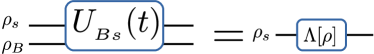
Figure 1: The reduced time evolution operator (CPTP map) on an ensemble of spins coupled to a bath.

For completeness we briefly describe how to connect these two descriptions. In a master equation, the relaxation operator $\hat{\Gamma}$ is induced by the bath coupling. The interaction Hamiltonian can be written as:

$$\mathcal{H}_{Bs}=\sum\limits_{i}B_{i}(t)\otimes A_{i}$$

where the operators $A_{i}$ are acting on the spin system and the operators $B_{i}(t)$ are fluctuating randomly and are acting on the bath system. One can find the bath time correlation function

$$R^{ij}(\tau)=\overline{B_{i}^{\dagger}(t)B_{j}(t-\tau)}$$ (5)

from which the spectral density of noise is known, $J^{ij}(\omega)=\int d\tau e^{i\omega t}R^{ij}(\tau)$. Then, under some assumptions (ErnstBook $\&$ OQSBook ), one can find the relaxation superoperator,

$$\hat{\Gamma}\ [\rho_{s}(t)]=\sum\limits_{i,j,\omega}J_{ij}(\omega)[A_{j}(\omega)\rho_{s}(t)A_{i}^{\dagger}(\omega)-A_{i}^{\dagger}(\omega)A_{j}(\omega)\rho_{s}(t)+h.c]$$

where $A(\omega)$ is the component of $A$ in the frequency domain. Given this last relation for $\hat{\Gamma}[\rho_{s}]$, the solution of the master equation in Eq.(4), is the same as the quantum evolution map defined in Eq.(II.1) under Markovian interaction.

II.2 Cavity Interaction

We can also find an effective map for the coupling of the spins to the cavity/coil, $\mathcal{H}_{c}$ and $\mathcal{H}_{sc}$. This system evolves unitarily

$$\rho_{sc}(t)=U_{sc}.(\rho_{s}\otimes|\psi\rangle_{c}\langle\psi|).U_{sc}^{\dagger}$$

where $U_{sc}=\exp(-i(\mathcal{H}_{c}+\mathcal{H}_{sc})\ t)$. For our analysis, the cavity does not distinguish between spins and the spins only couple to a single mode. This is described by the Tavis-Cumming Hamiltonian, (Tavis )

$$\mathcal{H}_{c}+\mathcal{H}_{sc}=\omega_{c}\ aa^{\dagger}+g\ J_{x}(a+a^{\dagger}).$$

Here $J_{x}=\sum\limits^{N}_{i=1}S^{(i)}_{x}$ is the x component of the total spin angular momentum, and $a$ and $a^{\dagger}$ are the ladder operators. According to this model, the detection coil does not distinguish spins and in a measurement, the net magnetization of the whole ensemble is recorded, given by $m=\sum\limits_{i=1}^{N}s^{(i)}$ with $s\in\{+\frac{1}{2},-\frac{1}{2}\}$. So, a measurement leaves the spin ensemble in a totally symmetric submanifold with net magnetization $m$. To see the effect of measurement explicitly, we note that the cavity is coupled to additional degrees of freedom that produce the observed measured outcomes (e.g, electronics). So effectively, the spin system couples to the measurement device ($c^{\prime}$) via the cavity interactions and once the measurement is completed the cavity is left in its initial state. This allows us to drop the cavity from the model. If the detection has an accuracy of one single spin flip, the possible measured outcomes are $m\in\{-\frac{N}{2},-\frac{N}{2}+1,...,\frac{N}{2}\}$ and correspondingly the measurement device Hilbert space is spanned by an orthonormal basis $\{|m\rangle\}$. For the evolved state $\rho_{sc^{\prime}}(t)$, tracing over the measurement device gives

$$Tr_{c^{\prime}}[\rho_{sc^{\prime}}(t)] = Tr_{c^{\prime}}[U_{sc^{\prime}}.(\rho_{s}(0)\otimes|\psi\rangle\langle\psi|{\color[rgb]{0,0,0})}.U_{sc^{\prime}}^{\dagger}]$$ (6)

$$\rho_{s}(t) = \sum\limits_{m}\langle m|U_{sc^{\prime}}|\psi\rangle.\rho_{s}(0).\langle m|U_{sc^{\prime}}|\psi\rangle^{\dagger}$$

$$= \sum\limits_{m}\mathcal{M}_{m}.\rho_{s}(0).\mathcal{M}_{m}^{\dagger}$$

where $\mathcal{M}_{m}=\langle m|U_{sc^{\prime}}|\psi\rangle$ is defined as the measurement operator assigned to the measurement outcome $m$. Here, the partial trace of any operator $\hat{O}$ is defined as $Tr_{B}[\hat{O}_{AB}]=\sum\limits_{b}(\mathbb{1}\otimes\langle b|)\hat{O}_{AB}(\mathbb{1}\otimes|b\rangle)$. According to Eq.(6), the effect of the interaction with the detection coil appears as an effective quantum map $\mathcal{E}[\rho]=\sum\limits_{m}\mathcal{M}_{m}.\rho_{s}.\mathcal{M}_{m}^{\dagger}$ on the spin ensemble. It is easy to check that $\mathcal{E}[\rho]$ is also a CPTP map and hence, $\sum\limits_{m}\mathcal{M}^{\dagger}_{m}\mathcal{M}_{m}=\mathbb{1}$.

Notice that we considered an initial pure state $|\psi\rangle$ for the measurement device. One can generalize this argument for any initial mixed state, $\rho_{c}(0)$, because it can be written as a convex combination of pure states and all of the maps in the presented model are linear.

In a quantum measurement there is a trade off between the amount of information obtained and the amount of disturbance introduced in the system. Say the detection coil measures the classical value $m_{0}$, then the spin ensemble’s state conditioned on the knowledge $m_{0}$ is updated to Nielson

$$\rho^{|m_{0}}=\frac{\mathcal{M}_{m_{0}}.\rho_{s}.\mathcal{M}_{m_{0}}^{\dagger}}{P(m_{0})}$$

where $P(m_{0})=Tr[\mathcal{M}^{\dagger}_{m_{0}}\mathcal{M}_{m_{0}}\rho_{s}]$ is the probability that such an event occurs.

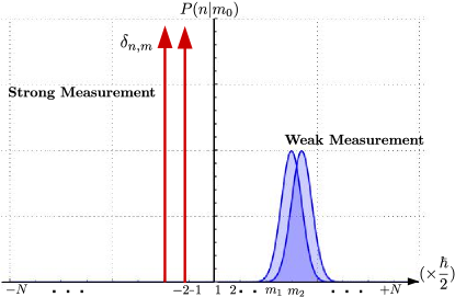
Figure 2: The conditional probability distribution of a strong measurement and a weak measurement are compared. In a strong measurement, the updated density matrix collapses sharply to the submanifold $m_{0}$ and this leads to a delta function distribution (red). Whereas, in a weak measurement, the density matrix is less disturbed and it collapses to an area centered at $m_{0}$. So, the corresponding probability distribution has a finite width (blue). The horizontal axis is in $\frac{\hbar}{2}$ unit and represents the net magnetization of the ensemble.

In the case of a strong measurement, the ensemble magnetization, $m_{0}$, is known with certainty. Therefore, the spin ensemble density matrix collapses (disturbance) to the $m=m_{0}$ manifold only, and if we make a second measurement immediately afterwards, the outcome $m_{0}$ is reproduced. In other words, the conditional probability distribution of the second measurement is a delta function, i.e, $P(n|m_{0})=\delta_{n,m_{0}}$. In the case of a weak measurement, the measurement apparatus is less precise and the spin ensemble state collapses not only to the $m=m_{0}$ manifold but also to the other neighboring manifolds, $n\neq m_{0}$. So, if we immediately make another measurement, the outcome $m_{0}$ may not be reproduced. In other words, the conditional probability distribution $P(n|m_{0})$ could be a distribution function with mean value $m_{0}$ and a width $w$ which is in inverse relation with the accuracy of the measurement device (Fig.2). We will provide a more detailed model of a strong and a weak measurement in sections III and IV.

II.3 N Spins Coupled to the Bath and the Cavity

So far, we have considered the effect of coupling to the measurement apparatus and the reduced quantum evolution map on the spin ensemble as two independent processes. However, in an NMR measurement these two processes occur simultaneously (Eq.1). So,

$$U_{Bsc}(T)=\mathcal{T}e^{-i\int_{0}^{T}\mathcal{H}_{tot}(t^{\prime})\ dt^{\prime}}.$$

The various contributions of $\mathcal{H}_{tot}$ do not in general commute at all times and so the formal solution is not practically helpful. One can discretize the total evolution time, $T=n\ t$, in which $t$ is small enough to allow a first order approximation. Then, for a short time evolution $t$, the first order of the Magnus expansion (Waugh ) is

$$U_{Bsc}(t) \approx e^{-i\int_{0}^{t}(\mathcal{H}_{s}+\mathcal{H}_{B}+\mathcal{H}_{Bs}(t^{\prime}))dt}e^{-i(\mathcal{H}_{c}+\mathcal{H}_{sc})t}$$

$$= U_{sc}(t)U_{Bs}(t)$$

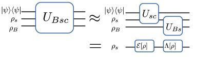
Figure 3: A first order approximation of time evolution of a bath-spin ensemble-cavity system is presented.

For example, in the case of $\mathcal{H}_{s}=\omega_{0}J_{z}$ and the Tavis-cumming model for interaction with the cavity, this approximation is valid if $t\ll\frac{1}{\sqrt{\omega_{0}g}}$. In this first order approximation, the effective quantum evolution map for the short time period $t$ on the spin ensemble is:

$$\rho_{s}(t) = \hat{\mathcal{S}}_{t}[\rho_{s}]$$

$$= Tr_{Bc}[U_{Bsc}.\rho_{Bsc}(0).U_{Bsc}^{\dagger}]$$

$$\approx Tr_{Bc}[(U_{Bs}.U_{sc}).\rho_{Bsc}(0).(U_{Bs}.U_{sc})^{\dagger}]$$

$$= \Lambda[\mathcal{E}[\rho_{s}(0)]]$$

where $\rho_{Bsc}(0)=\rho_{B}(0)\otimes\rho_{s}(0)\otimes|\psi\rangle\langle\psi|$. Therefore, a quantum evolution map on the spin ensemble, $\hat{\mathcal{S}_{T}}$, can be approximated by a sequence of measurement-evolution processes as schematically is shown in Fig.4.

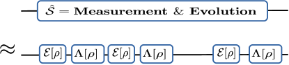
Figure 4: The effective time evolution operator $\hat{\mathcal{S}}$ on a spin ensemble is approximated by a sequence of measurement-evolution processes.

In the following sections, we apply this model to the examples of both strong and weak measurements under the evolution of a collective depolarizing map or any arbitrary CPTP map on individual spins. In each cases, we find the spin noise and its correlation function.

III Strong Measurement Model

Suppose we have $N$ identical spin half particles and we have no information about their spin orientation. So, at $t=0$, the density matrix $\rho_{0}=\frac{\mathbb{1}}{2^{N}}$ describes “our knowledge” about the system which is maximal ignorance. Now, according to the model presented in previous section, we make a series of strong measurements on the system by which we obtain information about the collective magnetization, M. Between two subsequent measurements, there is a time interval $\delta t$ during which the system evolves under a quantum evolution map $\Lambda_{\delta t}$. Without loss of generality, we assume the collective measurements are along the z axis. Of course, NMR detection is in the $x-y$ plane, but, for this analysis the direction is of no importance. At $t=t_{n}$, the recorded data, $\textbf{M}(t_{n})$, are eigenvalues of the z component of the total spin angular momentum, $\textbf{J}_{z}=\sum\limits^{N}_{i=1}\ S^{(i)}_{z}$. This choice of collective measurement is not the common one in NMR, usually $N\langle S_{z}\rangle$ is used as the ensemble signal. However, in order to see the spin noise effects, one needs to keep track of what has been learned about the ensemble in each measurement rather than just the mean value. Therefore we do the analysis in the total angular momentum space. This has been used before Poulin .

The action of a strong measurement is described by a set of projection valued measure (PVM) operators, which we denoted as ${\color[rgb]{0,0,0}\{\mathcal{M}_{m}=}\Pi_{m}\}$ and are given by

$$\textbf{J}_{z} = \sum\limits_{m}m\ \Pi_{m}$$ (9)

$$\Pi_{m} \equiv \sum_{j=|m|}^{N/2}\sum_{a=1}^{A_{j}}\ |j,m,a\rangle\langle j,m,a|.$$

where $\hbar=1$. Here, $|j,m,a\rangle$ are degenerate eigenstates of the total spin angular momentum $\vec{J}=\sum\limits_{i=1}^{N}\vec{S}^{(i)}$ as well as its z component $\textbf{J}_{z}$ operator. For $N$ spin half particles, $j=j_{0},j_{0}+1,...,N/2$ where $j_{0}=0\ (1/2)$ if N is even (odd). For each total spin angular momentum’s eigenvalue, $j$, the collective magnetization in the z direction is $m=-j,j+1,...,j$, and, the state degeneracy label is $a=1,2,...,A_{j}$ where $A_{j}=\left(\begin{array}[]{c}N\\ \frac{N}{2}+j\end{array}\right)-\left(\begin{array}[]{c}N\\ \frac{N}{2}+j+1\end{array}\right)$[18]. These eigenstates span the whole Hilbert space and form a basis for an ensemble of spins. It is common to consider $j$ as the principle quantum number and, $m$ as the second quantum number. However, mathematically it is equivalent to consider $m$ as the principle number, $m\in\{-N/2,-N/2+1,...,N/2\}$ and $|m|\leq j\leq N/2$ as the second quantum number which is the case in our notation. Note, by this definition, $\{\Pi_{m}\}$ satisfies the conditions of Projective Value Measure (PVM) operators, i.e, $\Pi_{m}.\Pi_{n}=\delta_{mn}\Pi_{m}$ and $\sum\limits_{m}\Pi_{m}=\mathbb{1}$. An example of a strong measurement on a single spin is Stern-Gerlach experiment where the measurement operators are $\Pi_{+}=|\uparrow\rangle\langle\uparrow|$ and $\Pi_{-}=|\downarrow\rangle\langle\downarrow|$ which are orthogonal projective operators corresponding to the outcome “up” and “down”. Here, $\Pi_{m}$ are the generalized form for an $N$ spin projective measurement when the detection coil has the precision of one single spin.

The first measurement at $t_{1}$, results in outcome $m_{1}\in[-\frac{N}{2},\frac{N}{2}]$ which occurs with probability $P(m_{1};t_{1})$. This probability is a binomial (semi-Gaussian) distribution with zero mean and $\sqrt{N}$ standard deviation, because

$$P(m_{1};t_{1}) = Tr[\Pi_{m_{1}}.\rho_{0}]=\frac{Tr[\Pi_{m_{1}}]}{2^{N}}$$ (10)

$$E[\textbf{M};t_{1}] = Tr[J_{z}.\rho_{0}]=0$$

$$\sigma[\textbf{M};t_{1}] = \sqrt{Tr[J_{z}^{2}.\rho_{0}]-(Tr[J_{z}.\rho_{0}])^{2}}=\frac{1}{2}\sqrt{N}$$

This result matches what we intuitively expect. Each spin has magnetization $s_{i}\in\{+\frac{1}{2},-\frac{1}{2}\}$, and, in each measurement shot, we take $N$ samples from a distribution $P(s)$ with a width of $\frac{1}{2}$. Therefore, according to the central limit theorem, the collective magnetization $m=\sum^{N}\limits_{i=1}s_{i}$ itself is a random variable whose distribution is Gaussian with width of $\frac{\sqrt{N}}{2}$. Because the spins are indistinguishable, $Tr[\Pi_{m}]$ counts the number of configurations that all result in $m$ net magnetization and therefore $P(\textbf{M};t_{1})$ is a binomial distribution.

Once we learn the system, we must update its density matrix according to “our knowledge” of the outcome. So, given the outcome $m_{1}$, the state update rule Nielson dictates that

$$\rho^{|\textbf{M}=m_{1}}=\frac{\Pi_{m_{1}}.\rho_{0}.\Pi_{m_{1}}}{P(m_{1};t_{1})}=\frac{\Pi_{m_{1}}}{Tr[\Pi_{m_{1}}]}.$$ (11)

The state (11) evolves under a quantum map $\Lambda$ during the time interval $\delta t$ after which the next measurement takes place. As an example, we consider a collective depolarizing map where with probability $(1-\lambda)=\text{exp}[-\delta t/T]$ the quantum state is preserved and with probability $\lambda$ it turns to a fully mixed state. The characteristic time $T$ is a function of the depolarizing strength. Physically, a depolarizing map could be a result of a relaxation process in the system and mathematically is given by

$$\Lambda[\rho]=(1-\lambda)\ \rho+\lambda\ \frac{\mathbb{1}}{2^{N}}.$$ (12)

Now, in the second step, the evolved state $\Lambda[\rho^{|m_{1}}]$ is measured and outcome $m_{2}$ is obtained whose probability is given by $P(m_{2};t_{2}|m_{1})=(1-\lambda)\ \delta_{m_{1},m_{2}}+\lambda\ P(m_{2};t_{1})$. This $P(\textbf{M};t_{2}|m_{1})$ will be again a semi-Gaussian distribution with a conditional mean and conditional standard deviation

$$E(\textbf{M};t_{2}|m_{1}) = (1-\lambda)\ m_{1}$$ (13)

$$\sigma(\textbf{M};t_{2}|m_{1}) = \sqrt{\lambda\ (\frac{N}{4}+(1-\lambda)\ m^{2}_{1})}$$

Thus, the second measurement statistics are correlated with the first measurement outcome $m_{1}$. This correlation does not last forever and is limited by the relaxation time of the dissipative system, $T$. For instance, if we record data so slowly, $\delta t>>T$( or $\lambda\rightarrow 1$), each measurement data $m_{k}$ is sampled from a fixed distribution $P(\textbf{M};t_{1})$ with zero mean and $\frac{1}{2}\sqrt{N}$ standard deviation and there will be no correlation between data, Eq.(13). In another extreme case, when we record data quickly, $\delta t<<T$, then $1-\lambda\approx 1-\frac{\delta t}{T}$ and the system does not evolve, hence, the data is repeatable, which is a property of a projective measurement. In non-extreme regimes, when $\delta t<T$, the data is sampled from semi- binomial distributions whose mean and variance are fluctuating from one measurement to another.

After a long data acquisition a list of outcomes $\{m_{1},m_{2},....,m_{k}\}$ is obtained which constructs the spin noise signal. The spin noise is the net magnetization of an ensemble whose fluctuating value is bounded by $\frac{N}{2}$ and -$\frac{N}{2}$. At step $k$th, $m_{k}$ is a random variable sampled from semi-Gaussian distribution $P(\textbf{M};t_{k}|m_{k-1},...,m_{2},m_{1})$ whose mean and variance are correlated with previous recorded data. For the particular choice of a depolarizing map, using inductive reasoning, we obtain that the the joint probability distribution between any two data points is

$$P(m_{i};t_{i},m_{j};t_{j}) = (1-\lambda)^{i-j}\ \delta_{m_{i},m_{j}}\ P(m_{j};t_{j})$$

$$+ \eta_{i-j}\ P(m_{i};t_{i})\ P(m_{j};t_{j})$$

where $\eta_{k}=\lambda+(1-\lambda)\ \eta_{k-1}$ and $\eta_{0}=0$ and $P(m;t_{i})=P(m;t_{1})=Tr[\Pi_{m}.\rho_{0}]$. Relation.(III) indicates that, with the probability of $(1-\lambda)^{k}\sim e^{-t_{k}/T}$, the two measurements separated by $t_{k}=k\ \delta t$, are perfectly correlated and with the probability of $\eta_{k}$, they are two independent random variables. In other words, the closer the two measurements are in time, the more likely that their distributions are correlated. Given Eq.(III), one can compute the covariance function as a measure of the correlation,

$$R(k) \equiv E(\textbf{M};t_{k+i},\textbf{M},t_{i})-E(\textbf{M};t_{k+i})E(\textbf{M},t_{i})$$ (15)

$$= \frac{N}{4}\ e^{-t_{k}/T}$$

where the expectation values are calculated using $E(X;t_{1})=\sum_{x}x\ P(x;t_{1})$ and $E(X;t_{i},Y;t_{j})=\sum_{x,y}x\ y\ P(x;t_{i},y,t_{j})$ and we assumed an initially fully mixed state.

This analysis has considered a collective evolution $\Lambda$ and a collective measurement $\Pi_{m}$ over an ensemble where the collective measurement preserves coherences within the subspace $m$.

III.1 Arbitrary Quantum Map $\Lambda$ for non-interacting spins

We can further generalize the description by extending it to any arbitrary CPTP quantum map acting on individual spins. More precisely, suppose the spins are not interacting with each other, that there is no field inhomogeneity and also no variation of the $B_{1}$ field, and, that each individual spin interacts with its own bath. Therefore, spins are indistinguishable to the environment and one can model the ensemble quantum evolution as $\Lambda=\Phi^{\otimes N}$ where $\Phi$ is a CPTP map on a single spin. In this picture, each spin is an open quantum system.

As before, consider a totally mixed initial state for each spin, $\rho_{0}=(\frac{\mathbb{1}}{2})^{\otimes N}$, and make a strong measurement along the z axis. Upon the measurement with outcome $m$, there are $\frac{N}{2}+m$ number of spins with up orientation and $\frac{N}{2}-m$ with down orientation. So, the measurement statistics are given by

$$P(m;t_{1}) = \left(\begin{array}[]{c}N\\ \frac{N}{2}+m\end{array}\right)(\frac{1}{2})^{\frac{N}{2}+m}(\frac{1}{2})^{\frac{N}{2}-m}.$$ (18)

The PVM operator given in Eq.(1) can also be expanded in the tensor product basis as:

$$\Pi_{m}=\sum\limits_{p}\hat{\mathcal{P}}_{p}[|\uparrow\rangle\langle\uparrow|^{\otimes\frac{N}{2}+m}\otimes|\downarrow\rangle\langle\downarrow|^{\otimes\frac{N}{2}-m}].$$

Here, since the spins are indistinguishable, there is a sum over all possible spin permutations that results in net spin magnetization $m$. So, $p\in\{1,...,\left(\begin{array}[]{c}N\\ \frac{N}{2}+m\end{array}\right)\}$. Upon recording the classical value $m_{1}$, the density matrix is updated to

$$\rho^{|m_{1}} = \frac{\Pi_{m_{1}}.\rho_{0}.\Pi_{m_{1}}}{P(m_{1};t_{1})}$$

$$= \frac{\sum\limits_{s}\hat{\mathcal{P}}_{s}[|\uparrow\rangle\langle\uparrow|^{\otimes\frac{N}{2}+m_{1}}\otimes|\downarrow\rangle\langle\downarrow|^{\otimes\frac{N}{2}-m_{1}}]}{2^{N}P(m_{1};t_{1})}.$$

This updated state evolves under $\Lambda$ which means that each spin evolves under $\Phi$. An example of a single qubit CPTP map $\Phi$ would be a rotation around axis $\hat{r}_{1}$, a relaxation around axis $\hat{r}_{2}$ and a dephasing around axis $\hat{r}_{3}$ on the Bloch sphere. In general, the action of a map $\Phi$ on the spin basis can be written as

$$\Phi[|\uparrow\rangle\langle\uparrow|]=(1-\alpha)\ |\uparrow\rangle\langle\uparrow|+\alpha\ |\downarrow\rangle\langle\downarrow|+\text{Off diagonal}$$

$$\Phi[|\downarrow\rangle\langle\downarrow|]=(1-\beta)\ |\downarrow\rangle\langle\downarrow|+\beta\ |\uparrow\rangle\langle\uparrow|+\text{Off diagonal}$$

where $\alpha$ and $\beta$ are variables which are determined by the map’s parameters such as evolution time $\delta t$, frequency $\omega$, relaxation and dephasing rates and the directions $\hat{r}_{1},\hat{r}_{2},\hat{r}_{3}$.

The second measurement on $\Lambda[\rho^{|m_{1}}]$ results in outcome $m_{2}$ which occurs with probability

$$P(m_{2};t_{2}|m_{1})=\sum^{\frac{N}{2}+m_{1}}\limits_{k=0}\sum^{\frac{N}{2}-m_{1}}\limits_{l=0} \{\text{Bin}(\frac{N}{2}+m_{1},k,\alpha)$$

$$\text{Bin}(\frac{N}{2}-m_{1},l,\beta)\delta_{{}_{m_{2}-m_{1},l-k}}\}$$

where $\text{Bin}(n,k,p)=\left(\begin{array}[]{c}n\\ k\end{array}\right)p^{k}(1-p)^{n-k}$. This new distribution is again a binomial with mean value

$$E(\mathbb{M},t_{2}|m_{1})=m_{1}(1-(\alpha+\beta))+(\frac{N}{2})(\alpha-\beta)$$

and standard deviation

$$\sigma(\textbf{M};t_{2}|m_{1}) = \sqrt{\frac{N}{2}(\alpha(1-\alpha)+\beta(1-\beta)}$$

$$+ \sqrt{m_{1}(\alpha(1-\alpha)-\beta(1-\beta)}.$$

As the above relations indicate, depending on the evolution map’s parameters, $\alpha$ and $\beta$, the statistics of the noise are different. Nevertheless, the spin noise magnitude still scales with $\sqrt{N}$ and exhibits a time correlation. Notice, it is not necessary to consider an open system interacting with an environment to see the spin fluctuation. For example, even in the case of simple unitary evolution where $\alpha=\beta=\sin^{2}[\omega\ \delta t]$, these correlated fluctuations exist.

In order to find the correlation function, we need to know the joint probability distribution, Eq.(15). In the particular choice of a totally mixed input state, after each measurement, the updated density matrix is $\Pi_{m_{k}}/Tr[\Pi_{m_{k}}]$. Therefore, $P(m_{k};t_{k}|m_{{\color[rgb]{0,0,0}k}-1})=P(m_{2};t_{2}|m_{1})$ for all $t_{k}$, and hence, the joint probability distribution of any two data points is:

$$P(m_{i};t_{i},\ m_{j};t_{j}) = \sum\limits_{l_{i-j},...,l_{i-1}}P(m_{i};t_{i}|l_{i-1})$$

$$\times...\times\ P(l_{i-j};t_{i-j}|m_{j})P(m_{j};t_{j}).$$

Substituting Eq.(III.1) into relation (III.1) gives us an analytic expression for the joint probability distribution and in the large ensemble limit and for the totally mixed input state, one can approximate each $P(m_{k},t_{k}|m_{k-1})$ with a Gaussian distribution whose mean and variance are fluctuating from one measurement to the next.

III.1.1 Arbitrary Initial State

In this section, we consider $N$ identical and non interacting spins, $\rho_{0}=\varrho^{\otimes N}$ where $\varrho$ is an arbitrary single spin density matrix that is expanded as:

$$\varrho=a\ |\uparrow\rangle\langle\uparrow|+(1-a)\ |\downarrow\rangle\langle\downarrow|+b\ |\uparrow\rangle\langle\downarrow|+b^{*}\ |\downarrow\rangle\langle\uparrow|.$$ (22)

The first measurement on this ensemble results in the statistical distribution

$$P(m_{1};t_{1}) = \left(\begin{array}[]{c}N\\ \frac{N}{2}+m\end{array}\right)(a)^{\frac{N}{2}+m_{1}}(1-a)^{\frac{N}{2}-m_{1}}.$$ (25)

This distribution does not distinguish $\varrho$ from a diagonal state $\tilde{\varrho}=a\ |\uparrow\rangle\langle\uparrow|+(1-a)\ |\downarrow\rangle\langle\downarrow|$ since the measurement is along the z axis. Therefore, it is sufficient to consider $\tilde{\varrho}$ as an arbitrary initial state. Upon the strong measurement given by $\Pi_{m}$, the state update rule implies that

$$\rho^{|m_{1}} = \sum\limits_{s}(a)^{\frac{N}{2}+m_{1}}(1-a)^{\frac{N}{2}-m_{1}}$$

$$\times \frac{\hat{\mathcal{P}}_{s}[|\uparrow\rangle\langle\uparrow|^{\otimes\frac{N}{2}+m_{1}}\otimes|\downarrow\rangle\langle\downarrow|^{\otimes\frac{N}{2}-m_{1}}]}{P(m_{1};t_{1})}.$$

By replacing $P(m_{1};t_{1})$ with Eq.25, we see that the above state is identical to the updated state (III.1) where the experiment started from a mixed state. Despite the fact that the first measurement statistics differentiate an arbitrary initial state ($\varrho$ or $\tilde{\varrho}$) from an identity state ($\mathbb{1}/2^{N}$), their corresponding updated states are no longer distinguishable to the subsequent measurement-evolution processes. As a result, except for the first data point, the statistical fluctuations of spin noise are the same whether we start from a mixed state or from an arbitrary initial state.

IV Weak Measurement Model

In an NMR measurement, it is too idealistic to assume that the detection process can resolve a single spin. If we relax this assumption, the projective measurement operators, $\mathcal{M}_{m}=\Pi_{m}$, no longer describe the action of a measurement. One needs to assign a width of precision to the measurement apparatus which results in an overlap between the different subspaces (Fig.2). Therefore, once the data $m_{0}$ is recorded, the spin ensemble density matrix collapses not only to the $m_{0}$ subspace but also to other subspaces with $l\neq m_{0}$. The most general type of measurement are mathematically modeled by positive valued operator measure (POVM) operators, $E_{m}$, which result in measurement statistics $P(m)=Tr[E_{m}\rho]$, Nielson . A PVM is a special case of this. Therefore, we adapt the spin noise model by relaxing the assumption of a strong measurement to a weak measurement and defining POVM elements, $E_{m}=\mathcal{M}_{m}^{\dagger}\mathcal{M}_{m}$, as a sum of PVM operators,

$$E_{m}=\sum\limits^{N/2}_{l=-N/2}D(m,l)\ \Pi_{l}$$ (27)

where $D(m,l)$ is a two variable function whose form is limited by physical constraints:

1. The measurement is trace preserving. So,

   $$\sum\limits_{m}E_{m}=\mathbb{1}\ \Rightarrow\ \mbox{ for each}\ l\hskip 7.11317pt\sum_{m}D(m,l)=1.$$

   This means that $D$ is certainly a distribution relative to $m$, but it does not have to be a distribution relative to $l$. This condition becomes particularly important when we get close to the boundaries $\pm\frac{N}{2}$.
   
   

2. Since the detector records data $m$ as the outcome, we expect $D$ to have its maximum value at $l=m$. So,

   $$\max\limits_{l}D(m,l)=D(m,m).$$

   
   
   

3. In a weak measurement, the measurement outcome is less reliable; if the measurement apparatus records $m$, there is a probability $D(m,l)$ that the updated system collapses to other subspaces with $l\neq m$. One expects the further apart $l$ and $m$ are, the less likely it is to collapse into the $l$ subspace. Thus, $D(m,l)$ should decrease as $|l-m|$ increases and its width should be inversely propotioned to the reliability of the measurement device, $1/w$.
   
   

4. $D$ need not be a symmetric function. For instance, we know it must be a distribution relative to $m$ but it need not have restriction relative to $l$. So, in general $D(a,b)\neq D(b,a)$.
   
   

Considering the above constraints, we model the function $D(m,l)$ by a semi-Gaussian distribution:

$$D(m,l)=A_{l}\ e^{\frac{-(m-l)^{2}}{2w^{2}}}\mbox{ where}\ A_{l}=(1/\sum\limits_{k}e^{\frac{-(k-l)^{2}}{2w^{2}}}).$$ (28)

In this model, we quantify the “weakness” of the measurement by the quantity $w$. In the extreme limit of a “strong” measurement, when $w\rightarrow 0$, $D$ becomes sharp, $D(m,l)\rightarrow\delta(m-l)$, and hence, $E_{m}=\Pi_{m}$ (Fig.2). In the limit of a “very weak” measurement when $w\rightarrow\infty$, $D(m,l)$ becomes a uniform distribution and hence $E_{m}\propto\mathbb{1}$, and so, the state $\rho_{0}$ is not affected by the state update rule. In other words, the weakest measurement causes the least disturbance to the system.

Consider an $\epsilon$-polarizing quantum map, $\Lambda[\rho]=(1-\lambda)\ \rho+\lambda\ \rho_{0}$, for the evolution process which tends to return the state to the thermal equilibrium polarization with $Tr[\textbf{J}_{z}.\rho_{0}]=\epsilon$. As an example, consider the initial state $\rho_{0}=\sum\limits_{k}q_{0}(k)\ \frac{\Pi_{k}}{Tr[\Pi_{k}]}$ in which $q_{0}(k)$ is a density function with mean value $\epsilon=\sum\limits_{k}k\ q_{0}(k)$. For instance, in the case of a mixed state, $\rho_{0}=\frac{\mathbb{1}}{2^{N}}$, $q_{0}(k)=Tr[\Pi_{k}]/2^{N}$ is a binomial distribution with zero mean. Given $\rho_{0}$, the first weak measurement results in $m_{1}$ with a probability

$$P(m_{1};t_{1}) = Tr[E_{m_{1}}.\rho_{0}]$$

$$= \sum\limits_{k}D(m_{1},k)\ q_{0}(k).$$

It is known that given the distribution, $P(m)$, the updated density matrix is not uniquely determined in case of a weak measurement, Nielson . This is because, the set of $\{\mathcal{M}_{m}\}$ that satisfies $\mathcal{M}_{m}^{\dagger}\mathcal{M}_{m}=E_{m}$ is not unique. Nevertheless, one of the possible ways of updating the density matrix is $\mathcal{M}_{m}=\sqrt{E_{m}}$ , which gives

$$\rho^{|m_{1}} = \frac{\sqrt{E_{m_{1}}}.\rho_{0}.\sqrt{E_{m_{1}}}}{P(m_{1};t_{1})}$$

$$= \sum\limits_{k}q_{1}(k|m_{1})\frac{\Pi_{k}}{Tr[\Pi_{k}]}.$$

Here we define $q_{1}(k|m_{1}):=\frac{D(m_{1},k)\ q_{0}(k)}{P(m_{1};t_{1})}$ to be the updated density function. As desired, the updated density matrix collapses not only to $\frac{\Pi_{m}}{Tr[\Pi_{m}]}$ but also to other neighboring subspaces, $k\neq m_{1}$, and its range depends on the measurement “weakness” $w$. This semi-localized state around $m_{1}$, will then evolve under the $\epsilon$-polarizing map, $\Lambda$. Similar to the PVM case, by performing the second measurement, we obtain a conditional distribution

$$P(m_{2};t_{2}|m_{1}) = Tr[E_{m_{2}}.\Lambda[\rho^{|m_{1}}]]$$

$$= (1-\lambda)\ \sum\limits_{k}D(m_{2},k)\ q_{1}\ (k|m_{1})$$

$$+ \lambda\ \sum\limits_{k}D(m_{2},k)q_{0}(k).$$

The fact that the overlap between $D(m_{2},l)$ and $D(m_{1},l)$ appears in the first term of the last equation confirms that, as long as $\lambda\neq 1$ and $w\neq\infty$, there are correlations carrying on from one measurement to another.

We calculated the joint probability distribution between any two data points and obtained

$$P(m_{i};t_{i},m_{j};t_{j}) = (1-\lambda)^{i-j}\sum\limits_{l}D(m_{i},l)\ D(m_{j},l)\ q_{0}(l)$$

$$+ \eta_{i-j}\ P(m_{i};t_{i})\ \ P(m_{j};t_{j}).$$

Despite the fact that a strong and a weak measurement result in different statistical distributions, ( i.e. $Tr[\Pi_{m}\rho]\neq Tr[E_{m}\rho]$) there are common features in both limits, most importantly, the statistics of instances are correlated with previous data. These correlations are a result of the quantum evolution map between measurements.

Thus far, we have not included the suggested Gaussian model for $D(m,l)$. If we do so, the covariance function becomes

$$R(k)=\frac{N}{4}\ (1-\lambda)^{k}+(\eta_{k}-1)\ E(\textbf{M};t_{1})^{2}.$$ (30)

One can test this relation for a totally mixed input state and reproduce the exact result in Eq.(15). This indicates that spin fluctuations have a similar behavior in both the strong and the weak measurement limit.

V Conclusion

An open quantum system model of the spin noise signal in NMR was described. We have shown that the inherent spin fluctuations can be described by the nature of quantum measurements, the state update rule and quantum evolution. We analyzed our model for arbitrary initial states including the identity, as well as any arbitrary quantum evolution CPTP map acting on non-interacting spins, with the depolarizing map as an example of a collective quantum evolution. We calculated the joint probability distribution and the covariance function for different examples in both the limits of strong and weak measurement.

The proposed spin noise model predicts the statistical fluctuation of a spin ensemble by considering a collective measurement and a collective quantum evolution while retaining the average properties such as thermal polarization. Previous computational models of spin noise have introduced a fluctuating field over the ensemble to create dephasing and account for noise correlations (QuantumOrigin ). Here, the model does not require such a field, the fluctuations are a function of the update rule that propagates over knowledge of the system. This analysis is intended to illustrate that with a description of the spin, the cavity and the bath interactions one may straightforwardly calculate the properties of spin noise, including its correlation function. Such descriptions are useful in analyzing experimental instances of spin noise, in particular, with the development of spin based quantum information processors that have long lived spin states and small number of spins.

The authors thank O. Moussa and M. Mirkamali for helpful discussions. We acknowledge support from Industry Canada, CERC, NSERC, CIFAR and Province of Ontario.

Appendix A

In this appendix, we give a concrete example of a spin noise model. Consider $100$ spin half particles each oriented randomly in the Bloch sphere, $\rho_{0}=(\frac{\mathbb{1}}{2})^{\otimes N}$. At $t=t_{1}$ we measure the magnetization along the $z$ axis, so, the measured value $m$, is the z component of the ensemble’s magnetization, i.e, $m=\sum\limits_{i=1}^{100}s_{i}$ with $s_{i}=\pm\frac{1}{2}$. Thus, $m\in\{-50,-49,...,0,...,49,50\}$ is a random number sampled from the probability distribution $P(\textbf{M};t_{1})$. In this example,

$$P_{str}(\textbf{M};t_{1}) = Tr[\Pi_{\textbf{M}}.\rho_{0}]=\text{Bin}(N,\frac{N}{2}+\textbf{M},\frac{1}{2}),$$ (31)

$$P_{wk}(\textbf{M};t_{1}) = Tr[E_{\textbf{M}}.\rho_{0}]=\sum\limits_{k=-\frac{N}{2}}^{\frac{N}{2}}D(\textbf{M},k)$$

$$\hskip 56.9055pt\times\text{Bin}(N,\frac{N}{2}+k,\frac{1}{2}).$$

where the subscript $st$ (or $wk$) refers to the strong (or the weak) measurement. If one repeats this first measurement with the same initial state, $\rho_{0}$, many times, a statistical distribution of $\textbf{M}(t_{1})$ will be obtained. We implemented this numerically and the results are shown in Fig.5.

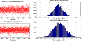
Figure 5: 3000 identical measurements are performed on 3000 identically prepared spin states with $\rho_{0}=(\frac{\mathbb{1}}{2})^{\otimes N}$. Each data point is a random number $m_{1}$ sampled from the statistical distribution $P(\textbf{M};t_{1})$. A numerical estimation of $P(\textbf{M};t_{1})$ is computed and plotted on the right side for both strong and weak measurements. $N=100$ and $w=5$.

Once the data $m_{1}$ is recorded, the ensemble’s density matrix is updated to $\rho^{|m_{1}}=\frac{\Pi_{m1}}{2^{N}P_{st}(m_{1};t_{1})}$ or $\rho^{|m_{1}}=\frac{E_{m1}}{2^{N}P_{wk}(m_{1};t_{1})}$ depending on whether the measurement was strong or a weak. Now, we let the spin system evolves for certain time $\delta t$ under the following quantum evolution map,

$$\Lambda[\rho] = \Phi^{\otimes N}[\rho]\hskip 14.22636pt\text{where}$$ (32)

$$\Phi[\varrho] = (1-\lambda)U.\mathcal{\varrho}.U^{\dagger}+\lambda\frac{\mathbb{1}}{2}.$$

The CPTP map $\Phi$ acts on individual spins and for this example, we chose it to be a depolarizing map (relaxation) followed by a unitary rotation around the $x$ axis, i.e, $U=e^{-i\omega S_{x}\delta t}$. $\Phi$ is parametrized by $\lambda=1-e^{-\delta t/T}$ and $\theta=\omega\ \delta t$. Following the discussion in section.III.1, the probability of spin flip is $\alpha=\beta=(1-\lambda)(\sin\theta)^{2}+\frac{\lambda}{2}$. Following the spin noise model, once the system is measured and evolves under $\Lambda$, the second measurement is performed at $t=t_{2}$. The second measured outcome $m_{2}\in\{-50,-49,...,0,...,49,50\}$ is again a random number sampled from the conditional probability distribution $P(\textbf{M};t_{2}|m_{1})$. For this particular example, we computed the conditional probability distribution in the case of the strong measurement,

$$P_{st}(\textbf{M};t_{2}|m_{1}) = Tr[\Pi_{\textbf{M}}.\Lambda[\rho^{|m_{1}}]]$$

$$= \sum\limits_{i=0}^{\frac{N}{2}+m_{1}}\text{Bin}(\frac{N}{2}+m_{1},i,\alpha)$$

$$\times \text{Bin}(\frac{N}{2}-m_{1},\textbf{M}-m_{1}+i,\alpha)$$

as well as for the weak measurement,

$$P_{wk}(\textbf{M};t_{2}|m_{1}) = Tr[E_{\textbf{M}}.\Lambda[\rho^{|m_{1}}]]$$

$$= \sum\limits_{k,k^{\prime}=-\frac{N}{2}}^{\frac{N}{2}}D(\textbf{M},k)D(m_{1},k^{\prime})\text{Bin}(N,\frac{N}{2}+k^{\prime},1/2)$$

$$\times \frac{P_{st}(k;t_{2}|k^{\prime})}{P_{wk}(m_{1};t_{1})}$$

For the numerical simulation, we prepared identical initial states $\rho_{0}$, performed the first measurement on them, then post selected on that data with magnetization value, $\textbf{M}=m_{1}$. Given, these selected conditional states, $\Lambda[\rho^{|m_{1}}]$, we made a second measurement and recorded the data and its statistics as shown in Fig.6.

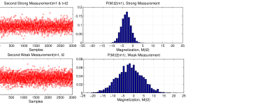
Figure 6: The raw data (left) and its corresponding statistical distribution (right) of the second measurement is presented for both cases of the strong and the weak measurements. Here, $\lambda=0.1$ and a small unitary rotation, $\theta=\pi/32$, are considered.

To see the correlation between the two subsequent data points, we plot the joint probability distribution $P(\textbf{M}_{2},\textbf{M}_{1})=P(\textbf{M}_{2}|\textbf{M}_{1})P(\textbf{M}_{1})$ where $\textbf{M}_{i}=\textbf{M}(t_{i})$. As shown in Fig.7, for the case of $\lambda=0$, $\theta=0$ (no evolution) and strong measurement, there is a maximum correlation between the two data points.

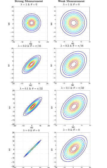
Figure 7: Contour plots of the joint probability distribution, $P(\textbf{M}_{2},\textbf{M}_{1})$ for different values of $\lambda$ and $\theta$. The top figure $\lambda=1$ and $\theta=0$, shows no correlation between subsequent data points and the bottom figure $\lambda=0$ and $\theta=0$ shows a maximum correlation between them.

But, for the case of weak measurement, there is less correlation even in the absence of any evolution. This shows that the data may not be reproducible in the case of a weak measurement. As the spin flip probability, $\alpha$, becomes larger (longer evolution), the two data points become less and less correlated as seen in Fig.7.

Measurement of subsequent data points proceeds in exactly the same style and the correlation function neighboring points does not change. Correlations are observed in all of these cases with the weak measurement data having less correlation than the strong.

References

- (1) F. Bloch, “Nuclear Induction”, Phys. Rev. 70, 460–474 (1946).
- (2) T. Sleator, E. L. Hahn, C. Hilbert and J. Clarke, “Nuclear Spin Noise” Phys. Rev. Lett. 55, 1742–1745(1985-1987).
- (3) M. A. McCoy and R. R. Ernst, “Nuclear Spin Noise at Room Temperature” Chem. Phys. Lett. 159, 587–593(1989).
- (4) M. Gueron and. J. L. Leroy, “NMR of water protons. The detection of their nuclear-spin noise, and a simple determination of absolute probe sensitivity based on radiation damping”, J. Magn. Reson. 85, 209–215 (1989).
- (5) H. J. Mamin, R. Budakian, B.W. Chui, and D. Rugar, “Detection and Manipulation of Statistical Polarization in Small Spin Ensembles”, Phys. Rev. Lett 91 (2003).
- (6) C. L. Degen, M. Poggio, H. J. Mamin and D. Rugar, “Role of Spin Noise in the Detection of Nanoscale Ensembles of Nuclear Spins”,Phys. Rev. Lett 99, 250601 (2007).
- (7) C. A. Meriles, L. Jiang, G. Goldstein, J. S. Hodges, J. Maze, M. D. Lukin and P. Cappellaro, “Imaging mesoscopic nuclear spin noise with a diamond magnetometer”, J. Chem. Phys. 133, 124105 (2010).
- (8) J. M. Nichol, T. R. Naibert, E. R. Hemesath, L. J. Lauhon, and R. Budakian, “Nanoscale Fourier-Transform Magnetic Resonance Imaging”, Physical Review X. 3, 031016 (2013).
- (9) N. Muller and A. Jerschow, “Nuclear Spin Noise Imaging”, PNAS vol. 103-no. 18-6790–6792 (2006).
- (10) D. I. Houllt and N. S. Ginsberg, “The quantum origin of the free induction decay signal and spin noise”, Journal of Magnetic Resonance 148, 182–199 (2001).
- (11) J. Tropp, “A quantum description of radiation damping and the free induction signal in magnetic resonance”, J. Chem. Phys. 139, 014105 (2013).
- (12) R. R. Ernst, G. Bodenhausen, and A. Wokaun, “Principles of Nuclear Magnetic Resonance in One and Two Dimensions”, Oxford University Press, Oxford, Chapter 2, pp. 49-57, (1987).
- (13) H. P. Breuer and F.Petruccione, “The Theory of Open Quantum Systems”, Oxford University Press, Chapter 3, pp. 105-110, (2002).
- (14) M. Tavis and F. W. Cummings, “Exact Solution for an N-Molecule Radiation Field Hamiltonian”, Phys. Rev. 170, 379 , (1968).
- (15) M. A. Nielsen and I. L. Chuang, “Quantum Computation and Quantum Information”, Section 2.4, (2000).
- (16) U. Haeberlen and J.S. Waugh. “Coherent averaging effects in Magnetic resonance”. Physical Review, 175:453–467, (1968).
- (17) D. Poulin, “Macroscopic Observable”, arXiv:quant-ph/0403212v2, (2004).
- (18) J. Wesenberg and K. Mölmer, “Mixed collective states of many spins” , Physical Review A 65, 062304, (2002).