Stripe-like nanoscale structural phase separation and optimal inhomogeneity in superconducting BaPb1-xBixO3
Abstract
Structural phase separation in the form of partially disordered stripes, with characteristic length scales in the nanometer range, is observed for superconducting BaPb1-xBixO3. The evolution of the superconducting coherence length with composition relative to the size of these stripes suggests an important role of the nanostructure in determining the shape of the superconducting dome. It is proposed that the maximum is determined by a kind of “optimal inhomogeneity”, characterized by a crossover from an inhomogeneous macroscopic superconductor to a granular superconductor for which phase fluctuations suppress .
pacs:
74.81.-g,74.62.En,74.40.KbHigh temperature superconductors (HTSCs) are complex materials with many degrees of freedom, including spin, charge, orbital and structural. Spontaneous segregation of electronic phases potentially plays an important role in defining several important physical properties in these materials, including the critical temperature . Phase separation in the charge channel has been observed in underdoped cuprates in the form of stripes Tranquada et al. (1995); Howald et al. (2003), and recently, in the form of charge density wave (CDW) nano-domains Tacon et al. (2014). Details of the nanostructure associated with this phase separation, and its connection with the optimization of in these systems is an important open question Kivelson and Fradkin (2007); Kivelson et al. (2003); Berg et al. (2008). For systems with such a variety of interactions, tracking the influence of each individual degree of freedom on the phase separation and on the determination of the electronic properties is challenging. For this reason, the study of simpler superconducting systems can provide useful insights for understanding more complex materials. A model system for the study of how superconductivity is influenced by local CDW instabilities and structural phase separation can be found in the bismuthate superconductors.
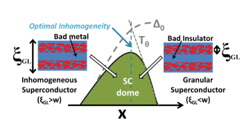

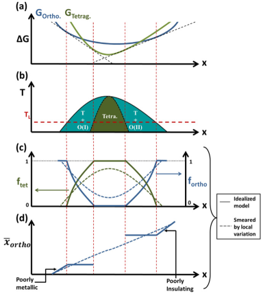
The family of bismuthate superconductors results from replacing K for Ba, or Pb for Bi, in BaBiO3, a charge density wave (CDW) insulator Uchida et al. (1987); Taraphder et al. (1996); Gabovich and Moiseev (1986); Baumert (1995). This family of superconductors has no magnetic degrees of freedom. Upon doping, the insulating CDW phase disappears, giving rise to a metallic phase where superconductivity appears at (maximum) temperatures below 30K and 11K for K-doping and Pb-doping, respectively Cava et al. (1988); Sleight et al. (1975). Structural phase separation on a nanoscopic scale has been observed in BaPb1-xBixO3 for superconducting compositions Giraldo-Gallo et al. (2012), but the implications in shaping the superconducting dome, in particular close to the disorder induced metal-insulator transition at 0.30 Luna et al. (2013) followed closely by the opening of a gap in the optical spectrum at 0.35, remain an open question. In this letter we report the observation of stripe-like structural phase separation in superconducting BaPb1-xBixO3 for compositions spanning optimal doping. Remarkably, the maximum occurs when the superconducting coherence length matches the size of the partially disordered stripes, implying a connection between the structural phase separation, the enhanced coulomb effects due to disorder (localization), the inhomogeneous superconducting properties, and the shape of the superconducting “dome” (see figure 1).
BaPb1-xBixO3 has a distorted perovskite (ABO3) crystal structure. For the highest Bi concentrations the material comprises two distinct Bi sites, with different Bi-O bond lengths. The origin of the associated charge density wave (CDW) has been widely debated Mattheiss and Hamann (1983); Varma (1988); Taraphder et al. (1996); Yin et al. (2013). For 0.8 the average structure comprises a single Bi/Pb site Marx et al. (1992), though EXAFS measurements reveal two distinct Bi-O bond lengths down to at least 0.25 Boyce et al. (1992), implying a persistence of the CDW at a local level. Significantly, for all compositions, the perovskite structure is also distorted by rotational instabilities of the oxygen octahedra, which can be described using Glazer’s notation Glazer (1972); Howard and Stokes (1998). For the insulating end-member compound BaBiO3 (), and down to , the unit cell space group is monoclinic I2/m (coming from a tilt, in Glazer’s notation); for the metallic end-member compound BaPbO3 () and up to , and again for , the unit cell space group is orthorhombic Ibmm (coming from a tilt, as shown in fig. 2(a)); however, for the region of , which is also the range of compositions for which the material is superconducting, the material is polymorphic, with a fraction of its volume with orthorhombic Ibmm symmetry and the rest with tetragonal I4/mcm symmetry (coming from a tilt) Climent-Pascual et al. (2011). The superconducting volume fraction peaks at the same Bi composition where the tetragonal-to-orthorhombic ratio is maximum, leading to the conclusion that the tetragonal polymorph is the one responsible for superconductivity in this material Climent-Pascual et al. (2011); Marx et al. (1992). This Bi composition is also the one for which the material has the maximum , i.e., the optimal doping composition.
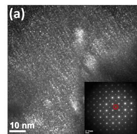
In the interest of investigating how the polymorphism is accommodated microscopically in a “single crystal” of BaPb1-xBixO3, and its possible consequences for the observed transport and, more interestingly, superconducting properties, high-resolution transmission electron microscopy (HRTEM) measurements were taken for samples with bismuth compositions below, at and above optimal doping. Samples of each concentration were crushed in liquid-nitrogen-cooled ethyl alcohol, and the liquid was allowed to warm to room temperature. The slurry was stirred and a small droplet was placed on a holey carbon grid and dried in air. The samples were analyzed using a FEI G2 F20TEM Tecnai STEM operated at 200 keV. Thin areas were analyzed with selected area diffraction, energy dispersive spectroscopy, and high-resolution imaging. Thin areas were aligned with either the 010 or the 001 zone axis based on indexing to the Ibmm structure (space group No. 74), showing clear lattice fringes in the HRTEM. All the HRTEM images taken for all the different compositions reveal a well-ordered structure, as can be observed in the 24.124.1nm2 image in fig. 2(b) for a sample with Bi composition of , and better appreciated in the 33nm2 expanded view in the inset to this figure. Fig. 2(c) shows its corresponding fast Fourier transform (FFT), revealing peaks from both tetragonal (hkl even) and orthorhombic (hkl even and odd, in the tetragonal notation) phases. In ref. Giraldo-Gallo et al. (2012) we showed that it is possible to recreate the spatial separation of the two polymorphs by systematically masking these diffraction peaks and performing an inverse Fourier transform (IFFT). In this way, we can obtain information about the length scales associated with the polymorphic variation across a sample.
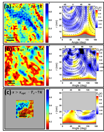
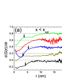
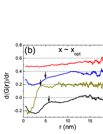
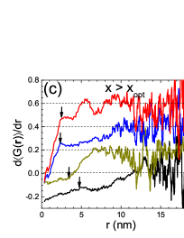
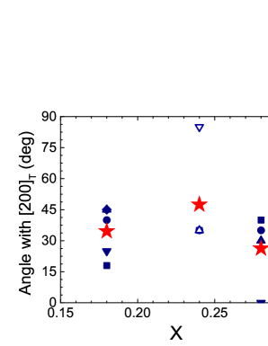
In order to quantify the length scales associated with the orthorhombic variation, the average spatial correlation function , and the angle-dependent spatial correlation function were computed for each 110/ filtered IFFT image (see supplemental material for definitions). Fig. 3 shows filtered-and-reconstructed HRTEM images for a representative sample of each Bi composition studied (left panels), after a resolution reduction from 0.47 per pixel, to 4.1 per pixel, therefore eliminating the atomic resolution information while keeping the longer-range variation in “orthorhombicity” (see supplemental material). Both, (shown in supplemental material) and (shown on the right panels of fig. 3) of all the images shown, reveal local minima and maxima, implying the presence of characteristic length scales for the phase separation. Furthermore, the angular dependent correlation function clearly reveals that there is a particular spatial pattern associated with the phase separation. Inspection of these quantities, in the right-hand panels of figure 3, reveals arcs of intensity with an approximately two-fold rotational symmetry. The arcs are imperfect, but repeat with a fixed periodicity, implying a self-organized pattern of phase separation over remarkably large length scales. Such a pattern of intensity in is consistent with a real space phase separation comprising partially disordered stripes (see supplemental material). For a system with stripes separated by a distance and running along an angle with respect to the horizontal, the distance between stripes as measured at an angle is given by (with ), which diverges at . As can be observed in Fig. 3 (and in similar data shown in the supplemental material), most of the samples studied exhibit this characteristic dependence, with periodic maxima (shown by solid lines in the figure) and minima (dashed lines) that approximately follow such an inverse cosine function. The orientation of the stripes with respect to the crystal axes is not identical for all images studied, but on average it is close to 2922∘ from the [100]T orientation. These stripes are clearly evident in the larger area real space images shown in the left hand panels of Fig. 3(a,b), running approximately top-left to bottom-right. In addition to the separation of stripes, inspection of the images in Fig. 3 reveals that there is a shorter (and more isotropic) length scale of structural variation, which describes the broken-up character of the stripes. This length scale can be seen more clearly in the average correlation function as a kink in the low-r tail, which can be better identified in the derivative of .
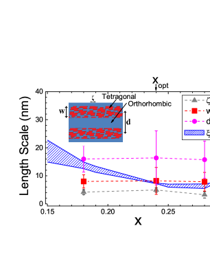
Although the stripe-like character of the structural phase separation is imperfect, nevertheless by identifying the morphology of the nanostructure we are able to define the characteristic length scales of phase separation in terms of three simple parameters (see inset to fig. 4): the stripe period, , (i.e. the distance between stripes of similar “orthorhombicity”, determined from the maxima of ); the stripe width, (estimated from the regions of minimum values in , i.e. stripes half-period, which can be used as a measure of the upper bound to the width of individual stripes); and the length scale associated with disorder within a stripe, , (identified in the derivative of the low-r tail of ). The analysis described above, was performed for a total of five samples, four samples and four samples (all of which are shown in the supplemental material), and the average value of , and for each Bi composition were calculated. The results are summarized in Fig. 4, together with the error obtained by calculating the standard deviation from the average value.
The phase separation of tetragonal and orthorhombic polymorphs is presumably driven by changes in the relative free energy of the two phases, both as a function of temperature and composition. The resulting morphology is reminiscent of spinodal decomposition, but the physical origin is somewhat different in this case, involving two competing phases (see supplemental material). Significantly, in such a scenario, the composition 0.24, at which the tetragonal volume fraction is maximal, marks the separatrix between formation of two different orthorhombic phases, both with the same structure, but one with a lower Bi concentration (for compositions ), and one with a higher Bi concentration (). Since the free energy of each polymorph can be affected by strain Lee et al. (1977), local variations in the local strain is anticipated to broaden or smear the otherwise sharp distinction in the variation of Bi composition. Considering the temperature dependence of the resistivity for compositions that have only an orthorhombic structure, it is clear that Bi substitution leads to a progressive evolution of the electronic properties of the orthorhombic phase from a “bad metal” for (i.e. , but with a very large absolute value of the resistivity) to a “bad insulator” for (i.e. , but nevertheless extrapolating to a finite conductivity at = 0) Giraldo-Gallo et al. (2012, 2013); Uchida et al. (1987). It is unclear whether this evolution of the electronic properties of the orthorhombic phase is driven by disorder due to the increasing Bi concentration, or a progressive increase in the CDW correlation length, or indeed a combination of both effects, but tunneling data clearly indicates that the zero temperature conductivity decreases to zero linearly in the entire range from 0 to 0.3, and that the associated zero bias tunneling anomaly also varies smoothly over this range Luna et al. (2013). Of particular significance for the following discussion, if the Bi concentration deviates from 0.24 in either direction, and the tetragonal volume fraction correspondingly diminishes, the phase separation results in small islands of superconducting tetragonal material with a characteristic length scale embedded in a matrix of orthorhombic BaPb1-xBixO3 that is either poorly conducting for or poorly insulating for . This distinction has important consequences for the evolution of the superconducting properties.
The significance of the structural modulation can be readily appreciated by comparing the associated length scales of the disordered stripes, , and (solid data points in fig. 4), with the Ginzburg-Landau coherence length, (blue curve in the same figure), for samples with , (optimally doped), and , with approximate values of 7K, 10.5K and 7K respectively. We estimate from , having used the standard Werthamer-Helfand-Hohenberg approximation to determine from . We employed both 50 and 90 criteria to extract from resistive transitions, leading to a narrow band of estimated values for . Inspection of Fig. 4 reveals that the three length scales associated with the phase separation are of the same order of magnitude as the superconducting coherence length, and largely independent of Bi concentration. The shortest length scale, , which characterizes the size of coherent regions within a given stripe, has a weak composition dependence, but does not grow to be larger than the superconducting coherence length for any composition, and is therefore expected to be less relevant than the larger length scales and associated with the period and width of the stripes. For low Bi concentrations, , the coherence length is larger than the width of individual stripes. However, at optimal doping, the width of individual stripes almost exactly matches the superconducting coherence length. Further increasing the Bi concentration appears to result in a saturation of which remains comparable to . This behavior is highly suggestive of an important role for the nanostructure in determining the shape of the superconducting dome, as we describe below.
In the context of an electronically-inhomogeneous system, where the coulomb potential seen by electrons varies spatially in a periodic way, with characteristic length , it has been shown theoretically that does not necessarily track the pairing scale , i.e. the superconducting gap magnitude Kivelson and Fradkin (2007). Rather, the evolution of is bounded above by two parameters: the pairing scale and the phase ordering temperature . In the limit where (where is the superconducting coherence length), , and will be determined by . However, in the limit , the phase ordering temperature is small compared to the pairing amplitude , and is entirely determined by , meaning that is suppressed with respect to . In this regime the material behaves as a granular superconductor, characterized by superconducting “islands” that are only weakly coupled. For a system where the length scale of phase separation evolves with respect to the superconducting coherence length (or vice-versa), the maximum value is obtained in the crossover regime of the curves of and , which happens at . This regime has been dubbed “optimal inhomogeneity”Kivelson and Fradkin (2007); Arrigoni and Kivelson (2003). In the case of BaPb1-xBixO3, the phase separation is not necessarily refering to electronic phase separation due to variations in coulomb interaction, but rather the local variation in pairing interaction of the two coexisting polymorphs, although a similar set of arguments clearly applies.
The phenomenology of BaPb1-xBixO3 appears to be consistent with such a scenario, in which tetragonal and orthorhombic polymorphs correspond to regions of the bulk material with large and small pairing interactions respectively. The evolution with doping of the relative length scales characterized by and the phase separation is very suggestive of optimal doping being a turning point from a macroscopic inhomogeneous superconductor (with bigger than other characteristic length scales associated with disorder) for to a phase-fluctuation-dominated granular superconductor for (illustrated schematically in figure 1). Indeed, several signatures of granular superconductivity are observed in this regime, such as negative magnetoresistance for fields above , and scaling reminiscent of a superconductor-insulator quantum phase transition Giraldo-Gallo et al. (2012). Additionally, scanning tunneling spectroscopy (STS) measurements for compositions beyond optimal doping show a large variation in gap values as a function of position, with maximum values exceeding those found in the higher optimally doped material Parra et al. (2014), suggesting that samples with have a larger local pairing amplitude than expected for their macroscopic , and even for an 11 K superconductor. This observation is consistent with a macroscopic being bounded by the phase ordering line, , i.e., with a granular superconductor picture (see figure 1). Significantly, these observations imply that for the superconducting phase of this material (the tetragonal polymorph) is in fact a higher-temperature superconductor, possibly even comparable to the other bismuthate superconductor Ba1-xKxBiO3 Luna et al. (2013).
In the above analysis, the only significance of the stripe-like character of the nanostructure of BaPb1-xBixO3 has been that it has enabled us to establish the characteristic length-scales with a little more precision than if we had assumed a more isotropic morphology. However, the stripe-like morphology possibly has a much deeper significance. In the context of BaPb1-xBixO3, this might provide a natural means to understand the unusual scaling behavior observed at the superconductor-insulator transition close to optimal doping in this material Giraldo-Gallo et al. (2012, 2013), motivating theoretical investigation of percolation effects near the quantum phase transition for a material with a “stripy” morphology. More broadly, several families of underdoped cuprates have been shown to exhibit stripe and/or unidirectional CDW formation Tacon et al. (2014); Tranquada et al. (1995); Howald et al. (2003). In the case of the cuprates, the stripe/CDW order is driven by spontaneous electronic order, whereas for the bismuthates the stripe-like nanostructure is quenched from higher temperature Cava (2012). Significantly, in both cases, the stripe-like phase separation and superconductivity are found to have comparable length scales. In this broader context, BaPb1-xBixO3 provides a model system to explore the effects of stripe-like phase separation on superconductivity, and in particular on the associated phenomenology of optimal inhomogeneity.
The authors thank S. A. Kivelson for helpful discussions. This work is supported by AFOSR Grant No. FA9550-09-1-0583. The electron microscopy was performed at Ames Laboratory (Y.Z. and M.J.K.) and supported by the U.S. Department of Energy (DOE), Office of Basic Energy Science (BES), Division of Materials Sciences and Engineering, under Contract No. DE-AC02-07CH11358. C.P. and H.C.M. were supported by US Department of Energy (DOE), Office of Science, Basic Energy Sciences (BES), Materials Sciences and Engineering Division, under contract DE-AC02-76SF00515.
Appendices
Appendix A Glazer’s notation
The ideal cubic perovskite ABO3, described by the space group , can be represented as a network of corner-sharing BO6 octahedra. ‘A’ atoms sit in the geometric center of the gap between oxygen octahedra. This structure is a “simple” and highly symmetric one; however, most materials with perovskite structures are not in their ideal cubic form, but their structure can nevertheless be represented as coming from distortions from this ideal configuration. The types of distortions found in perovskites can be narrowed down to three types: B-cation displacements within an octahedra; distortions of the BO6 octahedral unit; and, the most common one and subject of this section, and of Glazer’s study Glazer (1972), the rigid tilting of the corner-sharing BO6 linked-octahedra units. This last type of distortion was described by Glazer in terms of tilt components along the three different pseudocubic (PC) axes, referred to the original undistorted cubic perovskite. Such pseudocubic axes coincide with the tetrad axes of the octahedra. Given the octahedra corner connections, a tilt about a pseudocubic axis determines the tilts in the directions perpendicular to this axis. However, the tilt of the successive octahedra along the same axis can be either in the same direction or in the opposite direction. With this in mind, the different possibilities of tilt-distortions can be labeled by the notation , where , , refer to tilts around the , and axes, respectively. If letters are repeated, the tilts are equal for their respective axis. The superscript can be either , for no-tilt along an axis; , for tilt of successive octahedra in the same sense; or , for tilt of successive octahedra in the opposite sense Howard and Stokes (1998). For example, the I4/mcm space group is represented by the notation , which means zero tilt about the and axes, and finite tilt about the axis, with opposite rotation of the successive octahedra along this axis. The Ibmm space group is represented by the notation , which means equal tilts about the and axes (equivalent to a tilt about the direction), with opposite rotation of the successive octahedra along these axes, and zero tilt about the axis.
Appendix B Electron diffraction patterns
Simulated electron diffraction patterns for tetragonal I4/mcm and orthorhombic Ibmm polymorphs of BaPb1-xBixO3 along the and zone axis were obtained through the University of Illinois web-based electron microscopy application software (WEB-EMAPS) Zuo and Mabon (1992), using the atomic parameters shown in tables 1 and 2. Along both of these zone axis, the set of reflections with even, are common to both, orthorhombic and tetragonal phases. However, for both zone axes, the set of reflections with odd, appears only in the orthorhombic phase and not in the tetragonal. In ref. 14 we showed that it is possible to recreate the spatial separation of the two polymorphs by systematically masking these diffraction peaks and performing an inverse Fourier transform (IFFT). The result of applying a mask such that only the even peaks, common to both the tetragonal and orthorhombic phases, show an ordered array of planes of atoms (see figure 6 in ref. 14). In contrast, the result of applying a mask to the peaks, attributed only to the Ibmm orthorhombic phase, reveals a spatial variation due to the densely intergrown nanostructure, as shown in Fig. 3 of the main manuscript, and Figs. A3, A4 and A5 of this supplemental material.
| Atom | Wyck. | Site | x/a | y/b | z/c |
|---|---|---|---|---|---|
| Ba | 4b | -42m | 0 | 0.5 | 0.25 |
| Pb/Bi | 4c | 4/m | 0 | 0 | 0 |
| O1 | 8h | m.2m | 0.2179(14) | 0.7179(14) | 0 |
| O2 | 4a | 422 | 0 | 0 | 0.25 |
| Atom | Wyck. | Site | x/a | y/b | z/c |
|---|---|---|---|---|---|
| Ba | 4e | mm2 | 0.496 | 0 | 0.25 |
| Pb/Bi | 4a | 2/m | 0 | 0 | 0 |
| O1 | 4e | mm2 | 0.0496 | 0 | 0.25 |
| O2 | 8g | .2. | 0.25 | 0.25 | 0.9741 |
Appendix C Definition of the correlation function
The spatial autocorrelation function of an image is defined as the statistical correlation of two points separated by a vector , where and are the positions of those two points in the image Fratini et al. (2010).
| (1) |
where
| (2a) | ||||
| (2b) | ||||
| (2c) | ||||
| (2d) | ||||
| (2e) | ||||
The average spatial autocorrelation function is the result of averaging the correlation function of all vectors with the same magnitude . The angle-dependent autocorrelation function is the result of averaging the correlation function of all vectors with orientation with respect to the horizontal axis, and magnitude .
Appendix D Correlation function for reduced-resolution images
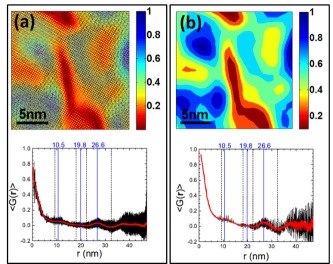
Fig. A1(a) shows a 1919nm2 portion of the 110 filtered IFFT of the HRTEM image in fig. 2(b) of the main manuscript. This image keeps the information of both the atomic periodicity as well as a larger-scale contrast variation, reflecting variations in the local “orthorhombicity” across the sample. The image in figure A1(b) is the result of a resolution reduction by adjacent averaging, of the image in fig. A1(a), from 0.47 per pixel, to 7.5 per pixel, therefore eliminating the atomic resolution information while keeping the longer-range variation in “orthorhombicity”. The bottom parts of fig. A1(a) and A1(b) show the computed average spatial correlation functions of their respective images on top. The vertical lines in label local minima and maxima positions , being equivalent for both, the original resolution image in fig. A1(a), and the reduced resolution image in fig. A1(b). For the purpose of our analysis, we consider only the reduced resolution images, given that these conserve the information of the longer-scale structural variation while reducing the computational requirements.
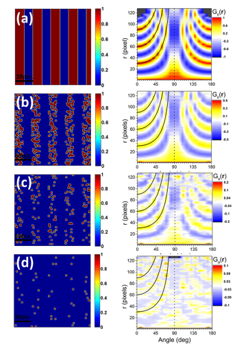
Appendix E Correlation function for a stripe model
The angular dependent correlation function was computed for an image of size 128128 pixels, showing perfect stripes formation, with stripes of width 15 pixels and periodicity 30 pixels, running along an angle 90∘ with respect to the horizontal axis (fig. A2(a)). The color scale of the right hand side plot of fig. A2(a) represents the value of , as a function of the angle with the horizontal axis and the magnitude of . Maxima of for this image appear along arcs following the functional form (shown by the black solid lines), where . Figures A2(b)-(d) show images of the same size and with stripes of the same width and periodicity as in (a), but where a progressively broken-up character has been introduced for each image. For these images, the maxima of follow in average the same functional form as the original zero-disorder stripe model, but the local maximum value of progressively decreases in value, from 1 for the perfect-stripes image in fig. A2(a), to about 0.1 for the most broken-up image in fig. A2(d). At the same time, the arcs where the maximum values of appear get progressively more broken-up, although its average functional form is preserved, and its periodicity can be well identified. The angle dependent correlation functions observed in the filtered-and-reconstructed images analyzed throughout this article show very similar features to the ones observed in this model of broken-up stripes.
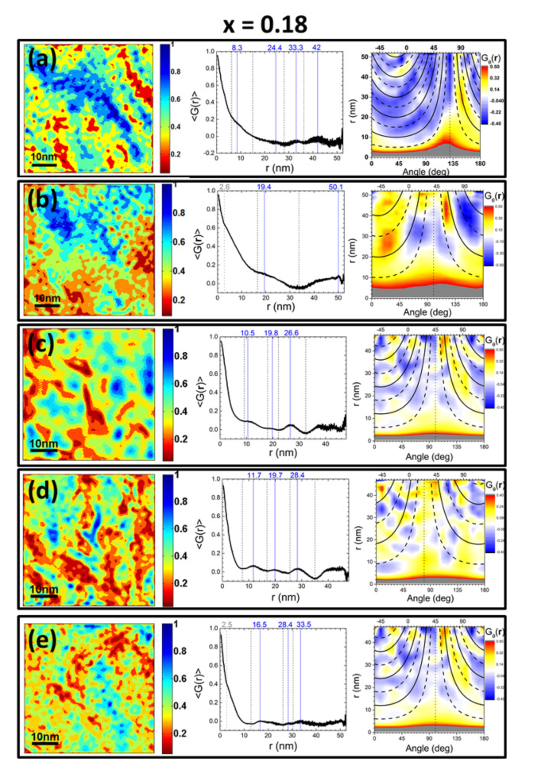
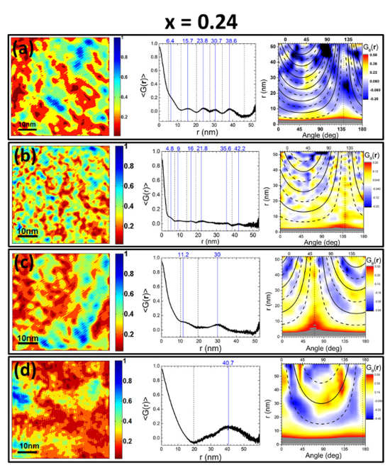
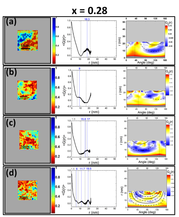
Appendix F Correlation function for all the images studied
Figures A3, A4 and A5 of this supplemental material show filtered-and-reconstructed images (left-hand panels) for a total of five samples (fig. A3), four samples (fig. A4) and four samples (fig. A5), as well as their respective average spatial correlation function (central panels) and angle-dependent spatial correlation function (right-hand panels). The first image of each figure had been already shown in figure 3 of the main manuscript; however it is shown again for completeness and with the spirit of presenting the average correlation function that was not presented before. The characteristic length scales of phase separation shown in figure 4 of the main manuscript are: (1) stripes periodicity, , (2) stripes width, , and (3) the correlation length within a single stripe, . These length scales were determined for all of the figures, and the average value for each quantity determined and plotted as a function of Bi concentration in Fig. 4 of the main manuscript.
Appendix G Derivative of the average correlation functions
The length-scale representing the disorder within a stripe, denoted as , is picked-up more clearly in the average correlation function , as a kink or change of slope in the low-r tail region. This kink is more precisely seen in the derivative of this quantity, as shown in figure A6(a,b,c) for the different Bi compositions and samples of each compositions studied. Black arrows in these plots show the points determining the value of for each sample. The average value of is plotted in figure 4 of the main manuscript, together with the other length scales of phase separation.
Appendix H Orientation of stripes
Fig. A7 shows the orientation of stripes with respect to the axis, for all the different samples studied, as a function of Bi concentration. The uncertainty of this measure is large given the imperfect character of the stripe patterns, however, it can be observed that the average value is close to 30∘ from the axis (2922∘).
Appendix I Phase separation model
The phase separation of tetragonal and orthorhombic polymorphs in BaPb1-xBixO3 is presumably driven by changes in the relative Gibbs free energy of the two phases, both as a function of temperature and composition Fisher et al. (2012). Such a scenario is illustrated schematically in fig. A8. The resulting morphology is reminiscent of spinodal decomposition, but the physical origin is somewhat different in this case, involving two competing phases. The point where the maximum tetragonal fraction is found, which for the case of BaPb1-xBixO3 is coincident with optimal doping, 0.24, demarks a separatrix between a low-Bi orthorhombic phase, O(I), for compositions , and a Bi-rich orthorhombic phase, O(II), for compositions . It has been previously shown for various metallic precipitates embedded in metallic matrices (Cu-in-Al, Ag-in-Cu, Ag-in-Al, among others) that inhomogeneous strain can cause local variations in the free-energy, modifying phase equilibria Lee et al. (1977). Therefore, it is reasonable to anticipate that the sharp distinctions in composition between the O(I) and O(II) phases will be blurred in practice (see panels (c) and (d) of figure A8). The resulting continuous variation in composition, and presumably lattice parameter, is consistent with results of recent x-ray and neutron diffraction measurements Climent-Pascual et al. (2011). Consequently, the resistivity of the orthorhombic matrix in which the tetragonal polymorph resides, evolves continuously from that of a poor metal to a poor insulator.
Appendix J Dark-field TEM images
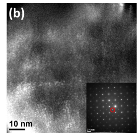
In addition to the HRTEM images used in the analysis presented throughout this work, dark-field (DF) TEM images were also taken. These images also reveal the presence of broken-up stripes, with length scales consistent with the ones obtained through the filtered-and-reconstructed HRTEM images analysis described in the main text. Fig. A9(a,b) shows DF images for samples with Bi concentration of 0.18 and 0.28, respectively, along the zone axis. These DF images were obtained using the reflection shown in the red circle in the insets to fig. A9(a,b). For both figures the size and distribution of the bright regions, imaged using reflection limited to the Ibmm phase, mimics the small patchwork of coherent domains seen in the Fourier-filtered reconstruction. A stripy pattern, containing patches of 5-10nm, which for image in fig. A9(a) is more scattered throughout, is better seen in the image in fig. A9(b), and the length-scales observed are consistent with the ones found with the Fourier-filtered reconstruction. Note that only one of the four reflections are used in the DF image, while Fourier-filtered reconstruction uses all of the reflections in the reconstruction. This is most likely the cause of the directionality seen in the image in figure A9(a).
Appendix K Intensity probability distributions
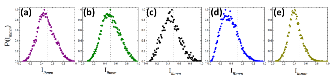
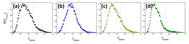
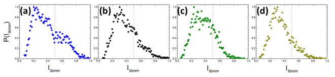
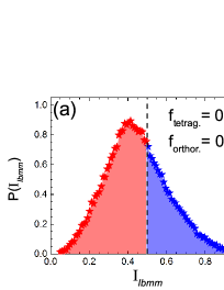
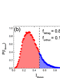
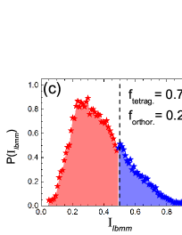
We also computed the probability distribution of intensities of the filtered-and-reconstructed HRTEM images shown in Fig. 3 of the main text, and in Figs. A3, A4 and A5 of this document. For each image, the intensity in each pixel, which might be labelled the intensity of “orthorhombicity”, was normalized by the maximum intensity in the image, so that for all of the images this quantity goes from 0 to 1. Then, we computed the histogram of intensity, dividing the range of intensity into 100 sections. The vertical scale (counts) of each histogram is then normalized, so that for all the images this scale goes from 0 to 1. These curves are proportional to the probability distribution of intensity. The results for each image studied in this work are shown in fig. A10 for samples with Bi concentration 0.18, in fig. A11 for samples with 0.24, and in fig. A12 for samples with 0.28. For each composition, all the normalized histograms were averaged, and the result of this averaging is shown in fig. A13. From these averaged histograms we estimated the orthorhombic filling fraction, , as the normalized-integrated area above half the total intensity (as shown in the blue-shadowed areas in fig. A13).
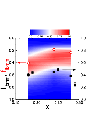
The evolution of the orthorhombic volume fraction as a function of Bi concentration can be better visualized in fig. A14. The left axis of this figure shows an inverted scale (from 1 to 0) of the orthorhombic intensity. The colors in the contour plot represent values of the probability of “orthorhombicity”, i.e., the y scale in the averaged histograms shown in fig. A13, as a function of orthorhombic intensity and Bi concentration. From this figure we can observe that the maximum of the probability distribution of “orthorhombicity” (red colors) is shifted toward lower values of orthorhombicity for optimal doping, compared to samples with lower and higher Bi concentrations. As a consequence, if we represent the orthorhombic volume fraction as the normalized-integrated area above half the total intensity, it is minimum at optimal doping, which means that the tetragonal fraction, is maximum at this composition, with a value of 0.820.08. The evolution of the inverse of the orthorhombic fraction, ie., the tetragonal fraction, approximately tracks the evolution of the superconducting volume fraction, shown in the right scale and as black squares. These observations are consistent with results from x-ray and neutron diffraction experiments by E. Climent-Pascual et al.Climent-Pascual et al. (2011) in polycrystalline samples, and suggest a direct connection between the tetragonal distortion and superconductivity.
References
- Tranquada et al. (1995) J. M. Tranquada, B. J. Sternlieb, J. D. Axe, Y. Nakamura, and S. Uchida, Nature 375, 561 (1995).
- Howald et al. (2003) C. Howald, H. Eisaki, N. Kaneko, M. Greven, and A. Kapitulnik, Phys. Rev. B 67, 014533 (2003).
- Tacon et al. (2014) M. L. Tacon, A. Bosak, S. M. Souliou, G. Dellea, T. Loew, R. Heid, K.-P. Bohnen, G. Ghiringhelli, M. Krisch, and B. Keimer, Nature Phys. 10, 52 (2014).
- Kivelson and Fradkin (2007) S. A. Kivelson and E. Fradkin, Treatise of High Temperature Sureconductivity: Chapter 15 (Springer, 2007).
- Kivelson et al. (2003) S. A. Kivelson, I. P. Bindloss, E. Fradkin, V. Oganesyan, J. M. Tranquada, A. Kapitulnik, and C. Howald, Rev. Mod. Phys. 75, 1201 (2003).
- Berg et al. (2008) E. Berg, D. Orgad, and S. A. Kivelson, Phys. Rev. B 78, 094509 (2008).
- Climent-Pascual et al. (2011) E. Climent-Pascual, N. Ni, S. Jia, Q. Huang, and R. J. Cava, Phys. Rev. B 83, 174512 (2011).
- Uchida et al. (1987) S. Uchida, K. Kitazawa, and S. Tanaka, Phase Transitions 8, 95 (1987).
- Taraphder et al. (1996) A. Taraphder et al., International J. of Mod. Phys. B 10, 863 (1996).
- Gabovich and Moiseev (1986) A. M. Gabovich and D. P. Moiseev, Sov. Phys. Usp. 29, 1135 (1986).
- Baumert (1995) B. A. Baumert, J. Supercond. 8, 175 (1995).
- Cava et al. (1988) R. J. Cava et al., Nature 332, 814 (1988).
- Sleight et al. (1975) A. W. Sleight, J. L. Gillson, and P. E. Bierstedt, Solid State Commun. 17, 27 (1975).
- Giraldo-Gallo et al. (2012) P. Giraldo-Gallo, H.-O. Lee, Y. Zhang, M. J. Kramer, M. R. Beasley, T. H. Geballe, and I. R. Fisher, Phys. Rev. B 85, 174503 (2012).
- Luna et al. (2013) K. Luna, P. Giraldo-Gallo, T. H. Geballe, I. R. Fisher, and M. R. Beasley, Arxiv: 1311.4212v1 (2013).
- Mattheiss and Hamann (1983) L. F. Mattheiss and D. R. Hamann, Phys. Rev. B 28, 4227 (1983).
- Varma (1988) C. M. Varma, Phys. Rev. Lett. 61, 2713 (1988).
- Yin et al. (2013) Z. P. Yin, A. Kutepov, and G. Kotliar, Phys. Rev. X 3, 021011 (2013).
- Marx et al. (1992) D. T. Marx, P. G. Radaelli, J. D. Jorgensen, R. L. Hitterman, D. G. Hinks, S. Pei, and B. Dabrowski, Phys. Rev. B 46, 114 (1992).
- Boyce et al. (1992) J. B. Boyce, F. G. Bridges, T. Claeson, T. H. Geballe, G. G. Li, and A. W. Sleight, Phys. Rev. B 46, 114 (1992).
- Glazer (1972) A. M. Glazer, Acta Cryst. B28, 3384 (1972).
- Howard and Stokes (1998) C. J. Howard and H. T. Stokes, Acta Cryst. B54, 782 (1998).
- Lee et al. (1977) J. K. Lee, D. M. Barnett, and H. I. Aaronson, Metallurgical Transactions A 8, 963 (1977).
- Giraldo-Gallo et al. (2013) P. Giraldo-Gallo, H.-O. Lee, M. R. Beasley, T. H. Geballe, and I. R. Fisher, J. Supercond. and Nov. Magn. 26, 2675 (2013).
- Arrigoni and Kivelson (2003) E. Arrigoni and S. A. Kivelson, Phys. Rev. B 68, 180503 (2003).
- Parra et al. (2014) C. Parra, F. C. Niestemski, A. W. Contryman, P. Giraldo-Gallo, T. H. Geballe, I. R. Fisher, and H. C. Manoharan, To be published (2014).
- Cava (2012) R. J. Cava, private communication (2012).
- Zuo and Mabon (1992) J. Zuo and J. C. Mabon, “Web-based electron microscopy application software: Web-emaps.” University of Illinois. http://emaps.mrl.uiuc.edu. (1992).
- Fratini et al. (2010) M. Fratini, N. Poccia, A. Ricci, G. Campi, M. Burghammer, G. Aeppli, and A. Bianconi, Nature 466, 841 (2010).
- Fisher et al. (2012) I. R. Fisher, M. C. Shapiro, and J. G. Analytis, Philosophical Magazine 92, 19 (2012).