Thermodynamic bounds and general properties of optimal efficiency and power in linear responses

Abstract

We study the optimal exergy efficiency and power for thermodynamic systems with Onsager-type “current-force” relationship describing the linear-response to external influences. We derive, in analytic forms, the maximum efficiency and optimal efficiency for maximum power for a thermodynamic machine described by a $N\times N$ symmetric Onsager matrix with arbitrary $N$. The figure of merit is expressed in terms of the largest eigenvalue of the “coupling matrix” which is solely determined by the Onsager matrix. Some simple but general relationships between the power and efficiency at the conditions for (i) maximum efficiency and (ii) optimal efficiency for maximum power are obtained. We show how the second law of thermodynamics bounds the optimal efficiency and the Onsager matrix, and relate those bounds together. The maximum power theorem (Jacobi’s Law) is generalized to all thermodynamic machines with symmetric Onsager matrix in the linear-response regime. We also discuss systems with asymmetric Onsager matrix (such as systems under magnetic field) for a particular situation and we show that the reversible limit of efficiency can be reached at finite output power. Cooperative effects are found to improve the figure of merit significantly in systems with multiply cross-correlated responses. Application to example systems demonstrates that the theory is helpful in guiding the search for high performance materials and structures in energy researches.

I Introduction

Under challenges imposed by increasing demand yet limited availability of energy resources, improving energy efficiency becomes increasingly important in technology developments. Historically, Carnot deduced that for a heat engine operating between two reservoirs with temperatures $T_{h}$ and $T_{c}$ ($T_{h}>T_{c}$), the energy conversion efficiency, $\eta=W/Q$ ($W$ is the output work, $Q$ is the heat from the hot reservoir), has a maximum value, namely the Carnot efficiency, $\eta_{C}=(T_{h}-T_{c})/T_{h}$callen . The Carnot efficiency is only for ideal machines operating in the reversible limit. Energy efficiency of realistic machines is reduced by unavoidable irreversible entropy production. A way to count the reduction of energy efficiency from the value at reversible limit is to use the exergy efficiency (or “second-law efficiency”)odum ; 2ndlaw1 ; 2ndlaw2 ; 2ndlawbook ; caplan1 ; caplan2

$$\phi\equiv\frac{\dot{\cal A}_{out}}{\dot{\cal A}_{in}}$$ (1)

where $\dot{\cal A}_{out}$ and $\dot{\cal A}_{in}$ are the output and input exergy (i.e., the Gibbs free energy) per unit time. Exergy is defined as ${\cal A}={\cal U}-TS$ where ${\cal U}$ is the enthalpy (i.e., the total energy), $T$ is the temperature, and $S$ is the entropy. Although the total energy is conserved, the output exergy is reduced by entropy production, $\dot{S}_{tot}$, as $\dot{\cal A}_{out}=\dot{\cal A}_{in}-T\dot{S}_{tot}$, hence $\phi\leq 1$. Both $\phi\leq 1$ and $\eta\leq\eta_{C}$ are dictated by the second law of thermodynamics. In fact for thermoelectric engine and refrigerator the two are related byodum ; 2ndlawbook ; caplan1 ; ca-ex ; Seifert-review

$$\phi=\frac{\eta}{\eta_{C}}.$$ (2)

For this reason, exergy efficiency is also called as “rational efficiency”2ndlawbook . Using Onsager’s theory of irreversible thermodynamics and the exergy efficiency, the study of efficiency of heat engines, chemical engines, and other energy devices can be presented in an uniform mannerca-ex ; Seifert-review ; odum ; 2ndlaw1 ; 2ndlaw2 ; 2ndlawbook ; caplan1 ; caplan2 . Specifically, the efficiency of chemical engines, the output work divided by the chemical work, is precisely Eq. (1), as the output work is equal to the output exergy and the input chemical work is equal to the input (consumed) exergyca-ex ; Seifert-review ; 2ndlaw1 . The exergy efficiency becomes particularly convenient for machines with multiple forms of input (or output) energycaplan2 . For example in a spin-thermoelectricbauer refrigerator, both electrical energy and magnetic energy are consumed to drive the cooling (see Sec. VI.2).

A central issue in energy application is to find out the optimal efficiency and maximum power of a machine and the conditions that realize themdevos ; ca ; nicolis . For example, Ioffe derived the optimal exergy efficiency for isotropic thermoelectric materials in the linear-response regime asioffe

$$\eta_{max}=\eta_{C}\frac{\sqrt{\xi+1}-1}{\sqrt{\xi+1}+1},\quad\quad\xi=\frac{\sigma S^{2}T}{\kappa}.$$ (3)

The figure of merit, $\xi$, is solely determined by the transport coefficients of the material: the electrical conductivity $\sigma$, the Seebeck coefficient $S$, and the thermal conductivity $\kappa$. This property is an important guiding principle in the search of high performance thermoelectric materialshonig ; ms ; review .

However, Eq. (3) was derived for isotropic systems, where, by choosing a proper set of coordinate axes, the problem can be reduced to correlated transport for two scalar currents: one heat current and one electric current. Quite often in anisotropic materials, the complete description of thermoelectric transport must involve six scalar currents as both the electric and heat currents consist of three scalar components (e.g., the electrical current $\vec{j}=(j_{x},j_{y},j_{z})$ with $j_{x}$, $j_{y}$, and $j_{z}$ being the components in the $x$, $y$, and $z$ directions)honig ; aniso . For piezoelectric energy conversion in an anisotropic material, the full description of responses involves nine scalar “currents”: three of them are electric displacements and the other six are strainspe . The description of these cross-correlated responses can be simplified only for certain high symmetry structures. Recent development of technologies for high-quality thin film growth which allows precise control of composition, atomic arrangements and interfaces provides the toolbox for functional nano-structured composite materials which could have pronounced application values that does not share by their compounds. Often these composite structures have lower symmetry and the full description of cross-correlated responses cannot be simplified. Besides, breaking time-reversal symmetry brings further complication to cross-correlated responsestrb1 ; trb2 ; trb3 . Quite often Ioffe’s derivation of optimal energy efficiency cannot be directly applied to those practical systems. In those situations the (global) maximum efficiency is rather difficult to find, although one can always easily find certain optimal efficiencies under restrictionshonig ; aniso ; multi ; pe ; caplan2 .

Finding the optimal exergy efficiency and power for complex thermodynamic systems has stimulated a number of studiesaniso ; bio ; caplan2 . It becomes increasingly important as researches reveal more cross-correlated responses and realize their applicationsbauer ; zlwang1 ; zlwang2 . Fast developing nanotechnologies and material technologies offer a large number of materials and structures of which complex cross-correlated responses are enhanced and made available for practical applications. Examples are, spin-thermoelectric effectbauer , piezopotential gatingzlwang1 and piezo-phototronicszlwang2 , to name but just a few. Besides, biological systems are often characterized by cross-correlated responses to density, temperature, and electrochemical potential gradientsbio ; caplan2 . A typical example is transport across a biological membrane: even for a single ionic solution, transmission through the membrane must be described by three flows, the volume flow, the solute flow, and the electrical flow, which are often cross-correlatedbio . Cross-correlated responses enable energy conversion from one form to another, during which the functions of a machine is realized (a “machine” is a system which consumes input energy to achieve a practical goal by doing work to the external). Caplan derived the analytic expression of the optimal exergy efficiency for machines with only one flow for energy input but multiple flows for output or vice versacaplan2 . However, general results on the optimal efficiency and power are still absent, particularly in analytic forms.

In this work we derive analytic results for optimal efficiency and power under general considerations that can be applied to a broad range of thermodynamic systems. The requirements are only that there exists an Onsager-type “current-force” relation that describes the responses to external influences (“forces”)onsager and that the system is operating at steady states in linear responses. These requirements are often satisfied for physical systems with forces not too stronggroot ; nicolis . The derived results can be connected with realistic systems of which the output power is consumed by a device or by large a power grid. We obtain some simple but general relationships that connect the optimal power and efficiency for different optimization schemes. These results are first obtained for systems with symmetric Onsager response matrix and then extended to systems with asymmetric Onsager matrix (e.g., systems under magnetic field). We point out that cooperative effects can be used to improve efficiency (figure of merit) for systems with multiple cross-correlated responses. Such improvement, achieved via combining different input (or output) forces rather than engineering materials, can be significant in systems with multiple cross-correlated responses. Examples are given to demonstrate how the theory is used to guide the search for high performance energy applications.

This paper is organized as follows: in Sec. II we establish the basic formalism by using Onsager’s theory of irreversible thermodynamic processes in the linear-response regime. We derive the optimal efficiency and output power for symmetric Onsager matrix in Sec. III. In Sec. IV the derivation is re-interpreted with realistic considerations where parasitic dissipation and the response of the device accepting the output energy are considered. We extend the study to systems with asymmetric Onsager matrix in Sec. V. Examples that illustrate the usefulness of the findings are presented in Sec. VI, and we conclude in Sec. VII.

II Basic formalism

Under external influences (“forces”) a thermodynamic system develops motions that deviate from their equilibrium values. These motions (“currents”) can be described quantitatively by the rates of changes in thermodynamic state variablesgroot ; landau . The relation between the forces $\vec{{\cal F}}$ and currents $\vec{{\cal J}}$ is generally written asgroot ; landau

$$\vec{{\cal J}}=\hat{{\cal M}}\vec{{\cal F}}\quad{\rm or}\quad{\cal J}_{n}=\sum_{k}{\cal M}_{nk}{\cal F}_{k},$$ (4)

where the index $n$ ($k$) numerates all currents (forces), and $\hat{{\cal M}}$ is the Onsager matrix. When the forces are not too strong the dependence of $\hat{{\cal M}}$ on the forces can be ignored. Cross-correlated responses (e.g., thermoelectric effect) allow energy conversion from the input forms to the output forms and realize functions of a machine. According to the theory of irreversible thermodynamicsonsager ; groot , there are an equal number of forces and currents. Each force ${\cal F}_{n}$ has a conjugated current ${\cal J}_{n}$ such that the reduction of total exergy (Gibbs free energy) is given by

$$-\dot{\cal A}_{tot}=T\dot{S}_{tot}=\sum_{n}{\cal J}_{n}{\cal F}_{n}.$$ (5)

The reduction of exergy $-\dot{\cal A}_{n}={\cal J}_{n}{\cal F}_{n}$ associated with the current ${\cal J}_{n}$ for exergy input is positive, while for exergy output it is negative. Hence the input and output exergy arecaplan2

$$\dot{\cal A}_{in}\equiv\sum_{n\in I}{\cal J}_{n}{\cal F}_{n},\quad\dot{\cal A}_{out}\equiv-\sum_{k\in O}{\cal J}_{k}{\cal F}_{k},$$ (6)

respectively. The sets $I$ and $O$ in the above refer to exergy input and output, respectively. The output exergy is also the output work, i.e., $\dot{W}=\dot{\cal A}_{out}$ (Throughout this paper “work” is associated with linear-response processes for given thermodynamic forces, i.e., work and efficiency are functions of thermodynamic forces). For $\dot{\cal A}_{in}>0$ the exergy efficiency is

$$\phi=\frac{-\sum_{k\in O}{\cal J}_{k}{\cal F}_{k}}{\sum_{n\in I}{\cal J}_{n}{\cal F}_{n}}=\frac{\dot{\cal A}_{in}-T\dot{S}_{tot}}{\dot{\cal A}_{in}}\leq 100\%.$$ (7)

Only in the reversible limit, $\dot{S}_{tot}=0$, the exergy efficiency $\phi$ reaches its upper bound. The second law of thermodynamics requires $\dot{S}_{tot}\geq 0$ for all possible values of forces. This is satisfied only when all eigenvalues of the Onsager matrix $\hat{{\cal M}}$ are positive [see Appendix A] (note that, as the reversible limit, $\dot{S}_{tot}=0$, does not exist for realistic systems, we consider only situations with positive entropy production. Zero entropy production is the limit when the entropy production is extremely small. In this way, all eigenvalues of the Onsager matrix must be greater than zero.) This property is briefly stated as that Onsager matrix is positive.

III Optimizing efficiency and power for systems with symmetric Onsager matrix

The maximum exergy efficiency is obtained by solving the differential equation

$$\partial_{{\cal F}_{k}}\phi=0,\quad\forall k.$$ (8)

Previous attempts of solving the above equationsaniso ; bio ; caplan2 have ended up with very complicated calculations and discussions. This is because for a $N\times N$ Onsager matrix, there are $N(N+1)/2$ independent response coefficients (if the Onsager matrix is symmetric). Besides, there are $N-1$ coupled differential equations to solve (from Eqs. (4) and (7), scaling all forces by a constant does not change $\phi$; this property reduces the number of differential equations to be solved by one). Solving these equations analytically becomes a formidable task when $N\geq 3$ (see, e.g., the rather complicated discusssions in Ref. caplan2 ). In this work we manage to solve the problem analytically in a particularly simple way.

We notice that the force-current relation can be rewritten as

$$\left(\begin{array}[]{c}\vec{{\cal J}}_{O}\\ \vec{{\cal J}}_{I}\end{array}\right)=\left(\begin{array}[]{cccc}\hat{{\cal M}}_{OO}&\hat{{\cal M}}_{OI}\\ \hat{{\cal M}}_{IO}&\hat{{\cal M}}_{II}\end{array}\right)\left(\begin{array}[]{c}\vec{{\cal F}}_{O}\\ \vec{{\cal F}}_{I}\end{array}\right),$$ (9)

where the symbols $O$ and $I$ are used to abbreviate the indices of forces and currents for exergy output and input, respectively. E.g., $\vec{{\cal J}}_{O}$ is the vector of the output current and $\hat{{\cal M}}_{OO}$ is the matrix relating the output force vector $\vec{{\cal F}}_{O}$ to the output current vector $\vec{{\cal J}}_{O}$. Hence,

$$\dot{\cal A}_{out}=-\vec{{\cal F}}_{O}^{T}\hat{{\cal M}}_{OI}\vec{{\cal F}}_{I}-\vec{{\cal F}}_{O}^{T}\hat{{\cal M}}_{OO}\vec{{\cal F}}_{O},$$ (10a)

$$\dot{\cal A}_{in}=\vec{{\cal F}}_{I}^{T}\hat{{\cal M}}_{IO}\vec{{\cal F}}_{O}+\vec{{\cal F}}_{I}^{T}\hat{{\cal M}}_{II}\vec{{\cal F}}_{I},$$ (10b)

where the superscript $T$ stands for matrix (vector) transpose. For symmetric Onsager matrix, $\hat{{\cal M}}_{II}=\hat{{\cal M}}_{II}^{T}$, $\hat{{\cal M}}_{OI}=\hat{{\cal M}}_{IO}^{T}$, and $\hat{{\cal M}}_{OO}=\hat{{\cal M}}_{OO}^{T}$.

From Eqs. (7), (8), and (9), we find that

$$\partial_{\vec{{\cal F}}_{O}}\dot{\cal A}_{out}=\phi_{max}(\partial_{\vec{{\cal F}}_{O}}\dot{\cal A}_{in})$$ (11)

which gives

$$\vec{{\cal F}}_{O}=-\frac{1+\phi_{max}}{2}\hat{{\cal M}}_{OO}^{-1}\hat{{\cal M}}_{OI}\vec{{\cal F}}_{I}.$$ (12)

The inverse of the matrix $\hat{{\cal M}}_{OO}$ is justified as $\hat{{\cal M}}_{OO}$ is a positive matrix. Inserting this into Eq. (1) we obtain

$$\phi_{max}=\frac{\frac{1}{4}\left(1-\phi_{max}^{2}\right)\lambda}{1-\frac{1+\phi_{max}}{2}\lambda}$$ (13)

where $\lambda\equiv{\rm max}{\langle\hat{\Lambda}\rangle}$ and $\langle\hat{\Lambda}\rangle\equiv\vec{{g}}^{T}{\hat{\Lambda}}\vec{{g}}$ with ${\vec{g}}$ being a normalized vector (i.e., ${\vec{g}}^{T}{\vec{g}}=1$) defined as

$${\vec{g}}\equiv\left.\hat{{\cal M}}_{II}^{1/2}\vec{{\cal F}}_{I}\right/\sqrt{\vec{{\cal F}}_{I}^{T}\hat{{\cal M}}_{II}\vec{{\cal F}}_{I}},$$ (14)

and

$$\hat{\Lambda}\equiv\hat{{\cal M}}_{II}^{-1/2}\hat{{\cal M}}_{IO}\hat{{\cal M}}_{OO}^{-1}\hat{{\cal M}}_{OI}\hat{{\cal M}}_{II}^{-1/2}.$$ (15)

The inverse square root of the matrix $\hat{{\cal M}}_{II}$ is well-defined since $\hat{{\cal M}}_{II}$ is a positive matrix [see proof in Appendix A].

Eq. (13) is now a quadratic equation that can be solved analytically. The physical solution with $\phi_{max}<1$ is

$$\phi_{max}=\frac{\sqrt{\xi+1}-1}{\sqrt{\xi+1}+1},\quad\quad\xi\equiv\frac{\lambda}{1-\lambda}$$ (16)

where $\xi$ is the figure of merit and $\lambda$ is called the “degree of coupling”caplan1 . We call the matrix $\hat{\Lambda}$ as the “coupling matrix”. Finally, $\vec{{\cal F}}_{I}$ or the normalized vector $\vec{{g}}$ must be tuned to maximize $\langle\hat{\Lambda}\rangle$. The maximum value is achieved when $\vec{{g}}$ equals to the eigenvector of $\hat{\Lambda}$ which corresponds to the largest eigenvalue, which gives

$$\lambda={\rm largest\ eigenvalue\ of}\ \hat{\Lambda}.$$ (17)

It is proven in Appendix B that $\lambda\leq 1$ as bounded by the second law of thermodynamics. The $\lambda\to 1$ limit can be reached only in the reversible limit when the determinant of the Onsager matrix is zeronote . Eq. (17) represents one of the main results in this work which was not found in Ref. caplan2 despite rather complicated treatment there.

The output power $\dot{W}=\dot{\cal A}_{out}$ at maximum exergy efficiency is

$$\dot{W}(\phi_{max})=\frac{1}{4}(1-\phi_{max}^{2})\lambda\left(\vec{{\cal F}}_{I}^{T}\hat{{\cal M}}_{II}\vec{{\cal F}}_{I}\right).$$ (18)

We now study the exergy efficiency for maximum power. The physical concern is to optimize the output power by tuning the output forces $\vec{{\cal F}}_{O}$ which corresponds to adjusting the response of the device accepting the output energy to maximize the output power (as will be shown in the next section). The output power is then optimized at $\partial_{\vec{{\cal F}}_{O}}\dot{\cal A}_{out}=0$ which renders $\vec{{\cal F}}_{O}=-\frac{1}{2}\hat{{\cal M}}_{OO}^{-1}\hat{{\cal M}}_{OI}\vec{{\cal F}}_{I}$. The equation for $\phi$ can be established by inserting the above into Eq. (1) which is then solved in a way similar to the solution of Eq. (13). After that we optimize $\phi$ by tuning the input forces $\vec{{\cal F}}_{I}$ and then obtain the optimal exergy efficiency for maximum power as

$$\phi_{opt}(\dot{W}_{max})=\frac{\xi}{2(\xi+2)}\leq 50\%,$$ (19)

where $\xi$ is given in Eq. (16) and $\lambda$ is again the largest eigenvalue of the coupling matrix $\hat{\Lambda}$. The above expression is consistent with the well-known result that the upper limit of the exergy efficiency for maximum power for systems with symmetric Onsager matrix is 50%ca-ex ; Seifert-review ; odum ; maxpower . The above derivations also provide a solid proof of the upper bound, 50%, for general thermodynamic systems in the linear-response regime. The maximum output power is found to be

$$\dot{W}_{max}=\frac{1}{4}\lambda\left(\vec{{\cal F}}_{I}^{T}\hat{{\cal M}}_{II}\vec{{\cal F}}_{I}\right).$$ (20)

Comparing the exergy efficiencies and output powers for the two optimization schemes discussed in this section, we find that

$$\frac{\phi_{opt}(\dot{W}_{max})}{\phi_{max}}=\frac{1}{1+\phi_{max}^{2}},$$ (21a)

$$\frac{\dot{W}(\phi_{max})}{\dot{W}_{max}}=1-\phi_{max}^{2}.$$ (21b)

Remarkably, the above two simple relationships hold for all thermodynamic machines with symmetric Onsager matrix in the linear-response regime (thermodynamic systems with asymmetric Onsager matrix is discussed in Sec. V). The above two relationships bear very important information on the optimal efficiencies and powers which is one of the main results in the present work. Fig. 1 represents them graphically. Particularly in the reversible limit $\phi_{max}=1$, the output power at maximum efficiency vanisheslow-diss while the efficiency at maximum power reaches 50% (These properties were proven to be general for time-reversal symmetric systems in Ref. Seifert-review as well). At low efficiency limit, $\phi_{max}\ll 100\%$, the power and efficiency at the two optimal conditions are almost the same. Considerable differences between the two optimal conditions appear only when $\phi_{max}\gtrsim 20\%$, $\xi\gtrsim 1$, or $\lambda\gtrsim 0.5$.

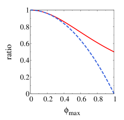
Figure 1: (Color online) The ratio of optimal efficiency at maximum power to the maximum efficiency $\frac{\phi_{opt}(\dot{W}_{max})}{\phi_{max}}$ (solid curve) and the ratio of the power at maximum efficiency to the maximum power $\frac{\dot{W}(\phi_{max})}{\dot{W}_{max}}$ (dashed curve) as functions of the maximum efficiency $\phi_{max}$, as given by Eq. (21), for thermodynamic machines with symmetric Onsager matrix.

We remark that the largest eigenvalue of $\hat{{\cal M}}_{II}^{-1/2}\hat{{\cal M}}_{IO}\hat{{\cal M}}_{OO}^{-1}\hat{{\cal M}}_{OI}\hat{{\cal M}}_{II}^{-1/2}$ is the same as the largest eigenvalue of $\hat{{\cal M}}_{OO}^{-1/2}\hat{{\cal M}}_{OI}\hat{{\cal M}}_{II}^{-1}\hat{{\cal M}}_{IO}\hat{{\cal M}}_{OO}^{-1/2}$ (proof is given in Appendix B). Particularly in thermoelectric energy conversion, this means that the figures of merit for the engine, refrigerator, and heat pump are the same. These properties can be used to simplify the calculation of the figure of merit when one of the two is easier to calculate.

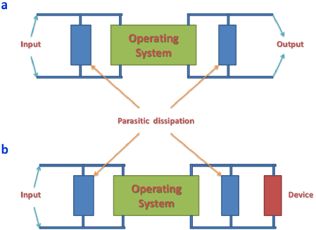
Figure 2: (Color online) Schematic of realistic thermodynamic machines. A machine accepts input energy and convert it into output energy. The output can be assigned to a huge reservoir (e.g., an electrical power grid with huge capacity) (a), or to a finite device (b). In realistic situations there are mechanisms that dissipate part of input energy and prevent it from been converted into useful outputs, as well as mechanisms that consumes part of output energy and reduce the amount of useful outputs. These mechanisms are called “parasitic dissipation”.

IV Realistic considerations: output to a huge reservoir or to a finite device

In realistic situations the input energy may pass through some parallel channels without entering into the system which reduces the amount of useful input energy. Besides, the output energy can also be dissipated into channels parallel to the device accepting the output power. These mechanisms are called as “parasitic dissipation”. The effect is described by the following phenomenological equations

$$\vec{{\cal J}}_{I}^{p}=\hat{{\cal M}}_{II}^{p}\vec{{\cal F}}_{I},\quad\quad\vec{{\cal J}}_{O}^{p}=\hat{{\cal M}}_{OO}^{p}\vec{{\cal F}}_{O}.$$ (22)

Here the superscript $p$ stands for parasitic dissipation. The currents for energy input into the operating system becomes $\vec{{\cal J}}_{I}+\vec{{\cal J}}_{I}^{p}$. And the currents that load into the device becomes $\vec{{\cal J}}_{O}+\vec{{\cal J}}_{O}^{p}$. The equivalent circuit is depicted in Fig. 2. Taking into account of those parasitic currents modifies the response coefficients as

$$\hat{{\cal M}}_{II}\to\hat{{\cal M}}_{II}+\hat{{\cal M}}_{II}^{p},\quad\hat{{\cal M}}_{OO}\to\hat{{\cal M}}_{OO}+\hat{{\cal M}}_{OO}^{p}.$$ (23)

Parasitic dissipation increases the eigenvalues of the matrices $\hat{{\cal M}}_{II}$ and $\hat{{\cal M}}_{OO}$ because both $\hat{{\cal M}}_{II}^{p}$ and $\hat{{\cal M}}_{OO}^{p}$ are positive matrices. As a consequence the degree of coupling $\lambda$ and the figure of merit $\xi$ are reduced, according to Eqs. (15) and (16). This is consistent with the physical picture that part of the useful energy is consumed by the parasitic dissipation.

Energy from the operating system can be outputted to (i) a huge reservoir (e.g., a power grid with huge capacity), or to (ii) a finite device. The optimization presented in Sec. III is for option (i) where the output current $\vec{{\cal J}}_{O}$ does not induce any observable effect on the huge reservoir which in turn modifies the force $\vec{{\cal F}}_{O}$, so that $\vec{{\cal J}}_{O}$ and $\vec{{\cal F}}_{O}$ are uncorrelated. In electrical circuit analog, it is equivalent to using the output energy to charge a huge capacitor where the charging current $\vec{{\cal J}}_{O}$ does not change the voltage across the capacitor $\vec{{\cal F}}_{O}$. For option (ii) if the response of the device is $\vec{{\cal J}}_{O}^{L}=\hat{{\cal M}}_{L}\vec{{\cal F}}_{O}$, the Kirchhoff’s current law requires that $\vec{{\cal J}}_{O}+\vec{{\cal J}}_{O}^{L}=0$. Therefore,

$$\vec{{\cal F}}_{O}=-(\hat{{\cal M}}_{OO}+\hat{{\cal M}}_{L})^{-1}\hat{{\cal M}}_{OI}\vec{{\cal F}}_{I}.$$ (24)

The power consumed by the device is

$$\vec{{\cal F}}_{O}^{T}\hat{{\cal M}}_{L}\vec{{\cal F}}_{O} = \vec{{\cal F}}_{I}^{T}\hat{{\cal M}}_{IO}(\hat{{\cal M}}_{OO}+\hat{{\cal M}}_{L})^{-1}\hat{{\cal M}}_{L}$$ (25)

$$\ \ \times(\hat{{\cal M}}_{OO}+\hat{{\cal M}}_{L})^{-1}\hat{{\cal M}}_{OI}\vec{{\cal F}}_{I}.$$

The input exergy is

$$\vec{{\cal F}}_{I}^{T}\vec{{\cal J}}_{I}=\vec{{\cal F}}_{I}^{T}(\hat{{\cal M}}_{II}-\hat{{\cal M}}_{IO}(\hat{{\cal M}}_{OO}+\hat{{\cal M}}_{L})^{-1}\hat{{\cal M}}_{OI})\vec{{\cal F}}_{I}.$$ (26)

The exergy efficiency is then

$$\phi=\frac{\vec{{\cal F}}_{O}^{T}\hat{{\cal M}}_{L}\vec{{\cal F}}_{O}}{\vec{{\cal F}}_{I}^{T}\vec{{\cal J}}_{I}}.$$ (27)

By varying $\hat{{\cal M}}_{L}$ of the device that receives power from the operating system, we find that the maximum output power is reached at

$$\hat{{\cal M}}_{L}=\hat{{\cal M}}_{OO},$$ (28)

whereas the maximum exergy efficiency is reached when

$$\hat{{\cal M}}_{L}=\sqrt{1-\lambda}\hat{{\cal M}}_{OO}.$$ (29)

At these conditions we obtain again Eqs. (16), (18), (19), and (20). The above results reflect the importance of matching between the response of the device $\hat{{\cal M}}_{L}$ and that of the system $\hat{{\cal M}}_{OO}$ in optimizing the efficiency and output powerimp-match . Particularly, Eq. (28) generalizes the maximum power theorem (Jacobi’s Law for electrical circuits, i.e., “Maximum power is transferred when the internal resistance of the source equals the resistance of the load, when the external resistance can be varied, and the internal resistance is constant”) to all thermodynamic machines with symmetric Onsager matrix in the linear-response regime.

There are two possible schemes of adjusting the input forces, $\vec{{\cal F}}_{I}$, to optimize the performance of the machine. The first scheme is to optimize the efficiency, i.e., to optimize $\lambda$. This has been discussed in Sec. III. This scheme reflects balance between optimizing output power and efficiency which is relevant to some biological and ecological systemsodum . The second scheme is to adjust $\vec{{\cal F}}_{I}$ for further optimization of the output power. This will lead to efficiency smaller or equal to that in Eq. (19). Hence the exergy efficiency for this scheme is also not larger than 50%. From Eqs. (15) and (20) one finds that $\dot{W}_{max}=\frac{1}{4}\vec{{\cal F}}_{I}^{T}\hat{{\cal M}}_{IO}\hat{{\cal M}}_{OO}^{-1}\hat{{\cal M}}_{OI}\vec{{\cal F}}_{I}$. The above can be optimized to be $\dot{W}_{max}=\frac{1}{4}\Upsilon\left(\vec{{\cal F}}_{I}^{T}\vec{{\cal F}}_{I}\right)$, with $\Upsilon$ being the largest eigenvalue of the matrix $\hat{{\cal M}}_{IO}\hat{{\cal M}}_{OO}^{-1}\hat{{\cal M}}_{OI}$. It can be shown that $\Upsilon$ is positive [see Appendix B]. There is no obvious upper bound on it that is imposed by the laws of thermodynamics (except maybe in the zero temperature limitjoe ). The above derivation is meaningful only when all input thermodynamic forces ${\cal F}_{n}$ ($\forall n\in I$) are measured in the same physical unit and scale. This requirement is usually not satisfied for systems with more than one type of input forces (e.g., if both mechanical and electrical forces are used for energy input). Discussion on this scheme of performance optimization depends on specific systems which is of little interest for our purpose.

V optimal exergy efficiency and power for systems with asymmetric Onsager matrix

We now study systems with asymmetric Onsager matrix. We first note that $\vec{{\cal F}}_{I}^{T}\hat{{\cal M}}_{II}\vec{{\cal F}}_{I}={\cal F}_{I}^{T}\hat{{\cal M}}^{s}_{II}\vec{{\cal F}}_{I}$ and $\vec{{\cal F}}_{O}^{T}\hat{{\cal M}}_{OO}{\cal F}_{O}=\vec{{\cal F}}_{O}^{T}\hat{{\cal M}}^{s}_{OO}\vec{{\cal F}}_{O}$ where $\hat{{\cal M}}^{s}_{II}=\frac{1}{2}\left(\hat{{\cal M}}_{II}+\hat{{\cal M}}^{T}_{II}\right)$ and $\hat{{\cal M}}^{s}_{OO}=\frac{1}{2}\left(\hat{{\cal M}}_{OO}+\hat{{\cal M}}^{T}_{OO}\right)$. This property is due to the symmetry of the summation over indices of forces.

It is hard to derive the optimal exergy efficiency and power for general systems with asymmetric Onsager matrix (see Appendix C). Here we focus on a special situation where $\hat{{\cal M}}_{OI}=r\hat{{\cal M}}_{IO}^{T}$ with $r$ being a real number. Such a simplification is for the convenience of treatment instead of inspired by realistic physical systems. For this particular situation, from Eq. (11), we find $\vec{{\cal F}}_{O}=-\frac{1+r^{-1}\phi_{max}}{2}\left(\hat{{\cal M}}_{OO}^{s}\right)^{-1}\hat{{\cal M}}_{OI}\vec{{\cal F}}_{I}$. Inserting this into Eq. (1) and solving the equation for $\phi_{max}$, we obtain

$$\phi_{max}=r\frac{\sqrt{\xi+1}-1}{\sqrt{\xi+1}+1}$$ (30)

where $\xi$ is given by the same expression as in Eqs. (16) and (17) but with $\hat{{\cal M}}_{OO}$ and $\hat{{\cal M}}_{II}$ replaced by their symmetric counterparts $\hat{{\cal M}}_{OO}^{s}$ and $\hat{{\cal M}}_{II}^{s}$. The exergy efficiency for maximum power is given by

$$\phi_{opt}(\dot{W}_{max})=\frac{r\xi}{2(\xi+2)}.$$ (31)

From the second law of thermodynamics the restriction on $\lambda$ is [see Appendix B]

$$\frac{4r}{(1+r)^{2}}\leq\lambda<0,\quad{\rm if}\quad r<0,$$ (32a)

$$0\leq\lambda\leq\frac{4r}{(1+r)^{2}},\quad{\rm if}\quad r\geq 0.$$ (32b)

The above restrictions give rise to $\xi+1=\frac{1}{1-\lambda}\geq 0$ and $r(\sqrt{\xi+1}-1)>0$, so that the optimal exergy efficiency given in Eq. (30) is positive and well-defined.

The maximum possible, i.e., the upper bound of exergy efficiency is reached at $\lambda=\frac{4r}{(1+r)^{2}}$ as

$$\phi_{bound}=r^{2},\quad{\rm if}\quad|r|<1,$$ (33a)

$$\phi_{bound}=1,\quad{\rm if}\quad|r|\geq 1.$$ (33b)

The dissipation at the upper bound exergy efficiency is

$$T\dot{S}_{tot}=(1-r)^{2}\left(\vec{{\cal F}}_{I}^{T}\hat{{\cal M}}_{II}^{s}\vec{{\cal F}}_{I}\right),\quad{\rm if}\quad|r|<1,$$ (34a)

$$T\dot{S}_{tot}=0,\hskip 102.43008pt{\rm if}\quad|r|\geq 1.$$ (34b)

The entropy production for $|r|<1$ is always positive hence the upper bound efficiency is not 100%.

The upper bound of the exergy efficiency for maximum power is also reached at $\lambda=\frac{4r}{(1+r)^{2}}$ with

$$\left.\phi_{opt}(\dot{W}_{max})\right|_{bound}=\frac{r^{2}}{r^{2}+1}.$$ (35)

From the above equation the Curzon-Ahlborn limit of exergy efficiencyca ; ca-ex ; Seifert-review $\phi_{CA}=50\%$ can be overcome when $|r|>1$. This is first pointed out by Benenti et al. in the study of thermoelectric efficiency in systems with broken time-reversal symmetrytrb1 .

The output power at maximum exergy efficiency is

$$\dot{W}(\phi_{max})=\frac{1}{4}(1-r^{-2}\phi_{max}^{2})r\lambda\left(\vec{{\cal F}}_{I}^{T}\hat{{\cal M}}_{II}^{s}\vec{{\cal F}}_{I}\right).$$ (36)

Combining the above with Eq. (33), the upper bound of efficiency for $|r|<1$ is $\phi=r^{2}$ so that the output power is positive. For $|r|>1$ the maximum efficiency can reach 100% without conflicting the requirement of positive output power. The maximum output power is

$$\dot{W}_{max}=\frac{1}{4}r\lambda\left(\vec{{\cal F}}_{I}^{T}\hat{{\cal M}}_{II}^{s}\vec{{\cal F}}_{I}\right).$$ (37)

We find that

$$\frac{\phi_{max}}{\phi_{opt}(\dot{W}_{max})}=1+r^{-2}\phi_{max}^{2},$$ (38a)

$$\frac{\dot{W}(\phi_{max})}{\dot{W}_{max}}=1-r^{-2}\phi_{max}^{2}.$$ (38b)

Eqs. (33b) and (38b) reveal that for systems with asymmetric Onsager matrix with $|r|>1$, the output power is nonzero even when $\phi_{max}$ reaches the value of 100% in the reversible limit. These results agree with the findings of Benenti et al. on thermoelectric efficiency and power in time-reversal symmetry broken systemstrb1 .

It is interesting to study the optimal exergy efficiency and power of the reversed machine (i.e., the machine with output input reversed). The output power of the reversed machine is $-\vec{{\cal F}}_{I}^{T}\vec{{\cal J}}_{I}=-\dot{\cal A}_{in}$, while the input power becomes $\vec{{\cal F}}_{O}^{T}\vec{{\cal J}}_{O}=-\dot{\cal A}_{out}$. The reversed machine is working in the region with $\dot{\cal A}_{I}<0$. The efficiency of the reversed machine is defined as

$$\phi^{\prime}=\frac{\dot{\cal A}_{in}}{\dot{\cal A}_{out}}.$$ (39)

We find that the optimal exergy efficiency and powers are similar but with $r$ replaced by $r^{-1}$. Therefore for $|r|>1$ the reversed machine can not reach the efficiency of 100%, whereas for $|r|<1$ the reversed machine can have 100% efficiency with finite power.

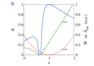
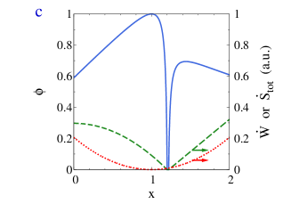
Figure 3: (Color online) The exergy efficiency $\phi$ (solid curves), output power $\dot{W}$ (dashed curves), and total entropy production $\dot{S}_{tot}$ (dotted curves) as functions of $x$ for $r=1$ (a), $r=0.6$ (b), and $r=1.2$ (c). For each figure the left region with positive efficiency is the operating region of the machine, while the right region with positive efficiency is the operating region for the reversed machine. The definitions of efficiency and output power are different for the machine and the reversed machine.

To demonstrate this we plot the efficiency as a function of $x$ for $\vec{{\cal F}}_{O}=-\frac{r+x}{2r}\left(\hat{{\cal M}}_{OO}^{s}\right)^{-1}\hat{{\cal M}}_{OI}\vec{{\cal F}}_{I}$ in Fig. 3. At the limit with $\lambda=\frac{4r}{(1+r)^{2}}$ the efficiency is

$$\phi=\frac{r^{2}-x^{2}}{1+r^{2}-2x}.$$ (40)

The output power $\dot{W}=\frac{r^{2}-x^{2}}{(1+r)^{2}}(\vec{{\cal F}}_{I}^{T}\hat{{\cal M}}_{II}^{s}\vec{{\cal F}}_{I})$ is positive when $|x|<|r|$. If $x>(1+r^{2})/2$, both the input and output exergy are negative which indicates that the machine is operating at the reversed mode. The efficiency of the reversed machine is then

$$\phi^{\prime}=\frac{2x-1-r^{2}}{x^{2}-r^{2}}$$ (41)

The output power is $\dot{W}=\frac{2x-1-r^{2}}{(1+r)^{2}}(\vec{{\cal F}}_{I}^{T}\hat{{\cal M}}_{II}^{s}\vec{{\cal F}}_{I})$.

For all values of $r$ the reversible limit $T\dot{S}_{tot}=0$ is reached at $x=1$. When $r=1$, 100% efficiency is reached by both the machine and the reversed machine at $x=1$ where the input and output exergy as well as entropy production vanish [see Fig. 3a]low-diss . For $|r|<1$, the machine cannot reach to 100% efficiency, but the reversed machine can reach 100% efficiency with finite output power, because at $x=1$ the machine is operating in the reversed mode [see Fig. 3b]. For $|r|>1$, the output power of the machine is positive at $x=1$, thus the machine can reach 100% efficiency with finite output power [see Fig. 3c].

In systems with broken time-reversal symmetry, such as two-dimensional electron systems under perpendicular magnetic field, Hall effect, and Nernst-Ettingshausen effect give rise to asymmetric Onsager matrixchien ; trb3 . The asymmetric Onsager matrix can be decomposed into the symmetric part and anti-symmetric part. Specifically,

$$\hat{{\cal M}}_{IO}=\hat{{\cal M}}_{IO}^{s}+\hat{{\cal M}}_{IO}^{a},\quad\hat{{\cal M}}_{OI}=\hat{{\cal M}}_{OI}^{s}+\hat{{\cal M}}_{OI}^{a}$$ (42)

with $\hat{{\cal M}}_{IO}^{s}=(\hat{{\cal M}}_{OI}^{s})^{T}$ and $\hat{{\cal M}}_{IO}^{a}=-(\hat{{\cal M}}_{OI}^{a})^{T}$. The symmetric part, $\hat{{\cal M}}_{IO}^{s}$, is related to entropy production and is restricted by the second law of thermodynamics. The anti-symmetric part, $\hat{{\cal M}}_{IO}^{a}$, however, does not contribute to dissipation and is often related to Berry phase effectsniu . The output and input exergy can be written as

$$\dot{\cal A}_{out}=\dot{\cal A}_{out}^{s}-\vec{{\cal F}}_{O}^{T}\hat{{\cal M}}_{OI}^{a}\vec{{\cal F}}_{I},\quad\dot{\cal A}_{in}=\dot{\cal A}_{in}^{s}-\vec{{\cal F}}_{O}^{T}\hat{{\cal M}}_{OI}^{a}\vec{{\cal F}}_{I}$$ (43)

where $\dot{\cal A}_{out}^{s}$ and $\dot{\cal A}_{in}^{s}$ are the output and input exergy for the symmetrized Onsager matrix with

$$\dot{\cal A}_{out}^{s}=-\vec{{\cal F}}_{O}^{T}\hat{{\cal M}}_{OI}^{s}\vec{{\cal F}}_{I}-\vec{{\cal F}}_{O}^{T}\hat{{\cal M}}_{OO}^{s}\vec{{\cal F}}_{O},$$

$$\dot{\cal A}_{in}^{s}=\vec{{\cal F}}_{I}^{T}\hat{{\cal M}}_{IO}^{s}\vec{{\cal F}}_{O}+\vec{{\cal F}}_{I}^{T}\hat{{\cal M}}_{II}^{s}\vec{{\cal F}}_{I}.$$

The additional term in Eq. (43), $\vec{{\cal F}}_{O}^{T}\hat{{\cal M}}_{OI}^{a}\vec{{\cal F}}_{I}$, does not cause entropy production, but shift the input and output powers by the same magnitude. In this way the reversible limit is shifted from the boundary between the machine and the reversed machine, into the operating region of the machine or the reversed machine, whichever has positive output power in such limit.

It should be emphasized here that although potential advantages of systems with asymmetric Onsager matrix have been predicted by Benenti et al.trb1 from phenomenological theory (and extended in this work), no realistic physical system has been shown to have finite power at 100% efficiencytrb2 ; trb3 . It is very important to study efficiency and power of realistic physical systems with asymmetric Onsager matrix to clarify whether breaking time reversal symmetry could indeed improve the performance of a thermodynamic machinetrb2 ; trb3 .

VI Application to realistic systems

VI.1 Example I: Thermoelectric energy conversion in isotropic systems

Thermoelectric transport equation for an isotropic system is given by

$$\left(\begin{array}[]{c}\vec{j}\\ \vec{j}_{q}\end{array}\right)=\left(\begin{array}[]{cccc}\sigma{\hat{\mathbf{1}}}&\sigma ST{\hat{\mathbf{1}}}\\ \sigma ST{\hat{\mathbf{1}}}&(\kappa T+\sigma S^{2}T^{2}){\hat{\mathbf{1}}}\end{array}\right)\left(\begin{array}[]{c}\vec{{\cal E}}\\ -\vec{\mbox{\boldmath$\nabla$\unboldmath}}T/T\end{array}\right),$$ (44)

where the electric field $\vec{{\cal E}}$ include both the external and induced electric fields. Here $\sigma$ is the electrical conductivity, $S$ is the Seebeck coefficient, $\kappa$ the thermal conductivity, and $\hat{\mathbf{1}}$ is the $3\times 3$ identity matrix. The efficiency, or coefficient of performance, of a thermoelectric refrigerator is

$$\eta\equiv\frac{\dot{Q}}{\dot{W}}=\frac{T}{\Delta T}\frac{\vec{j}_{q}\cdot\vec{\mbox{\boldmath$\nabla$\unboldmath}}T/T}{\vec{j}\cdot\vec{{\cal E}}}=\eta_{C}\phi,\quad\eta_{C}\equiv\frac{T}{\Delta T}.$$ (45)

For a slab of thickness $\ell_{z}$ with temperature gradient and electric field along the direction $z$ which is perpendicular to the slab plane, the temperature difference is $\Delta T=-\ell_{z}\frac{dT}{dz}>0$ for $\frac{dT}{dz}<0$. The maximum coefficient of performance $\eta_{max}$ is related to the maximum exergy efficiency by

$$\eta_{max}=\eta_{C}\phi_{max}=\eta_{C}\frac{\sqrt{\xi+1}-1}{\sqrt{\xi+1}+1}.$$ (46)

The figure of merit is related to the degree of coupling which, according to Eq. (17), is the largest eigenvalue of the following coupling matrix

$$\hat{\Lambda}=\frac{(\sigma ST)^{2}}{\sigma(\kappa T+\sigma S^{2}T^{2})}\hat{\mathbf{1}}.$$ (47)

Since $\hat{\Lambda}$ is proportional to an identity matrix, the largest eigenvalue is just

$$\lambda=\frac{\sigma S^{2}T}{\kappa+\sigma S^{2}T}.$$ (48)

Therefore the figure of merit is

$$\xi=\frac{\lambda}{1-\lambda}=\frac{\sigma S^{2}T}{\kappa},$$ (49)

which recovers the well-known thermoelectric figure of merit as found by Ioffe.

VI.2 Example II: Spin-thermoelectric effect

In conducting magnetic materials charge, spin, and thermal transports are coupled together. There couplings are called spin-thermoelectric or spin-caloric effectbauer . In isotropic materials spin-thermoelectric effect is described by the following transport equationbauer

$$\left(\begin{array}[]{c}\vec{j}\\ \vec{j}_{s}\\ \vec{j}_{q}\end{array}\right)=\left(\begin{array}[]{cccc}\sigma{\hat{\mathbf{1}}}&\sigma P{\hat{\mathbf{1}}}&\sigma ST{\hat{\mathbf{1}}}\\ \sigma P{\hat{\mathbf{1}}}&\sigma{\hat{\mathbf{1}}}&P^{\prime}\sigma ST{\hat{\mathbf{1}}}\\ \sigma ST{\hat{\mathbf{1}}}&P^{\prime}\sigma ST{\hat{\mathbf{1}}}&\kappa_{0}T{\hat{\mathbf{1}}}\end{array}\right)\left(\begin{array}[]{c}\vec{{\cal E}}\\ -\vec{\mbox{\boldmath$\nabla$\unboldmath}}m\\ -\vec{\mbox{\boldmath$\nabla$\unboldmath}}T/T\end{array}\right).$$ (50)

where $\vec{j}={\vec{j}}^{(\uparrow)}+{\vec{j}}^{(\downarrow)}$, $\vec{j}_{s}={\vec{j}}^{(\uparrow)}-{\vec{j}}^{(\downarrow)}$ with ${\vec{j}}^{(\uparrow)}$ and ${\vec{j}}^{(\downarrow)}$ denoting the electrical currents of the spin-up and spin-down electrons, respectively. $\vec{{\cal E}}=-\vec{\mbox{\boldmath$\nabla$\unboldmath}}\mu/e$ with $\mu\equiv(\mu_{\uparrow}+\mu_{\downarrow})/2$, and $m\equiv(\mu_{\uparrow}-\mu_{\downarrow})/(2e)$ where $\mu_{\uparrow}$ and $\mu_{\downarrow}$ are the electrochemical potentials for spin-up and spin-down electrons, respectively, $e$ is the carrier charge. $\sigma$ is the electrical conductivity, $S$ is the Seebeck coefficient, $P$ and $P^{\prime}$ are two dimensionless quantities describing spin polarization of carriers in different transport channels, $\kappa_{0}$ is the heat conductivity at $\vec{{\cal E}}=\vec{\mbox{\boldmath$\nabla$\unboldmath}}m=0$. Microscopically they are given by

$$\sigma=\int dE\left(-\frac{\partial n_{F}}{\partial E}\right)\sum_{s}\sigma^{(s)}(E),$$ (51a)

$$P=\langle s_{z}\rangle,\quad S=\frac{\langle E\rangle}{eT},$$ (51b)

$$P^{\prime}=\frac{\langle Es_{z}\rangle}{\langle E\rangle},\quad\kappa_{0}T=e^{-2}\sigma\langle E^{2}\rangle.$$ (51c)

with $\sigma^{(s)}(E)$ ($s=\uparrow,\downarrow$) being spin- and energy-dependent conductivity. We have set the energy zero to be at the (equilibrium) chemical potential, i.e., $\mu\equiv 0$. $s_{z}=1$ or -1 for spin up and down, respectively. $n_{F}=1/[\exp(\frac{E}{k_{B}T})+1]$ is the Fermi distribution of the carrier. The averages in the above equations are defined as

$$\langle{\cal O}\rangle\equiv\sigma^{-1}\int dE\left(-\frac{\partial n_{F}}{\partial E}\right)\sum_{s}\sigma^{(s)}(E){\cal O}.$$ (52)

The above equations can be viewed as Mott relationsMC generalized to spin-dependent transport. It assumes elastic transport (by which the energy dependent conductivity is well-defined) and fails when inelastic transport processes become important as pointed out by the author and collaboratorsourworks .

We consider refrigeration driven by both the electric field $\vec{{\cal E}}$ and the spin density gradient $\vec{\mbox{\boldmath$\nabla$\unboldmath}}m$. The coefficient of performance of the refrigerator is defined as

$$\eta\equiv\frac{\dot{Q}}{\dot{W}}=\frac{T}{\Delta T}\frac{\vec{j}_{q}\cdot\vec{\mbox{\boldmath$\nabla$\unboldmath}}T/T}{\vec{j}\cdot\vec{{\cal E}}-\vec{j}_{s}\cdot\vec{\mbox{\boldmath$\nabla$\unboldmath}}m}=\eta_{C}\phi,\quad\eta_{C}=\frac{T}{\Delta T}.$$ (53)

Schematic of spin-thermoelectric cooling is shown in Fig. 4. Consider a slab of thickness $\ell_{z}$ where the temperature gradient, electric field, and spin density gradient are along the direction perpendicular to the slab plane, i.e., the $z$ direction. The temperature difference is $\Delta T=-\ell_{z}\frac{dT}{dz}>0$ for $\frac{dT}{dz}<0$. The maximum coefficient of performance is again related to the maximum exergy efficiency as given in Eq. (46). Using Eqs. (16) and (50) we obtain

$$\xi=\frac{\sigma TS^{2}(1-2PP^{\prime}+P^{\prime 2})}{\kappa_{0}(1-P^{2})-\sigma TS^{2}(1-2PP^{\prime}+P^{\prime 2})}.$$ (54)

Remarkably one can show that the above degree of coupling is greater than the figure of merit for thermoelectric cooling,

$$\xi_{TE}=\frac{\sigma TS^{2}}{\kappa_{0}-\sigma TS^{2}},$$ (55)

and the figure of merit for spin-Peltier coolingbauer ; sp ,

$$\xi_{SP}=\frac{\sigma TS^{2}P^{\prime 2}}{\kappa_{0}-\sigma TS^{2}P^{\prime 2}}.$$ (56)

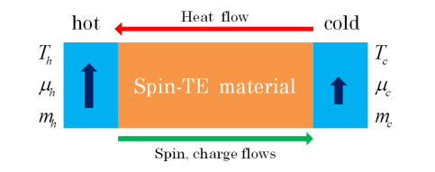
Figure 4: (Color online) Spin-thermoelectric cooling. A spin-thermoelectric (“spin-TE”) material (i.e., a conducting ferromagnetic material) sandwiched between two ferromagnetic electrodes with different temperature $T$, electrochemical potential $\mu\equiv(\mu_{\uparrow}+\mu_{\downarrow})/2$, and spin accumulation $m\equiv(\mu_{\uparrow}-\mu_{\downarrow})/(2e)$ where $\mu_{\uparrow}$ and $\mu_{\downarrow}$ are the electrochemical potentials for spin-up and spin-down electrons, respectively, and $e$ is the carrier charge. For a set-up with $T_{h}>T_{c}$, $\mu_{h}>\mu_{c}$, and $m_{h}>m_{c}$ (the subscripts $h$ and $c$ denoting the hot and cold terminals, respectively), cooling (heat flowing from the cold terminal to the hot terminal) is driven by both the charge and spin flows.

This interesting phenomenon has a geometric origin which is understood as follows. The electric field and the spin-density gradient can be parametrized as

$$\vec{{\cal E}}=\vec{{\cal F}}_{0}\cos\theta,\quad-\vec{\mbox{\boldmath$\nabla$\unboldmath}}m=\vec{{\cal F}}_{0}\sin\theta$$ (57)

where $\vec{{\cal F}}_{0}=\vec{{\bf e}}_{z}\sqrt{\frac{1}{2e^{2}}(|\vec{\mbox{\boldmath$\nabla$\unboldmath}}\mu_{\uparrow}|^{2}+|\vec{\mbox{\boldmath$\nabla$\unboldmath}}\mu_{\downarrow}|^{2})}$ with $\vec{{\bf e}}_{z}$ being the transport direction. $|\vec{{\cal F}}_{0}|$ is the total “magnitude” of the input force. The heat current,

$$\vec{j}_{q}=\vec{j}_{q0}+\vec{j}_{q1}+\vec{j}_{q2},$$ (58)

consists of three parts: thermal conduction $\vec{j}_{q0}=-\kappa_{0}\vec{\mbox{\boldmath$\nabla$\unboldmath}}T$, Peltier cooling $\vec{j}_{q1}=\sigma ST\vec{{\cal E}}$, and spin-Peltier cooling $\vec{j}_{q2}=-P^{\prime}\sigma ST\vec{\mbox{\boldmath$\nabla$\unboldmath}}m$. The cooling is achieved when the sum of the Peltier current $\vec{j}_{q1}$ and the spin-Peltier current $\vec{j}_{q2}$ exceeds the thermal conduction current $\vec{j}_{q0}$.

Tuning the angle $\theta$ changes the relative amplitude of the Peltier and spin-Peltier heat currents, $\vec{j}_{q1}$ and $\vec{j}_{q2}$. These two currents can be of the same sign, or the opposite sign, depending on $\theta$. When $\vec{j}_{q1}$ and $\vec{j}_{q2}$ have the same sign, the cooling is enhanced, leading to higher efficiency. However, when $\vec{j}_{q1}$ and $\vec{j}_{q2}$ have opposite sign, the cooling is suppressed and the efficiency is reduced. This is explicitly shown in Fig. 5. The underlying physics is more complicated when the input work $\dot{W}$ is taken into consideration as well. However, this simplified picture gives a snapshot that the two cooling mechanisms can have cooperative effects.

We also calculated the figure of merit for spin-Peltier cooling $\xi_{SP}$ as function of $P^{\prime}$ according to Eq. (56) as shown in Fig. 6a for $\sigma S^{2}T/\kappa_{0}=0.1$. For the same parameter, we plot the enhancement factor $\xi/{\rm max}(\xi_{TE},\xi_{SP})$ as function of $P$ and $P^{\prime}$ in Fig. 6b. Significant enhancement of figure of merit due to cooperative effect is attainable when $P^{\prime}$ deviates from $P$ markedly.

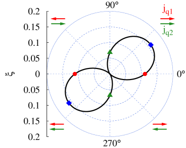
Figure 5: (Color online) Polar plot of $\xi$ vs. $\theta$. The parameters are $P=0.2$, $P^{\prime}=0.8$, $S=50$ $\mu$V/K, and $T=300$ K. The heat conductivity is $\kappa_{0}=\sigma LT$ with the Lorenz number of $L=2.5\times 10^{-8}$ W ${\rm\Omega}$ K^-2. The arrows indicates the relative direction between $\vec{j}_{q1}$ (red arrows) and $\vec{j}_{q2}$ (green arrows). The red dots represent the thermoelectric figure of merit $\xi_{TE}$, the green triangles represent the spin-Peltier figure of merit $\xi_{SP}$, and the blue rhombuses denote the figure of merit $\xi$ of combined thermoelectric and spin-Peltier cooling.

Efficient spin-thermoelectric cooling demands large Seebeck coefficient. According to the literature, large Seebeck coefficient ranging from 100 to 45000 $\mu$V/K can be attained in magnetic or strongly-correlated semiconductorsmag-sem and magnetic tunnel junctionsmtj . Sizable figure of merit, $\xi\sim 1$, however, is still to be achievedmag-sem .

The figure of merit at fixed $\theta$ is found as

$$\xi(\theta)=\frac{\sigma S^{2}T(P^{\prime}\sin\theta+\cos\theta)^{2}(1+2P\sin\theta\cos\theta)}{\kappa_{0}-\sigma S^{2}T(P^{\prime}\sin\theta+\cos\theta)^{2}(1+2P\sin\theta\cos\theta)}$$ (59)

The maximum exergy efficiency is achieved at $\theta=\theta_{M}$ with

$$\tan\theta_{M}=\frac{P^{\prime}-P}{1-P^{\prime}P}.$$ (60)

The figure of merit at $\theta=\theta_{M}$ is exactly the same as that given in Eq. (54), which is greater than the figures of merit for thermoelectric and spin-Peltier cooling, $\xi_{TE}$ and $\xi_{SP}$, unless $P=P^{\prime}$. Such cooperative effect prevails in systems with multiple cross-correlated responses, which can be exploited to improve the efficiency. The discussions here can also be applied to the efficiency and figure of merit of spin-thermoelectric power generatorstem-gen .

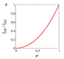
Figure 6: (Color online) (a) The ratio of the figure of merit of spin-Peltier cooling $\xi_{SP}$ to that of thermoelectric cooling $\xi_{TE}$ as a function of $P^{\prime}$. (b) The enhancement of figure of merit due to cooperative effect, $\xi/{\rm max}(\xi_{TE},\xi_{SP})$, as a function of $P$ and $P^{\prime}$. The parameters are $S=50$ $\mu$V/K and $T=300$ K. The heat conductivity is $\kappa_{0}=\sigma LT$ with the Lorenz number of $L=2.5\times 10^{-8}$ W ${\rm\Omega}$ K^-2. The white region in (b) near $P=1$ is forbidden by the second law of thermodynamics.

VI.3 Example III: Piezoelectric, piezomagnetic and magnetoelectric effects

Piezoelectric energy harvest has been studied extensively and made into useful devicespe-review . There is also the piezomagnetic effect where elastic strain induces a magnetization or vice versatem1 . These two effects are common in ferroelectric and ferromagnetic insulatorstem1 . Materials with simultaneous ferroelectric and ferromagnetic properties, or more generally multiple spontaneous electric and magnetic orderstem1 ; multi1 ; science , are called multiferroics. An important technologically property of multiferroics is the magnetoelectric effect which offers efficient conversion between electric and magnetic energy in the radio frequency regimetem1 . Wood and Austinwood suggested many possible applications of the magnetoelectric effect, among which there are transducers which convert the microwave magnetic field into microwave electric field, attenuators which are used to improve impedance matching in circuits, and ultrasensitive magnetic field sensorstem1 . Multiferroics with strong magnetoelectric response have been the aim of extensive studiestem1 . Recently, strong magnetoelectric response were found in both crystalline (such as CaMn₇O₁₂crys1 , TbMnO₃crys2 , and HoMnO₃crys3 ) and nano-composite (such as BiFeO₃ thin film heterostructurescomp1 and BaTiO₃-CoFe₂O₄ nano-structurescomp2 ) materials. In many of these materials the interplay of piezoelectric and piezomagnetic responses play an important role. In fact, multiferroics can be made from nano-composites of ferroelectric and ferromagnetic compounds where elastic strain at interfaces mediate coupling between electric and magnetic polarizationsscience ; nan .

In these materials a full description of responses to external mechanical, electric, and magnetic forces are given bynan ; tem1

$$\left(\begin{array}[]{c}\hat{S}\\ \vec{D}\\ \vec{B}\end{array}\right)=\left(\begin{array}[]{cccc}\hat{s}&\hat{d}&\hat{q}\\ \hat{d}^{T}&\hat{\epsilon}&\hat{\alpha}\\ \hat{q}^{T}&\hat{\alpha}^{T}&\hat{\mu}_{m}\end{array}\right)\left(\begin{array}[]{c}\hat{T}\\ \vec{E}\\ \vec{H}\end{array}\right).$$ (61)

where the forces are stress $\hat{T}$, electric field $\vec{E}$, and magnetic field $\vec{H}$, the currents are strain $\hat{S}$, electric displacement $\vec{D}$, and magnetic induction $\vec{B}$. Here $\vec{D}$ and $\vec{B}$ stand for the values deviate from the equilibrium ones (which could be nonzero in materials with spontaneous polarization and magnetization). The response matrix has the dimension of $12\times 12$. Specifically, $\hat{s}$ is the $6\times 6$ compliance tensor, $\hat{\epsilon}$ is the $3\times 3$ dielectric tensor, $\hat{\mu}_{m}$ is the ($3\times 3$) permeability tensor, $\hat{d}$ describes piezoelectric response, $\hat{q}$ describes piezomagnetic response, and $\hat{\alpha}$ gives magnetoelectric response.

In general the response matrix is frequency dependent. Experiments have shown resonance behavior in magnetoelectric responsereson . Without further complication of specific circuits set-up for energy conversion at finite frequenciespe1 ; pe2 , here we consider the low-frequency limit which is sufficient to demonstrate the underlying principles. Extension of study to finite frequency regimes will be achieved in future works. First, the coupling matrix for piezoelectric energy conversion is

$$\hat{\Lambda}_{pe}=\hat{\epsilon}^{-1/2}~{}\hat{d}^{T}~{}\hat{s}^{-1}~{}\hat{d}~{}\hat{\epsilon}^{-1/2},$$ (62)

which coincides with the “electromechanical coupling tensor” introduced in Ref. pe . The largest electromechanical coupling factor of a material is given by the largest eigenvalue of the coupling matrix $\hat{\Lambda}_{pe}$. Piezoelectric effect allows harvest of mechanical energy to power portable and isolated electrical systems as well as small motors which have already found applicationspe-review . Existing materials have already shown large electromechanical coupling factors, reaching to $\gtrsim 0.5$pe1 ; ryu , which allows efficient piezoelectric energy conversion. In realistic systems, additional mechanical and electrical damping reduces the efficiencype1 ; pe2 . Although further complication must be considered for a finite frequency set-up with a mechanical oscillator, the efficiency is still an increasing function of the electromechanical coupling factorpe1 ; pe2 . Piezomagnetic effect can be used for magnetic field sensing, stress sensing, and mechanical generation of spin-wavestem1 . The coupling matrix for piezomagnetic energy conversion is

$$\hat{\Lambda}_{pm}=\hat{\mu}_{m}^{-1/2}~{}\hat{q}^{T}~{}\hat{s}^{-1}~{}\hat{q}~{}\hat{\mu}_{m}^{-1/2}.$$ (63)

The largest piezomagnetic coupling factor is the largest eigenvalue of the above matrix. Piezomagnetic coupling factor can be as large as 0.5 as welldong . The coupling matrix for magnetoelectric energy conversion is

$$\hat{\Lambda}_{em}=\hat{\mu}_{m}^{-1/2}~{}\hat{\alpha}^{T}~{}\hat{\epsilon}^{-1}~{}\hat{\alpha}~{}\hat{\mu}_{m}^{-1/2}.$$ (64)

Experiments on laminated composites of rare-earth-iron alloys (Terfenol-D) and lead-zirconate-titanate (PZT) achieved a magnetoelectric coefficient along the stacking direction as high as $\alpha_{E}=\alpha/\epsilon=$10 V cm^-1 Oe^-1ryu . Along this direction the relative dielectric constant is about 1000ryu and the relative permeability is about 4nan2 . According to these parameters, the magnetoelectric coupling factor along the stacking direction is around 0.1. The largest magnetoelectric coupling factor is given by the largest eigenvalue of the matrix $\hat{\Lambda}_{em}$.

The system also allows multiple input or output energy forms. For example, magnetic energy can be generated by simultaneously inputting electric and mechanic energy. This yield the coupling matrix of

$$\hat{\Lambda}_{m-pe}=\hat{\mu}_{m}^{-1/2}~{}\hat{q}_{pe}^{T}~{}\hat{h}_{pe}^{-1}~{}\hat{q}_{pe}~{}\hat{\mu}_{m}^{-1/2}$$ (65)

where

$$\hat{q}_{pe}=\left(\begin{array}[]{c}\hat{q}\\ \hat{\alpha}\end{array}\right),\quad\hat{h}_{pe}=\left(\begin{array}[]{cccc}\hat{s}&\hat{d}\\ \hat{d}^{T}&\hat{\epsilon}\end{array}\right).$$ (66)

Similar to the results in Sec. VI.2, cooperative effect will lead to larger degree of coupling from the above coupling matrix. That is, the exergy efficiency is no less than those of piezomagnetic effect and magnetoelectric effect. Significant improvement of efficiency could be possible by the synergetic effect in systems with cross-correlated piezo-electric-magnetic effect.

VI.4 Example IV: Biological energy conversion

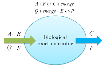
Figure 7: (Color online) Energy conversion in biological reaction. Biological reactions, $A+B\leftrightarrow C+energy$ and $Q+energy+E\leftrightarrow P$, take place in the reaction center. The first reaction produces energy which is stored in material $P$ via the second reaction. At steady states there are continuous flows of materials across the membrane of the reaction center to facilitate continuous reactions. The membrane keeps a density (chemical potential) difference between the reaction center and the outside to control reaction rates. Arrows in the figure indicate possible flows of materials when energy is produced and stored in $P$.

Biological processes are driven by various energies: the internal energy produced by oxidation and external energy from environments. Understanding of bioenergetics is one of the most important and challenging task in biology. Many of the processes can be described by Onsager’s linear-response theory (although many others cannot)caplan1 ; caplan2 ; bio1 ; bio2 ; bio3 . One example is transport across a membrane. The flows of various ions, such as Na⁺, Ca²⁺, and H⁺ as well as other materials, such as phosphorylation, oxygen, and sugars are all driven by their density gradients, chemical reaction and other forcesbio . If, e.g., some of these materials involve in a chemical reaction, flows of those materials will be correlated. Synergetic effects will appear as multiple flows take place in coorperative ways. Biological systems, may also utilize the cross-correlation of those flows to optimize energy efficiency. There have been a lot of studies of bioenergetics using irreversible thermodynamicsbio1 ; bio2 ; bio3 ; caplan1 ; caplan2 . However, none of them have reached a simple analytic results as obtained in this work.

To demonstrate the usefulness of the theory, we consider a toy model describes the reaction of

$$A+B\leftrightarrow C+energy,\quad Q+energy+E\leftrightarrow P$$ (67)

in a reaction center surrounded by a membrane. We assume the reactions are reversible with the help of enzymes. In the former reaction $A$ and $B$ are consumed to produce $C$ while some energy is generated which is absorbed by $Q$ and $E$ to form $P$ (energy stored in $P$). We assume that all energy generated in the former reaction is absorbed by the latter one. To describe such a reaction, we use six flows, $J_{A}$, $J_{B}$, $J_{Q}$, and $J_{E}$ to describe the rate of consumption of $A$, $B$, $Q$, and $E$, $-J_{C}$ and $-J_{P}$ to describe the rate of production of $C$ and $P$. The flow and reaction is illustrated in Fig. 7. The reaction is described by Eq. (9) in linear-response regime with

$$\vec{\cal J}_{I}=({\cal J}_{A},{\cal J}_{B},{\cal J}_{Q},{\cal J}_{E})^{T},\quad\vec{\cal J}_{O}=({\cal J}_{C},{\cal J}_{P})^{T},$$ (68a)

$$\vec{\cal F}_{I}=({\cal F}_{A},{\cal F}_{B},{\cal F}_{Q},{\cal F}_{E})^{T},\quad\vec{\cal F}_{O}=({\cal F}_{C},{\cal F}_{P})^{T}.$$ (68b)

The forces can be written as ${\cal F}_{i}=\delta\mu_{i}+a_{i}$ where $\delta\mu_{i}=\mu_{i}^{out}-\mu_{i}^{in}$ with $\mu_{i}^{out}$ and $\mu_{i}^{in}$ being the chemical potential of $i$ outside and inside the reaction center, respectively, $a_{i}$ is the affinity of material $i$ for the reaction which is the free energy of $i$ per mole (if ${\cal J}_{i}$ is measured in unit of mole per second). Biological systems can control those flows and their correlations through chemical reaction processes (e.g., via enzymes) as well as selective and tunable transmission of materials through the membrane. The efficiency of the biological reaction is $\phi=-\vec{\cal F}_{O}^{T}\vec{\cal J}_{O}/(\vec{\cal F}_{I}^{T}\vec{\cal J}_{I})$. The optimal efficiency is then given by Eq. (16) where the degree of coupling is given by the largest eigenvalue of the coupling matrix $\hat{\Lambda}$ given by Eq. (15). This result is much simpler than that discussed in Ref. caplan2 .

VII Conclusion and discussions

We examined the important question of “what is the maximum efficiency of a thermodynamic machine when its linear responses to the external is given?”. This question has been answered in simple limits with two thermodynamic currents. It becomes rather difficult to answer for a thermodynamic machine with arbitrarily complex responses. Efforts on the problem in the literature failed in yielding general and analytic results that are useful for material and structure engineering in advanced energy technologies. Pushed by fast developing nanotechnology and material technologies, complex systems with advanced functions play more and more important roles. It becomes increasingly demanded to extend the known, simple results on efficiency optimization with two thermodynamic currents to those complex systems which is characterized by a $N\times N$ Onsager matrix ($N>2$).

We derived the optimal efficiency and powers for general thermodynamic machines with arbitrary linear-response coefficients. The results are written in simple and analytic forms. Based on those results we establish two general relationships between the optimal efficiency and powers for two realistic optimization schemes: (i) maximum efficiency and (ii) optimal efficiency for maximum power. We proved that the upper bound efficiency at maximum output power is 50% for all thermodynamic systems with symmetric Onsager response matrix. The results are confirmed by considering realistic energy systems where the output power is consumed by a device of which the response coefficients can be varied. We proved that the maximum output power is reached when the response matrix of the device receiving the power, $\hat{{\cal M}}_{L}$, is equal to that of the power-supplying machine in the output sector, $\hat{{\cal M}}_{OO}$. This proof generalizes the maximum power theorem (Jacobi’s Law) to all thermodynamic machines with symmetric Onsager matrix in the linear-response regime. We also extend the studies to systems with asymmetric Onsager matrix (for a particular class of systems) where the efficiency at maximum output power can exceed 50%. Besides, in such systems the second law of thermodynamics does not forbid the reversible limit of efficiency, 100%, to be reached at finite output power. This phenomenon is caused by redistribution of free energy between the input and output channels induced by dissipationless responses (e.g., by magnetic field, geometric phases, etc). We also show that such limit can only be reached in a machine by its normal mode or reversed mode, but not by both of them.

Several examples are presented to demonstrate applications of the theory. First for isotropic thermoelectric systems, we recover Ioffe’s well-known results. We then consider refrigeration in spin-thermoelectric systems. It is shown that driving cooling by both electrochemical potential and spin density gradients yield maximum efficiency considerably higher than when only one of the two gradients (forces) is applied to the system. Such enhancement of maximum efficiency due to cooperative effects between different forces can be significant in certain parameter regimes. We remark that such cooperative effects prevail in systems with multiple cross-correlated responses and can be used to improve energy efficiency for realistic machines. We also apply the theory to discussions of piezoelectric, piezomagnetic, and magnetoelectric energy conversion and their cooperative effects as well as biological energy conversion. Studies in this work shed light on general properties of optimization in energy applications and are helpful in guiding the search for high performance energy materials and systems.

Appendix A Positiveness of Onsager matrix and definition of inverse square root of matrices

The second law of thermodynamics requires $\dot{S}_{tot}\geq 0$ for all possible values of forces. That is

$$T\dot{S} = \sum_{nk}{\cal F}_{n}{\cal M}_{nk}{\cal F}_{k}\geq 0,\quad\forall\vec{{\cal F}},$$ (69)

$$= \sum_{nk}{\cal F}_{n}{\cal M}_{nk}^{s}{\cal F}_{k}\geq 0,\quad\forall\vec{{\cal F}},$$

where ${\cal M}^{s}_{nk}=\frac{1}{2}\left({\cal M}_{nk}+{\cal M}_{kn}\right)$. Since $\hat{{\cal M}}^{s}$ is a real symmetric matrix with dimension $N\times N$, it has $N$ (real) eigenvectors and eigenvalues. For any vector $\vec{{\cal F}}$ can be decomposed into the eigenvectors,

$$\vec{{\cal F}}=\sum_{i=1}^{N}f_{i}\vec{{e}}_{i},$$ (70)

with $\vec{{e}}_{i}$ corresponding to the eigenvalue $m_{i}$, then

$$T\dot{S}=\sum_{i}m_{i}f_{i}^{2}.$$ (71)

The above is positive definite only when $m_{i}\geq 0$ for all $i$. That is, all eigenvalues of the matrix $\hat{{\cal M}}^{s}$ must be positive (In this work we take the situation with $m_{i}=0$ as the limit that is approached from the $m_{i}>0$ side, which has never been reached in realistic systems).

When $\hat{{\cal M}}_{II}$ is a real symmetric matrix there always exist an orthogonal matrix $\hat{\Omega}_{I}$ such that $\hat{{\cal M}}_{II}=\hat{\Omega}_{I}^{T}\hat{D}\hat{\Omega}_{I}$ where $\hat{D}$ is a diagonal matrix. According to the second law of thermodynamics all the eigenvalues of matrix $\hat{{\cal M}}_{II}$ are positive. Therefore all the elements of the diagonal matrix $\hat{D}$ are positive. We can then define the inverse square root of $\hat{{\cal M}}_{II}$ as

$$\hat{{\cal M}}_{II}^{-1/2}\equiv\hat{\Omega}_{I}^{T}\hat{D}^{-1/2}\hat{\Omega}_{I}.$$ (72)

The inverse square root of $\hat{{\cal M}}_{OO}$ is defined similarly,

$$\hat{{\cal M}}_{OO}^{-1/2}\equiv\hat{\Omega}_{O}^{T}\hat{B}^{-1/2}\hat{\Omega}_{O}$$ (73)

where $\hat{{\cal M}}_{OO}=\hat{\Omega}_{O}^{T}\hat{B}\hat{\Omega}_{O}$, $\hat{\Omega}_{O}$ is orthogonal, and $\hat{B}$ is diagonal and positive.

Appendix B Prove that $\hat{\Lambda}$ is a positive matrix, $\lambda\leq 1$, and others

To simplify the proof, we perform an orthogonal transformation $\hat{\Omega}_{O}\otimes\hat{\Omega}_{I}$ on the forces. To keep the currents conjugated with forces, the same transformation must be exerted on the currents. The transformation diagonalize the matrix $\hat{{\cal M}}_{II}$ and $\hat{{\cal M}}_{OO}$. As both of them are positive matrix we can further perform the following transformation

$${\cal F}_{n}\to{\cal F}_{n}\sqrt{{\cal M}_{nn}},\quad{\cal J}_{n}\to\left.{\cal J}_{n}\right/\sqrt{{\cal M}_{nn}}.$$ (74)

This leads to

$${\cal M}_{nk}\to\frac{{\cal M}_{nk}}{\sqrt{{\cal M}_{nn}{\cal M}_{kk}}}.$$ (75)

After the above transformation the matrix $\hat{{\cal M}}_{II}$ and $\hat{{\cal M}}_{OO}$ become identity matrix. Now for the real matrix $\hat{{\cal M}}_{IO}$ there always exists a decomposition $\hat{{\cal M}}_{IO}=\hat{\omega}_{I}^{T}\hat{C}\hat{\omega}_{O}$ where $\hat{\omega}_{I}$ and $\hat{\omega}_{O}$ are orthogonal matrices and $\hat{C}$ is a diagonal matrix (but no need to be a square matrix) (see Ref. s-matrix ). Performing the orthogonal transformation $\hat{\omega}_{O}\otimes\hat{\omega}_{I}$ on the forces and currents and using Eq. (15), we obtain

$$\hat{\Lambda}=\hat{{\cal M}}_{IO}\hat{{\cal M}}_{IO}^{T}=\hat{C}\hat{C}^{T}.$$ (76)

Now $\hat{\Lambda}$ is a diagonal matrix with all diagonal elements greater than or equal to zero. We thus proved that the coupling matrix $\Lambda$ is a positive matrix. The largest eigenvalue of the coupling matrix $\hat{\Lambda}$ is also positive, i.e., $\lambda\geq 0$. Labeling the diagonal elements of $\hat{C}$ as $y_{n}$ ($n=1,\dots N$ is integer if the dimension of the matrix $\hat{C}$ is $N\times N^{\prime}$ with, say, $N\geq N^{\prime}$), the Onsager matrix now becomes

$${\cal M}=\left(\begin{array}[]{cccccccccc}1&&0&y_{1}&&0&&0\\ &\ddots&&&\ddots&&\ddots&\\ 0&&1&0&&y_{N}&&0\\ y_{1}&&0&1&&0&&0\\ &\ddots&&&\ddots&&\ddots&\\ 0&&y_{N}&0&&1&&0\\ &\ddots&&&\ddots&&\ddots&\\ 0&&0&0&&0&&1\\ \end{array}\right).$$ (77)

It follows from Eqs. (76) and (17) that

$$\lambda={\rm max}\{y_{n}^{2}\}.$$ (78)

According to the second law of thermodynamics all eigenvalues of the Onsager matrix are positive, i.e.,

$$1+y_{n}\geq 0,\quad 1-y_{n}\geq 0,\quad\forall n,$$ (79)

according to Eq. (77). Therefore $0\leq\lambda\leq 1$ and the figure of merit $\xi=\lambda/(1-\lambda)$ is positive definite.

At this point one can also show that when a machine is operating in a reverse way, i.e., the output channels become input channels and vice versa. The matrix $\hat{\Lambda}$ becomes $\hat{\Lambda}=\hat{C}^{T}\hat{C}$ which has the same largest eigenvalue as before. In this way we proved that when a machine is operated in a reverse way the degree of coupling $\lambda$ and the figure of merit does not change.

Finally from Eq. (77) one can also directly show that $\hat{{\cal M}}_{IO}\hat{{\cal M}}_{OO}^{-1}\hat{{\cal M}}_{OI}=\hat{C}\hat{C}^{T}$ is positive matrix (i.e., all its eigenvalues are positive). Therefore the largest eigenvalue of $\hat{{\cal M}}_{IO}\hat{{\cal M}}_{OO}^{-1}\hat{{\cal M}}_{OI}$ is positive, i.e., $\Upsilon>0$.

Appendix C Thermodynamic bounds for systems with asymmetric Onsager matrix

We shall focus on the situation considered in the main text where $\hat{{\cal M}}_{OI}=r\hat{{\cal M}}_{IO}^{T}$. For this situation one can perform the same transformation as in previous section: symmetric matrices ${\cal M}_{II}^{s}$ and ${\cal M}_{OO}^{s}$ can be diagonalized by orthogonal transformations; after that performing the transformation (74) and another orthogonal transformation ${\cal M}_{II}^{s}$ and ${\cal M}_{OO}^{s}$ become identity matrices and ${\cal M}_{IO}\to\hat{C}$, ${\cal M}_{OI}\to r\hat{C}^{T}$. The second law of thermodynamics requires that all eigenvalues of $\hat{{\cal M}}^{s}$ are greater than or equal to zero. Therefore

$$1-\frac{1}{2}(1+r)y_{n}\geq 0,\quad 1+\frac{1}{2}(1+r)y_{n}\geq 0,\quad\forall n.$$ (80)

The degree of coupling is given by

$$\lambda=r~{}{\rm max}\{y_{n}^{2}\}.$$ (81)

Therefore

$$0\leq\lambda\frac{(1+r)^{2}}{4r}\leq 1.$$ (82)

The discussions in Sec. V can be generalized to the situation when ${\cal M}_{OI}$ is not proportional to ${\cal M}_{IO}$ but they can still be diagonalized simultaneously by an orthogonal transformation. The diagonal form of $\hat{{\cal M}}_{IO}$ is $diag\{y_{n}\}$ while that of $\hat{{\cal M}}_{OI}$ is $diag\{r_{n}y_{n}\}$. The optimal exergy efficiency is given by

$$\phi_{max}={\rm max}\left\{r_{n}\frac{\sqrt{\xi_{n}+1}-1}{\sqrt{\xi_{n}+1}+1}\right\},$$ (83)

where

$$\xi_{n}\equiv\frac{\lambda_{n}}{1-\lambda_{n}},\quad\lambda_{n}\equiv r_{n}y_{n}^{2}.$$ (84)

And the output power at maximum exergy efficiency is

$$\dot{W}(\phi_{max})=\frac{1}{4}(1-r_{n}^{-2}\phi_{max}^{2})r_{n}\lambda_{n}\left(\vec{{\cal F}}_{I}^{T}\hat{{\cal M}}_{II}\vec{{\cal F}}_{I}\right)$$ (85)

for the $n$ that maximizes the efficiency. The maximum output power is

$$\dot{W}_{max}=\frac{1}{4}{\rm max}\left\{r_{n}\lambda_{n}\right\}\left(\vec{{\cal F}}_{I}^{T}\hat{{\cal M}}_{II}\vec{{\cal F}}_{I}\right).$$ (86)

The optimal exergy efficiency for maximum power is given by

$$\phi_{opt}(\dot{W}_{max})=\frac{r_{n^{\prime}}\xi_{n^{\prime}}}{2(\xi_{n^{\prime}}+2)}$$ (87)

for the $n^{\prime}$ that maximizes the output power (which may be different from that maximizes the efficiency). As $n$ can be different from $n^{\prime}$, the relationship between the two optimal efficiencies and powers can be more complicated then we discussed in the main text.

References

- (1) H. B. Callen, Thermodynamics and an Introduction to Thermostatistics (John Wiley & Sons, New York, 1985).
- (2) H. T. Odum and R. C. Pinkerton, Am. Sci. 43, 331 (1955).
- (3) K. G. Denbigh, Chem. Eng. Sci, 6, 1 (1956).
- (4) Y. Demirel and S. I. Sandler, J. Phys. Chem. B 108, 31 (2004).
- (5) A. Bejan, Advanced Engineering Thermodynamics (John Wiley and Sons, NJ, 2006), Chapt. 3.
- (6) O. Kedem and S. R. Caplan, Trans. Faraday Soc. 61, 1897 (1965).
- (7) S. R. Caplan, J. Theor. Biol. 10, 209 (1966).
- (8) C. Van den Broeck, Europhys. Lett. 101, 10006 (2013); B. Gaveau, M. Moreau, and L. S. Schulman, Phys. Rev. Lett. 105, 060601 (2010); B. Gaveau, M. Moreau, and L. S. Schulman, Phys. Rev. E 82, 051109 (2010); U. Seifert, Phys. Rev. Lett. 106, 020601 (2011).
- (9) U. Seifert, Rep. Prog. Phys. 75, 126001 (2012).
- (10) For review of recent researches on spin-resolved thermoelectric effect, see, G. E. W. Bauer, E. Saitoh, and B. J. van Wees, Nat. Mater. 11, 391 (2012).
- (11) A. De Vos, J. Phys. Chem. 95, 4534 (1991).
- (12) J. Yvon, Proceedings International Conference on Peaceful Uses of Atomic Energy (United Nations, Geneva, 1955), p. 387; F. L. Curzon and B. Ahlborn, Am. J. Phys. 43, 22 (1975).
- (13) G. Nicolis, Rep. Prog. Phys. 42, 225 (1979).
- (14) A. F. Ioffe, Semiconductor Thermoelements and Thermoelectric Coooling (Infosearch, London, 1957).
- (15) T. C. Harman and J. M. Honig, Thermoelectric and thermomagnetic effects and applications (McGraw-Hill, New-York, 1967); H. J. Goldsmid, Introduction to Thermoelectricity (Springer, Heidelberg, 2009).
- (16) G. D. Mahan and J. O. Sofo, Proc. Natl. Acad. Sci. (USA) 93, 7436 (1996).
- (17) G. J. Snyder and E. S. Toberer, Nat. Mater. 7, 105 (2008); A. Shakouri, Ann. Rev. of Mater. Res. 41, 399 (2011); T. M. Tritt, Ann. Rev. of Mater. Res. 41, 433 (2011).
- (18) I. S. Buda, V. S. Lutsyak, U. M. Khamets, and L. A. Shcherbina, Phys. Stat. Sol. (a) 123, K139 (1991); D. J. Bergman and O. Levy, J. Appl. Phys. 70, 6821 (1991); W. E. Bies, R. J. Radtke, H. Ehrenreich, and E. Runge, Phys. Rev. B 65, 085208 (2002).
- (19) See, e.g., D. Damjanovic and R. E. Newnham, J. Intel. Mat. Syst. Str. 3, 190 (1992).
- (20) G. Benenti, K. Saito, and G. Casati, Phys. Rev. Lett. 106, 230602 (2011).
- (21) K. Brandner, K. Saito, and U. Seifert, Phys. Rev. Lett. 110, 070603 (2013); V. Balachandran, G. Benenti, and G. Casati, Phys. Rev. B 87, 165419 (2013); K. Brandner and U. Seifert, New J. Phys. 15, 105003 (2013); G. Benenti, G. Casati, T. Prosen, and K. Saito, arXiv:1311.4430.
- (22) J. Stark, K. Brandner, K. Saito, and U. Seifert, Phys. Rev. Lett. 112, 140601 (2014); B. Sothmann, R. Sánchez, and A. N. Jordan, Europhys. Lett. 107, 47003 (2014).
- (23) F. Mazza, R. Bosisio, G. Benenti, V. Giovannetti, R. Fazio, and F. Taddei, arXiv:1404.0924
- (24) E.g., D. Pietrobont and S. R. Caplan, Biochemistry 24, 5764 (1985).
- (25) Z. L. Wang, Nano. Today, 5, 540 (2010); Q. Yang et. al., ACS Nano, 4, 6285 (2010).
- (26) C. Xu, X. Wang, and Z. L. Wang, J. Am. Chem. Soc., 131, 5866 (2009).
- (27) L. Onsager, Phys. Rev. 37, 405 (1931); 38, 2265 (1931).
- (28) S. R. De Groot and P. Mazur, Non-Equilibrium Thermodynamics, (North-Holland, Amsterdam, 1984).
- (29) L. D. Landau and E. M. Lifshitz, Statistical Physics, part I (Pergamon, 1958), chap. 12.
- (30) Note that the reversed logic does not hold. That is, it is not true that zero determinant of Onsager matrix implies 100% efficiency. This is because zero determinant of Onsager matrix can also represent zero response to certain external forces which deliver zero energy conversion.
- (31) M. Avellaneda and T. Olson, J. Intell. Mater. Syst. Struct. 4, 82 (1993).
- (32) C. Van den Broeck, Phys. Rev. Lett. 95, 190602 (2005); M. Esposito, K. Lindenberg, and C. Van den Broeck, ibid. 102, 130602 (2009); C. Van den Broeck, N. Kumar, and K. Lindenberg, Phys. Rev. Lett. 108, 210602 (2012).
- (33) O. Entin-Wohlman, J.-H. Jiang, and Y. Imry, Phys. Rev. E 89, 012123 (2014).
- (34) In thermoelectric energy conversion, see, e.g., Refs. ioffe and honig , or, D. Nemir and J. Beck, J. Electron. Mater. 39, 1897 (2010).
- (35) O. Entin-Wohlman and Y. Imry, Phys. Rev. Lett. 112, 048901 (2014).
- (36) C. L. Chien and C. R. Westgate, The Hall Effect and its Applications (Plenum, New York, 1980).
- (37) D. Xiao, M.-C. Chang, and Q. Niu, Rev. Mod. Phys. 82, 1959 (2010).
- (38) M. Cutler and N. F. Mott, Phys. Rev. 181, 1336 (1969).
- (39) J.-H. Jiang, O. Entin-Wohlman, Y. Imry, Phys. Rev. B 85, 075412 (2012); ibid., New J. Phys. 15, 075021 (2013); ibid., Phys. Rev. B 87, 205420 (2013).
- (40) J. Flipse, F. K. Dejene, D. Wagenaar, G. E. W. Bauer, J. B. Youssef, and B. J. van Wees, Phys. Rev. Lett. 113, 027601 (2014).
- (41) Nai-Li H. Liu and David Emin, Phys. Rev. B 30, 3250 (1984); G. J. Snyder, T. Caillat, and J.-P. Fleurial, Phys. Rev. B 62, 10185 (2000); A. Bentien, S. Johnsen, G. K. H. Madsen, B. B. Iversen, and F. Steglich, Europhys. Lett. 80, 17008 (2007); C. M. Jaworski, R. C. Myers, E. Johnston-Halperin, and J. P. Heremans, Nature 487, 210 (2012); H. B. Ruan, L. Fang, G. P. Qin, T. Y. Yang, W. J. Li, F. Wu, M. Saleem, C. Y. Kong, Solid State Commun. 152, 1625 (2012).
- (42) M. Walter et al., Nat. Mater. 10, 742 (2011); N. Liebing, S. Serrano-Guisan, K. Rott, G. Reiss, J. Langer, B. Ocker, and H. W. Schumacher, Phys. Rev. Lett. 107, 177201 (2011); W. Lin et al., Nat. Commun. 3, 744 (2012); C. López-Monís, A. Matos-Abiague, and J. Fabian, Phys. Rev. B 89, 054419 (2014).
- (43) A. B. Cahaya, O. A. Tretiakov, G. E. W. Bauer, Appl. Phys. Lett. 104, 042402 (2014).
- (44) S. R. Anton and H. A. Sodano, Smart Mater. Struct. 16, R1 (2007).
- (45) M. Fiebig, J. Phys. D: Appl. Phys. 38, R123 (2005); W. Eerenstein, N. D. Mathur, and J. F. Scott, Nature 442, 759 (2006).
- (46) H. Schmid, Ferroelectrics 162, 317 (1994); ibid. 252, 41 (2001).
- (47) N. A. Spaldin and M. Fiebig, Science 309, 391 (2005); N. A. Benedek and C. J. Fennie, Phys. Rev. Lett. 106, 107204 (2011).
- (48) V. F. Wood and A. E. Austin, Int. J. Magn. 5, 303 (1973).
- (49) R. D. Johnson, L. C. Chapon, D. D. Khalyavin, P. Manuel, P. G. Radaelli, and C. Martin, Phys. Rev. Lett. 108, 067201 (2012).
- (50) T. Kimura, T. Goto, H. Shintani, K. Ishizaka, T. Arima, and Y. Tokura, Nature 426, 55 (2003).
- (51) T. Lottermoser, T. Lonkai, U. Amann, D. Hohlwein, J. Ihringer, and M. Fiebig, Nature 430, 541 (2004)
- (52) J. Wang et al., Science 299, 1719 (2003).
- (53) H. Zheng et al., Science 303, 661 (2004).
- (54) C. W. Nan, Phys. Rev. B 50, 6082 (1994).
- (55) U. Laletsin, N. Padubnaya, G. Srinivasan, and C. P. Devreugd, Appl. Phys. A 78, 33 (2004).
- (56) C. D. Richards, M. J. Anderson, D. F. Bahr, and R. F. Richards, J. Micromech. Microeng. 14, 717 (2004).
- (57) Y. C. Shu and I. C. Lien, J. Micromech. Microeng. 16, 2429 (2006).
- (58) J. Ryu, S. Priya, K. Uchino, and H.-E. Kim, J. Electroceram. 8, 107 (2002).
- (59) S. Dong, J.-F. Li, and D. Viehland, J. Mater. Sci. 41, 97 (2006).
- (60) G. Liu, C.-W. Nan, N. Cai, and Y. Lin, Int. J. Solids Struct. 41, 4423 (2004).
- (61) S. R. Caplan, Curr. Top. Bioenerg. 4, 1 (1997).
- (62) G. F. Oster, A. S. Perelson, and A. Katchalsky, Q. Rev. Biophys. 6, 1 (1973).
- (63) C. Tanford, Annu. Rev. Biochem. 52, 379 (1983).
- (64) G. H. Golub and C. F. Van Loan, Matrix Computations 3rd ed. (Johns Hopkins University Press, Baltimore, MD), p. 70-73 (1990).